Quantum Error Mitigated Classical Shadows

Abstract

Classical shadows enable us to learn many properties of a quantum state $\rho$ with very few measurements. However, near-term and early fault-tolerant quantum computers will only be able to prepare noisy quantum states $\rho$ and it is thus a considerable challenge to efficiently learn properties of an ideal, noise free state $\rho_{id}$. We consider error mitigation techniques, such as Probabilistic Error Cancellation (PEC), Zero Noise Extrapolation (ZNE) and Symmetry Verification (SV) which have been developed for mitigating errors in single expected value measurements and generalise them for mitigating errors in classical shadows. We find that PEC is the most natural candidate and thus develop a thorough theoretical framework for PEC shadows with the following rigorous theoretical guarantees: PEC shadows are an unbiased estimator for the ideal quantum state $\rho_{id}$; the sample complexity for simultaneously predicting many linear properties of $\rho_{id}$ is identical to that of the conventional shadows approach up to a multiplicative factor which is the sample overhead due to error mitigation. Due to efficient post-processing of shadows, this overhead does not depend directly on the number of qubits but rather grows exponentially with the number of noisy gates. The broad set of tools introduced in this work may be instrumental in exploiting near-term and early fault-tolerant quantum computers: We demonstrate in detailed numerical simulations a range of practical applications of quantum computers that will significantly benefit from our techniques.

I Introduction

Quantum computers are developing rapidly and can already be said to perform certain demonstration tasks that are impossible or very difficult with even the largest supercomputers [1, 2, 3, 4, 5]. It is however still to be seen whether the technology can achieve true practical quantum advantage, i.e., the point when these machines can solve an otherwise impossible computational task that is of value to industry or to researchers in other fields such as quantum field theory [6], quantum gravity [7] or drug development and materials science [8, 9, 10, 11].

Quantum computers are highly vulnerable to noise and while quantum error correction provides a comprehensive solution, implementing it poses an extreme engineering challenge [12]. It is generally expected that some form of early practical quantum advantage just beyond the reach of classical computing could be achieved even with noisy quantum computers [13, 14, 15, 16]. This prospect has motivated the development of a broad range of quantum error mitigation protocols which has grown into an entire subfield. While the range of error mitigation tricks are very diverse, they collectively aim to mitigate the effect of gate errors in an expected-value measurement process – a key subroutine in quantum computing.

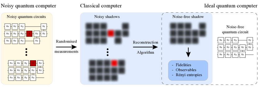
Figure 1: In the present work we assume we only have access to a noisy quantum computer (left) such that every circuit we run (left, yellow area) gets corrupted by gate noise (unwanted red gate elements). We aim to extract properties of a state that would be prepared by an ideal quantum computer (right) with the use of powerful error mitigation techniques. We provide a rigorous theoretical framework for PEC shadows which effectively allows us to obtain a classical shadow of the ideal quantum state (noise-free shadow) from which we can predict many ideal properties in classical post-processing (middle blue area, classical computer). In our formalism we run a series of distinct quantum circuit variants (left, yellow area) that cast different classical shadows (noisy shadows) due to gate noise and due to our intentional recovery operations (red gate elements and their shadows). Under the assumption that the device’s error characteristics have been appropriately learned, we can estimate the noise free shadow (middle) via classical post-processing.

Another major challenge is that near-term quantum algorithms typically require an extreme number of circuit repetitions in order to suppress shot noise [17, 18, 19, 20]. Classical shadows were introduced relatively recently [21] and represent another promising angle in achieving practical quantum advantage. The approach allows one to extract many properties of a quantum state without having to repeat the measurement many times. This is achieved by performing measurements in randomized bases. The measurement outcomes as bitstrings, along with the indexes of the measurement bases form a classical shadow which is an efficient classical representation of the entire quantum state. Shadows have become an entire subfield and various promising applications have been proposed [22, 23] that greatly benefit from the rich information one can access via shadows. For instance, in shadow spectroscopy [23], we estimate many time-dependent expected values from time-evolved quantum states, which then allows us to reveal accurate spectra through the use of efficient classical post-processing.

The focus of the present work is to amalgamate quantum error mitigation techniques with classical shadows. It is worth noting that prior works have considered fruitful connections between quantum error mitigation and classical shadows. First, ref. [24, 25] use classical shadows obtained from a noisy quantum state to perform purification-based error mitigation [26, 27, 28] offline, with only access to a single copy of the state but at an exponential complexity in the number of qubits. Second, the mitigation of errors in the randomised measurements have similarly been addressed in [29, 30].

In the present work we address a distinct problem: Previous methods have assumed that the task involves extracting information from a predetermined quantum state $\rho$, such as the output of a quantum device. However, we consider the practically more relevant scenario where the state $\rho$ is generated by a noisy quantum circuit, and our aim is to mitigate the impact of errors induced by the noisy quantum gates. Our focus is thus to extract properties of an ideal state $\rho_{id}$, which would be generated by a noise-free quantum computer. This approach is a generalisation of quantum error mitigation techniques which generally aim to extract an ideal expected value $\mathrm{Tr}[O\rho_{id}]$ when only noisy measurements $\mathrm{Tr}[O\rho]$ are available. In contrast, the techniques we present are not restricted to a single expected value but instead provide efficient classical representations of the ideal quantum state $\rho_{id}$ through powerful classical shadows as illustrated in Fig. 1.

While we cover most classes of conventional error mitigation techniques, such as Probabilistic Error Cancellation (PEC), Zero Noise Extrapolation (ZNE) and Symmetry Verification (SV), we find that PEC is the most amiable to be used in combination with classical shadows. We thus dedicate most attention to PEC shadows for which we establish a comprehensive theory: Assuming the error model of the quantum gates has been appropriately learned, we rigorously prove that our PEC shadow is an unbiased estimator of the ideal quantum state $\rho_{id}$. We also furnish explicit, efficient classical reconstruction algorithms that enable the simultaneous prediction of linear and non-linear properties of $\rho_{id}$.

Similarly to conventional error mitigation techniques, the ability of estimating properties of the noise-free scenario comes at the cost of an increased statistical variance which implies an increased number of circuit repetitions. We establish rigorous bounds on sample complexities and our results indicate that: (a) the sample complexity of PEC shadows is identical to that of conventional shadows up to a multiplicative factor, and (b) this multiplicative factor $\lVert g\rVert_{1}$ has already been known in the literature as the sample overhead of the PEC approach [13]. Thus the present techniques are efficient in the sense that sample complexities are independent of the number of qubits – but of course the overhead grows exponentially with the number of noisy gates.

In numerical simulations we showcase a broad range of useful practical applications that will play a crucial role in both the near-term and in the early fault-tolerance era. These examples comprise: (a) determining error mitigated energies in variational quantum circuits, which constitutes a fundamental subroutine in near-term applications; (b) predicting many properties simultaneously in ground state preparation to extract two-point correlators or to accelerate the training of circuit parameters[21, 22, 23]; (c) extracting error mitigated local entanglement entropies of a ground state that is prepared by a noisy quantum circuit. Moreover, we discuss several other applications that will significantly benefit from our efficient amalgams of quantum error mitigation and classical shadows.

This paper is organised as follows. In the following section we first briefly review the formalism of classical shadows. Then in Section III we introduce our main result as Probabilistic Error Cancelled shadows. In Section IV we discuss how to combine further error mitigation techniques with classical shadows but conclude that PEC shadows admit the most natural formalism. Finally, in Section V we demonstrate powerful applications of our approach and then conclude in Section VI.

II Preliminaries: classical shadows

The original idea of classical shadow tomography is to apply to the quantum system of $N$ qubits prepared in a specific state $\rho$ a unitary $Q_{j}$ randomly sampled from a certain ensemble $\mathcal{Q}$; typically the ensemble corresponds to just rotating the individual qubits with single-qubit unitaries (Pauli basis measurements) or applying Clifford rotations. This is followed by a measurement in the computational basis, yielding a bitstring $b\in\{0,1\}^{N}$ as the outcome; This bitstring is logged along with the measurement basis forming the index $l=(j,b)$. The collection of these indexes from many independent runs of the protocol then allow us to construct a classical shadow of the state. A classical shadow provides a description of the quantum state that can be classically efficiently stored and manipulated, bypassing the computationally-expensive reconstruction of the full density matrix [21].

II.1 Classical shadows via idealised measurements

We mathematically describe a particular measurement outcome $l=(j,b)$ by the positive operator as $E_{l}{=}p_{j}Q_{j}^{\dagger}|b\rangle\langle b|Q_{j}$; The probability $q_{l}=\mathrm{Tr}(\rho E_{l})$ of this outcome is a product of a (classical) probability $p_{j}$ of choosing a unitary $Q_{j}$ and the probability of observing the bitstring $b$ given the rotated measurement basis. The shadow protocol can be therefore compactly described by a set $E$ of $N_{E}=2^{N}|\mathcal{Q}|$ positive operators given by

$$E=\{E_{l}{=}p_{j}Q_{j}^{\dagger}|b\rangle\langle b|Q_{j},\,\text{with}\,Q_{j}\in\mathcal{Q},\,b\in\{0,1\}^{N}\}.$$ (1)

In the literature, such a collection $E$ of positive operators $E_{l}$ that sums up to the identity is referred to as a generalised measurement (positive operator-valued measure - POVM) and $E_{l}$ are called its effects [31]. It has been shown that formulating shadow tomography using POVMs brings various advantages [32]. Particularly relevant to our purpose, this formulation allows one to automatically account for errors in measurements, which include both read-out errors and gate errors in the implementation of the random unitaries $Q_{j}$ [12, 33, 34, 30, 29]. This is carried out by simply adjusting the effects $E_{l}$ appropriately [32, 35] as we detail towards the end of this section.

Given the above generalised measurement, a single outcome $l=(j,b)$ can be used to construct a snapshot as $\hat{\rho}_{l}=C_{E}^{-1}(E_{l})$ where the channel $C_{E}$ is defined by

$$C_{E}(\rho)=\sum_{l=1}^{N_{E}}\mathrm{Tr}[\rho E_{l}]E_{l},$$ (2)

which is invertible if $E$ spans the whole space of observables [21, 32]. The snapshot can be thought of as single-shot-estimator of the prepared state $\rho$. In an experiment one repeats the above single-shot procedure $N_{s}$ times, which produces a collection of outcomes $\{l_{1},l_{2},\ldots,l_{N_{s}}\}$. Accordingly, a collection of snapshots can be constructed

$$S(\rho,N_{s})=\{\hat{\rho}_{l_{1}},\hat{\rho}_{l_{2}},\dots\hat{\rho}_{l_{N_{s}}}\},$$

which is called a classical shadow of $\rho$. The classical shadow allows us to obtain an unbiased estimate for the density operator in the sense $\rho=\mathbb{E}_{l}[\hat{\rho}_{l}]$.

Crucial to the advantage of shadow tomography is that when the measurement $E$ consists of independent measurements on individual qubits, the snapshots $\hat{\rho}_{l}$ also factorise into a tensor product over the qubits. It is therefore sufficient to store single-qubit tensoring factors of $\hat{\rho}_{l}$, instead of the exponentially large matrix itself [21]. Functions of the density operator with appropriate locality, such as correlation functions or the Rényi entropy, can also be efficiently estimated [21]. As an example, for experimentally-friendly case of randomised noiseless Pauli basis measurements on the qubits, the snapshot corresponding to $l=(j,b)$ is given explicitly by

$$\hat{\rho}_{l}=\bigotimes_{i=1}^{N}\Big{[}3(Q^{(i)}_{j})^{\dagger}|b^{(i)}\rangle\langle b^{(i)}|Q^{(i)}_{j}-\openone\Big{]}.$$ (3)

Above $b^{(i)}$ is the $i^{th}$ bit of the $N$-qubit measurement outcome bitsring $b$, and $Q^{(i)}_{j}$ is the $i^{th}$ single-qubit basis transformation in the applied $N$-qubit Pauli basis transformation $Q_{j}$. In the following, we focus on this practically-pivotal randomised Pauli-measurement scheme. However, our general formalism can immediately be applied to other unitary ensembles such as matchgates [36], Clifford circuits [21] and beyond [37].

II.2 Mitigating readout errors

An advantage of having introduced classical shadows through generalised measurements (POVMs) is that it is now straightforward to incorporate readout-error mitigation techniques [32]. In particular, readout errors refer to the classical process of incorrectly assigning the labels $b$ to the measurement outcome. While in ion-trap devices readout errors may not be significant, i.e., below error levels of gate operations [38, 39], in solid-state devices these errors can be quite substantial and can be on the order of several percent [40]. We illustrate the approach by considering a simple readout-error model where entries in the bitstring $b$ undergo random and independent bit flips ($i^{th}$ bit is flipped as $0\rightarrow 1$ with probability $\alpha_{i}^{+}$ and as $1\rightarrow 0$ with probability $\alpha_{i}^{-}$) – while existing techniques for addressing correlated readout errors as well as gate errors in the shadow basis rotations are indeed similarly applicable [41, 33, 13, 32]. As a consequence, the idealised measurement operators $\outerproduct{0}{0}$ and $\outerproduct{1}{1}$ on the $i^{th}$ qubit are replaced according to the readout error model, in the present case by $(1-\alpha_{i}^{+})\outerproduct{0}{0}+\alpha_{i}^{-}\outerproduct{1}{1}$ and by $\alpha_{i}^{+}\outerproduct{0}{0}+(1-\alpha_{i}^{-})\outerproduct{1}{1}$, which then allows us to explicitly build the effects in Eq. 1 and invert the measurement channels in Eq. 2.

For example, we can analytically obtain a simple formula for the Pauli measurement snapshot from Eq. 3 for the specific readout-error model when $\alpha_{i}^{+}=\alpha_{i}^{-}=:\alpha_{i}$ as

$$\hat{\rho}_{l}=\bigotimes_{i=1}^{N}\Big{[}\frac{3}{1-2\alpha_{i}}(Q^{(i)}_{j})^{\dagger}|b^{(i)}\rangle\langle b^{(i)}|Q^{(i)}_{j}-\frac{1+\alpha_{i}}{(1-2\alpha_{i})}\openone\Big{]}.$$

In the more realistic case when $\alpha_{i}^{+}\neq\alpha_{i}^{-}$ the snapshots can still be computed straightforwardly by numerically (rather than analytically) inverting the single-qubit channel in Eq. 2, model-free readout-error mitigation is also applicable [42]. In conclusion, as measurement-error mitigation techniques are completely decoupled from mitigating state-preparation errors, our mathematical theorems will quantify the sample complexity of the latter, while we demonstrate in numerical simulations that it is indeed straightforward to combine measurement-error mitigation techniques with the present approach.

III Probabilistic error cancelled shadows

While PEC has been used in the literature to remove the bias in expected-value measurements [13], here we apply it to classical shadows to obtain an efficient, classical representation of the entire ideal, noise free state $\rho_{id}$. While this procedure even allows us to estimate the full density matrix $\rho_{id}$, we will focus on efficient practical applications such as simultaneously predicting many properties of $\rho_{id}$. At a technical level PEC shadows is a combination of two random processes, i.e., sampling circuit variants $\mathcal{G}_{\underline{k}}$ and sampling the bitstrings and the basis transformations that form a shadow.

III.1 Probabilistic error cancellation

PEC is one of the most broadly studied error mitigation techniques [43, 44, 13] and indeed has been implemented experimentally [13, 14, 15, 16]; It is performed by decomposing the channel $\mathcal{U}$ of an ideal unitary gate into a linear combination of noisy physical gate operations $\mathcal{G}_{k}$ as $\mathcal{U}=\sum_{k}\gamma_{k}\mathcal{G}_{k}$. Negative quasiprobabilities $\gamma_{k}<0$ are required to formally implement the inverse of a noise channel. Thus the above operation is nonphysical, similarly as the inverse measurement channels of the shadow protocols are nonphysical operations. For this reason, PEC only applies the decomposition in classical post-processing, at the level of expected values and allows us to compute ideal expected values as a linear combination of noisy ones as $\sum_{k}\gamma_{k}\mathrm{Tr}[O\mathcal{G}_{k}|0\rangle\langle 0|]$.

Let us first give an overview of efficient methods that have been developed to accurately identify the coefficients $\{\gamma_{k}\}$ for the quasi-probability decomposition [45, 46, 47, 48, 13]. The simplest such approach exploits that noise models are approximately local and one can thus efficiently characterise the local noise channel of each gate and invert them classically. Recent advances allow for non-local noise models of the form $\Lambda^{G}=e^{\mathcal{L}}$ to be efficiently learned for the case of sparse Pauli operations $\mathcal{L}$ resulting in a trivial inverse of the channel as $\Lambda^{G-1}$ [47]. Making the assumption that $\mathcal{U}$ is supported only on the space spanned by the noisy operations $\mathcal{G}_{k}$, one then randomly applies circuit variants that implement the operations $\mathcal{G}_{k}$ in the inverse noise channel. Under this assumption, theoretical guarantees have been derived on the sample complexity of learning the error model [47]. Given the noise model can be learned prior to the experiment with a constant overhead, we assume in this work that a sufficiently high-precision estimate is available 

Indeed a considerable experimental challenge is posed by the possible drift of the error models over time which may necessitate the repetition of the learning procedure every so often further increasing its sample budget. Let us finally note that our scope goes beyond mitigation of physical gate errors and the formalism developed here can be immediately applied to other scenarios, such as the following. a) Overcoming finite rotation-angle resolution whereby the quasiprobability decomposition is known exactly [50] b) Mitigating logical errors in early-fault tolerant devices whereby the dominant source of noise may arise from imperfect magic-state distillation but noise characterisation and mitigation are effectively identical to the presently considered formalism [51, 52, 53].

We consider that an ideal quantum state $\rho_{id}:=\mathcal{U}_{circ}|0\rangle\langle 0|$ is prepared by an ideal circuit of $\nu$ gates whose channel we denote as $\mathcal{U}_{circ}=\mathcal{U}_{\nu}\cdots\circ\mathcal{U}_{2}\circ\mathcal{U}_{1}$. By introducing the vector notation $\underline{k}=(k_{1},k_{2},\dots k_{\nu})$, we can compactly represent the decomposition of this circuit into noisy gate sequences as $\mathcal{U}_{circ}=\sum_{\underline{k}}g_{\underline{k}}\mathcal{G}_{\underline{k}}$. Here the index $\underline{k}$ indexes all possible gate sequences as

$$\mathcal{G}_{\underline{k}}=\mathcal{G}^{(1)}_{k_{1}}\mathcal{G}^{(2)}_{k_{2}}\cdots\mathcal{G}^{(\nu)}_{k_{\nu}},\quad\quad g_{\underline{k}}=\gamma^{(1)}_{k_{1}}\gamma^{(2)}_{k_{2}}\cdots\gamma^{(\nu)}_{k_{\nu}},$$ (4)

and as shown above the corresponding quasiprobabilities $g_{\underline{k}}$ factorise (the superscript indexes individual gates, e.g., $\mathcal{G}^{(1)}_{k_{1}}$ stands for the decompositon of $\mathcal{U}_{1}$). We now define the quasiprobability decomposition of a quantum circuit.

Definition 1.

We define the quasiprobability decomposition of an ideal circuit $\mathcal{U}_{circ}$ via the set $G:=\{(g_{\underline{k}},\mathcal{G}_{\underline{k}})\}_{\underline{k}}$. We also define the associated probability distribution $p(\underline{k}):=|g_{\underline{k}}|/\lVert g\lVert_{1}$ and here the norm factorizes as $\lVert g\lVert_{1}=\prod_{k=1}^{\nu}\lVert\gamma^{(k)}\rVert_{1}$ into a product of individual norms.

The above quasiprobability decomposition has been used for estimating the ideal expected value of an observable $O$, $\mathrm{Tr}[O\mathcal{U}_{circ}|0\rangle\langle 0|]$, by randomly sampling the noisy expected values $\text{sign}(g_{\underline{k}})\mathrm{Tr}[O\mathcal{G}_{\underline{k}}|0\rangle\langle 0|]$ according to the probability distribution $p(\underline{k})$ and linearly combining them in a classical post-processing step [43, 44, 13]. The norm $\lVert\gamma^{(k)}\rVert_{1}$ can be evaluated straightforwardly for any probabilistic error model: Assuming that during the execution of the $k^{th}$ gate an error happens with probability $p_{k}$, e.g., Pauli errors, we obtain the single-gate norm $\lVert\gamma^{(k)}\rVert_{1}=(1+p_{k})/(1-p_{k})$ [13]. Thus, the cost of error mitigation—as the product of these individual norms from Definition 1—grows as $\lVert g\lVert_{1}\in O(e^{2\xi})$ with the expected number $\xi=\sum_{k}p_{k}$ of errors in the full circuit, rendering the approach impractical when $\xi\gg 1$ [43, 44, 13].

III.2 Details of the protocol

We start by applying the PEC protocol in a more general setting such that the quasiprobability decomposition allows us to obtain an unbiased estimator of the full density matrix.

Lemma 1.

Given a quasiprobability decomposition $G$ from Definition 1, by sampling the noisy circuits $\mathcal{G}_{\underline{k}}$ according to the probability distribution $p(\underline{k})$ we obtain an unbiased estimator of the ideal density matrix $\rho_{id}:=\mathcal{U}_{circ}|0\rangle\langle 0|$ as

$$\hat{\rho}_{id}=\lVert g\lVert_{1}\,\mathrm{sign}(g_{\underline{k}})\mathcal{G}_{\underline{k}}|0\rangle\langle 0|$$ (5)

in the sense that $\mathbb{E}_{\underline{k}}[\hat{\rho}_{id}]=\rho_{id}$.

The above estimator has a clear operational meaning: (1) choose a multi-index $\underline{k}$ randomly according to the probability distribution $p(\underline{k})$ and run the noisy quantum circuit $\mathcal{G}_{\underline{k}}$; (2) the output state $\mathcal{G}_{\underline{k}}|0\rangle\langle 0|$ is a density matrix that we multiply by $\mathrm{sign}(g_{\underline{k}})$ and with the norm $\lVert g\lVert_{1}$; (3) formally, the mean of these matrices is an estimate of the ideal density matrix $\rho_{id}$.

Regrettably, the above protocol is purely formal as the multiplication with negative quasiprobabilities is non physical and could only be achieved in post-processing, e.g., after fully reconstructing the density matrix. We thus exploit classical shadows as a powerful tool for obtaining an efficient classical description of the states which can then be naturally assigned negative quasiprobabilities in classical post-processing. Indeed, snapshots are not physical density matrices either, as is apparent in Eq. 3. We now state our protocol that serves as an unbiased estimator of the ideal state.

Theorem 1 (PEC shadows).

Given a quasiprobability decomposition $G$ of the ideal circuit $\mathcal{U}_{\text{circ}}$ from Definition 1, and a classical shadow protocol with the POVM measurement $E$ from Eq. 1, we define PEC shadows as the set $H:=\{(g_{\underline{k}},\mathcal{G}_{\underline{k}},E_{l})\}_{\underline{k},l}$ and define the corresponding PEC snapshot as

$$\hat{\rho}_{id}:=\hat{\rho}_{\underline{k},l}=\lVert g\rVert_{1}\,\mathrm{sign}(g_{\underline{k}})C_{E}^{-1}(E_{l}).$$ (6)

We will often use the notation $\hat{\rho}_{id}$ to abbreviate $\hat{\rho}_{\underline{k},l}$ as it is an unbiased estimator of the ideal density matrix $\rho_{id}$ such that $\mathbb{E}[\hat{\rho}_{id}]=\underset{\underline{k},l}{\mathbb{E}}[\hat{\rho}_{\underline{k},l}]=\rho_{id}$.

Above the averaging $\mathbb{E}[\cdot]$ happens not only over the effects $E_{l}$ indexed by $l$ (all basis transformations and all measurement outcomes), but additionally we average over all circuit variants indexed by $\underline{k}$. The reason is that the measurement $E=\{E_{l}\}_{l}$ is not performed on a fixed input density matrix $\rho$ as in conventional shadows but rather on the quasiprobability decomposition of the ideal state $\rho_{id}\propto\mathcal{G}_{\underline{k}}|0\rangle\langle 0|$. Let us now summarise the resulting experimental protocol.

• choose randomly a multi-index $\underline{k}$ according to the probabilities $p(\underline{k})$ and store the $\text{sign}(g_{\underline{k}})$

• choose uniformly randomly a unitary rotation $Q_{j}\in\mathcal{Q}$ and store its index $j$

• execute in a quantum computer the gate sequence $\mathcal{G}_{\underline{k}}$, the unitary rotation $Q_{j}$, perform a measurement in the standard basis and finally register its outcome $b$

• each stored index $(\text{sign}[g_{\underline{k}}],j,b)$ uniquely identifies a classical snapshot $\hat{\rho}_{\underline{k},l}=\lVert g\rVert_{1}\,\mathrm{sign}(g_{\underline{k}})C_{E}^{-1}(E_{l})$ where recall that $E_{l}$ is a POVM effect with the index $l=(j,b)$ from Eq. 1

• repeat the procedure and collect $N_{s}$ classical snapshots to build a classical shadow of the ideal state $S(\rho_{id},N_{s})=\{(\hat{\rho}_{id})_{1},(\hat{\rho}_{id})_{2},\dots,(\hat{\rho}_{id})_{N_{s}}\}$

The classical dataset $S(\rho_{id},N_{s})$ can then be classically post-processed offline and we detail explicit algorithms for predicting local properties in Section III.4.

Note that PEC shadows produce a distribution of snapshots that is different than directly applying conventional shadows to a noise-free state $\rho_{id}$, albeit with an identical mean. The reason is that each circuit variant $\mathcal{G}_{\underline{k}}$ in Eq. 5 yields a different distribution of classical snapshots. For example, in the next section we prove bounds on variances of PEC shadows and find that they are indeed increased compared to conventional shadows applied directly to $\rho_{id}$.

III.3 Rigorous performance guarantees

We first consider the pivotal practical application as predicting error mitigated expected values of observables $O$ via the estimator $\hat{o}=\mathrm{Tr}[O\hat{\rho}_{id}]$. A key observation is that in error mitigation techniques the ability to predict noise-free expected values comes at the cost of an increased statistical variance which implies an increased number of circuit repetitions. We now bound the variance of any operator’s expected value.

Lemma 2 (variance of linear properties).

Given an observable $O$ and the PEC snapshot $\hat{\rho}_{id}$ from Theorem 1, the variance of $\hat{o}=\mathrm{Tr}[O\hat{\rho}_{id}]$ can be upper bounded as

$$\mathrm{Var}[\hat{o}]\leq\lVert g\rVert_{1}^{2}\,\lVert O\rVert_{E}^{2},$$ (7)

where $\lVert\cdot\rVert_{E}^{2}$ is the shadow norm of the observable $O$ as defined in Lemma 3. When $O$ is a $q$-local Pauli string and we use Pauli basis measurements then $\lVert O\rVert_{E}^{2}=3^{q}$ as we detail in Lemma 3.

We explain in Appendix D that we can account for the cost of readout-error mitigation via the above shadow norm, which becomes $3^{q}(1{-}2\alpha)^{-2q}$ when considering a simple readout-error model with probability at most $\alpha$. Observe that the above variance depends on two factors: The first one is the squared shadow norm $\lVert O\rVert_{E}^{2}$ which determines the sample complexity of conventional shadows [21]; The second factor is a multiplicative term $\lVert g\rVert_{1}^{2}$ which accounts for the well-known measurement overhead associated with the conventional PEC protocol [43, 44, 13]

We defer further discussion to Section A.2 where we also explain how the shadow norm depends on the unitary ensemble $\mathcal{Q}$: While we only state explicitly the shadow norm for the practically most important ensemble of Pauli basis measurements, we note that bounds for other ensembles are immediately available in the literature [36, 21, 37]. Furthermore, we also explain in Section B.1 that the above bound is expected to be pessimistic due to an even more significantly overestimated constant prefactor than in conventional shadows.

Following the approach of [21] we use concentration properties of the median of means estimator to derive rigorous sample complexities: for the simultaneous prediction of many observables $O_{1},\dots,O_{M}$ we exponentially suppress statistical outliers by splitting the PEC shadows $S(\rho_{id},N_{s})$ into independent batches and then computing a median of the means as we detail in Section B.2. The resulting bounds depend on two performance metrics as the accuracy $\epsilon$ and the success probability $\delta$.

Theorem 2 (informal summary).

Given the PEC shadows $H:=\{(g_{\underline{k}},\mathcal{G}_{\underline{k}},E_{l})\}_{\underline{k},l}$ from Theorem 1 we want to simultaneously estimate expected values of $M$ operators in the ideal state as $\mathrm{Tr}[O_{1}\rho_{id}]\dots\mathrm{Tr}[O_{M}\rho_{id}]$. Using a median of means estimator, the number of shots required to achieve performance parameters $\epsilon,\delta\in[0,1]$ is

$${}N_{s}=32\epsilon^{-2}\,\,\log(\frac{M}{\delta})\,\,\lVert g\rVert_{1}^{2}\,\,\max_{1\leq k\leq M}{\lVert O_{k}\rVert_{E}^{2}},$$ (8)

where we use the largest shadow norm $\lVert O_{k}\rVert_{E}^{2}$. Refer to Theorem 4 for a formal statement of this theorem.

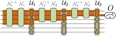
Figure 2: Illustration of the light cone of an observable $O$ which is represented by the measurement apparatus and only acts nontrivially on the second (from top) qubit. The orange area indicates the qubits which are contained in the light cone $\mathcal{I}$ of the observable with respect to the ideal quantum circuit (orange boxes) $\mathcal{U}_{3}\mathcal{U}_{2}\mathcal{U}_{1}$. To simplify derivations we assume the gate noise channels $\mathcal{N}_{k}$ are local (light green boxes) such that they are contained within the lightcone $\mathcal{I}$ but our results can be extended to non-local models via [54].

Finally, we consider predicting non-linear properties of the state of the form $\mathrm{Tr}[O(\rho_{id})^{m}]$. Following ref. [21] we use the fact that a polynomial function in the quantum state can be written as a linear function in tensor products of the state, for example, $\mathrm{Tr}[O(\rho_{id})^{2}]=\mathrm{Tr}[\tilde{O}\rho_{id}\otimes\rho_{id}]$ with $\tilde{O}=\mathrm{SWAP}(O\otimes\openone)$ where the SWAP operator swaps the two copies. In Section B.3 we detail our construction using U-statistics to derive unbiased estimators in terms of the classical snapshots, e.g., for $m=2$ we select all distinct pairs of snapshots $(\hat{\rho}_{id})_{i}\otimes(\hat{\rho}_{id})_{j}$ with $i\neq j$. We can bound the variance of any non-linear property as follows.

Theorem 3 (variance of nonlinear properties).

Given our PEC snapshots $\hat{\rho}_{id}$ from Theorem 1 we can estimate polynomial properties of degree $m$ of the ideal state $\rho_{id}$ via U-statistics of tensor products of all distinct snapshots. The number of samples required to predict the non-linear property scales as $N_{s}\in\mathcal{O}(||g||_{1}^{2m}/\epsilon^{2})$ for a desired accuracy $\epsilon$. Refer to Section B.3 for details.

One can similarly apply a median of means estimator to enable simultaneous prediction of many non-linear properties: We detail an explicit protocol in the next section for simultaneously estimating many local Rényi entropies. Note that measurement overhead $||g||_{1}^{2m}$ grows with the $2m^{th}$ power of the quasiprobability norm consistent with our effective construction of $m$ copies of the original noisy circuit which leads to an effective $m$-fold increase in the number of noisy gates.

III.4 Classical post-processing algorithms

In this section we summarise reconstruction algorithms for the practically pivotal scenario of Pauli basis measurements from Section II.

Algorithm 1 (local Pauli strings).

The expected value of a $q$-local Pauli observable $P$ in a PEC snapshot can be calculated analytically as

$$\mathrm{Tr}[P\hat{\rho}_{\underline{k},l}]=\lVert g\rVert_{1}\,3^{q}\,\text{sign}(g_{\underline{k}})f(b,Q_{j}).$$

The reconstruction algorithm iterates over all snapshots in the shadow $S(\rho_{id},N_{s})$ and calculates the median of means of the above expression using a number of batches provided by the user. Here $f(b,Q_{j})\in\{\pm 1,0\}$ results in $0$ if the measurement bases in $Q_{j}$ are incompatible with $P$ and $\pm 1$ if the measurement bases are compatible with $P$ while the sign is determined by the bitstring $b$. The algorithm has runtime $\mathcal{O}(qN_{s})$. ∎

We defer the detailed derivation to Section C.1. Note that the above error mitigated reconstruction algorithm deviates from that of [21] as the individual snapshot outcomes are multipiled with the norm $\lVert g\rVert_{1}$ and signs of the quasiprobabilities $\mathrm{sign}(g_{\underline{k}})$.

Since we reconstruct $q$-local Pauli observables, we can significantly reduce the sample variacne via light-cone arguments [55, 54]. In Fig. 2 we illustrate the light cone that an observable creates with respect to the ideal unitary circuit $\mathcal{U}_{circ}$. To simplify the following arguments we assume local noise models to guarantee the same light cone is valid for all gate sequences $\mathcal{G}_{\underline{k}}$, however, it is straightforward to extend the arguments to non-local noise following [54].

We observe that for each gate that is not within the light cone of the observable $P$ we can “turn off” PEC thereby not wasting our measurement budget on mitigating noisy gates that do not affect our observable.

Algorithm 2 (light cones).

Given a $q$-local Pauli string $P$ we define the set of indexes of all gates in the light cone of the obserable as $\mathcal{I}:=\{l\,|\,\mathcal{U}_{l}\,\text{is in the light cone of $P$}\}$. We then simply use Algorithm 1 with a modified set of quasiprobabilities from Definition 1 as

$$\lVert\tilde{g}\rVert_{1}=\prod_{l\in\mathcal{I}}\lVert\gamma^{(l)}\rVert_{1},\quad\text{and}\quad\text{sign}(\tilde{g}_{\underline{k}})=\prod_{l\in\mathcal{I}}\text{sign}\gamma^{(l)}_{k_{l}}.$$

The algorithm has the same asymptotic runtime $\mathcal{O}(qN_{s})$ as Algorithm 1 and only incurs a negligible preprocessing time to determine the index set $\mathcal{I}$ specifically for each $P$. ∎

Refer to Section C.2 for a derivation. The measurement cost $\lVert\tilde{g}\rVert_{1}$ is thus determined by the number of gates in the light cone of $P$ rather than by the total number of gates $\nu$. Imagine, for example, noisy quantum gates with $\lVert\gamma^{(l)}\rVert_{1}=1{+}p$; the measurement cost is determined by $(1{+}p)^{|\mathcal{I}|}$ as opposed to the worst case $\lVert\tilde{g}\rVert_{1}=(1{+}p)^{\nu}$ where $\nu$ is the total number of noisy gates as detailed in Ref. [54]. A significant advantage of this procedure is that it does not require one to modify the experimental protocol, i.e., the noise in all gates can be mitigated in the shadows.

Finally, we consider estimating Rényi entropies via the purities $\mathrm{Tr}\left(\rho_{Q}^{2}\right)$ as $R_{Q}:=-\log\mathrm{Tr}\left(\rho_{Q}^{2}\right)$ where $\rho_{Q}$ is the reduced density matrix of the subsystem $Q$.

Algorithm 3 (local purities).

Given a subsystem as the set of qubits $Q=\left\{q_{1},...,q_{m}\right\}$, an unbiased estimator for the respective purity is obtained as

$$\mathrm{Tr}\left(\hat{\rho}_{Q}^{2}\right)=\lVert g\rVert_{1}^{2}\text{sign}(g_{i})\text{sign}(g_{j})f(i,j,Q).$$ (9)

Here $i$ and $j$ abbreviate indexes of the snapshots as, e.g., $i=(\underline{k},l)$ and $i\neq j$. The algorithm iterates over all distinct pairs of snapshots in the shadow $S(\rho_{id},N_{s})$ and calculates the median of means of the above expression. The factors $f(i,j,Q)$ depend only on whether the measurement bases and outcome bitsrings are identical within the subsystem $Q$. The algorithm has a runtime $\mathcal{O}(|Q|N_{s}^{2})$. ∎

We defer the detailed derivation to Section C.1. Note that the runtime is linear in the subsystem size and quadratic in the number of shots. For sufficiently small subsystems and large numbers of shots it might be preferred to use the exponentially $\mathcal{O}(4^{|Q|}N_{s})$ scaling algorithm of [21].

IV Further error mitigation techniques

IV.1 Error extrapolated shadows

The key idea behind zero-noise extrapolation resides in the possibility of increasing the noise in the circuit and extrapolating expected values back to the case of zero noise. The approach is intuitive to use, requires less resources than PEC but yields a biased estimator. A non-trivial aspect, however, is choosing the correct model function for the extrapolation which has been extensively discussed in the literature [13, 44, 14]; typical models include a linear function, an exponential function or a linear combination of multiple exponentials.

We consider extrapolation as a means for mitigating errors in properties extracted from classical shadows. The key ingredient we require is the ability to generate a collection of shadows at different noise strengths $S(\rho_{p_{0}},N_{s}),...,S(\rho_{p_{n}},N_{s})$ such that $p_{k}\geq p_{0}$ and $p_{0}$ is the device’s lowest possible noise strength. These shadows enable us to extract the expected values $f_{m}(p)=\mathrm{Tr}[O_{m}\rho_{p}]$ at a given noise level $p$. By fitting a suitable model function $\tilde{f}_{m}(p)$, e.g., a linear model, to this dataset we can approximate ideal properties of the state using an extrapolation via the limit

$$\mathrm{Tr}[O_{m}\rho_{id}]\approx\lim_{p\rightarrow 0}\tilde{f}_{m}(p).$$

While we could certainly leverage existing techniques for physically increasing noise rates in a circuit to obtain $S(\rho_{p},N_{s})$ [14, 13], we can also exploit the power and flexibility of the previously derived PEC shadow approach: Instead of considering the quasiprobability representation of the ideal circuit in Definition 1 we can rather decompose the noise-boosted circuits as $\mathcal{G}_{circ}(p)=\sum_{\underline{k}}g_{\underline{k}}(p)\mathcal{G}_{\underline{k}}$ with non-negative probabilities $g_{\underline{k}}(p)$. For example, in the case of local depolarising noise the circuit variants $\mathcal{G}_{\underline{k}}$ are simply obtained by randomly inserting Pauli $X$, $Y$ or $Z$ operations after each noisy gate with probabilities $p{-}p_{0}$. Furthermore, Lindblad-Pauli learning directly gives access to the continuous set of circuits $\mathcal{G}_{circ}(p)$ [47].

Let us now state a corollary to Theorem 1 that allows us to obtain the shadows of error boosted states $\rho_{p}:=\mathcal{G}_{circ}(p)\rho_{ref}$.

Corollary 1 (error-boosted shadows).

We consider the parametric quasiprobability decomposition $G$ as noise-boosted circuits $\mathcal{G}_{circ}(p)$ with $p\geq p_{0}$. The PEC shadows $H:=\{(g_{\underline{k}}(p),\mathcal{G}_{\underline{k}},E_{l})\}_{\underline{k},l}$ from Theorem 1 result in the simplified snapshots as $\hat{\rho}_{p}:=\hat{\rho}_{p,(\underline{k},l)}=C_{E}^{-1}(E_{l})$ due to $\text{sign}(g_{\underline{k}}(p))=+1$ and $\lVert g(p)\rVert_{1}=1$. It follows that $\hat{\rho}_{p}$ is an unbiased estimator of the noise-boosted density matrix $\rho_{p}$ such that $\mathbb{E}[\hat{\rho}_{p}]=\underset{\underline{k},l}{\mathbb{E}}[\hat{\rho}_{p,(\underline{k},l)}]=\rho_{p}$.

A significant advantage in boosting noise via $p\geq p_{0}$ rather than reducing it is that now every quasiprobability is non-negative $g_{\underline{k}}(p)\geq 0$ and thus we do not incur a measurement overhead in Theorem 2 via $\lVert g(p)\rVert_{1}=1$. Nevertheless, the extrapolated value indeed suffers from an increased variance which implies an increased number of samples and details can be found in the literature [13].

Note that the above scheme can be applied beyond the estimation of expectation values. For instance, one can in principle use shadows to reconstruct partial density matrices $\hat{\rho}_{p}$ at different noise strengths $p$ and apply ZNE to individual matrix entries. However, note that ZNE might require different kinds of model functions $f(p)$ for different properties, e.g., non-linear models for predicting non-linear properties of the state. In contrast, the great advantage of PEC shadows is that it provides an unbiased estimator for the entire quantum state.

IV.2 Symmetry verified shadows

Symmetry verification is another leading quantum error mitigation technique [56, 57]; It exploits that often the ideal states to be prepared $\rho_{id}$ are pure states that obey certain problem specific symmetry group operations described by $S\in\mathbb{S}$. The fact that the ideal state is symmetric then implies that it “lives in” the subspace defined by the projection operator

$$\Pi_{\mathbb{S}}=\frac{1}{|\mathbb{S}|}\sum_{S\in\mathbb{S}}S,$$

which satisfies $\Pi_{\mathbb{S}}^{2}=\Pi_{\mathbb{S}}$.

Given a noisy state $\rho$, one might be able to measure the above symmetries (in fact their generators are sufficient) via, e.g., Hadamard-test circuits, and retain only circuit runs that produce the correct symmetry outcomes [13, 58]. Such post-selection projects the noisy state back into this symmetry subspace producing the effective output state as $\rho_{\textrm{sym}}=\Pi_{\mathbb{S}}\rho\Pi_{\mathbb{S}}/\Tr(\Pi_{\mathbb{S}}\rho)$. We can apply conventional shadow tomography to this symmetry-verified state $\rho_{\textrm{sym}}$ thereby effectively obtaining error mitigated shadows, i.e., an unbiased estimator of $\rho_{\textrm{sym}}$. The sampling overhead of this post-selection technique is $\Tr(\Pi_{\mathbb{S}}\rho)^{-1}$ the inverse of the fraction of circuit runs that pass the symmetry verification process.

Instead of post-selection, we can also perform symmetry verification at the post-processing stage. Suppose we are interested in the expectation value of the ideal state with respect to the target observable $O$, the target expectation value can be written as

$$\Tr(O\rho_{\textrm{sym}})=\frac{\Tr(O\Pi_{\mathbb{S}}\rho\Pi_{\mathbb{S}})}{\Tr(O\Pi_{\mathbb{S}}\rho)}=\frac{1}{|\mathbb{S}|}\frac{\sum_{S,S^{\prime}\in\mathbb{S}}\Tr(SOS^{\prime}\rho)}{\sum_{S\in\mathbb{S}}\Tr(S\rho)}$$

Conventional shadow tomography can be used well in practice for estimating $SOS^{\prime}$ and $S$ for all $S,S^{\prime}\in\mathbb{S}$ when the symmetries are sufficiently local, i.e., they are supported on at most weight-$s$ Pauli operators. Then, given a Pauli observable $O$ of weight at most $q$, the effective observable $SOS^{\prime}$ is then at most of weight-$(2s{+}q)$. However, the sample complexity of conventional shadows with Pauli measurements grows exponentially with the weight of the Pauli string and it is thus crucial that the total weight $2s{+}q$ be reasonably small.

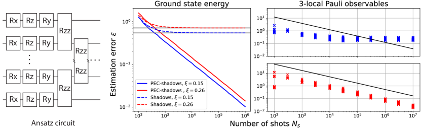
Figure 3: (left) A noisy variational Hamiltonian ansatz is used to prepare the ground state of Eq. 10 but our aim is to learn properties of the noise-free state. (middle) Energy estimation errors for different noise strengths with conventional shadows (dashed blue, dashed red) and with PEC shadows including readout error mitigation (solid blue, solid red). Bias (grey solid lines) is introduced when the ground state energy $\mathrm{Tr}(\rho\mathcal{H})$ is directly estimated from the noisy quantum state $\rho$. Error mitigated shadows are unbiased as they estimate $\mathrm{Tr}(\rho_{id}\mathcal{H})$. Increasing the circuit error rate $\xi$ (blue vs. red) increases the bias in standard shadows (dashed blue vs. dashed red) and increases the variance of the error mitigated shadows (solid blue vs. solid red). Each data point is an average over $10^{4}$ experiments of a fixed shot budget $N_{s}$. (right) Error in simultaneously estimating all 3-local Pauli strings without (blue) and with (red) PEC and readout error mitigation – only the 200 observables of the highest estimation error are shown and a circuit error rate $\xi\approx 0.72$ is assumed. Errors are significantly below our rigorous bounds from Theorem 2 (which also take into account the overhead due to readout errors) for PEC shadows but the errors for conventional shadows can be above their respective bounds from [21] due to bias and readout errors (right end of blue).

For example, a typically used symmetry in fermionic simulation is the fermionic particle number parity which is, however, usually a high-weight operator for standard encodings such as the Jordan-Wigner encoding. Nevertheless, one can use encodings that come with inherent local symmetry generators like Majorana loop encodings [59], or even implement the circuit using some small quantum codes with local stabilisers [60]. However, even if these symmetry generators are local, the number of generators scales with the number of qubits thus some symmetries they generate are still high-weight. Hence, in order to efficiently use shadow techniques, we can apply verification using a constant number of local symmetry generators, such that the highest-weight symmetry that can be generated is upper-bounded by some constant.

We also note that the sampling cost can be reduced when the target observable $O$ commutes with the symmetry projector $\Pi_{\mathbb{S}}$ which is often the case in typical applications. In such a scenario, $\Pi_{\mathbb{S}}O\Pi_{\mathbb{S}}=O\Pi_{\mathbb{S}}$ and thus

$$\Tr(O\rho_{\textrm{sym}})=\frac{\Tr(O\Pi_{\mathbb{S}}\rho)}{\Tr(\Pi_{\mathbb{S}}\rho)}=\frac{\sum_{S\in\mathbb{S}}\Tr(SO\rho)}{\sum_{S\in\mathbb{S}}\Tr(S\rho)}.$$

This way the effective observables we need to estimate from shadows are $SO$ and $S$ for all $S\in\mathbb{S}$ which have a reduced weight $s{+}q$ compared to the previous $2s{+}q$.

V Applications

In this section we showcase how our approach can effectively extend the reach of noisy quantum computers and explore its practical applications. Recall that fully fault-tolerant quantum computers will enable executions of (in principle) arbitrarily deep circuits thus allowing users to extract expected values via, e.g., amplitude estimation, whose time complexity is superior $O(M/\epsilon)$ but is proportional to the circuit depth. In contrast, we focus on application areas where these coherent techniques are prohibitive due to circuit depth limitations, e.g., due to non-negligible logical error rates expected in early fault-tolerant devices. The advantage of classical shadows is that they only require an increase of circuit depth that is independent of the state preparation circuit – and this increase is negligible for Pauli shadows. Since the present approach has a sample complexity $\mathcal{O}(\log(M)/\epsilon^{2})$ it is particularly well suited for applications where the aim is to extract a large number $M$ of properties.

For instance, noisy quantum computers in either the late NISQ era or in the early fault-tolerance era will enable us to simulate the time evolution of quantum states or to prepare ground or eigenstates [17, 18, 19, 22, 23, 61, 62]. Our approach can then be used to accurately and efficiently extract a large number of properties of these states provided that the noise rates are reasonable, i.e., the overhead $\lVert g\rVert_{1}$ is moderate. In these application areas a fixed precision, such as chemical accuracy $\epsilon\approx 10^{-3}$, is often sought [9, 17, 18, 19].

V.1 Ground-state preparation

We first consider a spin-ring Hamiltonian as

$$\mathcal{H}=\sum_{k\in\text{ring}(N)}\omega_{k}Z_{k}+J\vec{\sigma}_{k}\cdot\vec{\sigma}_{k+1},$$ (10)

with coupling $J=0.3$, on-site interaction strengths uniformly randomly generated in the range $-1\leq\omega_{k}\leq 1$ and $\vec{\sigma}_{k}=(\sigma^{x}_{k},\sigma^{y}_{k},\sigma^{z}_{k})^{T}$ is a vector of single-qubit Pauli matrices. This spin problem is relevant in condensed-matter physics in understanding many-body localisation [63] but is challenging to simulate classically for large $N$ [64, 65]. A broad range of techniques are available in the literature for finding eigenstates of such quantum Hamiltonians using near-term or early fault-tolerant quantum computers [17, 18, 19, 22]. Here we prepare the ground state of this model using a variational Hamiltonian ansatz in Fig. 3 (left) of $l=5$ layers on $12$ qubits and, as we detail in Appendix D, we assume a biased Pauli noise model that can be learned efficiently using techniques from [47] while assuming a readout error model from Section II.2.

Ground state energy with PEC: Fig. 3 (middle) shows the error in the ground state energy estimated using conventional shadows (dashed blue and dashed red) and PEC shadows (solid blue and solid red) for an increasing number of shots $N_{s}$.

Our ansatz circuit would ideally prepare the ground state $\rho_{id}$ but due to gate noise we actually prepare the noisy state $\rho$. Thus, conventional shadows (dashed blue, dashed red) converge to a plateau corresponding to the biased energy $\mathrm{Tr}({\rho\mathcal{H}})$ (solid grey). This bias is significantly increased as we increase the circuit error rate from $\xi\approx 0.15$ to $\xi\approx 0.26$ (dashed blue vs. dashed red), which is the expected number $\xi=\sum_{k}p_{k}$ of errors in the full circuit as explained in Section III. In contrast, PEC shadows that include measurement-error mitigation (solid blue and solid red) converge to the true energy $\mathrm{Tr}({\rho_{id}\mathcal{H}})$ in standard shot-noise scaling $O(1/\sqrt{N_{s}})$.

Local properties with PEC: Besides Hamiltonian energy estimation, which is one of the typical subroutines in quantum computing, there is also significant value in simultaneously determining many local observables’ expectation values. For example, the rich information from classical shadows can be used to significantly improve parameter training or to directly estimate Hamiltonian energy gaps through the use of efficient classical post-processing [22, 23]. In Fig. 3(right), we plot errors when simultaneously estimating all 3-local Pauli operators for an increasing number of shots $N_{s}$. Fig. 3(red) shows that the errors in PEC shadows are always significantly below the theoretical bounds (black line) from Theorem 2 confirming looseness of the bounds (assuming success probability $\delta=10^{-3}$, and $M=3^{3}{12\choose 3}=5940$). Fig. 3(blue) shows the errors in conventional shadows are below their bounds (with $\lVert g\rVert_{1}=1$) only for a small number of shots but then asymptotically reach a plateau due to circuit noise.

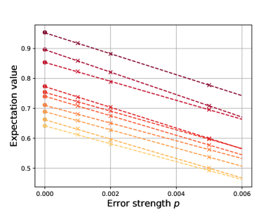
Figure 4: Simultaneously estimating all 3-local Pauli operators using error extrapolated shadows. We estimated noisy expected values (crosses) from shadows of size $N_{s}=10^{7}$ by increasing the native depolarising error rate $p=10^{-3}$ to higher levels $\left\{2\times 10^{-3},5\times 10^{-3}\right\}$ by randomly sampling noisy circuit variants. Using a linear model function we then extrapolate to zero noise to obtain an error mitigated expectation value close to the ideal ones (disks).

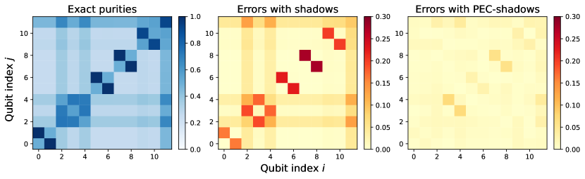
Figure 5: A noisy variational Hamiltonian ansatz is used to prepare the ground state of Eq. 11 whose ideal, noise-free Rényi entropies $R_{Q}$ we can learn with PEC shadows. We plot purities $\mathrm{Tr}(\rho_{Q}^{2})$ as a proxy for $R_{Q}:=-\log\mathrm{Tr}\left(\rho_{Q}^{2}\right)$. (left) Purity heat map in the noiseless case and infinite shot limit. An increasing value indicates that the subsystem $Q$ is less entangled with the remaining qubits. (middle-right) Absolute error in the purities due to gate noise for a circuit error rate $\xi=0.6$ and due to finite repetition using $N_{s}=10^{5}$. (middle) Although the entanglement pattern is approximately recovered with conventional shadows, in some instances we observe substantial errors, i.e., the largest error is $0.27$. (right) Absolute errors with PEC shadows are significantly smaller, i.e., the largest error is $7\times 10^{-2}$ but this figure could be further reduced by increasing $N_{s}$.

Local properties with extrapolation: We now consider the same task of simultaneously estimating expectation values of Pauli operators but we use error extrapolation. Here we start by generating shadows $S(\rho_{p_{1}},N_{s}),...,S(\rho_{p_{n}},N_{s})$ at different noise strengths that we use to compute the noisy Pauli expectation values. Fig. 4 shows 10 examples of expected values (crosses) as a function of noise strength and the respective linear models we fit (dashed lines). The intercept of the fitted model (dashed lines) is our estimate of the exact expected value (disks) and is indeed reasonably close in the example. While ZNE has been very effective and typically has a lower measurement overhead then PEC, it is generally biased.

V.2 Error mitigated estimation of entanglement entropies

Finally, we consider an application for which classical shadows are a primary enabler but for which error mitigation techniques have been less explored [13]. As opposed to studying entanglement properties or verifying the presence thereof in mixed quantum states [66, 67, 68, 69], here our primary goal is to extend the reach of noisy quantum computers: we aim to study entanglement properties of ideally pure states which are prepared by quantum algorithms, such as phase estimation or VQE. For example, near-term quantum computers will enable us to prepare eigenstates [17, 18, 19, 22] of quantum Hamiltonians and error mitigated entanglement measures can be used for, e.g., characterising phase transitions. Similarly, one could simulate the time evolution of a collision of two molecules with an early fault-tolerant quantum computer and investigate how entanglement builds up across the individual subsystems. Furthermore, efficiently characterising many local correlations in a state can be used to train DFT models for accurate classical simulations [70].

We consider the Heisenberg chain

$$\mathcal{H}=\sum_{k}J_{k}\vec{\sigma}_{k}\cdot\vec{\sigma}_{k+1},$$ (11)

with uniformly random $-1\leq J_{k}\leq 1$ and prepare its ground state with a variational Hamiltonian ansatz of $l=8$ layers on $12$ qubits. This system was used in ref. [21] to illustrate the power of classical shadows in predicting entanglement entropies. However, the ground state was approximated by a set of noise-free singlet states [71, 72] whereas we assume a noisy quantum computer is used for state preparation.

We use PEC shadows to extract purities $\mathrm{Tr}(\rho_{Q}^{2})$ for all single and two-qubit subsystems $Q$; These purities then define Rényi entropies as $R_{Q}:=-\log\mathrm{Tr}(\rho_{Q}^{2})$. In Fig. 5, we plot the exact purities in the noiseless case – disjoint blocks involving two qubits confirm that the ground state could be approximated by a tensor product of noise-free singlet states.

Fig. 5 (middle) shows the errors in estimating local purities using shadows of size $N_{s}=10^{5}$ for a circuit error rate $\xi=0.6$. Even for this moderate error rate conventional shadows are significantly impacted by imperfections and result in errors as large as $0.27$ – whereas for an increasing noise rate all purities converge to a constant value of $1/d$ where $d$ is the subsystem dimension. In contrast, PEC shadows drastically improve the accuracy in Fig. 5 (right) and the largest error is approximately $7\times 10^{-2}$ at a number of samples $N_{s}=10^{5}$.

V.3 Further applications

The techniques presented in this work enable us to approximate an unbiased estimator of an ideal noise free state $\rho_{id}$ which can be enabling for a broad range of further practical applications that we defer to follow up works. For example, ref. [21] proposed that classical shadows with randomised Clifford measurements can be used to predict fidelities, such as the fidelity of $\rho$ with respect to a known state $\psi$. One can imagine applications where the fidelity $\langle\psi|\rho|\psi\rangle$ is not a relevant indicator due to the impact of noise on $\rho$ and one rather aims to predict $\langle\psi|\rho_{id}|\psi\rangle$, e.g., to quantify how well a variational quantum circuit or phase estimation can prepare a known ground state thereby verifying a circuit structure under the presence of gate noise.

Furthermore, the quantum Fisher information (QFI), which is a key quantity in quantum metrology, can be bounded and approximated using classical shadows via techniques of Ref. [73]. Indeed, in certain applications the relevant quantity might not be the QFI of the noisy state $\rho$ but rather the QFI of the noise-free state $\rho_{id}$ which can be approximated with our techniques [74].

We also finally note possible “reverse” applications where classical shadows can be used to improve error mitigation techniques; an obvious one is perhaps the use of shadow tomography in explicitly reconstructing the noisy gate channels from Section III – typically one assumes the gate channels are local and thus the approach is efficient. In contrast, in learning-based error mitigation one does not reconstruct the noisy gate channels but rather aims to directly learn the quasiprobabilities $g_{\underline{k}}$ by running classically simulable circuits on a noisy quantum computer and comparing observable expectation values to classically simulated ones [45, 46, 48, 13]. While one can exclusively train a model for one specific observable with conventional measurement schemes, classical shadows allow for simultaneously estimating a large number of expected values. We can thereby efficiently train error models that mitigate the impact of errors in all local operator measurements. The approach might similarly be useful in measuring many Pauli operators in case of learning sparse Pauli models [47]

VI Discussion and Conclusion

In this work we consider the powerful classical shadows methodology which allow us to obtain an efficient classical representation of a quantum state $\rho$ and thus to simultaneously predict many of its properties in classical post-processing. A major difficulty concerning near-term and early fault-tolerant quantum computers is that they can only prepare noisy quantum states $\rho$ from which we would estimate corrupted properties; This challenge motivated the field to develop quantum error mitigation techniques that allow us to estimate expected values $\mathrm{Tr}[O\rho_{id}]$ of observables $O$ in an ideal noise-free state $\rho_{id}$ but with having access only to noisy expected values.

We consider a range of typical quantum error mitigation techniques and generalise them from single expected-value measurements to the case of mitigating errors in classical shadows. We find that Probabilistic Error Cancellation is the most well-suited candidate which motivates us to develop a thorough theory of PEC shadows. In the conventional PEC approach one learns error characteristics of the device and counters them by a probabilistic implementation of the inverse noise channel – thus the only source of noise is due to a possibly imperfect knowledge of gate-error characteristics and due to finite circuit repetition. Under the assumption that the error model of the quantum device has been appropriately learned such that a quasiprobability representation is known, we prove that PEC shadows are an unbiased estimator of the ideal state $\rho_{id}$. We additionally prove the following rigorous performance guarantees.

First, we prove bounds on the number of samples required to simultaneously predict many linear properties of the ideal quantum state $\rho_{id}$. Second, the fact that we use noisy quantum circuits to predict ideal properties manifests in a multiplicative measurement overhead – this overhead is identical to the cost of the conventional PEC approach and grows exponentially with the number of noisy gates. Third, we prove rigorous sample complexities for predciting non-linear properties of the ideal states.

We note that our results are completely general and apply to any shadow ensemble $E$ via Eq. 1 and to any linear or non-linear property of the quantum state. Furthermore, we provide practical post-processing protocols for the pivotal scenario of randomised measurements in Pauli bases. Finally, we demonstrate in numerical simulations the usefulness of PEC shadows and error extrapolated shadows, and conclude that these techniques may be instrumental in practical applications of near-term and early fault-tolerant machines.

We note that previous works have already explored applying error mitigation techniques to classical shadows focusing on errors in the POVMs $E$ [30, 29] assuming the aim is to estimate shadows of an input state $\rho$. Furthermore, classical shadows of $\rho$ have been used to classically estimate expected values $\mathrm{Tr}[O\rho^{n}]/\mathrm{Tr}[\rho^{n}]$ thereby classically performing Error Suppression by Derangements (ESD) [26], Virtual Distillation (VD) [27]. This ultimately allows us to estimate expected values in the dominant eigenvector of $\rho$ which is an approximation [75] to $\rho_{id}$ but at an exponential cost in the number of qubits and in the number of noisy gates. In contrast, the techniques we present are efficient in the sense that the sample complexity does not directly depend on the number of qubits but rather depends exponentially on the number of noisy gates, here via the norm $\lVert g\rVert_{1}^{2}$. As with usual error mitigation techniques, the approach is limited to a number of gates $\nu\in\mathcal{O}(p^{-1})$ given by the inverse of the per-gate error rate – beyond this threshold the effect of errors escalates exponentially [76, 77, 78]. State-of-the-art theoretical lower bounds suggest a slightly more optimistic picture whereby circuits of $\mathrm{poly}\log\log N$ depth provably yield exponential decrease of fidelity as opposed to constant depth suggested by $\lVert g\rVert_{1}^{2}$.

In summary, the present work leverages an existing, rich toolbox of quantum error mitigation ideas and generalises powerful classical shadows to the pivotal scenario of approximating properties of an ideal quantum state $\rho_{id}$. As we demonstrate in a broad range of examples, these quantum error mitigated classical shadows are very intuitive, easy to use in practice and may play a central role in exploiting near-term and early fault-tolerant quantum computers. We discuss a broad range of further possible use cases and anticipate the present work will stimulate further advancements in the field.

Appendix A Details of PEC Shadows

A.1 Unbiased estimators (Lemma 1 and Theorem 1)

Proof of Lemma 1.

The statement directly follows from the fact that $||g||_{1}\mathrm{sign}(g_{\underline{k}})\mathcal{G}_{\underline{k}}$ is an unbiased estimator for the ideal operation $\mathcal{U}_{\text{circ}}$. In particular, as we sample $\underline{k}$ according to the probability distribution $p(\underline{k})$, we obtain the expectation as

$$\underset{\underline{k}}{\mathbb{E}}\,[\hat{\rho}] =\underset{\underline{k}}{\mathbb{E}}[\lVert g\lVert_{1}\,\mathrm{sign}(g_{\underline{k}})\mathcal{G}_{\underline{k}}(|0\rangle\langle 0|)]$$

$$=\sum_{\underline{k}}p(\underline{k})\lVert g\lVert_{1}\,\mathrm{sign}(g_{\underline{k}})\mathcal{G}_{\underline{k}}(|0\rangle\langle 0|).$$

The above expression can be simplified collecting the constant factors as $p(\underline{k})||g||_{1}\mathrm{sign}(g_{\underline{k}})=\mathrm{sign}(g_{\underline{k}})|g_{\underline{k}}|=g_{\underline{k}}$ and thus we obtain the quasiprobability decomposition

$$\underset{\underline{k}}{\mathbb{E}}\,[\hat{\rho}]=\sum_{\underline{k}}g_{\underline{k}}\mathcal{G}_{\underline{k}}(|0\rangle\langle 0|)=\mathcal{U}_{circ}(|0\rangle\langle 0|)=\rho_{id}.$$

∎

Proof of Theorem 1.

Using the abbreviation $\hat{\rho}_{id}\equiv\hat{\rho}_{\underline{k},l}$ we calculate the expected value as

$$\underset{\underline{k},l}{\mathbb{E}}[\hat{\rho}_{id}]=\sum_{\underline{k},l}p_{\underline{k}}\,q_{l}\,\hat{\rho}_{\underline{k},l},$$ (12)

where $p_{\underline{k}}=|g_{\underline{k}}|/\lVert g\rVert_{1}$ is the probability of choosing the circuit variant $\mathcal{G}_{\underline{k}}$ from Definition 1 and we also use the probability $q_{l}=\mathrm{Tr}[\mathcal{G}_{\underline{k}}(|0\rangle\langle 0|)E_{l}]$ of observing the POVM outcome $l$. We obtain the expected value by substituting these in Eq. (12) as

$$\underset{\underline{k},l}{\mathbb{E}}[\hat{\rho}_{id}] =\sum_{\underline{k},l}\frac{|g_{\underline{k}}|}{\lVert g\rVert_{1}}\,\mathrm{Tr}[\mathcal{G}_{\underline{k}}(|0\rangle\langle 0|)E_{l}]\,\lVert g\rVert_{1}\,\text{sign}(g_{\underline{k}})C_{E}^{-1}(E_{l}).$$

Here we can collect and simplify all constant factors as $\lVert g\rVert_{1}\tfrac{|g_{\underline{k}}|}{\lVert g\rVert_{1}}\text{sign}(g_{\underline{k}})=g_{\underline{k}}$ and simplify the expected value as

$$\underset{\underline{k},l}{\mathbb{E}}[\hat{\rho}_{id}] =\sum_{l}\mathrm{Tr}\Big{[}\big{(}\sum_{\underline{k}}g_{\underline{k}}\mathcal{G}_{\underline{k}}\big{)}\big{(}|0\rangle\langle 0|\big{)}E_{l}\Big{]}C_{E}^{-1}(E_{l})$$ (13)

$$=\sum_{l}\mathrm{Tr}[\rho_{id}E_{l}]C_{E}^{-1}(E_{l})$$ (14)

$$=C_{E}^{-1}\sum_{l}\mathrm{Tr}[\rho_{id}E_{l}]E_{l}$$ (15)

$$=(C_{E}^{-1}C_{E})(\rho_{id})=\rho_{id}.$$ (16)

Above in the first equality we simply used the linearity of the trace operation while in the second equality we used that by definition $\sum_{\underline{k}}g_{\underline{k}}\mathcal{G}_{\underline{k}}|0\rangle\langle 0|=\rho_{id}$. We finally substituted the definition of the measurement channel $C_{E}(\cdot)$ given by Eq. (2). ∎

A.2 Shadow norms

Before proving Lemma 2, let us define the shadow norm of an operator $O$ and calculate it explicitly for the practically important scenario when $O$ is a local Pauli string.

Lemma 3.

We define the shadow norm with respect to the generalized measurement $E$ as

$$\lVert O\rVert_{E}^{2}:=\lVert\sum_{l=1}^{N_{E}}\mathrm{Tr}\,[\hat{\rho}_{l}O]^{2}E_{l}\rVert_{\infty},$$ (17)

where $\lVert\cdot\rVert_{\infty}$ denotes the maximal eigenvalue of the corresponding operator and $\hat{\rho}_{l}=C_{E}^{-1}(E_{l})$. For the specific case of Pauli-basis measurements and observables that are $q$-local Pauli strings, the squared shadow norm is given as $3^{q}$.

Proof.

When formulating shadow tomography with generalized measurements, the case of uniformly sampled Pauli-basis measurements corresponds to the so called octahedorn POVM [32], where the effects on a single qubit are given by

$$E_{j}=\tfrac{1}{3}Q^{\dagger}_{j}|b\rangle\langle b|Q_{j},$$

where $b\in\{0,1\}$ is a single bit and $Q_{j}$ is one of the three basis transformation unitaries that allow us to measure in the bases of the Pauli $X$, $Y$ and $Z$ operators.

Thus the effect is equivalent to $\tfrac{1}{3}|t^{\pm}\rangle\langle t^{\pm}|$ for $t\in\{x,y,z\}$ where $|t^{\pm}\rangle$ denotes the eigenvector corresponding to eigenvalue $\pm 1$ of the single-qubit Pauli-$t$ operator. It follows from the symmetry of the measurement [32] that the shadows can be computed directly from the effects as

$$\hat{\rho}_{l}=9E_{l}-\openone.$$ (18)

For the case of a system consisting of $n$ qubits where one aims to estimate local observables of the form $O=O_{1}\otimes\cdots\otimes O_{n}$ and the measurement is given by the tensor product of local measurements $E_{j_{1}}^{(1)}\otimes\cdots\otimes E_{j_{n}}^{(n)}$ with $E^{(j)}$ denotes the POVM acting on the $j$th qubit, the shadow norm similarly factorizes as $\lVert O\rVert_{E}^{2}=\prod_{j}\,\lVert O_{j}\rVert_{E^{(j)}}^{2}$.

We now consider the case when the single-qubit operator $O_{j}$ acting on the $j$th qubit is a Pauli operator $X$, $Y$ or $Z$ and thus $\mathrm{Tr}[O_{j}]=0$. By the previous discussion, it is sufficient to only consider a single qubit, thus we will suppress the index $j$. This yields the shadow norm

$$\lVert O\rVert_{E}^{2} =\lVert\sum_{l=1}^{6}\text{Tr}[\hat{\rho}_{l}O]^{2}E_{l}\rVert_{\infty}$$ (19)

$$=\lVert\sum_{t^{\pm}}\frac{1}{3}\text{Tr}[(3|t^{\pm}\rangle\langle t^{\pm}|)O]^{2}|t^{\pm}\rangle\langle t^{\pm}|\,\rVert_{\infty}$$ (20)

$$=3\lVert\sum_{t^{\pm}}\langle t^{\pm}|O|t^{\pm}\rangle^{2}|t^{\pm}\rangle\langle t^{\pm}|\,\rVert_{\infty}$$ (21)

Now observe that if $O,T\in\{X,Y,Z\}$ with $|t^{\pm}\rangle$ are the normalized eigenvectors of $T$ to eigenvalues $\pm 1$, we have due to the anticommutation relation $\delta_{O,T}=\frac{1}{2}\langle t^{\pm}|\{O,T\}|t^{\pm}\rangle=\pm\langle t^{\pm}|O|t^{\pm}\rangle$. This implies that the sum in Eq. (21) collapses to the identity $\openone$. Hence we obtain $\lVert O\rVert_{E}^{2}=3$. When the single-qubit observable is the identity $O=\openone$ we obtain a shadow norm $\lVert O\rVert_{E}^{2}=1$. Consequently, for $q$-local Pauli strings acting on $n$ qubits the squared shadow norm is $\lVert O\rVert_{E}^{2}=3^{q}$, thus independent of $n$. We explain in Appendix D how this bound is modified when considering the effect of readout errors. ∎

In practice it is often the case that the set of targeted observables posses a certain structure. If this is the case, small variations to classical shadow protocol in which the measurement basis is sampled uniformly at random can yield a substantial improvement with respect to sample complexity [82].

For instance, in electronic structure problems where one aims to, e.g., determine the ground-state of molecules using a quantum algorithm, one typically starts by transforming the molecular Hamiltonian into a qubit Hamiltonian as a sum of Pauli observables by means of an appropriate mapping. Common types of such mappings are Jordan-Wigner (JW), Bravyi-Kitaev (BK) and the parity (P) transformation [9]. Here it is important to note that depending on the encoding, the different Pauli operators $X,Y,Z$ appear with different frequencies in the corresponding qubit observable. For instance in BK encoding, the appearance of Pauli-$Y$ operators is suppressed compared to $X$ and $Z$. Consequently, measuring the different Pauli basis uniformly on each qubit, i.e., using the octahedron measurement, would be very wasteful.

A similar statement concerning sample complexity as in Lemma 3 can be made for the case of locally biased shadows [82, 83]. Let assume that the bias is $p_{x},p_{y},p_{z}$ where $p_{t}$ is the probability for performing the measurement in Pauli $t$ basis. The corresponding POVM would be $E_{t^{\pm}}=p_{t}|t^{\pm}\rangle\langle t^{\pm}|$. Then the classical shadow based on measurement outcome would be

$$\hat{\rho}_{t^{\pm}}=p_{t}^{-2}E_{t^{\pm}}-\frac{\mu-p_{t}^{2}}{2p_{t}\mu}\openone,$$ (22)

where $\mu=p_{x}^{2}+p_{y}^{2}+p_{z}^{2}$. With this, given a Pauli string, one can directly calculate the shadow norm.

Appendix B Proofs of performance guarantees

B.1 Variance of linear properties (Lemma 2)

Proof of Lemma 2.

Note that $\text{Var}[\hat{o}]=\mathbb{E}[(\hat{o}-\mathbb{E}[\hat{o}])^{2}]$. As $\hat{\rho}_{id}$ is unbiased, we have $\mathbb{E}[\mathrm{Tr}(O\hat{\rho}_{id})]^{2}=\langle O\rangle^{2}$ and thus $\text{Var}[\hat{o}]=\mathbb{E}[\mathrm{Tr}(O\hat{\rho}_{id})]^{2}-\langle O\rangle^{2}\geq\mathbb{E}[\mathrm{Tr}(O\hat{\rho}_{id})]^{2}$. Hence it remains to bound the term

$$\underset{\underline{k},l}{\mathbb{E}}\Big{[}\mathrm{Tr}(O\hat{\rho}_{id})^{2}\Big{]} =\underset{\underline{k},l}{\mathbb{E}}\Big{[}\,\text{Tr}\big{[}O\lVert g\rVert_{1}\text{sign}(g_{\underline{k}})C_{E}^{-1}(E_{l})\big{]}^{2}\,\Big{]}$$

$$=\lVert g\rVert_{1}^{2}\,\underset{\underline{k},l}{\mathbb{E}}\Big{[}\mathrm{Tr}\big{[}OC_{E}^{-1}(E_{l})\big{]}^{2}\Big{]}.$$

We can now calculate the expectation by recalling that $p_{\underline{k}}=|g_{\underline{k}}|/\lVert g\rVert_{1}$ is the probability from Definition 1 of choosing the circuit variant $\mathcal{G}_{\underline{k}}$ and $q_{l}=\mathrm{Tr}[\mathcal{G}_{\underline{k}}(|0\rangle\langle 0|)E_{l}]$ is the probability of observing the POVM outcome $l$. Thus the above expectation is calculated as

$$\lVert g\rVert_{1}^{2}\sum_{\underline{k},l}\frac{|g_{\underline{k}}|}{\lVert g\rVert_{1}}\times\mathrm{Tr}\big{[}\mathcal{G}_{\underline{k}}(|0\rangle\langle 0|)E_{l}\big{]}\times\mathrm{Tr}\big{[}OC_{E}^{-1}(E_{l})\big{]}^{2}$$

$$=\lVert g\rVert_{1}^{2}\,\sum_{l}\mathrm{Tr}\big{[}\Omega(|0\rangle\langle 0|)E_{l}\big{]}\times\mathrm{Tr}\big{[}OC_{E}^{-1}(E_{l})\big{]}^{2}.$$

Above we introduced $\Omega:=\lVert g\rVert_{1}^{-1}\,\sum_{\underline{k}}|g_{\underline{k}}|\mathcal{G}_{\underline{k}}$ which is actually a permissible quantum channel [31], i.e., a CPTP map since by definition it is a convex combination of CPTP maps $\mathcal{G}_{\underline{k}}$. This expression is similar to the one in Ref. [21].

The above expression can be upper bounded by replacing the initial state $|0\rangle\langle 0|$ by a maximization over all states $\sigma$. Thus we obtain the upper bound

$$\begin{split}&\underset{\underline{k},l}{\mathbb{E}}\Big{[}\mathrm{Tr}(O\hat{\rho}_{id})^{2}\Big{]}\\ &\leq\lVert g\rVert_{1}^{2}\,\underset{\sigma}{\text{max}}\,\sum_{l}\mathrm{Tr}\big{[}\Omega(\sigma)E_{l}\big{]}\times\mathrm{Tr}\big{[}OC_{E}^{-1}(E_{l})\big{]}^{2}\\ &=\lVert g\rVert_{1}^{2}\,\underset{\sigma}{\text{max}}\,\mathrm{Tr}\Big{[}\Omega(\sigma)\sum_{l}\Big{(}\mathrm{Tr}\big{[}O\hat{\rho}_{l}\big{]}^{2}E_{l}\Big{)}\Big{]},\end{split}$$ (23)

where we moved the summation inside the trace. By introducing the abbreviation $\Gamma=\sum_{l}\text{Tr}[O\hat{\rho}_{l}]^{2}E_{l}$ we obtain the upper bound as

$$\underset{\underline{k},l}{\mathbb{E}}\Big{[}\mathrm{Tr}(O\hat{\rho}_{id})^{2}\Big{]} \leq\lVert g\rVert_{1}^{2}\,\underset{\sigma}{\text{max}}\,\mathrm{Tr}\Big{[}\Omega(\sigma)\Gamma\Big{]}$$

$$\leq\lVert g\rVert_{1}^{2}\,\underset{\sigma}{\text{max}}\,\mathrm{Tr}\big{[}\sigma\Gamma\big{]}$$

$$=\lVert g\rVert_{1}^{2}\,\lVert\Gamma\rVert_{\infty}$$

$$=\lVert g\rVert_{1}^{2}\,\|O\rVert_{E}^{2}.$$

Above we used that $\Omega(\sigma)$ is a valid density matrix and thus upper bounded the trace via the operator norm $\mathrm{Tr}\big{[}\sigma\Gamma\big{]}\leq\lVert\Gamma\rVert_{\infty}$ as the largest singular value of $\Gamma$, which is by definition the shadow norm from Lemma 3. Since $\langle O\rangle^{2}\geq 0$, we obtain $\mathrm{Var}[\hat{o}]\leq\lVert g\rVert_{1}^{2}\,\lVert O\rVert_{E}^{2}-\langle O\rangle^{2}\leq\lVert g\rVert_{1}^{2}\,\lVert O\rVert_{E}^{2}$. ∎

Let us make a few observations. (a) recall that conventional classical shadows make no assumption about the input state $\rho$ [21]. In contrast, in our case a circuit description $\mathcal{U}_{\text{circ}}|0\rangle\langle 0|$ of the “input state” $\rho_{id}$ is actually part of the protocol. Of course, knowing such a description of the input state does not allow one to classically efficiently predict its properties without using classical shadows unless the circuit $\mathcal{U}_{\text{circ}}$ has some special properties permitting efficient classical simulation, such as Clifford circuits.

(b) the proof in Lemma 2 involves a maximization over density matrices such that our bounds are independent of the particular quasiprobability decomposition and thus depends only on the norm $\lVert g\rVert_{1}^{2}$. (c) it can be expected that the upper bound in Lemma 2 is very pessimistic. Similar, constant factor looseness of the bounds was already observed for conventional shadows [21], however the discrepancy is strongly expected to be even larger for PEC shadows. This is due to (b) as we do not take into account properties of the individual circuits in the quasi probability decomposition but rather apply a pessimistic global bound.

B.2 Sample complexity for predicting linear properties (Theorem 2)

In order to predict expected values of $M$ independent observables $\{O_{1},...,O_{M}\}$, we group $N_{s}=N_{batch}K$ independent snapshots into $K$ batches $\mathcal{B}_{1},...,\mathcal{B}_{K}$ each of size $N_{batch}$. Then for each subset $\mathcal{B}_{i}$ one uses the empirical mean as $\hat{\mu}_{i}(O_{j})=N_{batch}^{-1}\sum_{l\in\mathcal{B}_{i}}\text{Tr}[O_{j}(\hat{\rho}_{id})_{l}]$. The final estimate for the expectation value of $O_{j}$ is then obtained by the median of the individual empirical means, i.e.,

$$\hat{\mu}_{K,b}(O_{j}):=\text{median}\{\hat{\mu}_{1}(O_{j}),...,\hat{\mu}_{K}(O_{j})\}.$$ (24)

Even though this method requires an increased number $N_{batch}K$ of independent classical shadows, it is much more robust against outlier corruption. The idea is that if $\hat{\mu}_{K,b}(O_{j})$ deviates more than $\epsilon$ from $\text{Tr}[O_{j}\rho_{id}]$, more than $K/2$ of the individual empirical mean values must deviate by more than $\epsilon$. This is an exponentially suppressed event. This can be made more formal by the concentration inequality estimator [84, 85].

$$\text{Prob}[|\hat{\mu}_{K,b}(O_{j})-\langle O_{j}\rangle|\geq\frac{2\sigma}{\sqrt{N_{batch}}}]\leq\exp(-\frac{K}{8})$$ (25)

where $\sigma$ denotes the standard deviation.

Theorem 4 (Formal version of Theorem 2).

Let $\mathcal{U}_{\text{circ}}$ be the ideal quantum circuit producing the ideal output state $\rho_{id}$ from Definition 1. Suppose that we want to predict $M$ linear properties $O_{1},\dots,O_{M}$ of the ideal state, i.e., $\langle O_{j}\rangle=\mathrm{Tr}[O_{j}\rho_{id}]$. For fixed performance metrics $\epsilon,\delta\in[0,1]$ set

$$N_{batch}=\frac{4g^{2}}{\epsilon^{2}}\,\underset{1\leq j\leq M}{\lVert O_{j}\rVert_{E}^{2}}\quad\text{and}\quad K=8\log(\frac{M}{\delta})$$ (26)

Then a collection of $N=KN_{batch}$ independent classical shadows allow for accurately predicting all ideal expectation values via median of means estimation such that

$$\mathrm{Prob}[|\hat{\mu}_{K,b}(O_{j})-\langle O_{j}\rangle|\leq\epsilon]\geq 1-\delta.$$ (27)

Proof.

This is a direct consequence of the concentration property of the median of means estimator together with the bound on the variance from Lemma 2. Because $\text{Var}[\hat{\mu}]\leq\lVert g\rVert_{1}^{2}\lVert O\rVert_{E}^{2}$ and if the accuracy is $\epsilon$, we have $N_{batch}\geq 4\lVert g\rVert_{1}^{2}\lVert O\rVert_{E}^{2}\geq 4\sigma^{2}/\epsilon^{2}$. Further, as we have $M$ measurements that we want to accurately predict with at most failure probability $\delta$, we need for each individual measurement $\exp(-K/8)\leq\delta/M$. Thus the choice $K=8\log(M/\delta)$ yields the desired bound. In total we have:

$$\text{Prob}[|\hat{\mu}_{K,b}(O_{j})-\mu_{j}|\geq\epsilon\,\,\forall j]$$

$$=\text{Prob}[\bigcup_{j=1}^{M}\{|\hat{\mu}_{K,b}(O_{j})-\mu_{j}|\geq\epsilon\}]$$

$$\leq\sum_{j=1}^{M}\text{Prob}[|\hat{\mu}_{K,b}(O_{j})-\mu_{j}|\geq\epsilon]\leq M\frac{\delta}{M}=\delta$$

∎

B.3 Predicting non-linear properties (Theorem 3)

In order to obtain rigorous performance guarantees of our estimator, two ingredients are needed. First, note that any polynomial function in the quantum state can be written as a linear function in tensor products of the quantum state. More precisely, suppose we want to estimate a polynomial function of degree $m$ of the quantum state $\rho$, e.g., $\tilde{f}:B(\mathcal{H})\rightarrow\mathbb{R}$ with $\tilde{f}(\rho):=\Tr[\tilde{A}\rho^{m}]$, where $\rho,\tilde{A}\in B(\mathcal{H})$. If $C^{(m)}:B(\mathcal{H}^{\otimes m})\rightarrow B(\mathcal{H}^{\otimes m})$ denotes the cyclic permutation operator, i.e., $C^{(m)}(|\phi_{1}\rangle|\phi_{2}\rangle\cdots|\phi_{m}\rangle)=|\phi_{m}\rangle|\phi_{1}\rangle\cdots|\phi_{m-1}\rangle$ we can associate to $\tilde{f}$ a function $f$ and an operator $A\in B(\mathcal{H}^{\otimes m})$ such that

$$f(\rho)=\Tr[A\rho^{\otimes m}],\quad A=\Tr_{1}[C^{(m+1)}\tilde{A}\otimes\openone^{\otimes m}]$$ (28)

and $f(\rho)=\tilde{f}(\rho)$.

The second tool needed is the so called U-statistics, which often provides a uniformly minimum variance unbiased estimator for nonlinear polynomial functions. Suppose we have access to $N$ independent snapshots $\hat{\rho}_{1},...,\hat{\rho}_{N}$ which are generated by an underlying state $\rho$ and that $f(\hat{\rho}_{1},...,\hat{\rho}_{m})$ is a polynomial function in the shadows such that $\theta$, which is our parameter of interest is given by $\theta=\mathbb{E}[f(\hat{\rho}_{1},...,\hat{\rho}_{m})]$. The $U$-statistics [86] of order $m$ is defined as

$$U_{N}:=\binom{N}{m}^{-1}\sum_{\mathcal{C}_{N,m}}f(\hat{\rho}_{i_{1}},...,\hat{\rho}_{i_{m}}),$$ (29)

where $\mathcal{C}_{N,m}$ is the set of all combinations of $m$ distinct elements that one can build out of $N$ different snapshots. The variance of this estimator has a closed form in dependence on the function $f$. For a $U$-statistic $U_{N}$ given by Eq. (29) the variance obeys [86]

$$\text{Var}[U_{N}]=\frac{1}{\binom{N}{m}}\sum_{d=1}^{m}\binom{m}{d}\binom{N-m}{m-d}\text{Var}[f^{(d)}(\hat{\rho}_{1},...,\hat{\rho}_{d})],$$ (30)

where

$$f^{(d)}(\hat{\rho}_{1},...,\hat{\rho}_{d}):=\underset{\hat{\rho}_{d+1},...,\hat{\rho}_{m}}{\mathbb{E}}[f(\hat{\rho}_{1},...,\hat{\rho}_{d},\hat{\rho}_{d+1},...,\hat{\rho}_{m})].$$

In order to understand the scaling of $\text{Var}[U_{N}]$ it is sufficient to consider a particular instance $\text{Var}[f^{(d)}(\hat{\rho}_{1},...,\hat{\rho}_{d})]$. First notice that for $A\in\mathcal{B}(\mathcal{H}^{\otimes m})$ as defined in Eq. (28) one has

$$f^{(d)}(\hat{\rho}_{1},...,\hat{\rho}_{k})=\text{Tr}[A\hat{\rho}_{1}\otimes\cdots\otimes\hat{\rho}_{d}\otimes\rho^{\otimes p}]$$ (31)

where $p=m-d$ with the convention that $\rho^{\otimes 0}=1\in\mathbb{C}$. Further define $\hat{\rho}_{\underline{l}}=\hat{\rho}_{l_{1}}\otimes\cdots\otimes\hat{\rho}_{l_{d}}\otimes\rho^{p}$ using the abbreviation $\hat{\rho}_{l_{1}}\equiv(\hat{\rho}_{id})_{l_{1}}$. For $1\leq d\leq m$ we have

$$\mathbb{E}[f^{(d)}(\hat{\rho}_{1},...,\hat{\rho}_{d})^{2}]$$

$$=\mathbb{E}[\text{Tr}(A\hat{\rho}_{1}\otimes\cdots\otimes\hat{\rho}_{k}\otimes\rho^{\otimes p})^{2}]$$

$$=||g||_{1}^{2d}\underset{\underline{k}_{1},l_{1}}{\mathbb{E}}\cdots\underset{\underline{k}_{d},l_{d}}{\mathbb{E}}\text{Tr}[A\hat{\rho}_{\underline{l}}]^{2}$$

$$=||g||^{2d}\sum_{\underline{k}_{1},...,\underline{k}_{d}}\sum_{\underline{l}}(\prod_{j=1}^{d}p(\underline{k}_{j})p(l_{j}|\underline{k}_{j}))\text{Tr}[A\hat{\rho}_{\underline{l}}]^{2}$$

$$=||g||^{2d}\sum_{\underline{k}_{1},...,\underline{k}_{d}}\sum_{\underline{l}}(\prod_{j=1}^{d}\frac{|g_{\underline{k}_{j}}|}{||g||})\text{Tr}[\mathcal{G}_{\underline{k}_{j}}(|0\rangle\langle 0|)E_{l_{j}})]\text{Tr}[A\hat{\rho}_{\underline{l}}]^{2}$$

Similarly as in the proof of Lemma 2 we denote the operator $\Omega:=||g||^{-1}\sum_{\underline{k}_{j}}|g_{\underline{k}_{j}}|\mathcal{G}_{\underline{k}_{j}}$ for all $1\leq j\leq d$ and write $E_{\underline{l}}=E_{l_{1}}\otimes\cdots\otimes E_{l_{d}}$. Then

$$\begin{split}&||g||^{2d}\sum_{\underline{l}}\prod_{j=1}^{d}\text{Tr}[\Omega(|0\rangle\langle 0|)E_{\underline{l}_{j}}]\,\text{Tr}[A\hat{\rho}_{\underline{l}}]^{2}\\ &=||g||^{2d}\sum_{\underline{l}}\text{Tr}[\Omega(|0\rangle\langle 0|)^{\otimes d}E_{\underline{l}}]\,\text{Tr}[A\hat{\rho}_{\underline{l}}]^{2}\\ &\leq||g||^{2d}\,\underset{\sigma}{\text{max}}\,\text{Tr}\Big{[}\Omega(\sigma)^{\otimes d}\sum_{\underline{l}}\text{Tr}[A\hat{\rho}_{\underline{l}}]^{2}E_{\underline{l}}\Big{]}\\ &\leq||g||^{2d}\,\underset{\sigma}{\text{max}}\,\text{Tr}[\Omega(\sigma)^{\otimes d}\Gamma]\\ &=||g||^{2d}\,||\Gamma||_{\infty},\end{split}$$ (32)

where $\Gamma=\sum_{\underline{l}}\text{Tr}[A\hat{\rho}_{\underline{l}}]^{2}E_{\underline{l}}$.

Finally, we can evaluate an upper bound of the summation in Eq. 30 analytically as

$$\text{Var}[U_{N}]\leq ||g||^{2m}\,||\Gamma||_{\infty}\frac{1}{\binom{N}{m}}\sum_{d=1}^{m}\binom{m}{d}\binom{N-m}{m-d}$$

$$= ||g||^{2m}\,||\Gamma||_{\infty}[1-\frac{((N-m)!)^{2}}{N!(N-2m)!}].$$

Given the factorial formula is of $\mathcal{O}(1/N)$ with $N\equiv N_{s}$, the above bound implies that the number of samples needed to predict polynomial functions of degree $m$ scales as $\mathcal{O}(||g||_{1}^{2m}/\epsilon^{2})$.

Appendix C Classical post-processing

C.1 Estimating local observables (Algorithm 1)

For an arbitrary observable $P$ we can calculate the estimator from Eq. 6 as

$$\mathrm{Tr}[P\hat{\rho}_{\underline{k},l}]=\lVert g\rVert_{1}\,\mathrm{sign}(g_{\underline{k}})\mathrm{Tr}[PC_{E}^{-1}(E_{l})].$$ (33)

In the idealised measurement case $E$ simplifies as detailed in Eq. 1 and our classical shadow is then a collection of $N_{s}$ measurement outcomes $b\in\{0,1\}^{N}$ and corresponding single-qubit Pauli measurement basis defined by the single-qubit rotations $Q_{k}\in\mathcal{Q}$ Since $P$ is a $q$-local Pauli string it admits the product from $P=\bigotimes_{i\in Q}P^{(i)}$ while the snapshot $C_{E}^{-1}(E_{l})$ similarly is of a product form via Eq. 3. Note also that we use the index set $Q$ to abbreviate the set of qubits to which $P$ acts non-trivially and $|Q|=q$. Thus we obtain the trace as

$$\mathrm{Tr}[P\hat{\rho}_{\underline{k},l}]=\prod_{i\in Q}\mathrm{Tr}\Big{[}P^{(i)}\Big{(}3(Q^{(i)}_{l})^{\dagger}|b^{(i)}\rangle\langle b^{(i)}|Q^{(i)}_{l}-\openone\Big{)}\Big{]}.$$ (34)

Above we have used that the trace of a tensor product simplifies to a product of traces and that on every qubit $i$ for which $P^{(i)}\equiv\openone$ the single-qubit expression evaluates to

$$\mathrm{Tr}\Big{[}P^{(i)}\Big{(}3(Q^{(i)}_{l})^{\dagger}|b^{(i)}\rangle\langle b^{(i)}|Q^{(i)}_{l}-\openone\Big{)}\Big{]}=1$$

The expression in Eq. 34 evaluates to $\{\pm 3^{q},0\}$ as we explain now. The expression evaluates to $\pm 3^{q}$ if the measurement bases defined by $Q^{(i)}_{k}$ are the same as the single qubit Pauli matrices $P^{(i)}$ on the qubits $i\in Q$. The sign is then determined by the bits $b^{(i)}$ in the bitstring $b$, i.e., it is negative if the Hamming weight of the bitstring is odd on the qubits in $Q$. Otherwise, if the measurement bases are not compatible with $P$ on the qubits in $Q$ then the above expression evaluates to zero.

Thus we obtain the simplified estimator as

$$\mathrm{Tr}[P\hat{\rho}_{\underline{k},l}]=\lVert g\rVert_{1}\,3^{q}\,\mathrm{sign}(g_{\underline{k}})f(b,Q_{k}),$$

where $f(b,Q_{k})\in\{\pm 1,0\}$. The reconstruction algorithm thus takes the classical shadow data as the collection of bitsrings and Pauli measurement bases $\{b_{k},P_{k}\}_{k=1}^{N_{s}}$, as well as the Pauli observable $P$, and calculates the values of $f(b,Q_{k})$ as $0$ if the measurement bases are incompatible with $P$ and $\pm 1$ otherwise. The algorithm has runtime $\mathcal{O}(qN_{s})$.

C.2 Improved estimation of local observables with light cones (Algorithm 2)

For example, imagine a circuit of a single noisy gate with quasiprobaiblity decomposition $|\gamma_{1}|\mathcal{G}_{1}-|\gamma_{2}|\mathcal{G}_{2}$ and an observable $O$ whose light cone does not contain this gate. In Algorithm 1 we modify the sign $\text{sign}(\gamma_{k})\rightarrow+1$ and renormalise the coefficients such that $\lVert\gamma\rVert_{1}\rightarrow 1$. Thus in expectation we implement the gate

$$|\gamma_{1}|\mathrm{Tr}[O\mathcal{G}_{1}(\rho_{in})]+|\gamma_{2}|\mathrm{Tr}[O\mathcal{G}_{2}(\rho_{in})]=\mathrm{Tr}[O\mathcal{U}(\rho_{in})],$$

where we used that $|\gamma_{1}|+|\gamma_{2}|=1$ by definition. Furthermore, as the gate is not in the light cone of the observable $O$ we used the identity $\mathrm{Tr}[O\mathcal{G}_{1}(\rho_{in})]=\mathrm{Tr}[O\mathcal{G}_{2}(\rho_{in})]=\mathrm{Tr}[O\mathcal{U}(\rho_{in})]$ where $\mathcal{U}$ is the ideal gate.

In general, for general circuits with local noise models we can redefine the signs and norms in Eq. 4 such that if the corresponding gate is not contained in the light cone as $l\notin\mathcal{I}$ then $\text{sign}(\tilde{\gamma}^{(l)}_{k_{l}})=+1$ with $\lVert\tilde{\gamma}^{(l)}\rVert_{1}=1$ otherwise the coefficients are unchanged as $\tilde{\gamma}^{(l)}_{k_{l}}=\gamma^{(l)}_{k_{l}}$.

This allows us to rescale the original sampling cost $\lVert g\rVert_{1}=\prod_{l=1}^{\nu}\lVert\gamma^{(l)}\rVert_{1}$ where $\nu$ is the total number of noisy gates to $\prod_{l\in\mathcal{I}}\lVert\gamma^{(l)}\rVert_{1}$ since we have redefined $\lVert\gamma^{(l)}\rVert_{1}\rightarrow 1$ for every gate whose index $l$ is outside of the light cone. A significant advantage of this approach is that it is completely done at the stage of classical post-processing and at the time of measurement we simply just implement the conventional quasiprobability approach assuming all gates are noisy. For generalisation to non-local noise models refer to [54].

C.3 Local purities (Algorithm 3)

For ease of notation we abbreviate the indexes of PEC snapshots as $\hat{\rho}_{i}:=\hat{\rho}_{\underline{k},l}$ with $i=(\underline{k},l)$. Given a subsystem as a set of qubits $Q=\left\{q_{1},...,q_{m}\right\}$ we obtain an unbiased estimator for the Rényi entropy as

$$\hat{R}_{Q} :=\mathrm{Tr}\left[\text{SWAP}_{Q,Q^{\prime}}\hat{\rho}_{i}\otimes\hat{\rho}_{j}\right]$$

$$=\lVert g\rVert_{1}^{2}\text{sign}(g_{i})\text{sign}(g_{j})f(i,j,Q),$$ (35)

with $i\neq j$. Here $\text{SWAP}_{Q,Q^{\prime}}$ swaps all pairs of qubits $q_{k}$ and $q_{k+N}$ in the system of $2N$ qubits in $\hat{\rho}_{i}\otimes\hat{\rho}_{j}$.

The factor $f(i,j,Q)$ can be computed analytically using that snapshots are of a product form as $\hat{\rho}_{i}=\bigotimes_{q=1}^{N}\hat{\rho}_{i}^{(q)}$ as

$$f(i,j,Q)=\prod_{q\in Q}\mathrm{Tr}\left[\text{SWAP}\hat{\rho}_{i}^{(q)}\otimes\hat{\rho}_{j}^{(q)}\right],$$

where SWAP is the standard 2-qubit SWAP operator. Here we have used that traces for qubits not in subsystem $Q$ evaluate to $1$ and that the trace of a tensor product simplifies to a product of traces.

We can evaluate analytically the following expression as it only involves 2 qubits as

$$\mathrm{Tr}\left[\text{SWAP}\hat{\rho}_{i}^{(q_{k})}\otimes\hat{\rho}_{j}^{(q_{k})}\right].$$

When the single-qubit measurement bases $Q_{k}^{(q)}$ and $Q_{l}^{(q)}$ in the snapshots are non-identical then the expression evaluates to $\tfrac{1}{2}$. When the measurement bases are identical then then the expression evaluates to $5$ given the measurement outcome bits are identical. Otherwise it is $-4$ for non-identical measurement outcome bits. $f(i,j,Q)$ is then just a product of these values evaluated for all qubits in $Q$.

The algorithm simply iterates over all distinct pairs of snapshots and evaluates $f(i,j,Q)$. We further multiply each snapshot outcome by the corresponding signs $\text{sign}(g_{i})\text{sign}(g_{j})$ and with the squared norm $\lVert g\rVert_{1}^{2}$. Finally, we compute the median of means of these individual outcomes. The algorithm has a runtime $\mathcal{O}(|Q|N_{s}^{2})$.

Appendix D Details of numerical simulations

In this work we use exact quantum state simulators to simulate noisy quantum circuits up to 12-qubit systems. Given the present approach is effectively a Monte-Carlo sampling scheme, we efficiently simulate the effect of noise using a Monte-Carlo approach. For example, a Pauli channel is simulated by randomly choosing a Pauli event according to its corresponding probability and applying the corresponding Pauli operator to the state.

As state-of-the-art experiments [40] apply Pauli twirling to guarantee that the noise model is well approximated by a Pauli channel—which can be learned efficiently [47]—we assume Pauli noise models. In particular, we assume that two-qubit gates are the dominant source of noise and they are affected by Pauli errors with possibly different probabilities for each gate as $p_{k}$.

D.1 Details of Fig. 3

As we discussed in the main text, we simulate the 12-qubit ansatz circuit in Fig. 3 (left) that prepares the ground state of the spin-ring Hamiltonian in Eq. 10.

Gate error mitigation: We assume that each noisy quantum gate is affected by the following, biassed, local Pauli channel

$$\Phi_{k}(\rho):= (1-p_{k})\rho$$ (36)

$$+ p_{k}\left(\frac{1-\eta_{k}}{2}X\rho X+\frac{1-\eta_{k}}{2}Y\rho Y+\eta_{k}Z\rho Z\right),$$

where $\eta_{k}$ is a bias parameter. Furthermore, we consider that the error probability $p_{k}$ is specific to each gate and we randomly draw their values from the distribution $\mathcal{N}(\mu=p,\sigma=p)$ and as we explain below we explore two different regimes via $p\in\{10^{-3},2\times 10^{-3}\}$. We randomly choose probabilities to reflect the high variability of two-qubit error rates in typical superconducting devices [40]. Of course, this variability may be lower in ion-trap devices [38, 39]. Given in most platforms T2 relaxation timescales are significantly faster than T1 relaxation timescales, we consider a biased noise channel, that is specific to each gate, by choosing the bias parameters $\eta_{k}$ from the distribution $\mathcal{N}(\mu=0.9,\sigma=0.015)$.

We can straightforwardly find the inverse noise channel analytically as

$$\Phi_{k}(\rho)^{-1}:=\gamma_{0}\rho+\gamma_{1}X\rho X+\gamma_{2}Y\rho Y+\gamma_{3}Z\rho Z,$$

via coefficients

$$\gamma_{0} =\lVert\gamma\rVert_{1}\frac{2-p_{k}(p_{k}\eta_{k}^{2}-p_{k}-2\eta_{k}+4)}{2+2p_{k}(\eta_{k}-1)(1+p_{k}+p_{k}\eta_{k})},$$

$$\gamma_{1}=\gamma_{2} =\lVert\gamma\rVert_{1}\frac{p_{k}(\eta_{k}-1)(p_{k}\eta_{k}+p_{k}-1)}{2+2p_{k}(\eta_{k}-1)(1+p_{k}+p_{k}\eta_{k})},$$

$$\gamma_{3} =\lVert\gamma\rVert_{1}\frac{p_{k}(2\eta_{k}+p_{k}(\eta_{k}^{2}-1))}{2+2p_{k}(\eta_{k}-1)(1+p_{k}+p_{k}\eta_{k})},$$ (37)

with $\lVert\gamma\rVert_{1}=1/2\left(1/(1+2p_{k}(\eta_{k}-1))-2/(p_{k}+p_{k}\eta_{k}-1)\right)$. In our simulations we thus randomly apply Pauli $X$, $Y$, $Z$ or $\openone$ gates to the qubits in the support of the relevant gate via probabilities defined by $\underline{\gamma}$.

We additionally note that, while we found the coefficients $\underline{\gamma}$ analytically, they can also conveniently be computed numerically at the pre-processing stage. The numerical inversion is efficient given noise models are local, while state-of-the art noise-model learning techniques achieve trivial inversion via Pauli-Lindblad channels even for non-local (but sparse) models [47]. Indeed, the present noise channel captures dominant terms in these experimentally-learned error models [47].

Circuit error rate: In Fig. 3 we repeat our simulations for two different noise levels to demonstrate that the bias (as well as the sampling overhead) grows exponentially. We implement two different circuit error rates, $\xi\approx 0.15$ and $\xi\approx 0.26$. As we detail in sec Section III, this circuit error rate $\xi=\sum_{k}p_{k}$ expresses the average number of errors in the full circuit and our circuit contains $\nu=60$ noisy two-qubit gates.

Readout error mitigation: We also consider readout errors: while readout errors may not be significant in ion-trap devices [38, 39] as they are typically below gate operation errors, we consider readout error rates that are consistent with typical superconducting systems. In particular, we assume the noise model detailed in Section II.2 whereby the readout of each qubit is affected by the same bitflip probability $\alpha=0.01$. We mitigate the effect of readout errors using the analytical inverse of the measurement channel detailed in Section II.2.

Resampling scheme: In Fig. 3 (middle) we perform a ground-state energy estimation for an increasing number $N_{s}$ of snapshots and for each fixed shot budget $N_{s}$, we estimate the average error from the exact energy by averaging over $10^{4}$ different experiments. We efficiently simulate this sampling task via the usual resampling scheme: we generate a very large pool of $10^{7}$ snapshots (an order of magnitude more than the largest simulated shot budget $N_{s}\leq 10^{6}$) using the above described quantum-mechanical simulations. We then estimate the ground-state energy by randomly choosing $N_{s}$ snapshots each time from this large pool.

Error bounds: In Fig. 3 (right) we compare to analytical error bounds in Theorem 2. Recall that our bounds in Theorem 2 depend on the largest shadow norm $\max_{1\leq k\leq M}{\lVert O_{k}\rVert_{E}^{2}}$ and in Lemma 3 we evaluate the shadow norm of a $q$-local Pauli string as $3^{q}$ assuming ideal measurements via the snapshots of the from in Eq. 3. We now take into account the effect of readout errors by explicitly calculating the shadow norm under the above readout-error model. As such, it is straightforward to modify our proof in Lemma 3 by considering the effects and snapshots from Section II.2, obtaining the following bound on the shadow norms for considering all $q$ local Pauli strings as

$$\max_{1\leq k\leq M}{\lVert O_{k}\rVert_{E}^{2}}=\frac{3^{q}}{(1{-}2\alpha)^{2q}}.$$

Indeed, readout-error mitigation has an associated measurement overhead of $(1{-}2\alpha)^{-2q}$.

D.2 Details of Fig. 4

As our main objective is to demonstrate that extrapolation-based error mitigation is indeed compatible with classical shadows, we assume a simple error model whereby every two-qubit gate has the same error probability $p$ that we can perfectly magnify to $\lambda p$. Of course, in reality magnifying the error rates precisely is rather involved but has been successfully demonstrated in even large-scale experiments [40]. In particular, in our simulations for extrapolation-based error mitigation, we assume the above Pauli noise with an asymmetry parameter of $\eta_{k}=\tfrac{1}{3}$, effectively a local depolarising noise with a probability $p$. We define this channel as

$$\Phi_{p}(\rho):=(1-p)\rho+p/3[X\rho X+Y\rho Y+Z\rho Z],$$ (38)

where $X$, $Y$ and $Z$ are Pauli matrices, which channel can be analytically inverted to obtain the inverse channel as

$$\Phi_{p}(\rho)^{-1}:=\gamma_{0}\rho+\gamma_{1}X\rho X+\gamma_{2}Y\rho Y+\gamma_{3}Z\rho Z.$$

The explicit form of the coefficients follows as

$$\underline{\gamma}=\lVert\gamma\rVert_{1}(\frac{3-p}{2p+3},\frac{-p}{2p+3},\frac{-p}{2p+3},\frac{-p}{2p+3}),$$

and the norm is $\lVert\gamma\rVert_{1}=(3+2p)/(3-4p)$. The same noise model was also used for Fig. 5.

References

- Arute et al. [2019a] F. Arute, K. Arya, R. Babbush, D. Bacon, J. C. Bardin, R. Barends, R. Biswas, S. Boixo, F. G. S. L. Brandao, D. A. Buell, B. Burkett, Y. Chen, Z. Chen, B. Chiaro, R. Collins, W. Courtney, A. Dunsworth, E. Farhi, B. Foxen, A. Fowler, C. Gidney, M. Giustina, R. Graff, K. Guerin, S. Habegger, M. P. Harrigan, M. J. Hartmann, A. Ho, M. Hoffmann, T. Huang, T. S. Humble, S. V. Isakov, E. Jeffrey, Z. Jiang, D. Kafri, K. Kechedzhi, J. Kelly, P. V. Klimov, S. Knysh, A. Korotkov, F. Kostritsa, D. Landhuis, M. Lindmark, E. Lucero, D. Lyakh, S. Mandrà, J. R. McClean, M. McEwen, A. Megrant, X. Mi, K. Michielsen, M. Mohseni, J. Mutus, O. Naaman, M. Neeley, C. Neill, M. Y. Niu, E. Ostby, A. Petukhov, J. C. Platt, C. Quintana, E. G. Rieffel, P. Roushan, N. C. Rubin, D. Sank, K. J. Satzinger, V. Smelyanskiy, K. J. Sung, M. D. Trevithick, A. Vainsencher, B. Villalonga, T. White, Z. J. Yao, P. Yeh, A. Zalcman, H. Neven, and J. M. Martinis, Quantum supremacy using a programmable superconducting processor, Nature 574, 505 (2019a).
- Zhong et al. [2021] H.-S. Zhong, Y.-H. Deng, J. Qin, H. Wang, M.-C. Chen, L.-C. Peng, Y.-H. Luo, D. Wu, S.-Q. Gong, H. Su, Y. Hu, P. Hu, X.-Y. Yang, W.-J. Zhang, H. Li, Y. Li, X. Jiang, L. Gan, G. Yang, L. You, Z. Wang, L. Li, N.-L. Liu, J. J. Renema, C.-Y. Lu, and J.-W. Pan, Phase-Programmable Gaussian Boson Sampling Using Stimulated Squeezed Light, Physical Review Letters 127, 180502 (2021).
- Wu et al. [2021] Y. Wu, W.-S. Bao, S. Cao, F. Chen, M.-C. Chen, X. Chen, T.-H. Chung, H. Deng, Y. Du, D. Fan, M. Gong, C. Guo, C. Guo, S. Guo, L. Han, L. Hong, H.-L. Huang, Y.-H. Huo, L. Li, N. Li, S. Li, Y. Li, F. Liang, C. Lin, J. Lin, H. Qian, D. Qiao, H. Rong, H. Su, L. Sun, L. Wang, S. Wang, D. Wu, Y. Xu, K. Yan, W. Yang, Y. Yang, Y. Ye, J. Yin, C. Ying, J. Yu, C. Zha, C. Zhang, H. Zhang, K. Zhang, Y. Zhang, H. Zhao, Y. Zhao, L. Zhou, Q. Zhu, C.-Y. Lu, C.-Z. Peng, X. Zhu, and J.-W. Pan, Strong Quantum Computational Advantage Using a Superconducting Quantum Processor, Physical Review Letters 127, 180501 (2021).
- Ebadi et al. [2021] S. Ebadi, T. T. Wang, H. Levine, A. Keesling, G. Semeghini, A. Omran, D. Bluvstein, R. Samajdar, H. Pichler, W. W. Ho, S. Choi, S. Sachdev, M. Greiner, V. Vuletić, and M. D. Lukin, Quantum phases of matter on a 256-atom programmable quantum simulator, Nature 595, 227 (2021).
- Gong et al. [2021] M. Gong, S. Wang, C. Zha, M.-C. Chen, H.-L. Huang, Y. Wu, Q. Zhu, Y. Zhao, S. Li, S. Guo, H. Qian, Y. Ye, F. Chen, C. Ying, J. Yu, D. Fan, D. Wu, H. Su, H. Deng, H. Rong, K. Zhang, S. Cao, J. Lin, Y. Xu, L. Sun, C. Guo, N. Li, F. Liang, V. M. Bastidas, K. Nemoto, W. J. Munro, Y.-H. Huo, C.-Y. Lu, C.-Z. Peng, X. Zhu, and J.-W. Pan, Quantum walks on a programmable two-dimensional 62-qubit superconducting processor, Science 372, 948 (2021).
- Kokail et al. [2019] C. Kokail, C. Maier, R. van Bijnen, T. Brydges, M. K. Joshi, P. Jurcevic, C. A. Muschik, P. Silvi, R. Blatt, C. F. Roos, and P. Zoller, Self-verifying variational quantum simulation of lattice models, Nature 569, 355 (2019).
- Jafferis et al. [2022] D. Jafferis, A. Zlokapa, J. D. Lykken, D. K. Kolchmeyer, S. I. Davis, N. Lauk, H. Neven, and M. Spiropulu, Traversable wormhole dynamics on a quantum processor, Nature 612, 51 (2022).
- Cao et al. [2019] Y. Cao, J. Romero, J. P. Olson, M. Degroote, P. D. Johnson, M. Kieferová, I. D. Kivlichan, T. Menke, B. Peropadre, N. P. Sawaya, et al., Quantum chemistry in the age of quantum computing, Chemical reviews 119, 10856 (2019).
- McArdle et al. [2020] S. McArdle, S. Endo, A. Aspuru-Guzik, S. C. Benjamin, and X. Yuan, Quantum computational chemistry, Reviews of Modern Physics 92, 015003 (2020).
- Bauer et al. [2020] B. Bauer, S. Bravyi, M. Motta, and G. K.-L. Chan, Quantum algorithms for quantum chemistry and quantum materials science, Chemical Reviews 120, 12685 (2020).
- Motta and Rice [2022] M. Motta and J. E. Rice, Emerging quantum computing algorithms for quantum chemistry, WIREs Computational Molecular Science 12, e1580 (2022).
- Preskill [2018] J. Preskill, Quantum Computing in the NISQ era and beyond, Quantum 2, 79 (2018).
- Cai et al. [2022] Z. Cai, R. Babbush, S. C. Benjamin, S. Endo, W. J. Huggins, Y. Li, J. R. McClean, and T. E. O’Brien, Quantum error mitigation, arXiv:2210.00921 (2022).
- Kandala et al. [2019] A. Kandala, K. Temme, A. D. Córcoles, A. Mezzacapo, J. M. Chow, and J. M. Gambetta, Error mitigation extends the computational reach of a noisy quantum processor, Nature 567, 491 (2019).
- Kim et al. [2023a] Y. Kim, C. J. Wood, T. J. Yoder, S. T. Merkel, J. M. Gambetta, K. Temme, and A. Kandala, Scalable error mitigation for noisy quantum circuits produces competitive expectation values, Nature Physics , 1 (2023a).
- O’Brien et al. [2022] T. E. O’Brien, G. Anselmetti, F. Gkritsis, V. Elfving, S. Polla, W. J. Huggins, O. Oumarou, K. Kechedzhi, D. Abanin, R. Acharya, et al., Purification-based quantum error mitigation of pair-correlated electron simulations, arXiv preprint arXiv:2210.10799 (2022).
- Cerezo et al. [2021] M. Cerezo, A. Arrasmith, R. Babbush, S. C. Benjamin, S. Endo, K. Fujii, J. R. McClean, K. Mitarai, X. Yuan, L. Cincio, and P. J. Coles, Variational quantum algorithms, Nature Reviews Physics 3, 625 (2021).
- Endo et al. [2021] S. Endo, Z. Cai, S. C. Benjamin, and X. Yuan, Hybrid Quantum-Classical Algorithms and Quantum Error Mitigation, Journal of the Physical Society of Japan 90, 032001 (2021).
- Bharti et al. [2022] K. Bharti, A. Cervera-Lierta, T. H. Kyaw, T. Haug, S. Alperin-Lea, A. Anand, M. Degroote, H. Heimonen, J. S. Kottmann, T. Menke, W.-K. Mok, S. Sim, L.-C. Kwek, and A. Aspuru-Guzik, Noisy intermediate-scale quantum algorithms, Rev. Mod. Phys. 94, 015004 (2022).
- van Straaten and Koczor [2021] B. van Straaten and B. Koczor, Measurement cost of metric-aware variational quantum algorithms, PRX Quantum 2, 030324 (2021).
- Huang et al. [2020] H. Y. Huang, R. Kueng, and J. Preskill, Predicting many properties of a quantum system from very few measurements, Nat. Phys. 16, 1050 (2020).
- Boyd and Koczor [2022] G. Boyd and B. Koczor, Training variational quantum circuits with covar: Covariance root finding with classical shadows, Phys. Rev. X 12, 041022 (2022).
- Chan et al. [2023] H. H. S. Chan, R. Meister, M. L. Goh, and B. Koczor, Algorithmic shadow spectroscopy, arXiv:2212.11036 (2023).
- Seif et al. [2023] A. Seif, Z.-P. Cian, S. Zhou, S. Chen, and L. Jiang, Shadow distillation: Quantum error mitigation with classical shadows for near-term quantum processors, PRX Quantum 4, 010303 (2023).
- Zhou and Liu [2023] Y. Zhou and Z. Liu, A hybrid framework for estimating nonlinear functions of quantum states, arXiv (2023), arXiv:2208.08416 [quant-ph] .
- Koczor [2021a] B. Koczor, Exponential error suppression for near-term quantum devices, Phys. Rev. X 11, 031057 (2021a).
- Huggins et al. [2021] W. J. Huggins, S. McArdle, T. E. O’Brien, J. Lee, N. C. Rubin, S. Boixo, K. B. Whaley, R. Babbush, and J. R. McClean, Virtual distillation for quantum error mitigation, Physical Review X 11, 041036 (2021).
- Jnane et al. [2022] H. Jnane, B. Undseth, Z. Cai, S. C. Benjamin, and B. Koczor, Multicore quantum computing, Phys. Rev. Appl. 18, 044064 (2022).
- Chen et al. [2021] S. Chen, W. Yu, P. Zeng, and S. T. Flammia, Robust shadow estimation, PRX Quantum 2, 030348 (2021).
- Koh and Grewal [2022] D. E. Koh and S. Grewal, Classical Shadows With Noise, Quantum 6, 776 (2022).
- Nielsen and Chuang [2010] M. A. Nielsen and I. L. Chuang, Quantum Computation and Quantum Information, Vol. 10th Anniversary Edition (Cambridge University Press, 2010).
- Nguyen et al. [2022] H. C. Nguyen, J. L. Bönsel, J. Steinberg, and O. Gühne, Optimizing Shadow Tomography with Generalized Measurements, Phys. Rev. Lett. 129, 220502 (2022).
- Chen et al. [2019] Y. Chen, M. Farahzad, S. Yoo, and T.-C. Wei, Detector tomography on IBM quantum computers and mitigation of an imperfect measurement, Phys. Rev. A 100, 052315 (2019).
- Arute et al. [2019b] F. Arute, K. Arya, R. Babbush, and et al., Quantum supremacy using a programmable superconducting processor, Nature 574, 505–510 (2019b).
- Glos et al. [2022] A. Glos, A. Nykänen, E.-M. Borrelli, S. Maniscalco, M. A. Rossi, Z. Zimborás, and G. García-Pérez, Adaptive povm implementations and measurement error mitigation strategies for near-term quantum devices, arXiv preprint arXiv:2208.07817 (2022).
- Wan et al. [2022] K. Wan, W. J. Huggins, J. Lee, and R. Babbush, Matchgate Shadows for Fermionic Quantum Simulation, arXiv:2207.13723 (2022).
- Bertoni et al. [2022] C. Bertoni, J. Haferkamp, M. Hinsche, M. Ioannou, J. Eisert, and H. Pashayan, Shallow shadows: Expectation estimation using low-depth random clifford circuits, arXiv preprint arXiv:2209.12924 (2022).
- Pogorelov et al. [2021] I. Pogorelov, T. Feldker, C. D. Marciniak, L. Postler, G. Jacob, O. Krieglsteiner, V. Podlesnic, M. Meth, V. Negnevitsky, M. Stadler, B. Höfer, C. Wächter, K. Lakhmanskiy, R. Blatt, P. Schindler, and T. Monz, Compact ion-trap quantum computing demonstrator, PRX Quantum 2, 020343 (2021).
- Moses et al. [2023] S. Moses, C. Baldwin, M. Allman, R. Ancona, L. Ascarrunz, C. Barnes, J. Bartolotta, B. Bjork, P. Blanchard, M. Bohn, et al., A race track trapped-ion quantum processor, arXiv preprint arXiv:2305.03828 (2023).
- Kim et al. [2023b] Y. Kim, A. Eddins, S. Anand, K. X. Wei, E. Van Den Berg, S. Rosenblatt, H. Nayfeh, Y. Wu, M. Zaletel, K. Temme, et al., Evidence for the utility of quantum computing before fault tolerance, Nature 618, 500 (2023b).
- Maciejewski et al. [2020] F. B. Maciejewski, Z. Zimborás, and M. Oszmaniec, Mitigation of readout noise in near-term quantum devices by classical post-processing based on detector tomography, Quantum 4, 257 (2020).
- van den Berg et al. [2022] E. van den Berg, Z. K. Minev, and K. Temme, Model-free readout-error mitigation for quantum expectation values, Phys. Rev. A 105, 032620 (2022).
- Temme et al. [2017] K. Temme, S. Bravyi, and J. M. Gambetta, Error mitigation for short-depth quantum circuits, Phys. Rev. Lett. 119, 180509 (2017).
- Endo et al. [2018] S. Endo, S. C. Benjamin, and Y. Li, Practical quantum error mitigation for near-future applications, Phys. Rev. X 8, 031027 (2018).
- Strikis et al. [2021] A. Strikis, D. Qin, Y. Chen, S. C. Benjamin, and Y. Li, Learning-based quantum error mitigation, PRX Quantum 2, 040330 (2021).
- Lowe et al. [2021] A. Lowe, M. H. Gordon, P. Czarnik, A. Arrasmith, P. J. Coles, and L. Cincio, Unified approach to data-driven quantum error mitigation, Phys. Rev. Res. 3, 033098 (2021).
- Van Den Berg et al. [2023] E. Van Den Berg, Z. K. Minev, A. Kandala, and K. Temme, Probabilistic error cancellation with sparse pauli–lindblad models on noisy quantum processors, Nature Physics , 1 (2023).
- Montanaro and Stanisic [2021] A. Montanaro and S. Stanisic, Error mitigation by training with fermionic linear optics, arXiv preprint arXiv:2102.02120 (2021).
- Note [1] For example, one can consider a per-gate error rate and assume the gate’s error model is characterised to a precision . To avoid exponential blow-up of the PEC sampling overhead, the number of applications of this gate is limited to and over the course of applications the error propagation due to the imperfect error model can be approximated as confirming dependence on the ratio of the two error rates – which are typically chosen to be several (presently 2) orders of magnitude different.
- Koczor et al. [2023] B. Koczor, J. Morton, and S. Benjamin, Probabilistic interpolation of quantum rotation angles, arXiv preprint arXiv:2305.19881 (2023).
- Lostaglio and Ciani [2021] M. Lostaglio and A. Ciani, Error mitigation and quantum-assisted simulation in the error corrected regime, Phys. Rev. Lett. 127, 200506 (2021).
- Piveteau et al. [2021] C. Piveteau, D. Sutter, S. Bravyi, J. M. Gambetta, and K. Temme, Error mitigation for universal gates on encoded qubits, Phys. Rev. Lett. 127, 200505 (2021).
- Suzuki et al. [2022] Y. Suzuki, S. Endo, K. Fujii, and Y. Tokunaga, Quantum error mitigation as a universal error reduction technique: Applications from the nisq to the fault-tolerant quantum computing eras, PRX Quantum 3, 010345 (2022).
- Tran et al. [2023] M. C. Tran, K. Sharma, and K. Temme, Locality and Error Mitigation of Quantum Circuits, arXiv:2303.06496 (2023).
- Tran et al. [2020] M. C. Tran, C.-F. Chen, A. Ehrenberg, A. Y. Guo, A. Deshpande, Y. Hong, Z.-X. Gong, A. V. Gorshkov, and A. Lucas, Hierarchy of linear light cones with long-range interactions, Phys. Rev. X 10, 031009 (2020).
- McArdle et al. [2019] S. McArdle, X. Yuan, and S. Benjamin, Error-Mitigated Digital Quantum Simulation, Physical Review Letters 122, 180501 (2019).
- Bonet-Monroig et al. [2018] X. Bonet-Monroig, R. Sagastizabal, M. Singh, and T. E. O’Brien, Low-cost error mitigation by symmetry verification, Physical Review A 98, 062339 (2018).
- Botelho et al. [2022] L. Botelho, A. Glos, A. Kundu, J. A. Miszczak, O. Salehi, and Z. Zimborás, Error mitigation for variational quantum algorithms through mid-circuit measurements, Phys. Rev. A 105, 022441 (2022).
- Jiang et al. [2019] Z. Jiang, J. McClean, R. Babbush, and H. Neven, Majorana Loop Stabilizer Codes for Error Mitigation in Fermionic Quantum Simulations, Physical Review Applied 12, 064041 (2019).
- McClean et al. [2020] J. R. McClean, Z. Jiang, N. C. Rubin, R. Babbush, and H. Neven, Decoding quantum errors with subspace expansions, Nature Communications 11, 636 (2020).
- Koczor and Benjamin [2022a] B. Koczor and S. C. Benjamin, Quantum analytic descent, Physical Review Research 4, 023017 (2022a).
- Koczor and Benjamin [2022b] B. Koczor and S. C. Benjamin, Quantum natural gradient generalized to noisy and nonunitary circuits, Phys. Rev. A 106, 062416 (2022b).
- Nandkishore and Huse [2015] R. Nandkishore and D. A. Huse, Many-Body Localization and Thermalization in Quantum Statistical Mechanics, Annu. Rev. Condens. Matter Phys. 6, 15 (2015).
- Childs et al. [2018] A. M. Childs, D. Maslov, Y. Nam, N. J. Ross, and Y. Su, Toward the first quantum simulation with quantum speedup, Proc. Natl. Acad. Sci. U.S.A. 115, 9456 (2018).
- Luitz et al. [2015] D. J. Luitz, N. Laflorencie, and F. Alet, Many-body localization edge in the random-field Heisenberg chain, Phys. Rev. B 91, 081103 (2015).
- Gühne et al. [2007] O. Gühne, M. Reimpell, and R. F. Werner, Estimating entanglement measures in experiments, Phys. Rev. Lett. 98, 110502 (2007).
- Friis et al. [2018] N. Friis, O. Marty, C. Maier, C. Hempel, M. Holzäpfel, P. Jurcevic, M. B. Plenio, M. Huber, C. Roos, R. Blatt, and B. Lanyon, Observation of Entangled States of a Fully Controlled 20-Qubit System, Phys. Rev. X 8, 021012 (2018).
- Dai et al. [2019] Y. Dai, Y. Dong, Z. Xu, W. You, C. Zhang, and O. Gühne, Experimentally Accessible Lower Bounds for Genuine Multipartite Entanglement and Coherence Measures, Phys. Rev. Applied 13, 054022 (2019).
- Huang et al. [2022] H.-Y. Huang, R. Kueng, G. Torlai, V. V. Albert, and J. Preskill, Provably efficient machine learning for quantum many-body problems, Science 377, 10.1126/science.abk3333 (2022).
- Baker and Poulin [2020] T. E. Baker and D. Poulin, Density functionals and kohn-sham potentials with minimal wavefunction preparations on a quantum computer, Physical Review Research 2, 043238 (2020).
- Dasgupta and Ma [1980] C. Dasgupta and S.-k. Ma, Low-temperature properties of the random heisenberg antiferromagnetic chain, Phys. Rev. B 22, 1305 (1980).
- Ma et al. [1979] S.-k. Ma, C. Dasgupta, and C.-k. Hu, Random antiferromagnetic chain, Phys. Rev. Lett. 43, 1434 (1979).
- Rath et al. [2021] A. Rath, C. Branciard, A. Minguzzi, , and B. Vermersch, Quantum Fisher Information from Randomized Measurements, Phys. Rev. Lett. 127, 260501 (2021).
- Koczor et al. [2020] B. Koczor, S. Endo, T. Jones, Y. Matsuzaki, and S. C. Benjamin, Variational-state quantum metrology, New Journal of Physics 22, 083038 (2020).
- Koczor [2021b] B. Koczor, The dominant eigenvector of a noisy quantum state, New Journal of Physics 23, 123047 (2021b).
- Quek et al. [2023] Y. Quek, D. S. França, S. Khatri, J. J. Meyer, and J. Eisert, Exponentially tighter bounds on limitations of quantum error mitigation, arXiv:2210.11505 (2023).
- Takagi et al. [2022a] R. Takagi, S. Endo, S. Minagawa, and M. Gu, Fundamental limits of quantum error mitigation, npj Quantum Information 8, 1 (2022a).
- Takagi et al. [2022b] R. Takagi, H. Tajima, and M. Gu, Universal sampling lower bounds for quantum error mitigation, arXiv preprint arXiv:2208.09178 (2022b).
- Jones and Benjamin [2020] T. Jones and S. Benjamin, Questlink—mathematica embiggened by a hardware-optimised quantum emulator*, Quantum Science and Technology 5, 034012 (2020).
- Meister [2022] R. Meister, pyQuEST - A Python interface for the Quantum Exact Simulation Toolkit (2022).
- Richards [2015] A. Richards, University of Oxford Advanced Research Computing (2015).
- Hadfield et al. [2022] C. Hadfield, S. Bravyi, R. Raymond, and A. Mezzacapo, Measurements of Quantum Hamiltonians with Locally-Biased Classical Shadows, Commun. Math. Phys. 391, 951 (2022).
- Huang et al. [2021] H.-Y. Huang, R. Kueng, and J. Preskill, Efficient estimation of pauli observables by derandomization, Phys. Rev. Lett. 127, 030503 (2021).
- Jerrum et al. [1986] M. R. Jerrum, L. G. Valiant, and V. V. Vazirani, Random generation of combinatorial structures from a uniform distribution, Theoret. Comput. Sci. 43, 169 (1986).
- Lerasle [2019] M. Lerasle, Selected topics on robust statistical learning theory, arXiv:1908.10761 (2019).
- Hoeffding [1992] W. Hoeffding, A Class of Statistics with Asymptotically Normal Distribution, in Breakthroughs in Statistics, Springer Series in Statistics, edited by S. Kotz and N. L. Johnson (Springer, New York, 1992) pp. 308–334.