Possible hints of decreasing dark energy from supernova data

Abstract

The potential energy from a time-dependent scalar field provides a possible explanation for the observed cosmic acceleration. In this paper, we investigate how the redshift vs brightness data from the recent Pantheon+ survey of type Ia supernovae constrain the possible evolution of a single scalar field for the period of time (roughly half the age of the universe) over which supernova data are available. Taking a linear approximation to the potential, we find that models providing a good fit to the data typically have a decreasing potential energy at present (accounting for over 99% of the allowed parameter space) with a significant variation in scalar potential ($\langle{\rm Range}(V)/V_{0}\rangle\approx 0.97$) over the period of time corresponding to the available data ($z<2.3$). Including quadratic terms in the potential, the data can be fit well for a wide range of possible potentials including those with positive or negative $V_{2}$ of large magnitude, and models where the universe has already stopped accelerating. We describe a few degeneracies and approximate degeneracies in the model that help explain the somewhat surprising range of allowed potentials.

1 Introduction

Understanding the origin of the observed accelerated expansion of the universe perlmutter1999measurements ; riess1998observational is a key question in theoretical cosmology. From the effective field theory point of view, the simplest explanation is probably a positive cosmological constant. However, effective theories with a positive cosmological constant have been difficult to realize microscopically, at least in the context of string theory and/or holography Obied:2018sgi ; Danielsson:2018ztv ; Bena:2023sks , though there are a number of interesting proposals Banks:2001px ; Strominger:2001pn ; Alishahiha:2004md ; Gorbenko:2018oov ; Coleman:2021nor ; Freivogel2005 ; McFadden:2009fg ; Banerjee:2018qey ; Susskind:2021dfc . There also appears to be a tension presently with fitting both supernova redshift vs brightness data and CMB observations with a single set of model parameters in the simple $\Lambda$CDM model with a positive cosmological constant DiValentino:2021izs . The accelerated expansion may be explained more generally by the time-dependent potential energy of a rolling scalar field that is presently at a positive value of its potential Peebles:1987ek ; Ratra:1987rm ; Caldwell:1997ii ; Dutta:2018vmq ; Visinelli:2019qqu ; sen2021cosmological . In VanRaamsdonk:2022rts (see also Antonini:2022blk ), we have argued that such models with scalars that vary on cosmological time scales are natural from the point of view of the holographic approach to quantum gravity. Further, in the scenario with time-dependent scalars rolling towards a negative extremum of the potential, holography might be used to give a fully microscopic description of the cosmological physics Maldacena:2004rf ; McInnes:2004nx ; Cooper:2018cmb ; Antonini2019 ; VanRaamsdonk:2021qgv ; Antonini:2022blk ; Antonini:2022xzo .

Motivated by these theoretical considerations, we would like to understand how strongly scalar field evolution is constrained by observation. Is there room for models with significant variation in the scalar potential energy in our recent cosmological history (e.g. for $z\lesssim 2$ where supernova data is available), or do observations already imply that we are very close to a $\Lambda$CDM model with constant dark energy density? More generally, assuming a single field scalar field model, how much can we learn about the potential through the most direct observations of the scale factor evolution? In this work, we access this scale factor evolution observationally by making use of the redshift vs brightness data in Pantheon+ Scolnic:2021amr , the most up-to-date and comprehensive catalogue of type Ia supernovae. Related analyses based on older data sets may be found in wang2004current ; Sahlen:2006dn ; Huterer:2006mv .

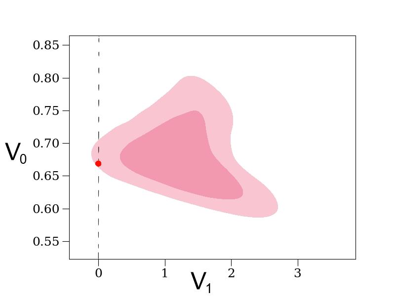
Figure 1: Distribution of parameter values $V_{0}$ and $V_{1}$ in a linear approximation to the scalar potential, with $\exp(-\chi^{2}/2)$ likelihood function computed by comparing model predictions to redshift vs brightness data in the Pantheon+ supernova catalogue (68 % and 95 % contours shown). Best fit $\Lambda$CDM model is indicated in red. Positive $V_{1}$ (corresponding to decreasing potential energy at present in our conventions) accounts for $>99\%$ of the distribution. Here, $V$ is normalized so that $V_{0}=\Omega_{\Lambda}$ in a $\Lambda$CDM model with $V_{1}=0$, and we are using units where $8\pi G/3=1$.

We begin in Section 2 with some theory. Starting from the Friedmann equation and scalar field evolution equation, we show how the time-dependence of scalar field potential and kinetic energies can be deduced from knowledge of the scale factor evolution together with the present densities of matter and radiation. For a single scalar field model in the approximation where radiation can be neglected, the evolution $a(t)$ together with $\Omega_{M}$ are enough to deduce both the scalar potential $V(\phi)$ and the time-dependence of the scalar field. Thus, assuming only a single scalar field, we in principle have direct access to its potential via observations of $a(t)$ and $\Omega_{M}$.

In practice, $\Omega_{M}$ is only loosely constrained by direct observations so even with precise knowledge of the scale factor evolution, we could only pin down the potential to within a one-parameter family. Even fixing $\Omega_{M}$, we find that small changes in the scale factor can correspond to significant changes in the potential. As a result, we will find that the modest uncertainties present in the supernova data and the associated scale factor evolution lead to much larger uncertainties in the deduced scalar potential. Indeed, we will find that while the $\Lambda$CDM model with no scalar field evolution provides a good fit to the data, typical models that provide a good fit have significant scalar field evolution and ${\cal O}(1)$ changes in the scalar potential $V(\phi)$ during the period $z\lesssim 2$ corresponding to the supernova data.

In Section 3, we describe the procedure to constrain model parameters based on the supernova data. For a given scalar potential $V(\phi)$, the potential parameters together with $\Omega_{M}$ and $H_{0}$ determine a scale factor evolution $a(t)$ and thus a theoretical redshift vs brightness curve that can be compared with supernova data. For each set of model parameters, we can calculate a chi-squared value, following precisely the same methodology as the Pantheon+ cosmology analysis in brout2022pantheon+ . The chi-squared values are used to define a likelihood function (a relative probability for the parameter values) and we use a Markov Chain Monte Carlo (MCMC) algorithm to sample from the resulting probability distribution, yielding histograms and correlation plots for the various parameters. As a check, we have verified that our code accurately reproduces the distribution obtained in brout2022pantheon+ for the $w$CDM model.

In Section 4, we present our results for parameter constraints in time-dependent scalar field models. We begin in Section 4.1 by considering models with a linear potential $V(\phi)=V_{0}+V_{1}\phi$, which we can think of as the first-order Taylor series approximation to a more general potential expanded about the present value of the scalar field. Such an approximation will always be valid over sufficiently short time scales, though not necessarily over the range of times corresponding to the supernova data. Our results for the parameter constraints in this class of models are displayed in Figures 3 and 4. We find that a large majority of the models providing a good fit to the data have a scalar potential that is presently decreasing with time. According to the $e^{-\chi^{2}/2}$ likelihood, $\approx 99.1\%$ of the distribution has $V_{1}>0$ ($\phi$ is presently decreasing with time according to our conventions), with $V_{1}\in[0.72,1.77]$ accounting for 68%. The scalar potential typically changes by a significant amount during the recent evolution, with $\langle|{\rm Range}[V(\phi(t))]/V(t_{0})|\rangle\approx 0.97$ over the time scale from which data is available ($z\lesssim 2$). In these models, the scalar potential energy will become negative at some time in the future; we find that the median time for this is $\sim 1.1$ Hubble times or $\sim 15$ billion years.

According to these results, the $\Lambda$CDM model (corresponding to $V_{1}=0$ and $V_{0}=1-\Omega_{M}$) sits relatively far out on the tail the distribution of allowed models with a linear potential (Figure 3). The parameter space includes models with all possible positive values of $\Omega_{M}$ up to about 0.35, while the $\Lambda$CDM model requires a much smaller range $\Omega_{M}=0.334\pm 0.018$. An independent estimation of $\Omega_{M}$ yielding a value less than 0.3 might thus naturally be explained by non-trivial scalar field evolution.

In Section 4.2, we extend the analysis to include a quadratic term in the potential. Here, we find a very large range of possible potentials that can provide a good fit to the data. In particular, essentially any value of the quadratic coefficient $V_{2}$ is allowed. The wide range of possible potentials can be understood based on certain approximate degeneracies in the parameter space. For large positive values of $V_{2}$, the scalar field can oscillate about the minimum of the potential. For $\sqrt{V_{2}}\gg H_{0}$, the scalar field evolution is well-approximated by a WKB solution, and the evolution of the energy density of such a solution in the Friedmann equation is the same as for non-relativistic matter turner1983coherent . Thus, we have an approximate degeneracy where a certain amount of matter is replaced by oscillating scalar field. For negative $V_{2}$, the scalar can spend a significant fraction of the evolution time close to the maximum of the parabolic potential, deviating from this value significantly only for early and/or late times. Again, the scale factor evolution can be similar to that of a $\Lambda$CDM model. Examples of very different scalar potential evolutions that all provide a good fit to the data are shown in Figure 6.

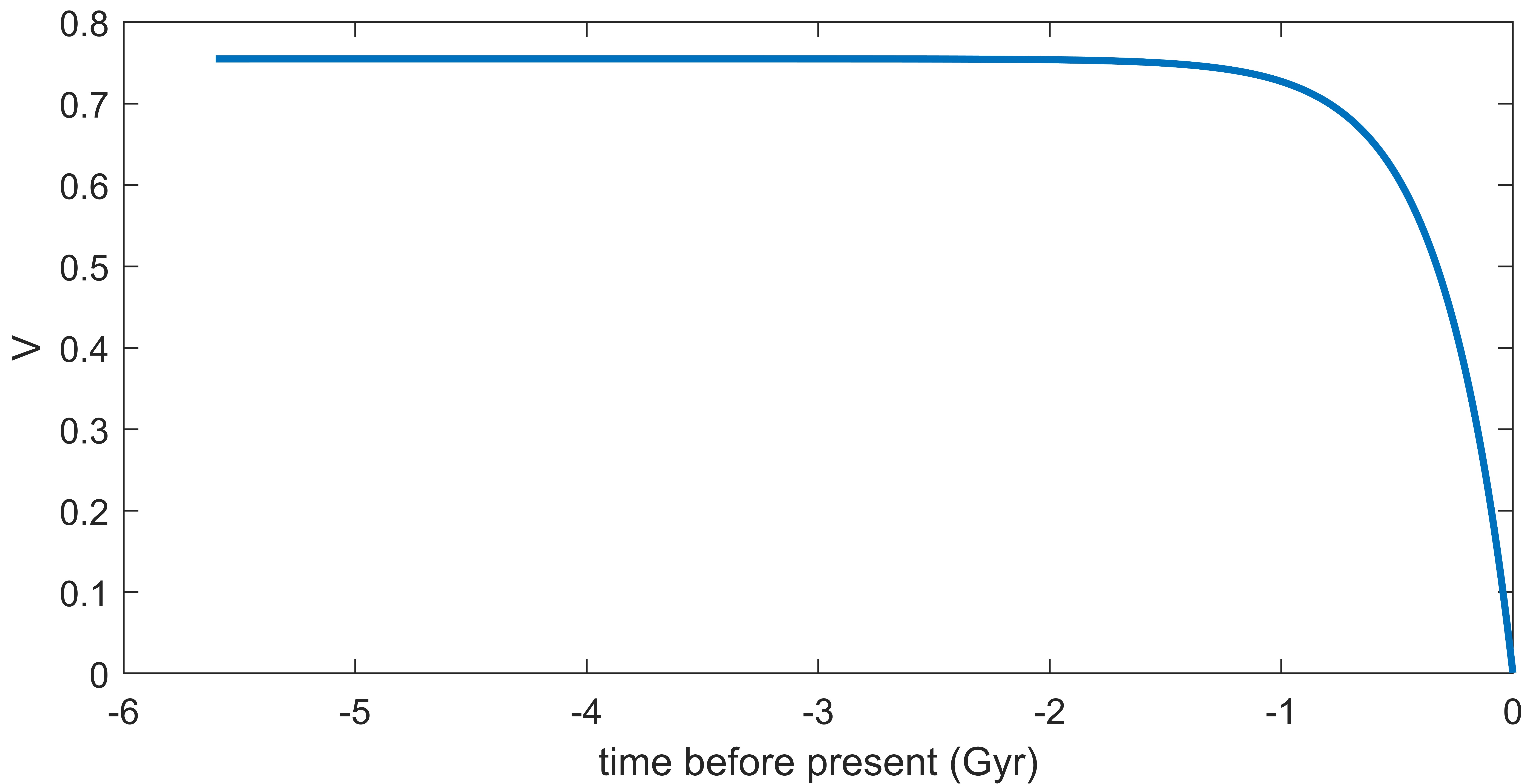
Figure 8: Scalar potential vs time for quadratic potential model providing the best fit to the Pantheon+ supernova data. The scalar field remains near the maximum of the potential until relatively recently.

A curious observation is that taking the full Pantheon+ data set, the best fit model with a quadratic potential has a downward-facing parabola, with the scalar sitting at the maximum of the potential ($V\approx 0.75$) until relatively recently ($t<2\textnormal{Gyr}$) before falling to almost precisely $V=0$ at the present time (Figure 8). In this model, the universe already stopped accelerating 400 million years ago! The model fits the data significantly better than $\Lambda$CDM ($\delta\chi^{2}\approx 17$), but the improvement is mainly related to the fit to very nearby supernovae ($z<0.01$) whose redshift/brightness relationship was noted in brout2022pantheon+ to deviate from the best fit $\Lambda$CDM model. These supernovae were mainly excluded in the analysis of brout2022pantheon+ , since the deviations from the model were argued to plausibly be due to some unmeasured local effect. For most of our analysis, we follow brout2022pantheon+ and include this $z<0.01$ cut. However, it seems worthwhile to note that if the $z<0.01$ deviations are in fact due to a cosmological effect, our model indicates that they might be explained by a late-time decrease in dark energy.

In summary, taking into account only the most direct measurements of the scale factor evolution, a rather significant variation of the scalar potential in the recent history of the universe appears to be allowed and within the approximation of a linear potential a scalar potential energy that is presently decreasing appears to be strongly preferred. Other observables will of course provide additional constraints on the model parameters but we have chosen to focus on supernova data for this study since these are the most straightforward to compare with the models without additional assumptions. It will be interesting to understand how significantly constraints from other existing data reduce the allowed parameter space.

2 Theory

In this section, we review some background material on cosmology with rolling scalar fields. Generally, the scalar potential together with the current densities of matter and radiation and the current Hubble constant determine the scale factor evolution $a(t)$ and the scalar field evolution $\phi(t)$ through the coupled Friedmann equation and scalar evolution equation. For a single scalar field model, we can also go the other way and deduce the scalar potential from the observed scale factor evolution and present matter/radiation densities.

2.1 Scalar potential from $a(t)$ and $\Omega_{M}$

Throughout our discussion we will assume a spatially flat FRW universe, with metric

$$ds^{2}=-dt^{2}+a(t)^{2}d\vec{x}^{2}\>,$$ (1)

and take the convention that the scale factor is $a=1$ presently. We focus on a model with a single scalar field $\phi$ with potential $V(\phi)$. Assuming that the scalar is minimally coupled to gravity (without curvature couplings), the evolution equation for the scalar field (assumed to be spatially constant) is

$$\ddot{\phi}+3H\dot{\phi}+V^{\prime}(\phi)=0\>,$$ (2)

where a dot denotes a $t$ derivative and $H=\dot{a}/a$ is the Hubble parameter. This is equivalent to the damped motion of a particle with position $\phi$ in a potential $V(\phi)$ with time-dependent damping parameter $3H(t)$. The gravitational equations yield the Friedmann equation

$$H^{2}={8\pi G\over 3}\left[\tilde{\rho}+{1\over 2}\dot{\phi}^{2}+V(\phi)\right]$$ (3)

where we define $\tilde{\rho}$ to be the energy density excluding that associated with the scalar field.

Taking the time derivative of the Friedmann equation and eliminating $\ddot{\phi}$ using the scalar equation gives an expression for the evolution of the scalar kinetic energy,

$${1\over 2}\dot{\phi}^{2}=-{1\over 8\pi G}\dot{H}+{1\over 6}a{d\tilde{\rho}\over da}\;.$$ (4)

Using this expression to eliminate the scalar kinetic energy in the Friedmann equation and solving the resulting equation for $V$ gives

$$V={1\over 8\pi G}\dot{H}+{3\over 8\pi G}H^{2}-\tilde{\rho}-{1\over 6}a{d\tilde{\rho}\over da}\>.$$ (5)

Thus, we can explicitly determine the evolution of scalar field kinetic and potential energies from knowledge of the scale factor evolution together with the present matter and radiation densities.

Evolution in the phase of matter and dark energy domination

For most of the history of the Universe, the cosmological expansion has (according to conventional models) been dominated by matter (including dark matter) and dark energy. Over this period, we have to a very good approximation that

$$\tilde{\rho}={\rho_{matter}^{now}\over a^{3}}={3H_{0}^{2}\Omega_{M}\over 8\pi G}{1\over a^{3}}\;,$$ (6)

where we are taking the usual definition

$$\Omega_{M}=\rho_{matter}^{now}{8\pi G\over 3H_{0}^{2}}$$ (7)

and $H_{0}$ is the present value of $\dot{a}/a$.

In this case, our equations (4) and (5) for the evolution of the scalar kinetic and potential energy become

$$K(t)\equiv{1\over 2}\dot{\phi}^{2}=-{1\over 8\pi G}\dot{H}-{3\over 16\pi G}\Omega_{M}H_{0}^{2}{1\over a^{3}}$$ (8)

and

$$V(t)={1\over 8\pi G}\dot{H}+{3\over 8\pi G}H^{2}-{3\over 16\pi G}\Omega_{M}H_{0}^{2}{1\over a^{3}}\>.$$ (9)

Thus, the scalar field potential and kinetic energy evolutions are determined completely by $a(t)$ and $\Omega_{M}$ in the approximation that we can ignore radiation.

The positivity of the kinetic energy at the present time gives a constraint

$$\Omega_{M}\leq-{2\over 3}{(\dot{H})_{0}\over H_{0}^{2}}={2\over 3}(1+q_{0})\;,$$ (10)

where

$$q_{0}=-\left(\frac{\ddot{a}a}{\dot{a}^{2}}\right)_{0}$$ (11)

is the “deceleration parameter”. The inequality becomes an equality if there is no scalar field kinetic energy, so for a given scale factor (e.g. deduced from observations) models with scalar fields will have a lower $\Omega_{M}$ than the standard $\Lambda$CDM model without scalars, assuming both fit the scale factor data. A measurement of the deceleration parameter thus provides a model-independent upper bound on the matter density (allowing arbitrary scalar fields and potentials). More generally, the positivity of scalar kinetic energy at general times implies that

$$\Omega_{M}\leq\min\left(-{2\over 3}{\dot{H}\over H_{0}^{2}}\right)\;,$$ (12)

where the minimum is taken over the range of times where we have reliable scale factor data.

Deducing the potential

Using the equation (8) for the scalar kinetic energy, we can take the square root and integrate, to obtain

$$\phi(t)=\phi(t_{0})+\int_{t_{0}}^{t}d\hat{t}\sqrt{-{1\over 4\pi G}\dot{H}(\hat{t})-{3\over 8\pi G}\Omega_{M}H_{0}^{2}{1\over a^{3}(\hat{t})}}\>,$$ (13)

where $t_{0}$ represents the present time, and we have chosen (without loss of generality) the convention that the scalar field is increasing its value at present. Since we also have

$$V(t)={1\over 8\pi G}\dot{H}+{3\over 8\pi G}H^{2}-{3\over 16\pi G}\Omega_{M}H_{0}^{2}{1\over a^{3}}\;,$$ (14)

we can combine (13) and (14) to parametrically define $V(\phi)$. Thus, observations of $a(t)$ and $\Omega_{M}$ determine in principle the part of the scalar potential over which the scalar varies during the time for which $a(t)$ is known. If we know $a(t)$ but not $\Omega_{M}$, we have a one-parameter family of possible potentials that can reproduce this, where the parameter is the value of $\Omega_{M}$. As an example, scalar field evolution in the potentials shown in Figure 2 with $\Omega_{M}=0.3,0.25,0.2,0.15$ and $0.1$ gives precisely the same scale factor evolution as the best fit $\Lambda$CDM model with $\Omega_{M}=0.334$. Details of this calculation are in Appendix A. This highlights that, to the extent the supernova data is well fit by a $\Lambda$CDM model, it is also well fit by other models with significant variation of $V$ during the recent cosmological history.

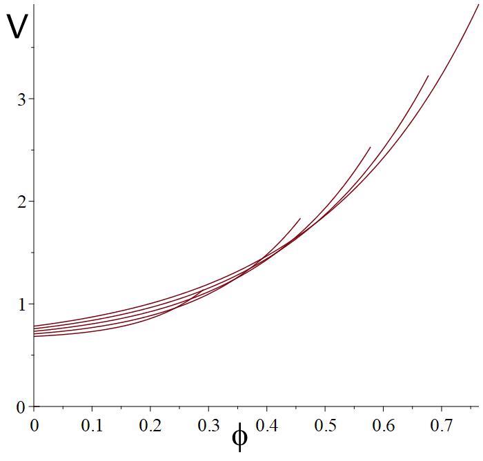
Figure 2: Potential $V(\phi)$ required to reproduce the $\Lambda$CDM fit to the observed scale factor back to $a=0.33$ ($z\approx 2$) in units with $8\pi G/3=1$. We use the $\Lambda$CDM value $\Omega_{M}^{0}=0.334$ and plot the potentials required if $\Omega_{M}=0.3,0.25,0.2,0.15$ and $0.1$ (bottom to top at the left). The scalar rolls from right to left, with the leftmost value representing the present time.

Rescaled variables

In the transformation from $a(t)$ to $V(\phi)$, a rescaling of time translates to an overall rescaling of the potential. Thus, we can think of the Hubble parameter $H_{0}$ as setting the overall scale of the potential, and the remaining shape of $a(t)$ as determining the shape of $V$. To highlight this, it is convenient to define rescaled quantities (we will suppress the tildes below and always refer to these)

$$s=H_{0}(t-t_{0})\>,\qquad\tilde{H}=\frac{H}{H_{0}}\>,\qquad\tilde{V}(\phi)=H_{0}^{-2}V(\phi)\>.$$ (15)

If we also work in units where $8\pi G/3=1$, the equations simplify to

$$\phi(s)=\phi(0)+\int_{0}^{s}ds_{1}\sqrt{-{2\over 3}{dH\over ds}-{\Omega_{M}\over a^{3}}}$$ (16)

and

$$V(s)={1\over 3}{dH\over ds}+H^{2}-{\Omega_{M}\over 2a^{3}}\;,$$ (17)

parametrically defining $V(\phi)$.

3 Observational data for scale factor evolution

We have seen in the previous section that precise knowledge of the scale factor evolution $a(t)$ together with $\Omega_{M}$ would allow us to reconstruct the scalar potential $V(\phi)$ and the scalar field evolution $\phi(t)$. We would now like to understand how the scalar potential and evolution are constrained by existing observations.

Model-independent measurements of $\Omega_{M}$

The mass density parameter $\Omega_{M}$ is rather weakly constrained if we don’t assume a cosmological model. For example, recent attempts at model-independent estimates are provided by the works Li:2019nux ; Ruiz-Zapatero:2022zpx that consider direct observations of the expansion and gravitational dynamics on the expanding background to place constraints on $\Omega_{M}$. The latter paper reports a range $\Omega_{M}=0.224\pm 0.066$. Allowing a 2 $\sigma$ range gives $\Omega_{M}\in(0.1,0.35)$, so it appears that the matter density parameter is only loosely constrained by direct observations. We will simply take $\Omega_{M}$ to be a free parameter in our models.

Measurements of $a(t)$

The most direct observations of the scale factor evolution come from redshift vs brightness observations of type Ia supernovae. The state-of-the-art compendium of carefully studied SNe Ia is the so-called Pantheon+ sample (2021) Pan-STARRS1:2017jku ; Scolnic:2021amr , which draws on observations from a number of independent surveys (including CfA, Pan-STARRS, Sloan Digital Sky Survey, Supernova Legacy Survey, Carnegie Supernova Project, Hubble Space Telescope, etc.). These comprise 1701 “spectroscopically confirmed” SNe Ia, between redshifts $z\approx 0$ and $z\approx 2.3$, with roughly a thousand SNe Ia at redshift $z>0.1$. This data has been used to constrain cosmological parameters Brout:2022vxf and the present Hubble constant Riess:2021jrx .

The supernova database provides results for observed magnitudes and redshifts of supernovae. Correcting for the effects of peculiar velocities (the velocities of objects relative to the cosmological background), the redshifts are related directly to the scale factor at the time of the supernova by

$$a=\frac{1}{1+z}\>.$$ (18)

The magnitudes are related fairly directly to luminosity distance $d_{L}$ (the distance that would be deduced from observed apparent magnitude and the presumed absolute magnitude assuming a time-independent flat geometry). This is algebraically related to the (positive) conformal time $\eta$ of the supernova (related to the usual cosmological time by $dt/a(t)=d\eta$) relative to the present time via

$$\eta=d_{L}/(1+z)\>,$$ (19)

Thus, the relation between $1/(1+z)$ and $d_{L}/(1+z)$ from supernova data can be considered as an observational picture of $a(\eta)$, the scale factor evolution in conformal time.

3.1 Constraining models based on supernova data

We would like to use the supernova data to constrain cosmological models with a single scalar field. For this, we follow the methodology of the Pantheon+ cosmology analysis.

The Pantheon+ supernova database provides values for redshift $z_{i}$ (corrected for known peculiar velocities) and a “distance modulus” $\mu_{i}$ deduced from the supernova light curve and related to the inferred luminosity distance by

$$\mu=5\log_{10}(d_{L}/10\textnormal{pc})\;.$$ (20)

For a choice of parameters $H_{0}$, $\Omega_{M}$, $V_{i}$, and $M$ we can obtain a model value $\mu_{i}$ for the redshift $z_{i}$ corresponding to each supernova by assigning a scale factor

$$a_{i}={1\over 1+z_{i}}$$ (21)

and numerically solving the coupled scalar evolution equations and Friedmann equations to determine $\eta(a)$ where we define $\eta$ to be the (positive) conformal time into the past in units of $1/H_{0}$. The relevant equations for the rescaled variables can be written in first order form as

$${d\phi\over da}=-{v_{\phi}\over aH}\qquad{dv_{\phi}\over da}={V^{\prime}(\phi)\over aH}-3{v_{\phi}\over a}\qquad{d\eta\over da}=-{1\over a^{2}H}\qquad H=\sqrt{{\Omega_{M}\over a^{3}}+{1\over 2}v_{\phi}^{2}+V(\phi)}$$ (22)

with boundary conditions

$$\eta(1)=0\qquad\phi(1)=0\qquad v_{\phi}(1)=\sqrt{2(1-\Omega_{M}-V(0))}\;.$$ (23)

The model value $\mu_{i}$ is then computed from (20), where using (19)

$$(d_{L})_{i}={\eta(a_{i})\over a_{i}H_{0}}\;.$$ (24)

To evaluate the fit of a certain set of model parameters, we calculate a $\chi^{2}$ value as

$$\chi^{2}=(\mu_{model}-\mu_{data})_{i}C^{-1}_{ij}(\mu_{model}-\mu_{data})_{j}$$ (25)

where $C$ is the covariance matrix provided by the Pantheon+ results that takes into account statistical and systematic error.

According to the standard analysis, the $\chi^{2}$ is used to assign a likelihood

$${\cal L}=e^{-\chi^{2}/2}$$ (26)

to a set of model parameters. We start from an assumed prior distribution of parameters which we take to be flat apart from the constraints $\Omega_{M}>0$ and $V_{0}+\Omega_{M}<1$, the latter required by the last equation in 22.

As described in the Pantheon+ cosmology analysis, the Hubble parameter $H_{0}$ is degenerate with another parameter $M$ that provides an overall additive correction to the average absolute magnitude of the supernovae (or a multiplicative correction to the brightness). In order to fix $H_{0}$ more precisely, the Pantheon+ analysis also considered a modified likelihood function which includes $M$ as an additional parameter and takes into account additional data from the SH0ES survey riess2022comprehensive for the distances to certain host galaxies deduced from using Cepheid variable stars as a standard candle. The modified $\chi^{2}$ is defined by replacing $(\mu_{model}-\mu_{data})_{i}$ in equation (25) with $(\mu_{Cepheid}-\mu_{data}-M)_{i}$ for supernovae in galaxies with an independent distance estimate and $(\mu_{model}-\mu_{data}-M)_{i}$ for others. In this case, the fit takes into account both how well the model matches with the supernova observations but also how well the supernova data match with the independent distance measure from the Cepheids.

We mention finally that the Pantheon+ analysis generally cut supernovae with $z<0.01$ from the analysis. This cut is motivated by the observation that the best fit $\Lambda$CDM models have residuals $\mu-\mu_{model}$ that are significantly positive on average for these nearby supernovae. This is taken to indicate the likely presence of some local effect (e.g. unmeasured peculiar velocities due to a local density excess) that has not been accounted for. We will generally follow the Pantheon+ analysis, making use of the Cepheid calibration and the $z<0.01$ cut. However, we also consider results coming from the complete data set.

As a check on our procedure, we performed an analysis of the $w$CDM model, finding distributions for parameters in excellent agreement with the Pantheon+ results in brout2022pantheon+ .

4 Results

In this section, we present our results for the parameter space of scalar potentials giving rise to scale factor evolution in good agreement with the supernova observations.

4.1 Linear potentials

We consider first a model with linear potential $V(\phi)=V_{0}+V_{1}\phi$. Even for a more complicated potential, expanding about the present value of $\phi$ will give this linear model for a short enough range of $\phi$, corresponding to some sufficiently small window of cosmological time. It is possible that this applies to the window $z<2$, but this is not necessarily the case; we extend the analysis to include quadratic terms in the potential in the next section. One motivation for studying the linear potential model is that it will give us an idea of how far we can deviate from a $\Lambda$CDM model while still obtaining a good fit to the data. In particular, it will provide a lower bound on the acceptable amount of variation of the potential energy during the evolution.

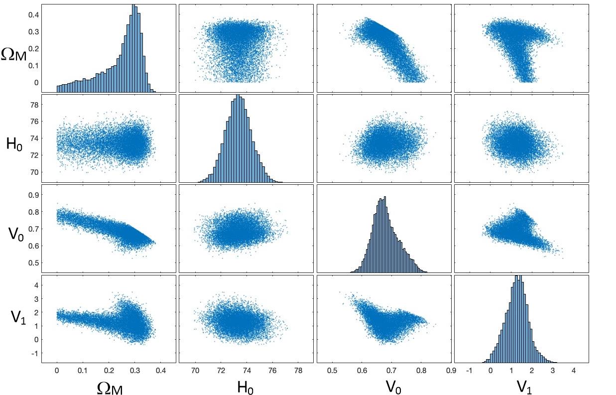
Figure 3: Distribution of parameter values $\Omega_{M}$, $H_{0}$, $V_{0}$, and $V_{1}$ for a linear potential scalar field model, using $e^{-\chi^{2}/2}$ likelihood calculated from Pantheon+ data calibrated with SHOES Cepheid distances. The $\Lambda$CDM model corresponds to $V_{0}=1-\Omega_{M}$, $V_{1}=0$.

In Figure 3, we show histograms and distributions for the parameters $\Omega_{M}$, $H_{0}$, $V_{0}$ and $V_{1}$, making use of the Cepheid data and the $z<0.01$ cut as in the Pantheon+ analysis. We are using the rescaled variables in which the potential is normalized as $V\to V/H_{0}^{2}$ so that $V_{0}=\Omega_{\Lambda}$ in a $\Lambda$CDM model. We are taking units with $8\pi G/3=1$ so $V_{1}$ of order 1 means that the rescaled potential changes by an order one amount when $\phi$ changes by a Planck scale amount.

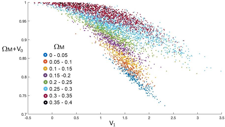
Figure 4: $\Omega_{M}+V_{0}$ vs $V_{1}$ for a linear potential scalar field model, using $e^{-\chi^{2}/2}$ likelihood calculated from Pantheon+ data calibrated with SH0ES Cepheid distances. The $\Lambda$CDM model corresponds to $V_{0}+\Omega_{M}=1$, $V_{1}=0$.

In Figure 4, we show $\Omega_{M}+V_{0}$ vs $V_{1}$, colour coded to show the $\Omega_{M}$ values. We see that the $\Lambda$CDM model, with $\Omega_{M}+V_{0}=1$ and $V_{1}=0$ is on the tail of the distribution defined by the $\exp(-\chi^{2}/2)$ likelihood. Models in the distribution typically have a significant variation in the scalar potential energy over the time range corresponding to the data: on average, we find $\textnormal{Range}[V(\phi)]/V_{0}\approx 0.97$ so there is typically an ${\cal O}(1)$ variation in the potential during the evolution for models that provide a good fit to the data. For linear potential models, the potential will eventually descend to negative values. Based on the distribution produced by our MCMC sampling, we find that the medial time for this to happen is approximately 1.1 Hubble times, a little larger than the current age of the universe.

From Figure 4 we see that there appear to be two different branches of allowable model parameters at larger $V_{1}$. The upper branch reaching the largest values of $V_{1}$ corresponds to models where $\phi$ first moves upward on the potential and then falls back down. In the lower branch (corresponding to small $\Omega_{M}$ values), the evolution of $\phi$ is monotonic, with $V$ monotonically decreasing.

We find that the marginalized distribution for $V_{1}$ has average value $V_{1}\approx 1.3$ with the range $V_{1}\in[0.72,1.77]$ containing 68% of the distribution with an equal amount above and below. We find 99.1% of the distribution has $V_{1}>0$, so the $\Lambda$CDM model is somewhat disfavoured within this space of linear potential models. This becomes more pronounced if we take into account the full data set (without the $z<0.01$ cut). Here, we find a significantly larger average value $V_{1}\approx 2.0$ with 68% of the distribution in $[1.51,2.56]$ and $V_{1}>0$ for 99.7% of the distribution. The preference for non-zero $V_{1}$ is already visible in results wang2004current ; Sahlen:2006dn ; Huterer:2006mv based on older data sets, though the result is not nearly as significant.

For the present value of the rescaled potential (equal to $\Omega_{\Lambda}$ in a $\Lambda$CDM model), we find $V_{0}=0.681\pm 0.044$.

For the $\Omega_{M}$ parameter, we find 99% of the distribution lies in the range $\Omega_{M}\in[0,0.352]$. While the distribution is peaked near $\Omega_{M}=0.3$, similar to the $\Lambda$CDM value of $0.334$ using the same data, the distribution is very broad (see Figure 3) extending to $\Omega_{M}=0$ with significant weight.

Finally, for the Hubble parameter, we find $H_{0}=(73.3\pm 1.0)$ km/s/Mpc, in agreement with the Pantheon+ cosmology analysis brout2022pantheon+ .

4.2 Quadratic potentials

Next, we consider adding a quadratic term to the potential, taking $V(\phi)=V_{0}+V_{1}\phi+V_{2}\phi^{2}/2$. We can view this as including the next term in the Taylor series approximation to some more general potential about the present value of the scalar field. More generally, it will provide insight into the model behaviors that are possible with potentials that have a changing slope.

For the space of models with parameters $\Omega_{M},H_{0},V_{0},V_{1},V_{2}$ and the absolute brightness adjustment parameter $M$, we find that it is possible to obtain a good fit to the data (comparable to or better than the best fit $\Lambda$CDM model) for a large variety of potential parameters. In fact, the Markov Chain Monte Carlo analysis does not converge well since $V_{2}$ does not have a bounded range in models that provide a good fit to the data. A partial explanation is that starting from a $\Lambda$CDM model that provides a good fit to the data, we can set $V_{2}$ to whatever we want without any change in the evolution provided that the scalar field continues to sit at the extremum of the potential. However, we can also have models with non-trivial scalar evolution giving significant variation in the potential for essentially any $V_{2}$.

For large positive values of $V_{2}$, the scalar field can oscillate many times about the minimum of the potential. As we review in Appendix B below, such an oscillating scalar contributes to the energy density in the same way as non-relativistic matter plus a cosmological constant, up to corrections suppressed by powers of $H_{0}/\sqrt{V_{2}}$ turner1983coherent . For large negative values of $V_{2}$, we can have a situation where the scalar spends a significant fraction of the time near the maximum of the potential, but changes significantly for early or late times.

The results of an MCMC analysis with the restriction $|V_{2}|<100$, are shown in Figure 5. The accumulation of points at larger $V_{2}$ values reflects the degeneracy of replacing matter with oscillating scalar. In Figure 6, we provide examples of various potentials and scalar evolutions that provide a fit to the data that is as good or better than $\Lambda$CDM. In Figure 7, we show the “equation of state parameter” $w=(\dot{\phi}^{2}/2-V)/(\dot{\phi}^{2}/2+V)$ as a function of the scale factor for several examples of models in our distributions for the linear potential and quadratic potential cases. We see a significant variety of behaviors here, so it is clear that the class of models we consider don’t map neatly onto the $w$CDM models (where $w(a)=w_{0}$) or $w_{0}w_{a}$CDM models (where $w(a)=w_{0}+w_{a}/a$) considered in brout2022pantheon+ and various other analyses.

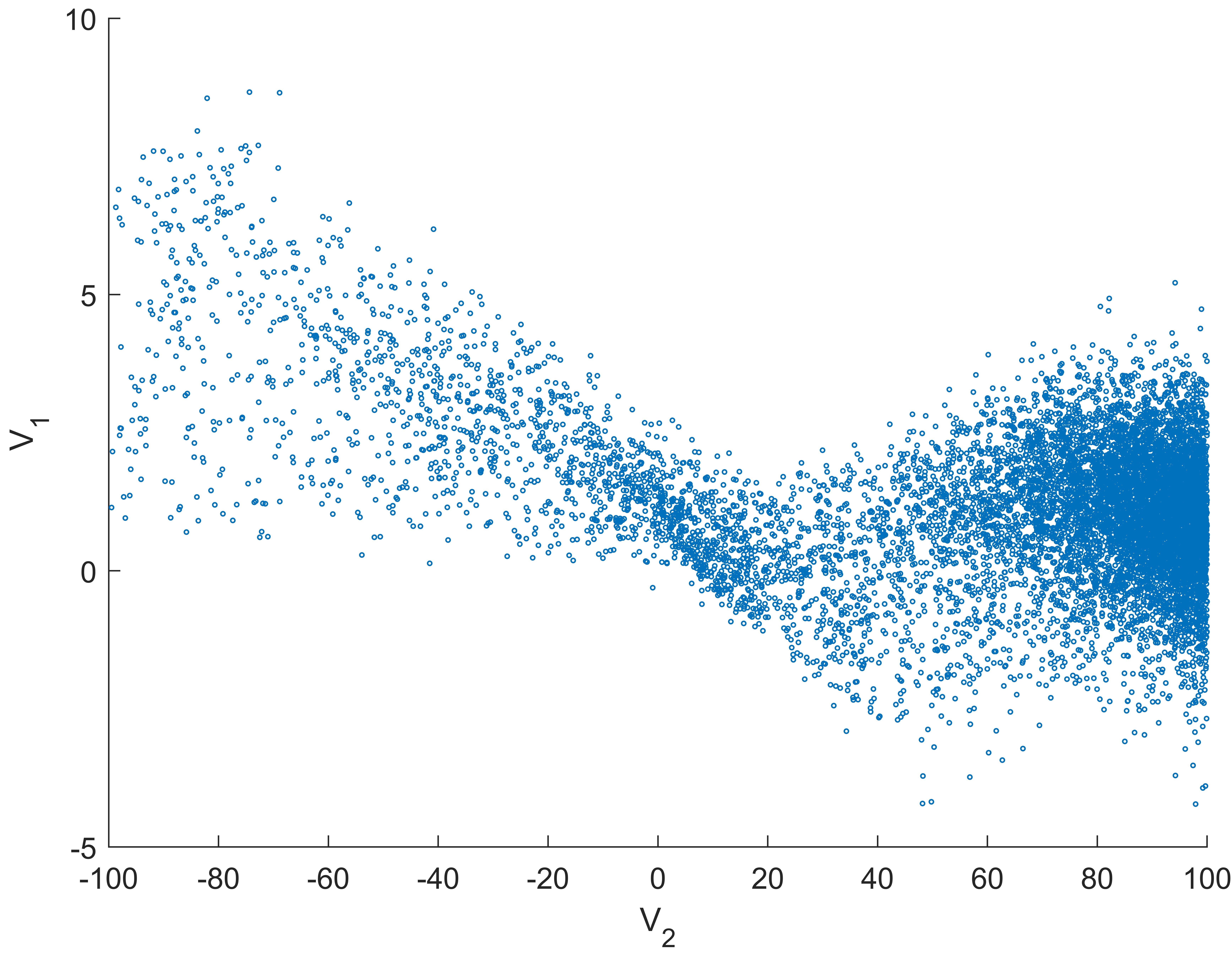
Figure 5: The ${\rm exp}(-\chi^{2}/2)$ distribution of potential parameters $V_{1}$ and $V_{2}$ for quadratic scalar potential model with restriction $|V_{2}|<100$. The large accumulation of points for larger $V_{2}$ is the result of a degeneracy where some amount of matter is replaced by scalar field oscillating in the quadratic potential.

Figure 6: Potentials $V(\phi)$ with corresponding scalar potential energy evolution $V(t)$ for various qualitatively different models providing a good fit to the supernova data. Time is measured in units of $1/H_{0}$.

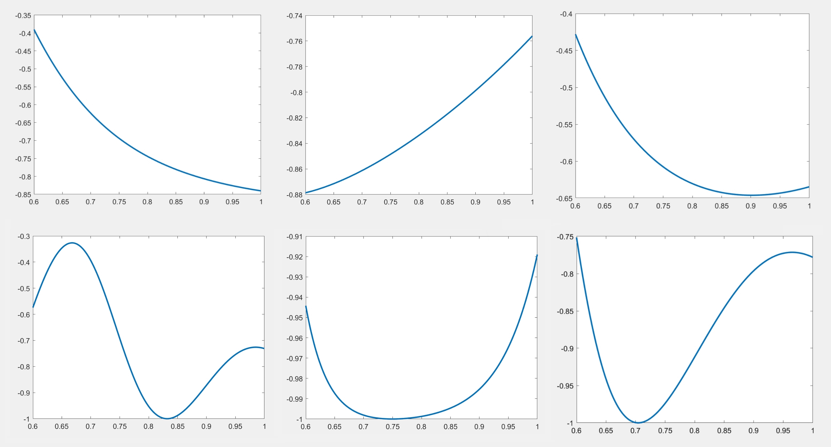
Figure 7: Equation of state parameter $w$ vs scale factor $a\in[0.6,1]$ for various models with a linear potential (top row) and a quadratic potential (bottom row), each providing a good fit to the supernova data.

A curious observation is that for the full Pantheon+ data set without the $z<0.01$ cut, the global best-fit model with quadratic potential (as far as we could tell) has

$$\Omega_{M}=0.339\qquad H_{0}=71.1\>\textnormal{km/s/Mpc}\qquad V_{0}=0.000845\qquad V_{1}=29.1\qquad V_{2}=-562.1$$ (27)

This provides a significantly better fit than $\Lambda$CDM ($\Delta\chi^{2}\approx 17$). For these parameters, the scalar remains near the maximum of the downward parabola until relatively late times ($\sim$1 Gyr before present) before descending to a value of nearly $V=0$ at present (the potential becomes negative within ${\cal O}(10^{5})$ years). In this model, the universe actually stopped accelerating 0.4 Gyr ago! That the present value of the potential is so nearly $V=0$ would seem to be purely a coincidence.

With the $z<0.01$ cut, the advantages of this or similar models over $\Lambda$CDM become much less significant. A plausible explanation is that there is some unaccounted for local effect that makes the very nearby supernovae less reliable for deducing the recent scale factor evolution. In this case, the data would be expected to deviate from the correct model for background evolution, and the better fit for the quadratic potential model would simply be due to having extra parameters for the background evolution that can reproduce this local effect.

On the other hand, if the $z<0.01$ data are providing a good picture of the recent scale factor evolution, our observations with the quadratic potential model suggest that the discrepancy with the $\Lambda$CDM model for these recent data might be due to a recent decrease in the potential energy.

5 Discussion

In this paper, motivated by certain theoretical considerations suggesting that non-trivial scalar field evolution is natural, we have explored the extent to which our most direct observations of scale factor evolution are compatible with a varying dark energy arising from a time-dependent scalar field.

One main conclusion is that there is a lot of room for such models, and models that are consistent with observations are not necessarily close to $\Lambda$CDM. Within the space of models we consider, we have found that in models providing a good fit to the data, the scalar potential typically changes by an order one amount compared to its present value during the time scale corresponding to the supernova data, roughly half the age of the universe. In the context of models with a linear potential, a large majority of the models ($>99\%$) in the distribution defined by the $\exp(-\chi^{2}/2)$ likelihood have a potential that is presently decreasing with time. This strong preference for decreasing dark energy is somewhat surprising; one might have expected that if $\Lambda$CDM is actually the correct model, extending the parameter space to the linear potential models would yield a distribution with a similar fraction of models with $V_{1}<0$ and $V_{1}>0$. The dominance of $V_{1}>0$ models in our distribution could thus be a hint that the correct model is not $\Lambda$CDM but one with a decreasing dark energy.

For models with a quadratic potential, we find a variety of qualitatively different possibilities, including models where the scalar field is now descending a downward-pointing parabola and models where the scalar is oscillating in an upward-facing parabola. Again, the best fit model has a decreasing dark energy at late times. The simple model we consider could be extended in various ways, for example by considering multiple scalars possibly with a non-trivial metric on target space, or by considering non-minimal couplings to gravity.

Models with scalar fields varying on cosmological time scales introduce various other phenomenological constraints that must be satisfied. The quanta of such a field will be nearly massless and thus result in long range forces for any matter that they couple to. In order to avoid observed violations of the equivalence principle, couplings to ordinary matter should be extremely small, so there should be some theoretical explanation for why this would be the case. Such a small coupling may be more natural with a pseudoscalar axion-like field marsh2016axion .

An interesting general result is that with non-trivial scalar evolution, a much wider range of $\Omega_{M}$ values is possible, extending all the way down to $\Omega_{M}=0$ (though of course there are positive lower bounds based on other observations). An independent estimate of $\Omega_{M}$ suggesting $\Omega_{M}<0.3$ might thus be a strong suggestion of non-trivial scalar evolution.

Appendix A Reproducing the best fit $\Lambda$CDM scale factor with various $\Omega_{M}$

According to our results above, even a completely precise knowledge of $a(t)$ still leaves is with a one-parameter family of possible potentials, where the parameter is $\Omega_{M}$. To illustrate this point, we suppose in this section, that the scale factor is precisely the one arising from a $\Lambda$CDM model with the parameters ($\Omega_{M}^{0}=0.334$, $H_{0}=73.6km/s/Mpc$) that provide a best fit to the Pantheon+ supernova redshift vs brightness data, and deduce the scalar potentials that would reproduce this same scale factor for smaller values of $\Omega_{M}$.

The $\Lambda$CDM curve $a(t;\Omega_{M}^{0},H_{0})$ corresponding to our choice of parameters is determined via the Friedmann equation in the $\Lambda$CDM model by

$$\dot{a}=H_{0}\sqrt{(1-\Omega_{M}^{0})a^{2}+{\Omega_{M}^{0}\over a}}\;.$$ (28)

We can integrate to find $a(t)$.

Now we would like to understand the $V(\phi)$ required to reproduce this same $a(t)$ for a model with some smaller $\Omega_{M}$. Making use of the rescaled variables defined above, the equation (28) together with (16) and (17) gives

$$\frac{da}{ds} = \sqrt{(1-\Omega_{M}^{0})a^{2}+{\Omega_{M}^{0}\over a}}$$

$${d\phi\over ds} = {1\over a^{3\over 2}}\sqrt{\Omega_{M}^{0}-\Omega_{M}}$$

$$\tilde{V} = {1\over 2a^{3}}(\Omega_{M}^{0}-\Omega_{M})+(1-\Omega_{M}^{0})$$

Dividing the second equation by the first, we get a differential equation for $\tilde{\phi}$ in terms of $a$. We have finally

$$\phi(a) = \int_{a}^{1}d\hat{a}{\sqrt{\Omega_{M}^{0}-\Omega_{M}\over(1-\Omega_{M}^{0})\hat{a}^{5}+\Omega_{M}^{0}\hat{a}^{2}}}$$

$$\tilde{V} = {1\over 2a^{3}}(\Omega_{M}^{0}-\Omega_{M})+(1-\Omega_{M}^{0}).$$

These two equations determine $\tilde{V}(\phi)$ parametrically.

In Figure 2, we plot the deduced potentials for $\Omega_{M}=0.3,0.25,0.2,0.15$ and $0.1$. We see that for lower values of $\Omega_{M}$, a larger amount of scalar evolution is required to produce the same $a(t)$. Even for the slightly lower value $\Omega_{M}=0.3$, the scalar potential would have descended from a value 33 percent more than its present value since $z=2$ while for $\Omega_{M}<0.286$ the scalar potential reproducing $\Lambda$CDM must have descended from more than twice its present value during the time frame for which supernova observations are available.

The particular shape of the potential showing up in the examples of Figure 2 is related to the starting assumption that the actual scale factor is precisely that of a $\Lambda$CDM model. We will see that slightly different scale factors can give substantially different potentials.

Appendix B Non-relativistic matter from oscillating scalar via the WKB approximation

In this section, we explain why models with large $V_{2}$ and significant oscillation in the scalar field potential energy can provide scale factor evolution very similar to a $\Lambda$CDM model.

To begine, we note that the limit $\sqrt{V_{2}}/H_{0}\gg 1$ (in units with $8\pi G/3=1$) is a limit where the scalar field equation can be well-approximated by a WKB-like approximation. Specifically, after a redefinition

$$\phi=\psi-{V_{1}\over V_{2}}\;,$$ (29)

we can write the scalar field equation as

$${d^{2}\psi\over dw^{2}}=-p^{2}(w)\psi$$ (30)

where

$$a^{3}{d\over dt}={d\over dw}$$ (31)

and

$$p(w)=\sqrt{V_{2}}a^{3}(w)\;.$$ (32)

This is exactly the Schrödinger equation, where $p(w)$ is the classical momentum. This is large provided that $V_{2}$ is large, so we can approximate the solution by the standard WKB expression

$$\psi(w)={C\over\sqrt{p(w)}}e^{\pm i\int p(w)dw}\;.$$ (33)

Rewriting in terms of the original variables and taking a general real combination of the solutions, we get

$$\phi(t)=-{V_{1}\over V_{2}}+{C\over a^{3\over 2}(t)}\cos(\sqrt{V_{2}}t+\varphi)$$ (34)

Plugging back into the Friedmann equation, the contribution to the energy density from the scalar field becomes

$${1\over 2}\dot{\phi}^{2}+V(\phi)=\left(V_{0}-{1\over 2}{V_{1}^{2}\over V_{2}}\right)+{V_{2}C^{2}\over 2}{1\over a^{3}}+\dots$$ (35)

where the omitted terms are suppressed by powers of $1/\sqrt{V_{2}}$ (or $H_{0}/\sqrt{V_{2}}$ before rescaling) relative to the terms present. The leading terms here behave exactly as a cosmological constant $V_{0}-V_{1}^{2}/(2V_{2})$ plus non-relativistic matter density. Thus, to an approximation that becomes increasingly good for larger $V_{2}$, we can reproduce the dynamics of a $\Lambda$CDM model by replacing some of the matter with an oscillating scalar field.

That oscillating scalars in a quadratic potential can act like non-relativistic matter was explained originally in turner1983coherent , and studied in many later works. From the quantum field theory point of view, such oscillating fields can be understood as a coherent state of a large density of the massive scalar particles associated with this scalar. The energy density of these particles (or the oscillating field) will gravitationally interact with other matter and radiation and develop inhomogeneities as with ordinary matter, so provides an interesting candidate for dark matter (see urena2019brief for a recent review).

However, in order for the scalar to contribute to the background evolution as we have described or to act as dark matter, it is essential that the associated scalar particles are nearly stable; this requires extremely small couplings to other fields and may be more natural with a pseudoscalar axion-like particle.

References

- (1) S. Perlmutter, G. Aldering, G. Goldhaber, R. Knop, P. Nugent, P. G. Castro et al., Measurements of and from 42 high-redshift supernovae, The Astrophysical Journal 517 (1999) 565.
- (2) A. G. Riess, A. V. Filippenko, P. Challis, A. Clocchiatti, A. Diercks, P. M. Garnavich et al., Observational evidence from supernovae for an accelerating universe and a cosmological constant, The Astronomical Journal 116 (1998) 1009.
- (3) G. Obied, H. Ooguri, L. Spodyneiko and C. Vafa, De Sitter Space and the Swampland, 1806.08362.
- (4) U. H. Danielsson and T. Van Riet, What if string theory has no de Sitter vacua?, Int. J. Mod. Phys. D 27 (2018) 1830007, [1804.01120].
- (5) I. Bena, M. Graña and T. Van Riet, Trustworthy de Sitter compactifications of string theory: a comprehensive review, 2303.17680.
- (6) T. Banks and W. Fischler, An Holographic cosmology, hep-th/0111142.
- (7) A. Strominger, The dS / CFT correspondence, JHEP 10 (2001) 034, [hep-th/0106113].
- (8) M. Alishahiha, A. Karch, E. Silverstein and D. Tong, The dS/dS correspondence, AIP Conf. Proc. 743 (2005) 393–409, [hep-th/0407125].
- (9) V. Gorbenko, E. Silverstein and G. Torroba, dS/dS and , JHEP 03 (2019) 085, [1811.07965].
- (10) E. Coleman, E. A. Mazenc, V. Shyam, E. Silverstein, R. M. Soni, G. Torroba et al., de Sitter Microstates from and the Hawking-Page Transition, 2110.14670.
- (11) B. Freivogel, V. E. Hubeny, A. Maloney, R. C. Myers, M. Rangamani and S. Shenker, Inflation in AdS/CFT, JHEP 03 (2006) 007, [0510046].
- (12) P. McFadden and K. Skenderis, Holography for Cosmology, Phys. Rev. D81 (2010) 021301, [0907.5542].
- (13) S. Banerjee, U. Danielsson, G. Dibitetto, S. Giri and M. Schillo, Emergent de Sitter Cosmology from Decaying Anti–de Sitter Space, Phys. Rev. Lett. 121 (2018) 261301, [1807.01570].
- (14) L. Susskind, Black Holes Hint Towards De Sitter-Matrix Theory, 2109.01322.
- (15) E. Di Valentino, O. Mena, S. Pan, L. Visinelli, W. Yang, A. Melchiorri et al., In the realm of the Hubble tension—a review of solutions, Class. Quant. Grav. 38 (2021) 153001, [2103.01183].
- (16) P. J. E. Peebles and B. Ratra, Cosmology with a Time Variable Cosmological Constant, Astrophys. J. Lett. 325 (1988) L17.
- (17) B. Ratra and P. J. E. Peebles, Cosmological Consequences of a Rolling Homogeneous Scalar Field, Phys. Rev. D 37 (1988) 3406.
- (18) R. R. Caldwell, R. Dave and P. J. Steinhardt, Cosmological imprint of an energy component with general equation of state, Phys. Rev. Lett. 80 (1998) 1582–1585, [astro-ph/9708069].
- (19) K. Dutta, Ruchika, A. Roy, A. A. Sen and M. M. Sheikh-Jabbari, Beyond CDM with low and high redshift data: implications for dark energy, Gen. Rel. Grav. 52 (2020) 15, [1808.06623].
- (20) L. Visinelli, S. Vagnozzi and U. Danielsson, Revisiting a negative cosmological constant from low-redshift data, Symmetry 11 (2019) 1035, [1907.07953].
- (21) A. A. Sen, S. A. Adil and S. Sen, Do cosmological observations allow a negative ?, 2021.
- (22) M. Van Raamsdonk, Cosmology without time-dependent scalars is like quantum field theory without RG flow, 2211.12611.
- (23) S. Antonini, P. Simidzija, B. Swingle and M. Van Raamsdonk, Cosmology from the vacuum, 2203.11220.
- (24) J. M. Maldacena and L. Maoz, Wormholes in AdS, JHEP 02 (2004) 053, [hep-th/0401024].
- (25) B. McInnes, Answering a basic objection to bang / crunch holography, JHEP 10 (2004) 018, [hep-th/0407189].
- (26) S. Cooper, M. Rozali, B. Swingle, M. Van Raamsdonk, C. Waddell and D. Wakeham, Black Hole Microstate Cosmology, JHEP 07 (2019) 065, [1810.10601].
- (27) S. Antonini and B. Swingle, Cosmology at the end of the world, Nature Phys. 16 (2020) 881–886, [1907.06667].
- (28) M. Van Raamsdonk, Cosmology from confinement?, 2102.05057.
- (29) S. Antonini, P. Simidzija, B. Swingle and M. Van Raamsdonk, Cosmology as a holographic wormhole, 2206.14821.
- (30) D. Scolnic et al., The Pantheon+ Analysis: The Full Dataset and Light-Curve Release, 2112.03863.
- (31) Y. Wang, J. M. Kratochvil, A. Linde and M. Shmakova, Current observational constraints on cosmic doomsday, Journal of Cosmology and Astroparticle Physics 2004 (2004) 006.
- (32) M. Sahlen, A. R. Liddle and D. Parkinson, Quintessence reconstructed: New constraints and tracker viability, Phys. Rev. D 75 (2007) 023502, [astro-ph/0610812].
- (33) D. Huterer and H. V. Peiris, Dynamical behavior of generic quintessence potentials: Constraints on key dark energy observables, Phys. Rev. D 75 (2007) 083503, [astro-ph/0610427].
- (34) D. Brout, D. Scolnic, B. Popovic, A. G. Riess, A. Carr, J. Zuntz et al., The pantheon+ analysis: cosmological constraints, The Astrophysical Journal 938 (2022) 110.
- (35) C. Andrei, A. Ijjas and P. J. Steinhardt, Rapidly descending dark energy and the end of cosmic expansion, Proceedings of the National Academy of Sciences 119 (2022) e2200539119.
- (36) M. S. Turner, Coherent scalar-field oscillations in an expanding universe, Physical Review D 28 (1983) 1243.
- (37) E.-K. Li, M. Du, Z.-H. Zhou, H. Zhang and L. Xu, Testing the effect of on tension using a Gaussian process method, Mon. Not. Roy. Astron. Soc. 501 (2021) 4452–4463, [1911.12076].
- (38) J. Ruiz-Zapatero, C. García-García, D. Alonso, P. G. Ferreira and R. D. P. Grumitt, Model-independent constraints on m and H(z) from the link between geometry and growth, Mon. Not. Roy. Astron. Soc. 512 (2022) 1967–1984, [2201.07025].
- (39) Pan-STARRS1 collaboration, D. M. Scolnic et al., The Complete Light-curve Sample of Spectroscopically Confirmed SNe Ia from Pan-STARRS1 and Cosmological Constraints from the Combined Pantheon Sample, Astrophys. J. 859 (2018) 101, [1710.00845].
- (40) D. Brout et al., The Pantheon+ Analysis: Cosmological Constraints, 2202.04077.
- (41) A. G. Riess et al., A Comprehensive Measurement of the Local Value of the Hubble Constant with 1 km/s/Mpc Uncertainty from the Hubble Space Telescope and the SH0ES Team, 2112.04510.
- (42) A. G. Riess, W. Yuan, L. M. Macri, D. Scolnic, D. Brout, S. Casertano et al., A comprehensive measurement of the local value of the hubble constant with 1 km s- 1 mpc- 1 uncertainty from the hubble space telescope and the sh0es team, The Astrophysical Journal Letters 934 (2022) L7.
- (43) D. J. Marsh, Axion cosmology, Physics Reports 643 (2016) 1–79.
- (44) L. A. Urena-López, Brief review on scalar field dark matter models, Frontiers in Astronomy and Space Sciences 6 (2019) 47.