Mixing time for uniform sampling of bipartite graphs with fixed degrees using the trade algorithm

Abstract

Uniform sampling of bipartite graphs and hypergraphs with given degree sequences is necessary for building null models to statistically evaluate their topology. Because these graphs can be represented as binary matrices, the problem is equivalent to uniformly sampling $r\times c$ binary matrices with fixed row and column sums. The trade algorithm, which includes both the curveball and fastball implementations, is the state-of-the-art for performing such sampling. Its mixing time is currently unknown, although $5r$ is currently used as a heuristic. In this paper we propose a new distribution-based approach that not only provides an estimation of the mixing time, but also actually returns a sample of matrices that are guaranteed (within a user-chosen error tolerance) to be uniformly randomly sampled. In numerical experiments on matrices that vary by size, fill, and row and column sum distributions, we find that the upper bound on mixing time is at least $10r$, and that it increases as a function of both $c$ and the fraction of cells containing a 1. Graph, Markov chain, Mixing time, Network, Randomization

1 Introduction

Uniform sampling of bipartite graphs and hypergraphs with given degree sequences is necessary for building null models to statistically evaluate their topology [8, 14, 19]. Because these graphs can be represented as binary matrices, the problem is equivalent to uniformly sampling $r\times c$ binary matrices with fixed row and column sums. This more general problem arises not only in network science [20], but also in physics [2, 26, 24], mathematics [3], psychometrics [27], and ecology [17]. To state the problem formally: Let $\mathcal{M}$ be the space of all $r\times c$ binary matrices $\mathbf{M}_{1}...\mathbf{M}_{n}$ with row sums $R_{1}...R_{r}$, column sums $C_{1}...C_{c}$, and fill $f=\frac{\sum{R}}{rc}=\frac{\sum{C}}{rc}$. How can we randomly sample $\mathbf{M}\in\mathcal{M}$ with uniform probability?

Many different solutions to this problem have been proposed [21], including algorithms that rely on filling [6, 15, 22], swapping [7], sampling [1, 13] and annealing [5] methods. The current state-of-the-art is the ‘trade’ algorithm, which includes the curveball [25], fastball [16] and parallel I/O-efficient [11] implementations that vary in their computational details. When using the trade algorithm, it is necessary to know how many trades must be performed to ensure that the resulting matrix $\mathbf{M}$ is uniformly randomly sampled from $\mathcal{M}$ (i.e. the mixing time). Although the trade algorithm is known to sample uniformly at random [9] and to be rapidly mixing under certain circumstances [12], only rough heuristics for its mixing time exist [25].

In this paper, we propose a distribution-based method for estimating the trade algorithm’s mixing time, and for generating samples of matrices that are nearly guaranteed to be uniformly randomly sampled from $\mathcal{M}$. We use this method to estimate its mixing time under a range of dimensional and distributional conditions. Our numerical results suggest that the upper bound on mixing time is at least $10r$, and that it increases as a function of $c$ and $f$, but does not depend on the distributions of $R$ or $C$. Although a precise upper bound remains unknown, this distribution-based method provides a way of ensuring that each member of a sample generated using the trade algorithm is uniformly randomly sampled from $\mathcal{M}$.

2 Trade algorithm

2.1 Description

The trade algorithm involves taking a random walk of length $t$ in the state space $\mathcal{M}$ from an initial state $\mathbf{M}_{1}$ to an end state $\mathbf{M}_{t+1}$. In each step of this random walk, 1s and 0s are randomly swapped between two randomly chosen rows, preserving each column’s sum and both rows’ sums. This swapping process is known as a ‘trade’ because it mirrors two children trading baseball cards. It improves on earlier swap methods that exchange, for example a ${}^{0}_{1}~{}^{1}_{0}$ submatrix with a ${}^{1}_{0}~{}^{0}_{1}$ submatrix, because a single trade can swap many 1s and 0s. The trade algorithm’s random walk is a Markov chain that is known to be finite, irreducible, and aperiodic [9], and therefore to converge on the uniform distribution. This means that, given a sufficient number of steps or trades $t$, $\mathbf{M}_{t+1}$ is chosen uniformly at random from $\mathcal{M}$. However, the number of trades that are required – the mixing time of the trade algorithm – remains unknown.

Existing implementations of the trade algorithm differ primarily in their time complexity. For example, the original curveball [25] implementation runs in $O(n~{}log~{}n)$, while fastball [16] runs in $O(n)$, and further improvements are possible through parallelization and I/O-efficiency [11]. Despite these differences, all implementations rely on the same Markov chain process for uniformly randomly sampling $\mathbf{M}\in\mathcal{M}$. We use the fastball implementation to perform the analyses reported below, however the results are general to any implementation of the trade algorithm.

2.2 Prior work on mixing time

Except for very small $\mathcal{M}$, computing the exact mixing time of the trade algorithm is intractable [9]. Therefore, prior work has focused on estimating the mixing time via numerical experiments measuring the degree of matrix perturbation. Let the perturbation $p$ between two matrices $\mathbf{M}_{a}$ and $\mathbf{M}_{b}$ be $p(\mathbf{M}_{a},\mathbf{M}_{b})=\frac{\sum|\mathbf{M}_{a}-\mathbf{M}_{b}|}{rc}$. That is, the perturbation is the fraction of entries that differ between the two matrices.

To estimate mixing time, [25] computed $p(\mathbf{M}_{1},\mathbf{M}_{t+1})$ for a range of $t$, seeking to determine “the number of swap attempts necessary to maximally perturb a matrix.” They observed that for a $100\times 100$ matrix the perturbation reaches a stable maximum on average at $t=500$, leading them to speculate that the mixing time is approximately $5r$ and to use this heuristic in an initial implementation called curveball. This finding was independently replicated by [9] using the same methods in $10\times 10$ and $100\times 100$ matrices, and has also been used to compare the mixing times of trade and swap algorithms [10].

This prior work has provided some insight into the mixing time of trade algorithms, but it has two notable limitations. First, prior work has focused on identifying the number of trades needed to maximally perturb a matrix. However, the goal is not to maximally perturb a matrix, but rather to perturb a matrix so that it can be regarded as uniformly randomly sampled from $\mathcal{M}$. In the language of Markov chains, the mixing time is not the number of steps required to reach a state that is maximally distant from an initial state, but instead is the number of steps required to ensure that a random walk has an equal probability of ending at every state in the space. Importantly, although $\mathcal{M}$ includes elements that are highly perturbed relative to $\mathbf{M}_{1}$, it also includes elements that are only slightly perturbed, and indeed includes $\mathbf{M}_{1}$ itself. Second, prior work has focused on identifying the number of trades $t$ when $p(\mathbf{M}_{1},\mathbf{M}_{t+1})$ ‘stabilizes,’ but no formal test of stability is conducted. Instead, the estimated mixing time $t$ has been inferred from visual inspection of a line graph plotting $p$ against $t$.

3 A distribution-based approach to estimating mixing time

To overcome these limitations, we propose a distribution-based approach to estimating mixing time. This approach focuses not on the perturbation $p$ between two matrices, but instead on the distribution of perturbations between a reference matrix and all members of a set of matrices.

We first define a theoretical distribution. Let $P(\mathbf{M},\mathcal{M})=p(\mathbf{M},\mathbf{M}_{1})...p(\mathbf{M},\mathbf{M}_{n})$, that is, the perturbations between an initial state $\mathbf{M}$ and all states in the state space $\mathcal{M}$. $P$ follows some unknown distribution that characterizes $\mathcal{M}$ with respect to $\mathbf{M}$, and which reflects the fact that elements of $\mathcal{M}$ are located at varying distances from $\mathbf{M}$.

We now define an empirical distribution. Let $\mathcal{M}^{t}_{s}$ be a set of $s$ binary matrices $\mathbf{M}^{t}_{1}...\mathbf{M}^{t}_{s}$ obtained after performing $t$ trades on a starting matrix $\mathbf{M}$. Then let $P^{t}_{s}(\mathbf{M},\mathcal{M}^{t}_{s})=p(\mathbf{M},\mathbf{M}^{t}_{1})...p(\mathbf{M},\mathbf{M}^{t}_{s})$, that is, the perturbations between $\mathbf{M}$ and each of $s$ matrices generated from $\mathbf{M}$ by the trade algorithm after $t$ trades.

When no trades have been performed, $P^{0}_{s}=0...0$ because every matrix in $\mathcal{M}^{0}_{s}$ is identical to $\mathbf{M}$. After $t$ trades, $P^{t}_{s}$ follows some unknown distribution because each $\mathbf{M}^{t}_{s}\in\mathcal{M}^{t}_{s}$ is located somewhere in $\mathcal{M}$ at varying distances from $\mathbf{M}$.

When a sample of $s$ matrices is uniformly randomly sampled from $\mathcal{M}$, then $P^{t}_{s}\sim P$. Of course, the distribution of $P$ is unknown. However, we can approximate the number of trades needed to achieve this state (i.e. the mixing time) by observing when the distribution of $P^{t}_{s}$ stabilizes. Moreover, we can formally test its stability by comparing comparing $P^{t}_{s}$ to $P^{t+z}_{s}$ using the Kolmogorov–Smirnov (KS) test for the equality of distributions [18, 23], where $z$ is the required duration of stability.

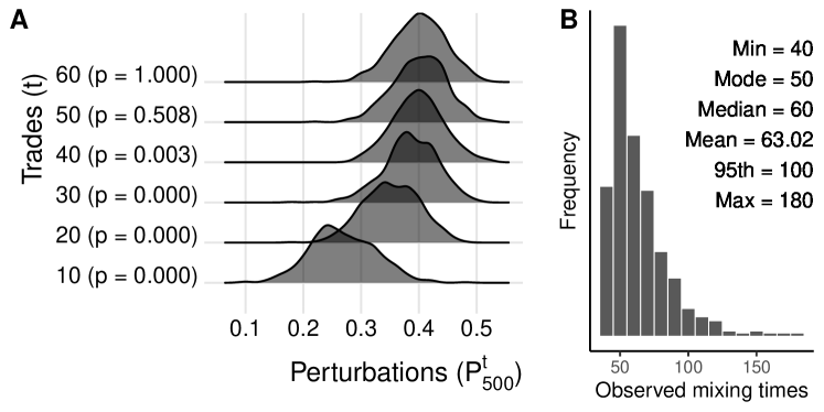
Figure 1: A distribution-based approach to computing mixing time. (A) The distribution of perturbations between a $10\times 10$ starting matrix and 500 matrices generated by the trade algorithm after $t$ trades. Each $p$-values test whether a distribution is the same as the previous distribution using the Kolmogorov–Smirnov test. (B) The distribution of observed mixing times over 500 replications.

Figure 1A offers a small illustration of this approach. We begin with a $10\times 10$ matrix $\mathbf{M}$ where $f=.5$ and both $R$ and $C$ are uniformly distributed. The bottom line shows the distribution of $P^{10}_{500}$, that is, the distribution of perturbations in 500 matrices generated by the trade algorithm after 10 trades. The associated $p$-value ($p<0.001$) indicates that it is statistically significantly different from the the distribution of $P^{0}_{500}$. The top line shows the distribution of $P^{60}_{500}$, that is, the distribution of perturbations in 500 matrices generated by the trade algorithm after 60 trades. The associated $p$-value shows that it is not statistically significantly different from the distribution of $P^{50}_{500}$. This means that after 50 trades the distribution of $P^{t}_{s}$ has stabilized, and therefore that this $\mathcal{M}^{50}_{500}$ can be regarded as a set of 500 matrices that have been uniformly randomly sampled from $\mathcal{M}$.

We call this value of $t=50$ the observed mixing time for these 500 random walks from this $\mathbf{M}$. However, starting from a different initial state, or even just taking different random walks from the same initial state, may have a different mixing time. Therefore, estimating the mixing time requires repeating the process illustrated in Figure 1A. Figure 1B shows the distribution of observed mixing times over 500 replications, each time starting from a $10\times 10$ matrix where $f=0.5$ and row and column sums are uniformly distributed. We find that for a matrix with these characteristics the most common mixing time is $t=50$, which matches the current $5r$ heuristic [25, 9]. However, we also find that the upper bound on this mixing time is substantially larger ($t=180$). While identifying the true upper bound may be important for theoretical reasons, for practical purposes of informing the use of the trade algorithm to generate random samples, the 95^th percentile offers a reasonable alternative. Here, we observe that the upper bound on mixing time, when applied to a $10\times 10$ matrix with $f=0.5$, is usually (i.e. 95% of the time) $t=100$.

There are several advantages to this distribution-based approach. First, because any given $\mathbf{M}\in\mathcal{M}$ may be similar or different from the initial state of the trade algorithm, it focuses on the distribution rather than the maximization of perturbation. Second, it offers a formal statistical test of a sample’s uniform randomness. Finally, and most practically, it actually returns a sample of matrices that is guaranteed (within the error of the KS test) to be uniformly randomly sampled from $\mathcal{M}$.

4 Numerical results

Figure 2 shows the results of using this distribution-based approach to estimate the upper bound on mixing time for matrices where the row and column sums have varying distributions (panel A), for maximally sparse matrices of varying dimensions (panel B), and for maximally dense matrices of varying dimensions (panel C). The R code necessary to reproduce these findings is available at https://osf.io/rmwpz/.

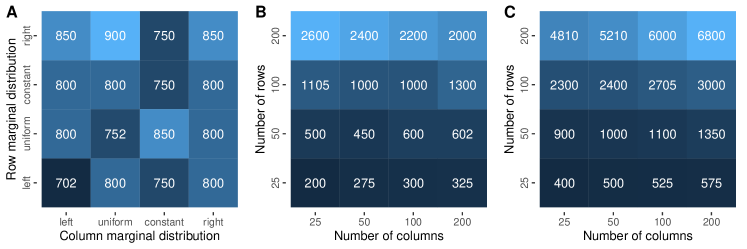
Figure 2: Estimated upper bound on mixing time of the trade algorithm for (A) $50\times 50$ matrices where $f=.1$ and the row and column sum have given distributions, (B) differing size matrices containing the minimum number of uniformly-distributed 1s, and (C) differing size matrices where $f=0.5$ and the row and column sums are uniformly distributed. Each value is the 95^th percentile, over 500 replications, of observed mixing times.

In each experimental condition, a sample of $s=500$ matrices is generated using the trade algorithm. This value ensures that the KS test is fully powered to detect cases where the test’s null hypothesis (i.e., that two distributions are the same) cannot be rejected at the $\alpha=0.05$ level, and therefore reduces the risk of type-II error [4]. The distribution of perturbations is evaluated after every $z=r$ trades. Choosing a lag parameter based on the matrix’s size recognizes that larger matrices require more trades to randomize, and therefore reduces the computational cost of estimating mixing time using this approach by reducing the frequency of computing perturbations and performing the KS test. The estimated upper bound on mixing time is the 95^th percentile of observed mixing times across 500 replications.

Figure 2A estimates the upper bound on mixing time for a $50\times 50$ matrix where $f=0.1$ and the row and column sums approximately follow one of four beta distributions: left-tailed ($\beta(10,1)$), uniform ($\beta(1,1)$), constant ($\beta(10000,10000)$), or right-tailed ($\beta(1,10)$). The estimated values are similar across all conditions, and there is no discernible pattern to the limited variation. This suggests that row and column sum distributions play a limited role in determining the upper bound on the mixing time of the trade algorithm.

Figure 2B shows estimated upper bound on mixing time for maximally sparse matrices that vary in size and that contain the fewest number of 1s to guarantee no empty rows or columns. Therefore $f$ varies from 0.005 for a $200\times 200$ matrix, to 0.04 for matrices where $min(R,C)=25$. Similarly, Figure 2C shows estimated upper bound on mixing time for maximally dense matrices that vary in size and where $f=0.5$. It is clear that the upper bound is always lower when $r\leq c$. Because the trade algorithm can simply be applied to a matrix’s transpose when $r>c$, we focus only on cases where $r\leq c$, which lie on or below the diagonal in both panels.

The values on the diagonal in Figure 2B suggest the upper bound on mixing time is at least $10r$, which is double the heuristic proposed by [25] for a matrix of arbitrary size and fill. Beyond this minimum, it increases as a function of $c$ and $f$. The upper bound we observe in these conditions closely follows $10r^{1+\frac{f}{2.5}+\frac{c}{125r}}$. This function is almost certainly overfitted and may not describe out-of-sample conditions, but suggests a possible functional form for the upper bound. In the absence of a precise upper bound on mixing time, the distribution-based approach used in these analyses offers a way to generate samples of matrices that are nearly guaranteeded to be unformly randomly sampled from $\mathcal{M}$

5 Conclusion

The trade algorithm is the state-of-the-art for uniformly randomly sampling bipartite graphs and hypergraphs with fixed degrees, and analogously sampling binary matrices with fixed row and column sums. However, its use in practice has been limited by the fact that its mixing time is unknown. We have proposed a distribution-based approach to studying its mixing time, and used this approach to estimate its upper bound. A series of numerical experiments suggest that the upper bound on mixing time is at least $10r$, and increases with the number of columns and the fraction of cells containing a 1.

Based on these results, we offer three recommendations for using the trade algorithm to uniformly randomly sample graphs or binary matrices. First, if the matrix is long (i.e., $r>c$), apply the trade algorithm to its transpose. Second, perform a minimum of $10r$ trades, but more if the matrix is wide (i.e., $c>r$) or not maximally sparse (i.e., $f>\frac{max(r,c)}{r\times c}$). Finally, when an appropriate number of trades is unknown, use the distribution-based approach described in section 3 to generate a sample that is nearly guaranteed to be uniformly randomly sampled from $\mathcal{M}$.

Data Availability

The R code necessary to reproduce these findings is available at https://osf.io/rmwpz/

References

- [1] Admiraal, R. & Handcock, M. S. (2008) Networksis: a package to simulate bipartite graphs with fixed marginals through sequential importance sampling. Journal of Statistical Software, 24(8).
- [2] Barré, J. & Gonçalves, B. (2007) Ensemble inequivalence in random graphs. Physica A: Statistical Mechanics and its Applications, 386(1), 212–218.
- [3] Barvinok, A. (2010) On the number of matrices and a random matrix with prescribed row and column sums and 0–1 entries. Advances in Mathematics, 224(1), 316–339.
- [4] Baumgartner, D. & Kolassa, J. (2021) Power considerations for Kolmogorov–Smirnov and Anderson–Darling two-sample tests. Communications in Statistics-Simulation and Computation, pages 1–9.
- [5] Bezáková, I., Bhatnagar, N. & Vigoda, E. (2007) Sampling binary contingency tables with a greedy start. Random Structures & Algorithms, 30(1-2), 168–205.
- [6] Blanchet, J. & Stauffer, A. (2013) Characterizing optimal sampling of binary contingency tables via the configuration model. Random Structures & Algorithms, 42(2), 159–184.
- [7] Boroojeni, A. A., Dewar, J., Wu, T. & Hyman, J. M. (2017) Generating bipartite networks with a prescribed joint degree distribution. Journal of Complex Networks, 5(6), 839–857.
- [8] Bruno, M., Saracco, F., Garlaschelli, D., Tessone, C. J. & Caldarelli, G. (2020) The ambiguity of nestedness under soft and hard constraints. Scientific Reports, 10(1), 1–13.
- [9] Carstens, C. J. (2015) Proof of uniform sampling of binary matrices with fixed row sums and column sums for the fast curveball algorithm. Physical Review E, 91(4), 042812.
- [10] Carstens, C. J., Berger, A. & Strona, G. (2018a) A unifying framework for fast randomization of ecological networks with fixed (node) degrees. MethodsX, 5, 773–780.
- [11] Carstens, C. J., Hamann, M., Meyer, U., Penschuck, M., Tran, H. & Wagner, D. (2018b) Parallel and I/O-efficient Randomisation of Massive Networks using Global Curveball Trades. In Azar, Y., Bast, H. & Herman, G., editors, 26th Annual European Symposium on Algorithms (ESA 2018), volume 112 of Leibniz International Proceedings in Informatics (LIPIcs), pages 11:1–11:15, Dagstuhl, Germany. Schloss Dagstuhl–Leibniz-Zentrum fuer Informatik.
- [12] Carstens, C. J. & Kleer, P. (2018) Speeding up switch Markov chains for sampling bipartite graphs with given degree sequence. In Approximation, Randomization, and Combinatorial Optimization. Algorithms and Techniques (APPROX/RANDOM 2018). Schloss Dagstuhl-Leibniz-Zentrum fuer Informatik.
- [13] Chen, Y., Dinwoodie, I. H. & Sullivant, S. (2006) Sequential importance sampling for multiway tables. The Annals of Statistics, 34(1), 523–545.
- [14] Cimini, G., Squartini, T., Saracco, F., Garlaschelli, D., Gabrielli, A. & Caldarelli, G. (2019) The statistical physics of real-world networks. Nature Reviews Physics, 1(1), 58–71.
- [15] Gale, D. et al. (1957) A theorem on flows in networks. Pacific Journal of Mathematics, 7(2), 1073–1082.
- [16] Godard, K. & Neal, Z. P. (2022) fastball: a fast algorithm to randomly sample bipartite graphs with fixed degree sequences. Journal of Complex Networks, 10(6), cnac049.
- [17] Gotelli, N. J. (2000) Null model analysis of species co-occurrence patterns. Ecology, 81(9), 2606–2621.
- [18] Kolmogorov, A. N. (1933) Sulla determinazione empirica di una legge didistribuzione. Giorn Dell’inst Ital Degli Att, 4, 89–91.
- [19] Neal, Z. P. (2022) backbone: An R package to extract network backbones. PloS one, 17(5), e0269137.
- [20] Neal, Z. P., Domagalski, R. & Sagan, B. (2021) Comparing Alternatives to the Fixed Degree Sequence Model for Extracting the Backbone of Bipartite Projections. Scientific Reports.
- [21] Penschuck, M., Brandes, U., Hamann, M., Lamm, S., Meyer, U., Safro, I., Sanders, P. & Schulz, C. (2020) Recent advances in scalable network generation. arXiv preprint arXiv:2003.00736.
- [22] Ryser, H. J. (1957) Combinatorial properties of matrices of zeros and ones. Canadian Journal of Mathematics, 9, 371–377.
- [23] Smirnov, N. (1948) Table for estimating the goodness of fit of empirical distributions. The annals of mathematical statistics, 19(2), 279–281.
- [24] Squartini, T., de Mol, J., den Hollander, F. & Garlaschelli, D. (2015) Breaking of ensemble equivalence in networks. Physical Review Letters, 115(26), 268701.
- [25] Strona, G., Nappo, D., Boccacci, F., Fattorini, S. & San-Miguel-Ayanz, J. (2014) A fast and unbiased procedure to randomize ecological binary matrices with fixed row and column totals. Nature Communications, 5(1), 1–9.
- [26] Touchette, H. (2015) Equivalence and nonequivalence of ensembles: thermodynamic, macrostate, and measure levels. Journal of Statistical Physics, 159(5), 987–1016.
- [27] Verhelst, N. D. (2008) An efficient MCMC algorithm to sample binary matrices with fixed marginals. Psychometrika, 73(4), 705–728.