Magnetic Fields of New CP Stars Discovered with Kepler Mission Data

Abstract

The paper presents the first results of the ongoing spectropolarimetric monitoring of magnetic fields of stars, whose chemically peculiar nature has been previously revealed with the 1-m SAO RAS telescope. We selected the sample candidates using the photometric data of the Kepler and TESS space missions. The efficiency of the method of searching for new CP stars based on photometric light curves has been confirmed. We present the magnetic field measurements and estimate the atmospheric parameters of the objects under study.

1 INTRODUCTION

Chemically peculiar (CP) stars of the upper part of the Main Sequence (MS) are characterized by the anomalous abundance of some chemical elements in the photosphere often unevenly distributed over the stellar surface. Among them, a group of magnetic chemically peculiar (mCP) stars stands out; it consists of classical Ap/Bp (CP2) stars and He-weak/rich (CP4) stars (Preston, 1974; Maitzen, 1984). These objects exhibit strictly periodic variations in brightness, spectral profiles, and magnetic fields; this can be explained in terms of the oblique rotator model of a rigidly-rotating star with stable spot structures on the surface and a stable global magnetic field that plays a stabilizing role (Deutsch, 1970).

Anomalies in the chemical element abundances of such objects arise as a result of long-term processes occurring in the outer calm atmospheric layers. The observed light variations are caused by the flux redistribution in spot structures due to the blanketing effect in the lines and continuum. The spots of chemical anomalies in the light curves usually appear bright in the optical domain and weak in the far UV, since this region contains many bound-bound and bound-free transitions of a number of elements (mainly Si, Fe, and rare-earth elements; see the paper by Krtička et al. (2012) and references therein for details). Despite the fact that mCP stars can be discovered in a fairly wide range of parameters of the Hertzsprung–Russell (HR) diagram, the occurrence of objects with detected magnetic fields remains almost constant and small for all types: about 10%, and the field properties do not demonstrate any pronounced dependences on mass, luminosity, or rotation (Wade et al., 2016; Schöllerr et al., 2017). The magnetic field is detected both in pre-MS objects (Kholtygin et al., 2019) and those being in the final stages of stellar evolution (Landstreet and Bagnulo, 2019). Evidence of evolutionary variations in the magnetic field during the MS stage were found by Semenko et al. (2022) when studying CP stars of the subgroups of different ages in the Orion OB1 association. Unfortunately, to date, the number of the known CP stars with a detailed modeling of the magnetic field structures is not enough to construct a complete model of its origin and subsequent evolution. This problem, in the authors’ opinion, is extremely interesting. To solve it, it is necessary to apply effective criteria for selecting the mCP-star candidates for subsequent observations with modern ground-based spectropolarimeters.

Until now, most CP stars have been identified as chemically peculiar using spectroscopic methods or, more rarely, using the $\Delta a$ photometry (Paunzen et al., 2005). Spectropolarimetry was used to measure the magnetic field. As a rule, photometric observations previously fulfilled an auxiliary role to refine the rotation periods mainly. The things changed after publications of the photometric archives of the Kepler, TESS, and other space missions. High precision, sufficient completeness of the time series and sky coverage of the surveys make it possible to use these data for solving a wide range of astronomical problems in addition to exoplanet detection including asteroseismological studies and rotational modulation of mCP stars (Hümmerich et al., 2018; David-Uraz et al., 2019; Mikulášek). Although the amplitude of the photometric variability of such stars is very small and usually does not exceed $0\hbox{$\,.\!\!^{\rm m}$}12$ in the $V$ band, the time series are more suitable for determining the rotation period than the spectra. The light curves of mCP stars are smooth and can be fit reasonably by a single or double wave (Mathys and Manfroid, 1985; Dukes and Adelman, 2018; Mikulášek et al., 2018). They are well approximated by a second-order polynomial which corresponds to the model of a rotating star with one or two large photometric spots. The shape and period of the light curves of CP stars persist for decades (Žižňovský, 1994). In the paper by Hümmerich et al. (2018), based on photometry from the Kepler satellite, several new CP stars were found and an unexpected variety of shapes of their light curves was shown. Using the spectra obtained with the 1-m Zeiss-1000 SAO RAS telescope, observations with the 60-cm telescope of the Stara Lesna observatory (Slovakia), and the LAMOST survey archive, the authors of the cited paper classified the peculiarity type of the sample objects and identified 39 new CP stars out of 46 photometric candidates (85%). The resulting list of CP stars became the basis for spectropolarimetric monitoring which has been carried out with the Main Stellar Spectrograph (MSS) of SAO RAS since 2019. In this paper, we present the first results of a comparative analysis of the variability of a number of CP stars that we have selected based on the photometric data from the Kepler satellite for spectropolarimetric monitoring at the 6-m BTA telescope and estimate their fundamental parameters.

2 SAMPLE SELECTION AND ANALYSIS TECHNIQUE

2.1 Selection Criteria

The selection of candidates for spectropolarimetric observations was carried out based on the photometric data from the Kepler mission according to the method proposed by colleagues from the Masaryk University, Brno (Hümmerich et al., 2018). When analyzing the time series, first of all, it is necessary to distinguish the rotational variability from the variability associated with the $\gamma$ Dor, $\beta$ Cep-type pulsations, slowly pulsating B stars, as well as with the orbital motion of the star; therefore, when compiling the sample, we used the following criteria:

• the early $B$ to early $F$ spectral type with corresponding color index or effective temperature (if available);

• the rotation period greater than 0$\,.\!\!^{\rm d}5$;

• the presence of a single frequency and the corresponding harmonics on the periodograms;

• the light curve is stable or varies slightly during the entire observation period;

• the variability amplitude does not exceed several hundredths of magnitude.

From the resulting list, we selected 10 candidates for subsequent spectropolarimetric monitoring with the BTA telescope. This sample includes both new CP star candidates and well-known mCP stars for the method checkout.

2.2 Photometric Data

In this paper, we used the data from the MAST archive obtained by the TESS (Transiting Exoplanet Survey Satellite) space telescope (Ricker et al., 2015) launched to search for exoplanets with the transit method. During the two-year period of the main program, the mission covered 85% of the whole sky carrying out observations in the overlapping sectors of the $96^{\circ}\times 24^{\circ}$ size. This made it possible to obtain photometric series for more than 470 million point sources. Depending on location, objects were observed on different time domains: from 27.4 days to almost 1 year. TESS was launched on April 18, 2018, and in December of the same year the data of the first two sectors became publicly available.

We analyzed the photometric time series using the Lafleur–Kinman method (Lafler and Kinman, 1965). The long-term trends associated with the technical issues caused that are inherent in the space telescope observations were preliminarily excluded.

The rotation periods from the TESS data are in good agreement with those published earlier in the paper by Hümmerich et al. (2018), where the photometric series of the Kepler mission were used for searching. Small differences in the fourth or fifth decimal place are inevitable when using different data sets and period search methods, their study is beyond the scope of this paper.

2.3 Spectropolarimetry

The observations were carried out with the MSS spectrograph (Panchuk et al., 2014) of the 6-m BTA telescope with a circular polarization analyzer (Chountonov, 2016) equipped with the $\lambda/4$ rotating phase plate. The E2V CCD42-90 CCD with a size of $4600\times 2000$ elements was used as a light detector. Each observation involves obtaining a pair of the Zeeman spectra with the plate rotated by 90^∘. Such a procedure allows one to exclude instrumental polarization and other technical issues that may cause false detection of a magnetic field. The exposure time was chosen so that the $S/N$ ratio in the spectra was at least 100. In each observation night, in addition to the study targets, the spectra of the standard stars were obtained: the stars with a well-known magnetic phase curves as well as the stars with zero magnetic fields.

The spectra were extracted using the software package written for the ESO MIDAS environment in SAO RAS (Kudryavtsev, 2000). The width of the observed range was 600 Å  in the interval of 4400–4900 Å. The choice of the range is determined by the presence of a sufficient number of lines inside it to measure a magnetic field with acceptable accuracy.

The magnetic field was measured according to the method proposed by Bagnulo et al. (2002). The longitudinal field measurement error is quite sensitive to the $S/N$ ratio, $FWHM$, and the profile of the measured spectral lines.

The atmospheric parameters were estimated using the SME software for calculating synthetic spectra (Piskunov and Valenti , 2017). By varying the effective temperature $T_{\rm eff}$, the surface gravity $\log g$, the radial velocity $V_{R}$, the rotation velocity projected on the line of sight $v_{e}\sin i$ and, if necessary, the metallicity $[{\rm M/H}]$, we achieved the best fit between the observed H${\beta}$ Balmer line and the synthetic spectrum. To build the last, we used the LLmodels model grid (one-dimensional plane-parallel atmosphere, the LTE approximation, the ‘‘line-by-line’’ approach to calculate the spectral line profiles) (Shulyak et al., 2004) and a list of lines obtained from the VALD database (Piskunov et al., 1995). Note that detailed modeling of the chemical abundance of objects is beyond the scope of this paper; here we restrict ourselves to only approximate estimation of parameters from the spectra we have.

To build the phase curve of the magnetic field, we used the found photometric periods, after which the resulting curves were approximated by one or the sum of two sinusoids. The zero phase of the photometric light curve corresponds to the maximum brightness of the series.

3 RESULTS

We estimated the reliability of detecting the magnetic field in the studied stars using the criterion of the reduced statistics of $\chi^{2}/n$ calculated with the formula:

$$\chi^{2}/n=\dfrac{1}{n}\sum_{i=1}^{n}\left(\dfrac{B_{i}}{\sigma_{i}}\right)^{2},$$

where $B_{i}$ and $\sigma_{i}$ are individual measurements of a magnetic field and the corresponding errors. Traditionally, as for our method (see, e.g., Romanyuk et al. (2019)), we will assume that the magnetic field is reliably detected at $\chi^{2}/n>5$.

The results of individual magnetic measurements of the sample objects are given in Table LABEL:tab:log1, where JD is a Julian date of observations, $B_{e}\pm\sigma$ is the estimation of the longitudinal magnetic field and the corresponding root-mean-square error. Below we give the comments on the results obtained during the study.

3.1 KIC 4180396 = HD 225728

Analysis of the TESS photometric data has shown that the observations of the object are best described by the following ephemeris:

$${\rm JD}=2455684.20056+3.68435E.$$

Figure 1a shows the resulting light curve. It exhibits a double wave with the primary maximum and minimum at the rotation period phases: $\phi=0.0$ and $\phi=0.28$. They are followed by the secondary maximum and minimum at the phases: $\phi=0.52$ and $\phi=0.78$ respectively. The full amplitude of the light variation is equal to $\Delta m=0\hbox{$\,.\!\!^{\rm m}$}013$. The positive magnetic extremum $B_{e}{\rm(max)}=1520\,\pm\,52$ G, corresponds to the photometric maximum. The negative extremum of the field is slightly shifted relative to the secondary photometry maximum towards the primary minimum and is in the phase $\phi=0.2$. The field is best approximated by a double sine curve (Fig. 1b), while the secondary harmonics are almost invisible. The estimate $\chi^{2}/n=319.8$ confirms reliable detection of the magnetic field.

As a result  of the  spectrum  approximation (see Fig. 1c) the following atmospheric parameters are defined: $T_{\rm eff}=11\,283$ K, $\log g=3.80$, $v_{e}\sin i=28.67$ km s^-1, $V_{R}=-8.65$ km s^-1, and $[{\rm M/H}]=-0.096$.

3.2 KIC 5264818 = HD 180374

The best ephemeris that we obtained as a result of the photometric series analysis:

$${\rm JD}=2458683.9789+1.90291E.$$

Table 1: Longitudinal magnetic fields of the sample stars according to our measurements

Star	JD 2450000+	$B_{e}\pm\sigma$, G
KIC 4180396	8578.553	$-$544$\,\pm\,$	70
	8603.478	$-$650$\,\pm\,$	75
	8777.274	$-$578$\,\pm\,$	70
	8802.198	$-$250$\,\pm\,$	80
	8805.222	1517$\,\pm\,$	80
	9033.494	1400$\,\pm\,$	70
	9099.448	1520$\,\pm\,$	70
KIC 5264818	8597.496	1004$\,\pm\,$	65
	8621.370	$-$995$\,\pm\,$	70
	8624.414	227$\,\pm\,$	70
	8777.211	$-$810$\,\pm\,$	80
	8778.165	940$\,\pm\,$	70
	8921.519	300$\,\pm\,$	50
	9001.340	960$\,\pm\,$	50
	9006.387	101$\,\pm\,$	65
	9032.509	$-$566$\,\pm\,$	50
	9061.482	$-$629$\,\pm\,$	50
	9097.388	$-$757$\,\pm\,$	55
KIC 5473826	8600.401	$-$701$\,\pm\,$	203
	8801.276	99$\,\pm\,$	205
	8805.194	$-$286$\,\pm\,$	120
	9031.340	$-$479$\,\pm\,$	180
	9096.346	$-$147$\,\pm\,$	143
KIC 6065699	8577.541	650$\,\pm\,$	80
	8620.381	563$\,\pm\,$	50
	8621.438	550$\,\pm\,$	122
	8624.481	463$\,\pm\,$	80
	8777.330	731$\,\pm\,$	60
	8778.336	676$\,\pm\,$	70
	8799.281	781$\,\pm\,$	63
	8802.254	720$\,\pm\,$	46
	8805.149	820$\,\pm\,$	60
	9006.424	539$\,\pm\,$	70
	9060.308	445$\,\pm\,$	70
	9061.535	691$\,\pm\,$	74
	9102.403	845$\,\pm\,$	90
KIC 6278403	8601.473	$-$220$\,\pm\,$	90
	8603.420	$-$179$\,\pm\,$	90
	8620.434	$-$130$\,\pm\,$	90
	8621.411	171$\,\pm\,$	90
	8624.453	63$\,\pm\,$	90
	9006.365	10$\,\pm\,$	90
	9097.367	$-$20$\,\pm\,$	90
	9431.500	100$\,\pm\,$	100
KIC 6864569	8758.312	$-$195$\,\pm\,$	70
	8778.297	16$\,\pm\,$	80
	8830.141	$-$305$\,\pm\,$	85
	9060.502	$-$403$\,\pm\,$	53
	9455.439	177$\,\pm\,$	91
KIC 8161798	8600.490	$-$50$\,\pm\,$	100
	8802.151	$-$55$\,\pm\,$	100
	8830.205	250$\,\pm\,$	100
	9032.464	240$\,\pm\,$	100
	9060.416	$-$157$\,\pm\,$	100
	9096.433	118$\,\pm\,$	100
	9336.542	210$\,\pm\,$	100
	9455.347	$-$105$\,\pm\,$	100
KIC 8324268	8577.516	135$\,\pm\,$	90
	8600.558	$-$7$\,\pm\,$	90
	8601.559	$-$11$\,\pm\,$	90
	8620.353	$-$450$\,\pm\,$	90
	8624.504	$-$185$\,\pm\,$	90
	8777.352	0$\,\pm\,$	90
	8778.360	460$\,\pm\,$	90
	8799.233	$-$190$\,\pm\,$	90
	8801.326	$-$170$\,\pm\,$	90
	8805.305	$-$227$\,\pm\,$	90
	9000.368	$-$117$\,\pm\,$	90
	9021.410	$-$20$\,\pm\,$	90
	9096.534	$-$150$\,\pm\,$	90
KIC 10324412	8620.323	50$\,\pm\,$	55
	8621.336	2$\,\pm\,$	70
	8624.377	$-$101$\,\pm\,$	70
	8799.259	$-$103$\,\pm\,$	90
	8801.153	$-$5$\,\pm\,$	60
	8976.335	$-$65$\,\pm\,$	70
	9061.456	$-$23$\,\pm\,$	170
	9097.416	$-$164$\,\pm\,$	122
	9099.397	$-$72$\,\pm\,$	80
	9455.276	$-$138$\,\pm\,$	127
KIC 11560273	8758.257	0$\,\pm\,$	100
	8777.375	$-$48$\,\pm\,$	90
	8778.387	$-$17$\,\pm\,$	100
	8830.260	40$\,\pm\,$	100
	9061.532	56$\,\pm\,$	100

Table 1: (Continued)

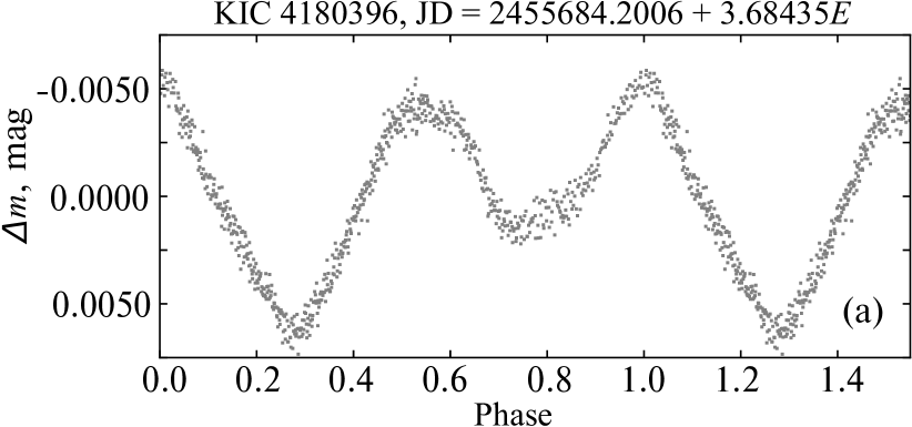
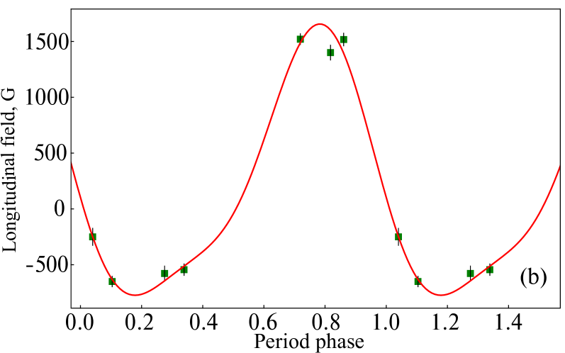
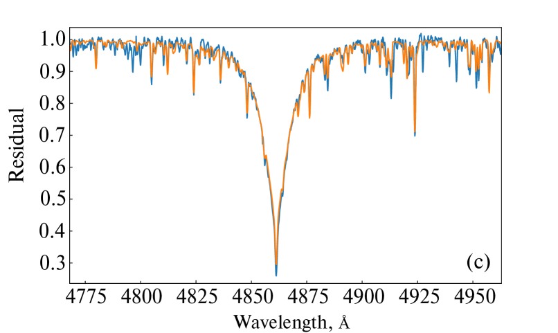
Figure 1: Analysis of the star KIC 4180396. Panel (a) shows the light curve according to the TESS satellite data; panel (b) shows the phase curve of the magnetic field; panel (c) presents the modeling result of the H${\beta}$ line, observations are shown in blue, and modeling results in orange.

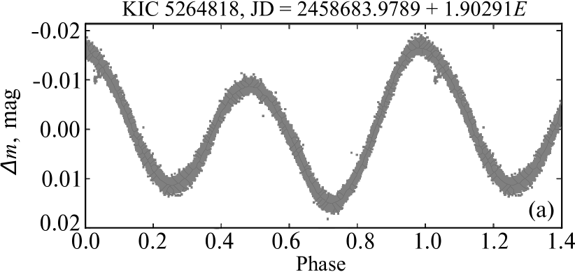
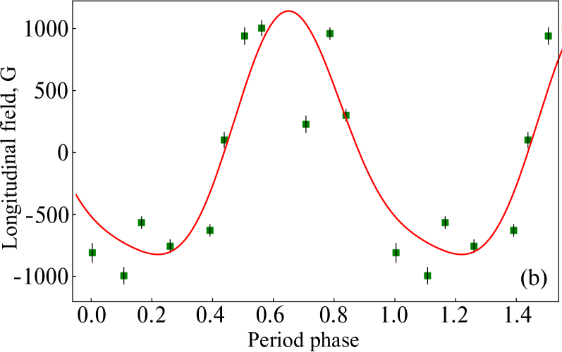
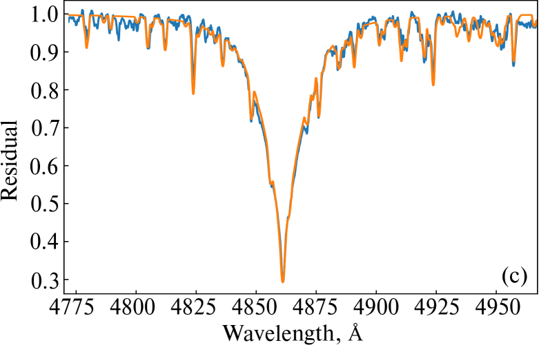
Figure 2: Same as in Fig. 1, for KIC 5264818.

The light curve (Fig. 2a) has a more pronounced double wave. The primary maximum is followed by the secondary minimum and maximum in the phases: $\phi=0.25$ and $\phi=0.50$. Further, the primary minimum is in the region of the phase $\phi=0.73$. The full amplitude is equal to $\Delta m=0\hbox{$\,.\!\!^{\rm m}$}037$.

The positive magnetic field extremum lies in the region of the primary minimum of the light curve; it is slightly shifted relative to it in the phase $\phi=0.61$. The negative field maximum is flat and located between the primary maximum and the secondary minimum of photometry in the range of the phases $\phi:\leavevmode\nobreak\ 0.0$–$0.22$. The magnetic field is best approximated by a double sine curve (see Fig. 2b). The star KIC 5264818 is reliably magnetic ($\chi^{2}/n=146.9$).

With the approximation of the spectrum  shown in Fig. 2c, the following  atmospheric  parameters  are  obtained: $T_{\rm eff}=9348$ K, $\log g=3.59$, $v_{e}\sin i=57.37$ km s^-1, $V_{R}=-14.29$ km s^-1, and $[{\rm M/H}]=-0.000$.

3.3 KIC 5473826 = HD 226339

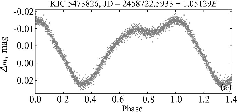
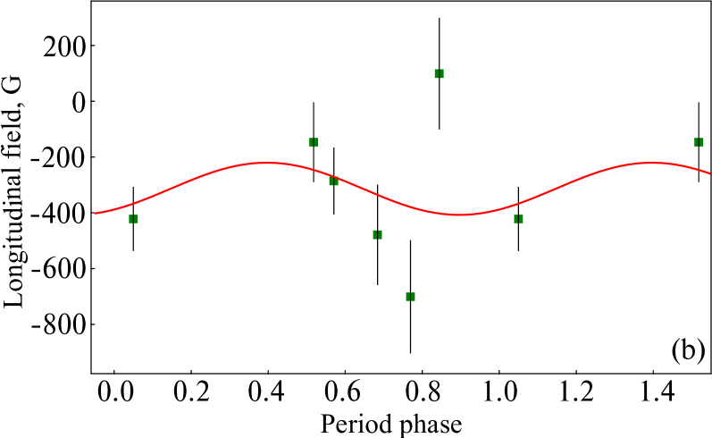
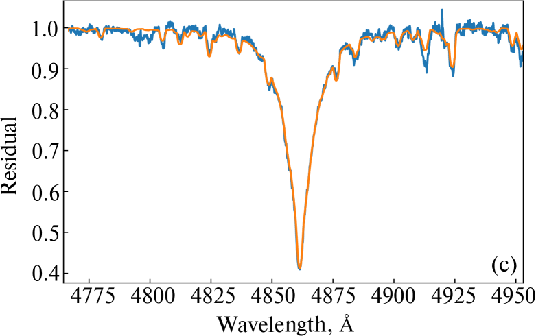
Figure 3: Same as in Fig. 1, for KIC 5473826.

The best matched ephemeris is

$${\rm JD}=2458722.5933+1.05129E.$$

The resulting light curve (Fig. 3a) is characterized by weakly pronounced secondary extrema comparable to the primary maximum. The primary minimum is in the phase $\phi=0.34$, the secondary maximum and minimum are in the phases: $\phi=0.70$ and $\phi=0.80$ respectively. The full amplitude of the brightness variation $\Delta m=0\hbox{$\,.\!\!^{\rm m}$}042$.

Despite the fact that the statistical criterion indicates reliable detection ($\chi^{2}/n=6.62$), the magnetic field is determined with a large error due to wide and non-Gaussian line profiles in the spectrum. The only field measurement with a positive sign is in the region of the secondary minimum of the light curve. Moreover, very close, in the phase of the secondary maximum, there is a negative extremum of the field. The observed data for more reliable approximation of the magnetic curve are not enough. The study of this target will be continued.

When approximating the spectrum (Fig. 3c), the following atmospheric parameters were obtained: $T_{\rm eff}=12\,479$ K, $\log g=3.82$, $v_{e}\sin i=83.39$ km s^-1, and $V_{R}=5.69$ km s^-1.

3.4 KIC 6065699 = HD 188101

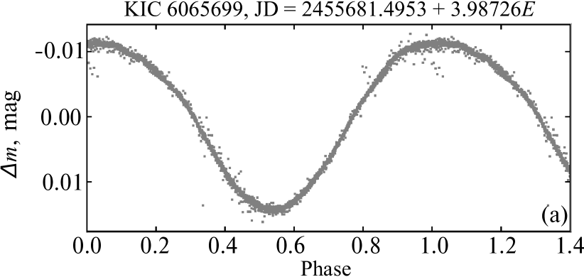
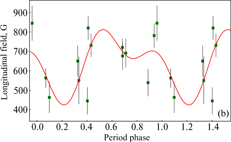
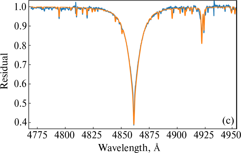
Figure 4: Same as in Fig. 1, for KIC 6065699.

The best ephemeris:

$${\rm JD}=2455681.4953+3.98726E.$$

The light curve is a smooth almost harmonic sine curve with the maximum in the phase $\phi=0.0$ and the minimum in the phase $\phi=0.55$ (Fig. 4a). The total amplitude of the brightness variation $\Delta m=0\hbox{$\,.\!\!^{\rm m}$}022$.

The magnetic fields, on the contrary, show large scatter and are difficult to approximate, despite the large number of measurements that have only positive polarity (see Fig. 4b). These features can be explained by the fact that the positive pole of the dipole is slightly deviated from the rotation axis of the star and directed towards the observer. This explanation is supported by the narrow spectral line profiles which are instrumental actually. According to $\chi^{2}/n=103.75$, the star KIC 6065699 is magnetic.

Based on the spectrum approximation shown in Fig. 4c, the following parameters are obtained: $T_{\rm eff}\!=\!14\,771$ K, $\log g\!=\!3.83$, $v_{e}\sin i=33.40$ km s^-1, $V_{R}=-1.93$ km s^-1, and $[{\rm M/H}]=-0.006$ (see Fig. 4).

When approximating the observed spectrum with a synthetic one, two problems arose.

The first is related to the impossibility of approximating the Si II and Si III lines by a model with one temperature. Good approximation of Si II required a model with the temperature $T_{\rm eff}=15\,200$ K, and for Si III—$T_{\rm eff}=17\,200$ K. Most likely, this difference is caused by the stratification of this element in the atmosphere of the star.

The second problem is the impossibility of approximating the forbidden line He I $\lambda$ 4471. In this case, difficulties arise due to the fact that this line can not be described using the LTE approach, which we used in our work. For correct approximation of this line, it is necessary to calculate a non-LTE model.

3.5 KIC 6278403 = HD 181436

The best ephemeris according to the photometric data:

$${\rm JD}=2458694.6385+1.19114E.$$

The light curve is flat, as can be seen in Fig. 5a, the brightness fading lasts longer than brightening. The maximum phase $\phi=0.0$, the minimum—$\phi=0.6$. Some bend is observed at the fading stage in the region of $\phi=0.25$. The amplitude of the curve $\Delta m=0\hbox{$\,.\!\!^{\rm m}$}008$.

Due to large measurement errors, we can not confirm the reliable detection of a field ($\chi^{2}/n=1.21$). According to our data, it varies weakly and does not exceed several hundred gauss in the absolute magnitude. Measurement errors also do not allow us to confidently carry out the approximation. The maximum of the obtained magnetic curve shown in Fig. 5b is positive and shifted from the photometric minimum.

The best fit between the observed and synthetic spectra is achieved with the parameters: $T_{\rm eff}=11\,261$ K, $\log g=4.12$, $v_{e}\sin i=46.5$ km s^-1, and $V_{R}=-12.1$ km s^-1.

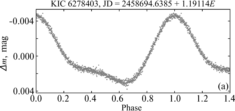
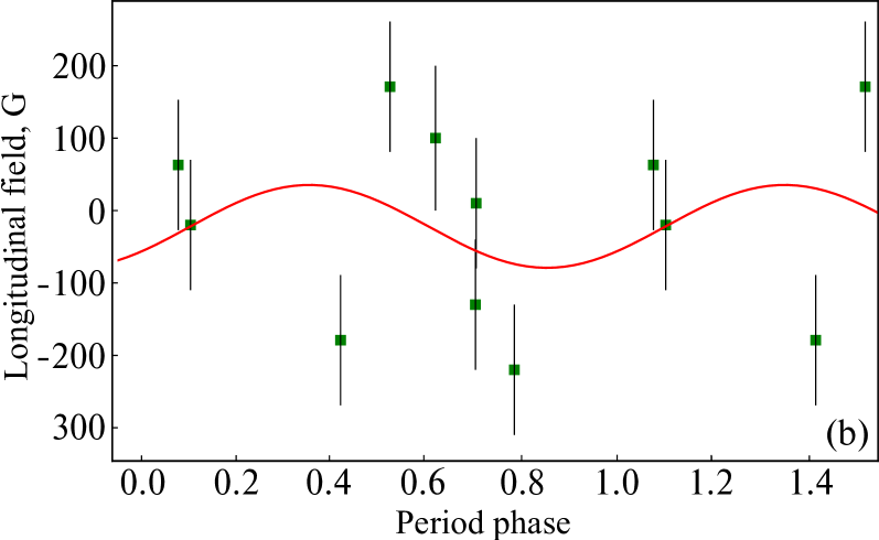
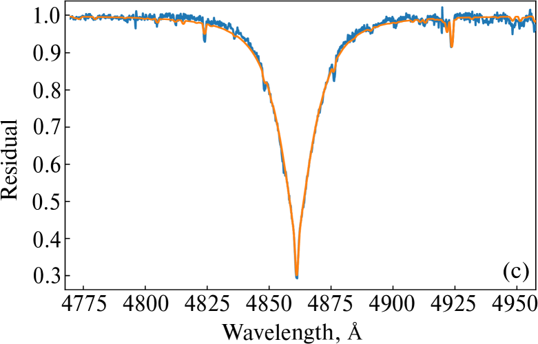
Figure 5: Same as in Fig. 1, for KIC 6278403.

3.6 KIC 6864569 = BD+42^∘3356

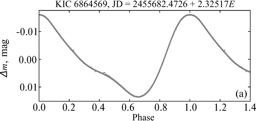
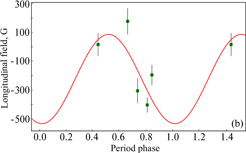
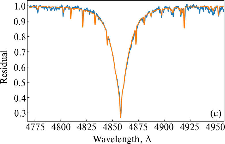
Figure 6: Same as in Fig. 1, for KIC 6864569.

The best ephemeris:

$${\rm JD}=2455682.4726+2.32517E.$$

In shape, the light curve of KIC 6864569 (see Fig. 6a) is remarkably similar to the light curve of KIC 6278403, but the amplitude and period are different. For KIC 6864569, the amplitude $\Delta m=0\hbox{$\,.\!\!^{\rm m}$}03$, and the period of brightness variability $P=2\hbox{$\,.\!\!^{\rm d}$}32517$ which is about twice as much as that for KIC 6278403.

As well as for KIC 6278403, the magnetic field strength of KIC 6864569 does not exceed several hundred gauss and varies slightly with rotation (Fig. 6b). A small number of observation points does not allow us to confidently characterize the magnetic curve. However, the obtained criterion $\chi^{2}/n=16.45$ supports the reliable field detection.

Approximation of the observed spectrum of the star (Fig. 6c) gives the following parameters: $T_{\rm eff}\!=\!10\,612$ K, $\log g\!=\!4.03$, $v_{e}\sin i\!=\!37.02$ km s^-1, and $V_{R}=-17.30$ km s^-1 .

3.7 KIC 8161798 = BD +43 3223

The best ephemeris:

$${\rm JD}=2455680.9554+2.20298E.$$

Figure 7a shows the phase-convolved light curve of KIC 8161798. It is a distinct double wave with primary and secondary minima almost coinciding in magnitude. The primary maximum is followed by the first minimum in the phase $\phi=0.25$, then, the secondary maximum in the phase $\phi=0.5$ followed by another minimum in the phase $\phi=$0.73. The brightness amplitude is relatively high: $\Delta m=0\hbox{$\,.\!\!^{\rm m}$}124$.

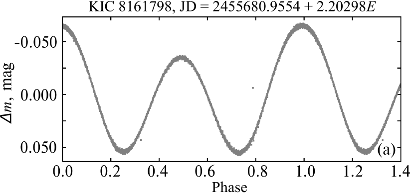
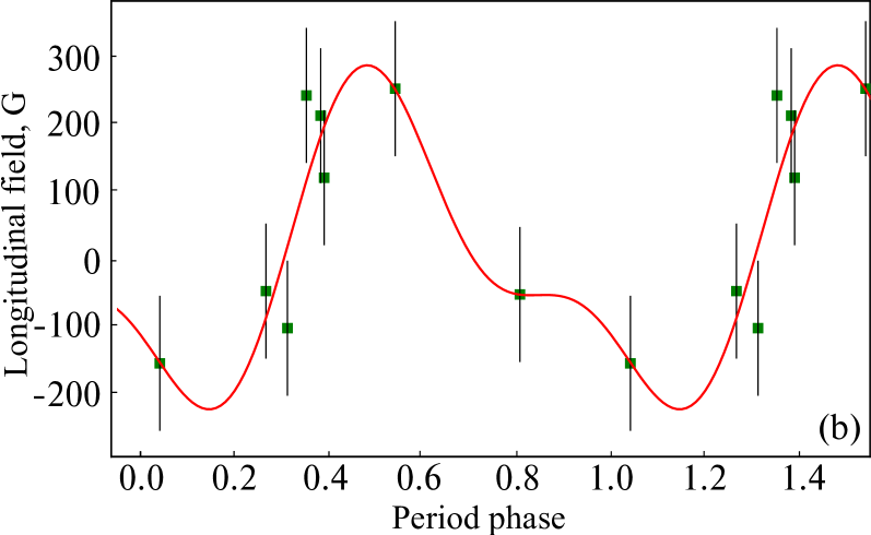
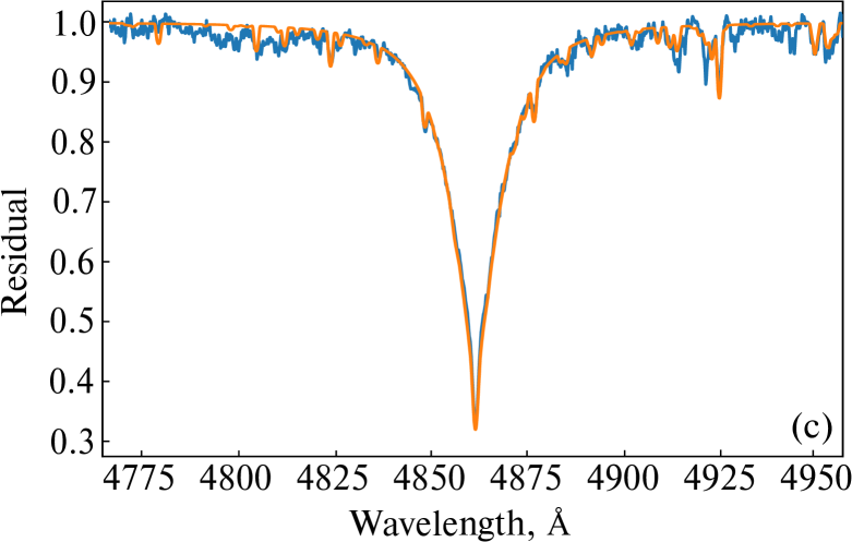
Figure 7: Same as in Fig. 1, for KIC 8161798.

The criterion $\chi^{2}/n=2.75$; the magnetic field is not reliably detected, but its variability is observed. The positive maximum of the magnetic field corresponds in phase to the secondary brightness maximum, the negative maximum is slightly shifted relative to the first brightness minimum.

The parameters obtained on the basis of the spectrum approximation: $T_{\rm eff}=11\,664$ K, $\log g=4.00$, $v_{e}\sin i=49.37$ km s^-1, and $V_{R}=-37.3$ km s^-1 (see Fig. 7c).

3.8 KIC 8324268 = HD 189160

The best ephemeris according to the TESS satellite:

$${\rm JD}=2458734.7007+2.00912E.$$

Figure 8 presents the resulting light curve of KIC 8324268, the phase curve of the magnetic field, and the H${\beta}$-line modeling result in the spectrum of the object. The shape of the light curve is a single wave and almost a harmonic sine curve. Note its similarity with the light curve of KIC 6065699. The brightening interval is slightly longer than the fading interval. The brightness maximum and minimum correspond to the phases: $\phi=0.0$ and $\phi=0.45$. The brightness amplitude $\Delta m=0\hbox{$\,.\!\!^{\rm m}$}026$.

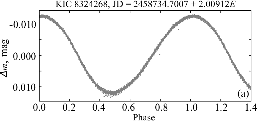
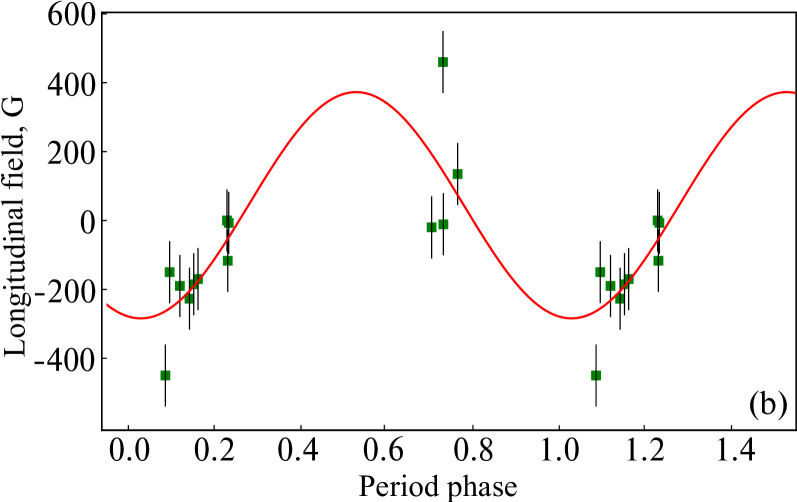
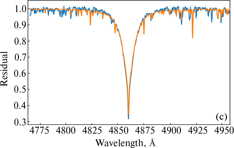
Figure 8: Same as in Fig. 1, for KIC 8324268.

Magnetic field measurements show large scatter (see Fig. 8b), which makes it difficult to approximate by a single wave, but the criterion $\chi^{2}/n=5.88$ indicates its reliable detection.

The spectrum approximation (Fig. 8c) gives the following parameters: $T_{\rm eff}=12\,996$ K, $\log g=3.85$, $v_{e}\sin i=26.0$ km s^-1, and $V_{R}=-17.5$ km s^-1.

3.9 KIC 10324412 = HD 176436

When analyzing the time series from the TESS satellite, the ephemeris was obtained:

$$JD=2455680.7844+1.73150E.$$

The light curve of the object is a double wave with a primary and secondary maximum near the phases $\phi=0.0$ and $\phi=0.6$ respectively. The brightness minimum is near the phase $\phi=0.3$, the brightness variation amplitude $\Delta m=0\hbox{$\,.\!\!^{\rm m}$}03$. (see Fig. 9a).

The magnetic field is very weak, almost at the detection limit showing a single sinusoid with the minimum near the primary maximum of the light curve and with the maximum near the secondary (Fig. 9b). The estimate $\chi^{2}/n=0.89$ does not allow one to assert the reliable detection of a magnetic field.

The parameters determined during the spectrum approximation: $T_{\rm eff}=10\,142$ K, $\log g=3.99$, $v_{e}\sin i=77.73$ km s^-1, $V_{R}=1.39$ km s^-1, and ${\rm[{\rm M/H}]}=0.544$. The observed and synthetic spectra are shown in Fig. 9c.

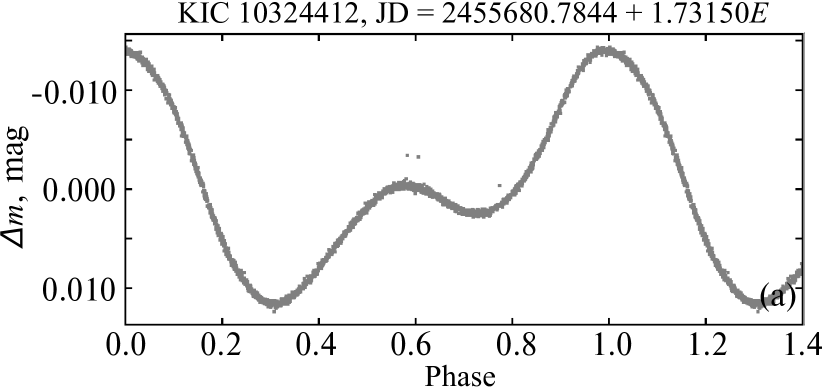
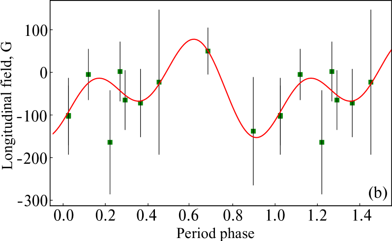
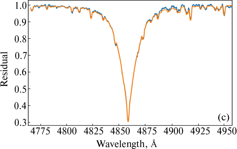
Figure 9: Same as in Fig. 1, for KIC 10324412.

3.10 KIC 11560273 = HD 184007

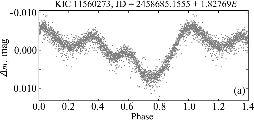
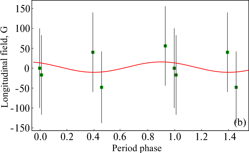
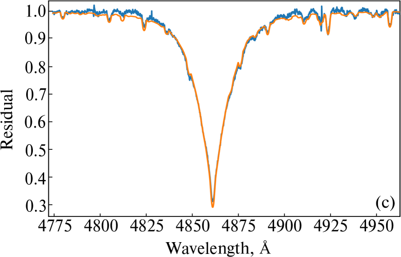
Figure 10: Same as in Fig. 1, for KIC 11560273.

The best ephemeris:

$${\rm JD}=2458685.1555+1.82769E.$$

Figure 10a shows the phased light curve of the object. Its shape is another example of the previously noted diversity of light curves of mCP star candidates. The total amplitude of the brightness variation $\Delta m=0\hbox{$\,.\!\!^{\rm m}$}02$.

Measurements of the longitudinal magnetic field strength are burdened with large errors (Fig. 10b). The estimate $\chi^{2}/n=0.16$ indicates that no magnetic field is detected.

Figure 10c presents the observed spectrum of the object and the result of its synthetic approximation with the following model parameters: $T_{\rm eff}=9\,744$ K, $\log g=3.77$, $v_{e}\sin i=73.8$ km s^-1, and $V_{R}=-15.5$ km s^-1.

4 CONCLUSION

We present the first results of studying the variability of a part of the mCP star candidate sample that we have compiled using the analysis of the Kepler satellite photometric data. The proposed candidate selection method demonstrates its effectiveness: the spectra of all the stars in the sample contain peculiar lines which has been previously demonstrated in the paper by Hümmerich et al. (2018), observations for which have been obtained with the Zeiss-1000 SAO RAS telescope. The magnetic fields are reliably detected in six stars out of the ten objects selected for monitoring: KIC 4180396, KIC 5264818, KIC 5473826, KIC 6065699, KIC 6864569, and KIC 8324268. For the remaining four objects, the field is detected at the level of instrumental measurement errors during observations with the MSS at the SAO RAS BTA.

Curiously, the shapes of the light curves of the objects show extraordinary variety. Most likely, this can be explained by the spotted surface structures characteristic of CP stars. For the future, there are plans to study the effect of spots of individual chemical elements on the shape of the photometric light curves.

At the present stage, it is difficult to talk about regularities in correlation between the behavior of the magnetic field and photometric curves. Only for three objects (KIC 4180396, KIC 5264818, and KIC 8161798) positive or negative extrema of the magnetic curves correspond to the photometric extrema (primary or secondary). To eliminate the random factor, a large sample of objects is needed.

Spectropolarimetric monitoring of the photometric candidate sample will be continued.

FUNDING

The observation part of the study and data reduction (IY) were carried out with the financial support of the RFBR within the framework of the scientific project No. 19-32-60007.

Analyzing and building the magnetic field phase curves, determination of physical parameters (EAS, IIR, and AVM) were carried out with partial financial support from the Russian Science Foundation (RSF) No. 21-12-00147.

CONFLICT OF INTEREST

The authors declare no conflict of interest regarding the publication of this paper.

References

- Chountonov (2016) G. A. Chountonov, Astrophysical Bulletin 71 (4), 489 (2016).
- Bagnulo et al. (2002) S. Bagnulo, T. Szeifert, G. A. Wade, et al., Astronomy and Astrophysics, 389, 191 (2002).
- David-Uraz et al. (2019) A. David-Uraz, C. Neiner, J. Sikora, et al., Monthly Notices Royal Astron. Soc. 487 (1), 304 (2019).
- Deutsch (1970) A. J. Deutsch, Astrophys. J. 159, 985 (1970).
- Dukes and Adelman (2018) J. R. Dukes Jr. and S. J. Adelman, Publ. Astron. Soc. Pacific 130 (986), 044202 (2018).
- Hümmerich et al. (2018) S. Hümmerich, Z. Mikulášek, E. Paunzen, et al., Astron. and Astrophys. 619, id. A98 (2018).
- Kholtygin et al. (2019) A. F. Kholtygin, O. A. Tsiopa, E. I. Makarenko, and I. M. Tumanova, Astrophysical Bulletin 74 (3), 293 (2019).
- Krtička et al. (2012) J. Krtička, Z. Mikulášek, T. Lüftinger, et al., Astron. and Astrophys. 537, id. A14 (2012).
- Kudryavtsev (2000) D. O. Kudryavtsev, Baltic Astronomy 9, 649 (2000).
- Kudryavtsev et al. (2006) D. O. Kudryavtsev, I. I. Romanyuk, V. G. Elkin, and E. Paunzen, Monthly Notices Royal Astron. Soc. 372, 4, 1804-1828 (2006).
- Lafler and Kinman (1965) J. Lafler and T. D. Kinman, Astrophys. J. Suppl. 11, 216 (1965).
- Landstreet and Bagnulo (2019) J. D. Landstreet and S. Bagnulo, Astron. and Astrophys. 628, id. A1 (2019).
- Maitzen (1984) H. M. Maitzen, Astron. and Astrophys. 138, 493 (1984).
- Mathys and Manfroid (1985) G. Mathys and J. Manfroid, Astron. and Astrophys. Suppl. 60, 17 (1985).
- Mikulášek et al. (2018) Z. Mikulášek, J. Krtička, E. Paunzen, et al., Contrib. Astron. Obs. Skalnate Pleso 48 (1), 203 (2018).
- Mikulášek et al. (2019) Z. Mikulášek, E. Paunzen, S. Hümmerich, et al., ASP Conf. Ser. 518, 117 (2019).
- Panchuk et al. (2014) V. E. Panchuk, G. A. Chuntonov, and I. D. Naidenov, Astrophysical Bulletin 69 (3), 339 (2014).
- Paunzen et al. (2005) E. Paunzen, C. Stütz, and H. M. Maitzen, Astron. and Astrophys. 441, 631 (2005).
- Piskunov and Valenti (2017) N. E. Piskunov and J. A. Valenti, Astron. and Astrophys. 597, id. A16 (2017).
- Piskunov et al. (1995) N. E. Piskunov, F. Kupka, T. A. Ryabchikova, et al., ASP Conf. Ser. 81, 610 (1995).
- Preston (1974) G. W. Preston, Annual Rev. Astron. Astrophys. 12, 257 (1974).
- Ricker et al. (2015) G. R. Ricker, J. N. Winn, R. Vanderspek, et al., J. Astron. Telescopes, Instruments, and Systems 1, id. 014003 (2015).
- Semenko et al. (2022) E. Semenko, I. Romanyuk, I. Yakunin, D. Kudryavtsev, A. Moiseeva A., Monthly Notices Royal Astron. Soc. 515, 998 (2022).
- Romanyuk et al. (2019) I. I. Romanyuk, E. A. Semenko, A. V. Moiseeva, et al. Astrophysical Bulletin 74 (1), 55 (2019).
- Schöller et al. (2017) M. Schöller, S. Hubrig, L. Fossati, et al., Astron. and Astrophys. 599, id. A66 (2017).
- Shulyak et al. (2004) D. Shulyak, V. Tsymbal, T. Ryabchikova, et al., Astron. and Astrophys. 428, 993 (2004).
- Žižňovský (1994) J. Žižňovský, in Proc. Intern. Conf. on Chemically peculiar and magnetic stars, Tatranska Lomnica, Slovak Republic, 1993, Ed. by J. Zverko and J. Žižňovský (Tatranska Lomnica, 1994), p. 155.
- Wade et al. (2016) G. A. Wade, C. Neiner, E. Alecian, et al., Monthly Notices Royal Astron. Soc. 456 (1), 2 (2016).