Efficient vectors in priority setting methodology
Abstract
The Analytic Hierarchy Process (AHP) is a much discussed method in ranking business alternatives based on empirical and judgemental information. We focus here upon the key component of deducing efficient vectors for a reciprocal matrix of pair-wise comparisons. It is not known how to produce all efficient vectors. It has been shown that the entry-wise geometric mean of all columns is efficient for any reciprocal matrix. Here, by combining some new basic observations with some known theory, we 1) give a method for inductively generating large collections of efficient vectors, and 2) show that the entry-wise geometric mean of any collection of distinct columns of a reciprocal matrix is efficient. Based on numerical simulations, there seems to be no clear advantage over either the geometric mean of all columns or the right Perron eigenvector of a reciprocal matrix.
Keywords: Decision analysis, consistent matrix, efficient vector, geometric mean, reciprocal matrix.
MSC2020: 90B50, 91B06, 15A60, 05C20
1 Introduction
A method used in decision-making and frequently discussed in the literature is the Analytic Hierarchy Process (AHP), suggested by Saaty [31, 32]. Several works since then have developed and discussed many aspects of the method. See the surveys [11, 25, 34]. A key element of the method is the notion of pair-wise comparison (PC) matrix. An -by- positive matrix is called a PC matrix if, for all
Each diagonal entry of a PC matrix is We refer to the set of all such matrices as . Often, we refer to these matrices as reciprocal matrices, as do other authors.
The entry of a reciprocal matrix is viewed as a pair-wise ratio comparison between alternatives and and the intent is to deduce an ordering of the alternatives from it. If the reciprocal matrix is consistent (transitive): for all triples there is a unique natural cardinal ordering, given by the relative magnitudes of the entries in any column. However, in human judgements consistency is unlikely. Inconsistency can also be an inherent feature of objective datasets [8, 10, 14, 29, 30]. Then, there will be many vectors that might be deduced from a reciprocal matrix . Let be a positive -vector and the transpose of its component-wise inverse. We may try to approximate by the consistent matrix i.e., we wish to choose so that is small in some sense. We say that is efficient for if, for any other positive vector and corresponding consistent matrix the entry-wise inequality implies that and are proportional. (It follows from Lemma 5 that we give later that this definition is equivalent to that of other authors for the notion of efficiency [6, 9]). Clearly, a consistent approximation to a reciprocal matrix should be based upon a vector efficient for If is not itself consistent, the set of efficient vectors for will include many vectors not proportional to each other. This set is, however, at least connected [6], but, in general, it is difficult to determine the entire set For simplicity, we projectively view proportional efficient vectors as the same, as they produce the same consistent matrix. Several methods to study when a vector is efficient were developed and algorithms to improve an inefficient vector have been provided (see [3, 6, 7, 9, 20, 22] and the references therein).
Despite some criticism [18, 19, 26, 33], one of the most used methods to approximate a reciprocal matrix by a consistent matrix is the one proposed by Saaty [31, 32], in which the consistent matrix is based upon the right Perron eigenvector of , a positive eigenvector associated with the spectral radius of [24]. The efficiency of the Perron eigenvector for certain classes of reciprocal matrices has been shown [1, 2, 20], though examples of reciprocal matrices for which this vector is inefficient are also known [4, 6, 7]. Another method to approximate by a consistent matrix is based upon the geometric mean of all columns of which is known to be an efficient vector for [6]. Many other proposals for approximating by a consistent matrix have been made in the literature (for comparisons of different methods see, for example, [4, 11, 17, 21, 23, 27]).
Before summarizing what we do here, we mention some more notation and terminology. The Hadamard (or entry-wise) product of two vectors (of the same size) or matrices (of the same dimension) is denoted by For example, if then , and, similarly, the -by- consistent matrices are closed under the Hadamard product. We use superscripts in parentheses to denote an exponent applied to all entries of a vector or a matrix. For example
is the (Hadamard) geometric mean of positive vectors of the same size. This column geometric mean is what is called the row geometric mean for instance in [6].
For an -by- matrix we partition by columns as The principal submatrix determined by deleting (by retaining) the rows and columns indexed by a subset is denoted by we abbreviate as Note that if is reciprocal (consistent) then so is
In Section 2 we give some (mostly known) background that we will use and make some related observations. In particular, we present the relationship between efficiency and strong connectivity of a certain digraph and state the efficiency of the Hadamard geometric mean of all the columns of a reciprocal matrix. In Section 3 we give some (mostly new) additional background that will also be helpful. In Section 4 we show explicitly how to extend efficient vectors for to efficient vectors for the reciprocal matrix This leads to an algorithm initiated by any , to produce a subset of This subset may not be all of as truncation of an efficient vector for may not give one for the corresponding principal submatrix. And we may get different subsets by starting with different In Section 5 we study the relationship between efficient vectors for a reciprocal matrix and its columns. As mentioned, any column of a consistent matrix generates that consistent matrix and, so, is efficient for it. Similarly, any column of a reciprocal matrix is efficient for it (Lemma 10), as is the geometric mean of any subset of the columns (Theorem 12). In Section 6, we study numerically, using different measures, the performance of these efficient vectors in approximating by a consistent matrix and compare them, from this point of view, with the Perron eigenvector (in cases in which it is efficient). It will be clear that the geometric mean of all columns can be significantly outperformed by the geometric mean of other collections of columns. We also show by example that is not closed under geometric mean (Section 5). Finally, in Section 7 we give some conclusions.
2 Technical Background
We start with some known results that are relevant for this work. First, it is important to know how changes when is subjected to either a positive diagonal similarity or a permutation similarity, or both (a monomial similarity).
Lemma 1
Next we define a directed graph (digraph) associated with a matrix and a positive -vector which is helpful in studying the efficiency of for For , we denote by the directed graph (digraph) whose vertex set is and whose directed edge set is
In [6] the authors proved that the efficiency of can be determined from .
Theorem 2
[6] Let . A positive -vector is efficient for if and only if is a strongly connected digraph, that is, for all pairs of vertices with there is a directed path from to in .
Recall [24] that is strongly connected if and only if is positive. Here is the identity matrix of order and is the adjacency matrix of that is, if is an edge in and otherwise.
In [6], it was shown that the geometric mean of all the columns of a reciprocal matrix is an efficient vector for . This result comes from the fact that the geometric mean minimizes the logarithmic least squares objective function (see also [12]).
Theorem 3
[6]If then
In [13], all the efficient vectors for a simple perturbed consistent matrix, that is, a reciprocal matrix obtained from a consistent one by perturbing one entry above the main diagonal and the corresponding reciprocal entry, were described. Let with be the matrix in with all entries equal to except those in positions and which are and respectively. For any simple perturbed consistent matrix there is a positive diagonal matrix and a permutation matrix such that
for some Taking into account Lemma 1, an -vector is efficient for if and only if is efficient for For this reason, we focused on the description of the efficient vectors for as the efficient vectors for a general simple perturbed consistent matrix can be obtained from them using Lemma 1.
Theorem 4
3 Additional facts on efficiency
From the following result we may conclude that the definition of efficient vector given in Section 1 is equivalent to the one in [6, 9].
Here and throughout, if and is a positive -vector, we denote
By we mean the entry-wise absolute value of
Lemma 5
Let and be positive -vectors. Then, if and only if and are proportional.
Proof. The ”if” claim is trivial. Next we show the ”only if” claim. Let and Let with Suppose that
| (1) |
If
then (1) implies If
then also
implying, from (1),
So
Condition for all implies and proportional.
We close this section with a topological property of .
Theorem 6
For any is a closed set.
Proof. We verify this by showing that the inefficient vectors, in the complementary of form an open set, by appealing to Theorem 2. Suppose that then the graph is not strongly connected. Let be a sufficiently small perturbation of (i.e. lies in an open ball about whose radius is positive, but as small as we like). Then, if is not an edge of then it is not an edge of Then has no more edges (under inclusion) than Since the latter was not strongly connected, the former also is not, so that
We also note that, if and the matrix has no off-diagonal entries, then for any sufficiently small perturbation of and for any sufficiently small reciprocal perturbation of
4 Inductive construction of efficient vectors
Suppose that and that Then is strongly connected. May be extended to an efficient vector for and, if so, how? For a positive scalar the vector if and only if is strongly connected. But, since the subgraph induced by vertices of is and the latter is strongly connected, is strongly connected if and only if there are edges from vertex to vertices in and also edges from the latter to (see Proposition 3 in [13]). Since the vector of the first entries of the last column of is less the vector of the first entries of (the last column of , there are such edges if and only if this difference vector has a entry or both positive and negative entries. This means that among there are both nonnegative and nonpositive numbers. We restate this as
Theorem 7
For and the vector
if and only if the scalar satisfies
Of course, the above interval is nonempty. This leads to a natural algorithm to construct a large subset of for
Choose the upper left principal submatrix of It is consistent and, up to a factor of scale, has only one efficient vector Now extend this vector, in all possible ways, to an efficient vector for according to Theorem 7. This gives the set Now, continue extending each vector in to an element of in the same way, and so on. This terminates in a subset
We make two important observations. First, we may instead start with some other -by- principal submatrix and proceed similarly, either by inserting the new entry of the next efficient vector in the appropriate position, or by placing in the upper left -by- submatrix, via permutation similarity, and proceeding in exactly the same way. We note that starting in two different positions may produce different terminal sets (Example 8), and the union of all possible terminal sets is contained in
Second, may be a proper subset of as truncation of a vector (deletion of an entry) from an efficient vector for may not give an efficient vector for the corresponding principal submatrix (see Example 8).
Example 8
Let
The efficient vectors for are proportional to
By Theorem 7, the vectors of the form
with
are efficient for (and, of course, all positive vectors proportional to them).
The efficient vectors for are proportional to
By Theorem 7, the vectors of the form
with
are efficient for
The efficient vectors for are proportional to
By Theorem 7, the vectors of the form
with
are efficient for
Note that, by Theorem 4,
For example, the vector is efficient for though it does not belong to the set of vectors determined above, as no vector obtained from it by deleting one entry is efficient for the corresponding -by- principal submatrix.
There are cases in which we know all the efficient vectors for a larger submatrix and then we can start our building process with this submatrix. In fact, taking into account Theorem 4, all efficient vectors for a -by- reciprocal matrix are known, as such matrix is a simple perturbed consistent matrix. Thus, it is always possible to start the process from a -by- principal submatrix.
Example 9
Consider the matrix
| (2) |
By Theorem 4, the efficient vectors for are the vectors of the form
with By Theorem 7, the vectors of the form
with
are efficient for Again by Theorem 7, the vectors of the form
with
are efficient for For instance, the vectors
with are efficient for Moreover, these are the only efficient vectors with the given first four entries.
We observe that, if is a (inconsistent) simple perturbed consistent matrix, then has a principal -by- (inconsistent) simple perturbed consistent submatrix If we start the inductive construction of efficient vectors for with the submatrix for which is known by Lemma 1 and Theorem 4, then we obtain This fact follows from Corollary 9 in [13], taking into account that, by Lemma 1, and Remark 4.6 in [22], we may focus on for some
Similarly, if is a double perturbed consistent matrix (that is, is obtained from a consistent matrix by modifying two entries above the diagonal and the corresponding reciprocal entries), in which no two perturbed entries lie in the same row and column, then has a principal -by- double perturbed consistent submatrix of the same type and, by Theorem 4.2 in [22] and Lemma 1, is known. By Corollary 4.5 in [22], if we start the inductive construction of efficient vectors with then again we obtain
5 Columns of a reciprocal matrix
Previously, it has been noted (Theorem 3) that the Hadamard geometric mean of all columns of is efficient for . Interestingly, each individual column of is efficient.
Lemma 10
Let Then any column of lies in
Proof. Let be the -th column of Then the -th column of has entries . Hence, has an undirected star on vertices as an induced subgraph and is, therefore, strongly connected, verifying that is efficient, by Theorem 2.
Further, the geometric mean of any subset of the columns of a reciprocal matrix also lies in To prove this result, we use the following lemma.
Lemma 11
Let be a positive diagonal matrix and If is the geometric mean of columns of then is a positive multiple of the geometric mean of the corresponding columns of
Proof. By a possible permutation similarity and taking into account Lemma 1, suppose, without loss of generality, that is the geometric mean of the first columns of . (Note that, if is the geometric mean of a reciprocal matrix then is the geometric mean of for a permutation matrix ) The -th entry of is . On the other hand, the -th entry of the geometric mean of the first columns of is Thus, the quotient of the -th entries of and is which does not depend on implying the claim.
Theorem 12
Let Then the geometric mean of any collection of distinct columns of lies in
Proof. Let We show that the geometric mean of distinct columns of is efficient for The proof is by induction on . For the result is straightforward. Suppose that If or the result follows from Lemma 10 or Theorem 3, respectively. Suppose that By Lemmas 1 and 11, we may and do assume that the columns of are the first ones, and the entries in the last column and in the last row of are all equal to , that is,
where is the -vector with all entries equal to and . Let be the first columns of so that, for
We have
in which is the geometric mean of columns By the induction hypothesis, is efficient for so that, by Theorem 2, is strongly connected. Thus, is strongly connected if and only if there are edges from vertex to vertices in and also vertices from the latter to (see the observation before Theorem 7). Then, is strongly connected if and only if is neither strictly positive nor negative. The product of the first entries of is , where is the product of the entries of Since this matrix is reciprocal, then Thus, the vector formed by the first entries of is neither strictly greater than nor strictly less than , implying that is strongly connected.
We observe that we have (nonempty) distinct subsets of columns of (not necessarily corresponding to different geometric means).
The sets of efficient vectors for matrices in (any -by- reciprocal matrix is consistent) and in (any -by- reciprocal matrix is a simple perturbed consistent matrix) are closed under geometric means. In the latter case, this follows from Lemma 1 and the facts that a matrix in is monomial similar to for some , and, by Theorem 4, the set of efficient vectors for is closed under geometric mean. However, the set of efficient vectors for matrices in with may not be closed under geometric mean, as the next example illustrates.
Example 13
Let be the matrix in (2). Let
the -by- principal submatrix of obtained by deleting the -th row and column. Taking into account Example 9, the vectors
are efficient for However the vector is not efficient for as the first three entries of the last column of are positive and, therefore, is not strongly connected.
6 Numerical experiments
We next give numerical examples in which we compare the geometric means of the vectors in different proper subsets of columns of a reciprocal matrix with the geometric mean of all columns of denoted here by a vector proposed by several authors to obtain a consistent matrix approximating , as this method has a strong axiomatic background [5, 15, 16, 21, 28]. Recall from Section 5 that all these vectors are efficient for We take the sum of all entries of as a measure of effectiveness of as well as the Frobenius norm of Recall that, for an -by- matrix we have
Other measures (norms) are possible. For comparison, we also consider the case in which is the Perron eigenvector of denoted by , as it is one of the most used vectors to estimate a consistent matrix close to . Our experiments were done using the software Octave version 6.1.0.
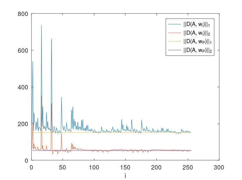
Example 14
Consider the matrix
There are distinct subsets of the set of columns of We identify each subset with a sequence of five numbers, in which a in position means that the -th column of belongs to the subset, while a means that it does not belong to the subset. The sequences are in increasing (numerical) order and by we denote the subset of columns associated with the -th sequence. Note that is the set of all columns of By we denote the geometric mean of the vectors in
In Table 1 we give the norms and In Table 2 we emphasize the results obtained for the geometric mean of all columns, for the vectors that produce the smallest and the largest values of and and also consider the case of the Perron eigenvector of (which is efficient). Note that
It can be observed that, according to the considered measures, there are proper subsets of columns that produce better results than those for the Perron eigenvector and for the set of all columns.
We summarize our results in Figure 1, in which we give a graphic with a comparison of all the results obtained. In the axis we have the index of each subset of columns. In the axis we have the values of and for the different vectors A line jointing the values of each of these norms for the different subsets of columns is plotted. A horizontal line corresponding to each of the considered norms for the Perron eigenvector also appears.
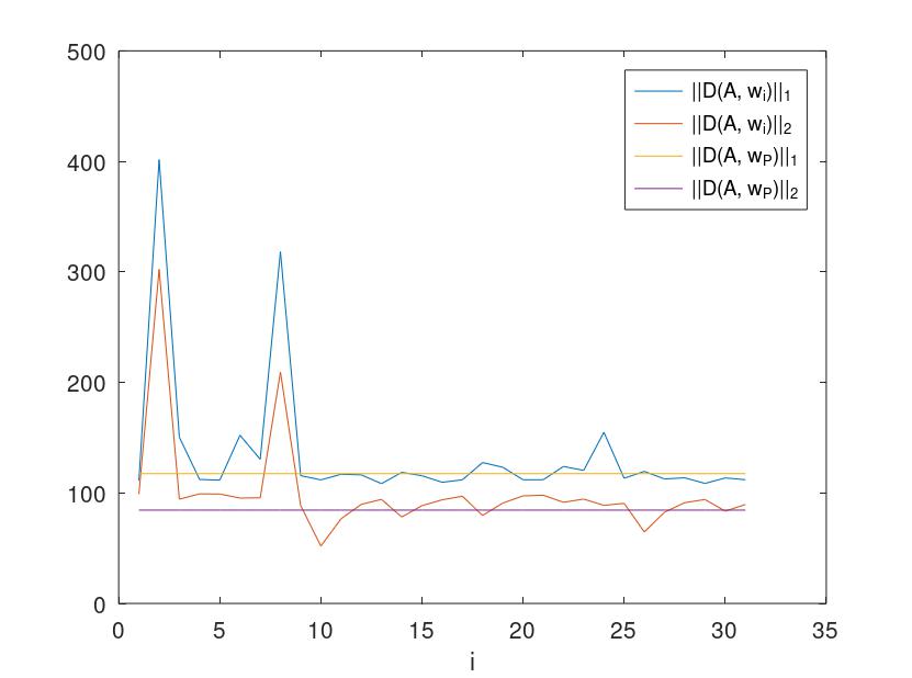
Example 15
Consider the matrix
Table 3 and Figure 2 are the analogs of Table 2 and Figure 1 for the -by- reciprocal matrix considered here. Note that in this case we have different subsets of the set of columns of Again, a proper subset of the columns produces better results than either all columns or the Perron vector (which is efficient for ). Note that
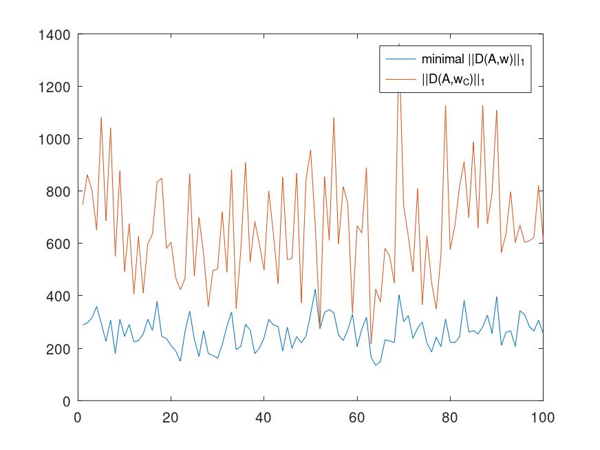
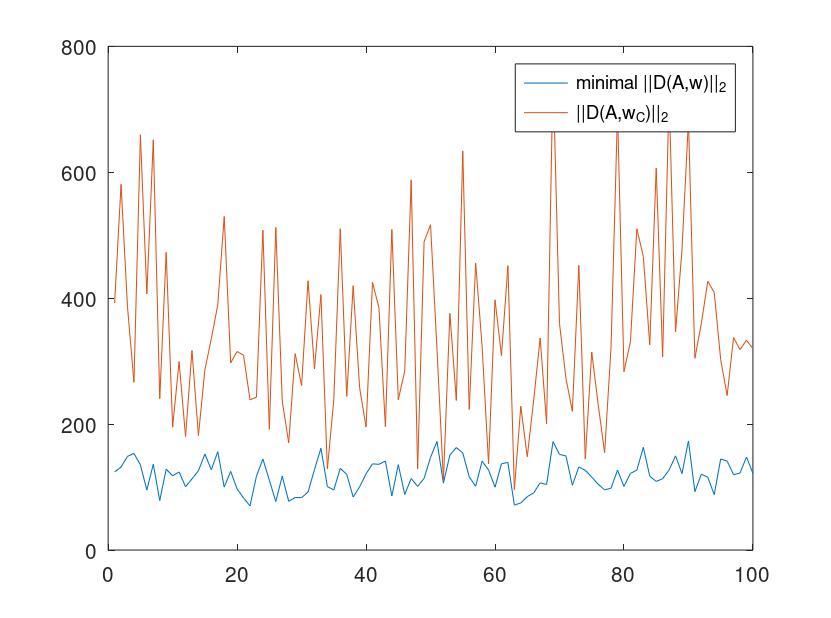
Experiment 16
In this example we generated reciprocal matrices in which the entries in the upper triangular part are random real numbers in the interval and compare, in terms of the 1-norm (Figure 3) and the Frobenius norm (Figure 4) of the cases in which is the geometric mean of all columns of and is the vector that produces the smallest norm among all geometric means of the subsets of the columns of Again, it can be verified that, in general, a proper subset of columns produce better results.
In our previous examples we have emphasized that the minimum -norm and the minimum Frobenius norm of when runs over the geometric means of the sets of columns of a reciprocal matrix is, in general, not attained by the geometric mean of all columns of However, if we consider a large set of random reciprocal matrices , we can see that the sum, for all ’s, of some normalization of performs well when compared to the corresponding sums for other sets of columns, even when with running over the geometric means of the subsets of columns of is not attained by for most ’s.
Experiment 17
We consider reciprocal matrices , by generating matrices with random real entries in the interval and letting where denotes the entry-wise inverse of and the Hadamard product. For each we determine
in which is the geometric mean of subset of the columns of (We identify the subsets with indices of columns, as introduced in Example 14.) In Table 4 we display the values of For each we also display the number of ’s for which , when runs over all the geometric means of the subsets of columns of , is attained by the subset .
We finally give an example illustrating that, close to consistency, all subsets of columns perform about the same, as expected.
7 Conclusions
In the context of the Analytic Hierarchic Process, pairwise comparison matrices (PC matrices), also called reciprocal matrices, appear to rank different alternatives. In practice, the obtained reciprocal matrices are usually inconsistent and a good consistent matrix approximating the reciprocal matrix should be obtained. A consistent matrix is uniquely determined by a positive vector (the vector of priorities or weights). Many methods have been proposed in the literature to obtain the vectors from which a consistent matrix approximating a given reciprocal matrix is constructed. Some of the most used methods consist on the choice of the Perron eigenvector of the reciprocal matrix or on the Hadamard geometric mean of all its columns. An important property that should be satisfied by the vectors on which such a consistent matrix is based is efficiency. It is known that the Hadamard geometric mean of all the columns of a reciprocal matrix is efficient, though the Perron eigenvector not always satisfies this property.
Here we give an algorithm to construct efficient vectors for a reciprocal matrix from efficient vectors for principal submatrices of We also show that the geometric mean of the vectors in any nonempty subset of the columns of is efficient for We give an example that the geometric mean of two efficient vectors need not be efficient. It leaves the question of when the Hadamard geometric mean of two efficient vectors is efficient.
We give numerical examples comparing the geometric means obtained from proper subsets of the columns of with the geometric mean of all the columns of We conclude that the geometric mean of some proper subsets of columns may produce better results, also when compared with the Perron eigenvector, which we include for completeness. So, according to our results, there is no evidence that the geometric mean of all columns has a universal advantage over the geometric means of other sets of columns, specially when the level of inconsistency is significant.
Declaration All authors declare that they have no conflicts of interest.
References
- [1] K. Ábele-Nagy, S. Bozóki, Efficiency analysis of simple perturbed pairwise comparison matrices, Fundamenta Informaticae 144 (2016), 279-289.
- [2] K. Ábele-Nagy, S. Bozóki, Ö. Rebák, Efficiency analysis of double perturbed pairwise comparison matrices, Journal of the Operational Research Society 69 (2018), 707-713.
- [3] M. Anholcer, J. Fülöp, Deriving priorites from inconsistent PCM using the network algorithms, Annals of Operations Research 274 (2019), 57-74.
- [4] G. Bajwa, E. U. Choo, W. C. Wedley, Effectiveness analysis of deriving priority vectors from reciprocal pairwise comparison matrices, Asia-Pacific Journal of Operational Research, 25(3) (2008), 279–299.
- [5] J. Barzilai, Deriving weights from pairwise comparison matrices, Journal of the Operational Research Society 48(12) (1997), 1226-1232.
- [6] R. Blanquero, E. Carrizosa, E. Conde, Inferring efficient weights from pairwise comparison matrices, Mathematical Methods of Operations Research 64 (2006), 271-284.
- [7] S. Bozóki, Inefficient weights from pairwise comparison matrices with arbitrarily small inconsistency, Optimization 63, 1893-1901 (2014).
- [8] S. Bozóki, L. Csató, J. Temesi, An application of incomplete pairwise comparison matrices for ranking top tennis players, European Journal of Operational Research 248(1) (2016), 211–218.
- [9] S. Bozóki, J. Fülöp, Efficient weight vectors from pairwise comparison matrices, European Journal of Operational Research 264 (2018), 419-427.
- [10] X. Chao, G. Kou, T. Li, Y. Peng, Jie Ke versus AlphaGo: A ranking approach using decision making method for large-scale data with incomplete information, European Journal of Operational Research, 265(1) (2018), 239–247.
- [11] E. Choo, W. Wedley, A common framework for deriving preference values from pairwise comparison matrices, Computers and Operations Research, 31(6) (2004), 893–908.
- [12] G. Crawford, C. Williams, A note on the analysis of subjective judgment matrices, Journal of Mathematical Psychology 29(4) (1985), 387–405.
- [13] H. Cruz, R. Fernandes, S. Furtado, Efficient vectors for simple perturbed consistent matrices, International Journal of Approximate Reasoning 139 (2021), 54-68.
- [14] L. Csató, Ranking by pairwise comparisons for Swiss-system tournaments, Central European Journal of Operations Research, 21(4) (2013), 783–803.
- [15] L. Csató, Characterization of the row geometric mean ranking with a group consensus axiom, Group Decision and Negotiation 27(6) (2018), 1011-1027.
- [16] L. Csató, A characterization of the Logarithmic Least Squares Method, European Journal of Operational Research 276(1) (2019), 212-216.
- [17] T. K. Dijkstra, On the extraction of weights from pairwise comparison matrices, Central European Journal of Operations Research, 21(1) (2013), 103-123.
- [18] J. Dyer, Remarks on the Analytic Hierarchy Process, Management Science 36 (3) (1990), 249-258.
- [19] J. Dyer, A clarification of “remarks on the analytic hierarchy process”, Management Science 36 (1990), 274–275.
- [20] R. Fernandes, S. Furtado, Efficiency of the principal eigenvector of some triple perturbed consistent matrices, European Journal of Operational Research 298 (2022), 1007-1015.
- [21] J. Fichtner, On deriving priority vectors from matrices of pairwise comparisons, Socio-Economic Planning Sciences 20(6) (1986), 341-345.
- [22] S. Furtado, Efficient vectors for double perturbed consistent matrices, Optimization (online, 2022).
- [23] B. Golany, M. Kress, A multicriteria evaluation of methods for obtaining weights from ratio-scale matrices, European Journal of Operational Research, 69 (2) (1993), 210–220.
- [24] R. A. Horn, C. R. Johnson, Matrix analysis, Cambridge University Press, Cambridge, 1985.
- [25] Alessio Ishizaka, Ashraf Labib, Review of the main developments in the analytic hierarchy process, Expert Systems with Applications 38 (11) (2011), 14336-14345.
- [26] C. R. Johnson, W. B. Beine, T. J. Wang, Right-left asymmetry in an eigenvector ranking procedure, Journal of Mathematical Psychology, 19(1) (1979), 61–64.
- [27] K. Kułakowski, J. Mazurek. M. Strada, On the similarity between ranking vectors in the pairwise comparison method, Journal of the Operational Research Society 73:9 (2022), 2080-2089.
- [28] M. Lundy, S. Siraj, S. Greco, The mathematical equivalence of the “spanning tree” and row geometric mean preference vectors and its implications for preference analysis, European Journal of Operational Research, 257(1) (2017), 197–208.
- [29] D. G. Petróczy, An alternative quality of life ranking on the basis of remittances, Socio-Economic Planning Sciences 78:101042 (2021).
- [30] D. G. Petróczy, and L. Csató, Revenue allocation in Formula One: A pairwise comparison approach, International Journal of General Systems 50(3) (2021),243–261.
- [31] T. L. Saaty, A scaling method for priorities in hierarchical structures, Journal of Mathematical Psychology 32 (1977), 234–281.
- [32] T. L. Saaty, The Analytic Hierarchy Process, McGraw-Hill, New York, 1980.
- [33] T. L. Saaty, Decision-making with the AHP: Why is the principal eigenvector necessary, European Journal of Operational Research 145 (2003), 85–91.
- [34] M. Zeleny, Multiple criteria decision making, (1982) McGraw-Hill.
| associated with | |||
|---|---|---|---|
| st. | |||
| st. | |||
| st. | |||
| st. | |||
| associated with | |||
|---|---|---|---|
| st. | |||
| st. | |||
| st. | |||
| st. | |||