A review on Glueball hunting

Abstract

One of the most direct predictions of QCD is the existence of color-singlet states called Glueballs, which emerge as a consequence of the gluon field self-interactions.

Despite the outstanding success of QCD as a theory of the strong interaction and decades of experimental and theoretical efforts, all but the most basic properties of Glueballs are still being debated.

In this talk, I will review efforts aimed to understanding Glueballs and the current status of Glueball searches, including recent experimental results and lattice calculations.

1 Introduction

Quantum Chromodynamics (QCD) is believed to be the microscopic theory of the strong interaction. It has been very successful at explaining a wide range of experimental results, especially in the high-energy regime, where perturbation theory is applicable. As the target energy scale is lowered, and the coupling grows, perturbation theory is not viable anymore. The relationship between the degrees of freedom present in the Lagrangian density and the phenomenology becomes opaque. Despite the lack of a proof from first principles, confinement allows to restrict the realized states to the color singlets. Hence, not only are meson and baryon states predicted, but a plethora of states for which solid evidence has begun to surface only in the last few years. Ironically, it is one of the earliest predicted states, the glueball, that still await undisputed experimental confirmation.

Glueballs are quarkless color-singlet states of QCD. Their hypothetical spectrum and decay patterns have been the object of studies for more than $50$ years, leaving an important footprint in the literature. Glueballs have proven to be very elusive objects: despite eclectic approaches, the community only agrees on their basic properties and an understanding of the link between their macroscopic properties and the underlying Yang-Mills dynamics is still missing. Yet, they are one of the most distinctive predictions of QCD and essential to the confirmation of every aspect of the theory.

In this talk, past and present efforts to determine the spectrum and decay patterns of Glueballs, an activity called “glueball hunting”, will be reviewed. Phenomenological approaches, based on the intuition gained from the quark model, were historically the first to be developped and are reviewed in Section 2. More recent analytical approaches, deeply rooted in QCD and based on the wealth of results gained from modern computational techniques are the focus of Section 3. Lattice calculations, the only first principles fully non-perturbative approach capable of providing ready-for-comparison numbers, are reviewed in Section 4. At last, a sample of the approach to the experimental identification of a glueball is described in Section 5.

2 Phenomenological approaches

The first reference to a glueball is found in Ref. [1], where it is described as a state generated by a local color-singlet product of gluon fields $G_{\mu\nu}^{a}$ with isospin and $G$-parity $I^{G}=0^{+}$. The success of the minimal quark model suggests that we proceed by analogy, and build glueballs by progressively adding gluons to the system while ensuring symmetry under the interchange of its constituent gluons. The full classification can be found in Ref. [2]. The simplest states are obtained for $2$ and $3$ gluons. For $2$ gluons, the only color-singlet operator is ${\mathrm{Tr}\leavevmode\nobreak\ }G_{\mu\nu}G_{\rho\sigma}$, where the trace is on the color indices that have been omitted. The decomposition in irreducible representations of the Lorentz group result in,

$${\mathrm{Tr}\leavevmode\nobreak\ }G_{\mu\nu}G^{\mu\nu}\leavevmode\nobreak\ ,\quad{\mathrm{Tr}\leavevmode\nobreak\ }\tilde{G}_{\mu\nu}G^{\mu\nu}\leavevmode\nobreak\ ,\quad{\mathrm{Tr}\leavevmode\nobreak\ }G_{\alpha\nu}G^{\nu}_{\beta}-\frac{1}{2}g_{\alpha\beta}{\mathrm{Tr}\leavevmode\nobreak\ }G_{\mu\nu}G^{\mu\nu}\leavevmode\nobreak\ ,$$ (1)

where $\tilde{G}_{\mu\nu}=\tfrac{1}{2}\epsilon_{\mu\nu\rho\sigma}G^{\rho\sigma}$ and $g$ is the metric tensor. For $3$ gluons, there are two color-singlet combinations,

$$f_{abc}G_{a}^{\mu\nu}G_{b}^{\alpha\beta}G_{c}^{\delta\sigma},\quad d_{abc}G_{a}^{\mu\nu}G_{b}^{\alpha\beta}G_{c}^{\delta\sigma}\leavevmode\nobreak\ ,$$ (2)

where $f_{abc}$ are the structure constant of $SU(3)$ and $d_{abc}$ the related totally symmetric tensor.

Since a single gluon has $j^{\pi}=1^{-}$, the enumeration is the following,

$$J^{PC}=\begin{cases}(even\geq 0)^{\pm+}\\ (odd\geq 3)^{++}\end{cases},\quad J^{PC}=\begin{cases}(odd\geq 1)^{\pm+}\\ (odd\geq 3)^{--}\end{cases}\leavevmode\nobreak\ ,$$ (3)

for $2$ and for $3$ gluon states, respectively. Note that if the gluons are thought of as non-interacting and on-shell, the classification of possible states is analogous to the classification of two-photon states, see Ref. [3, 4], and no $1^{-+}$ appears among the $2$ gluon states.

Following Ref. [2], we can obtain an heuristic picture of the spectrum by assuming that the mass of each states is proportional to the dimension of the operator that creates it. Hence, the lightest states are $0^{++}$, $0^{-+}$ and $2^{++}$, known as scalar, pseudo-scalar and tensor glueballs, while glueball with exotic $J^{--}$ quantum numbers will be found at higher energies. There is no a priori reason to expect these states to be stable. In the limit in which flavor-breaking effects can be neglected, the decay widths $\Gamma(J^{PC})$ are flavor agnostic and reproduce the branching ratios expected by $SU(3)$ symmetry. Moreover, they obviously are not the only states with $I^{G}=0^{+}$; as a consequence, nothing prevents them from mixing with $q\bar{q}$ states of a similar mass if there are any. Below, we will focus on the $0^{++}$, $0^{-+}$ and $2^{++}$ states only, as they are plausibly the most accessible experimentally.

In the simplest approach, a glueball is a bound states of gluons of constituent mass $\mu$, interacting through a potential. In Ref. [5], a (massless) one-gluon-exchange potential is obtained from the $O(g^{2})$ two-gluon scattering diagrams prescribed by QCD, supplemented by a linear confining potential with slope $\sigma_{a}$, the (adjoint) string tension. Clearly the former is believed to describe short-range interactions, while the latter the long-range confinement property. The relative positions and splitting of $2$-gluons states are then calculated in units of $\mu$. The, $(2n)^{\pm+}$ states are found to be degenerate at $O(g^{2})$ level, and ordered according to the value of $n$. Hence, the lightest states are $0^{\pm+}$, followed by $2^{++}$. In particular, $m(0^{\pm+})=2.180\cdot 2\mu$ for the ground state, followed by $m(0^{++,\star})/m(0^{\pm+})\simeq 1.4$. and $m(2^{++})/m(0^{\pm+})\simeq 1.16$, where the $\star$ indicates an excited state. The value of $\mu$ is discussed and it is recognized that when $\mu\to 0$, the only remaining scale is $\sqrt{\sigma_{a}}$ which is, unfortunately, inaccessible. Setting, in alternative $\sigma_{a}\simeq\sigma=0.4\,\mathrm{GeV}$, where $\sigma$ is the fundamental string tension, then $m(0^{\pm+})\simeq 1.5\,\mathrm{GeV}$. As a result, $m(2^{++})=1.74\,\mathrm{GeV}$.

In Ref. [6], a more sofisticated attempt is done at defining a constituent gluon mass. Naïvely one would like to define a constituent mass as the pole mass of the gluon propagator. However, the latter is not physical, being gauge variant. However, a rearrangement of the Feynman diagrams contributing to it can be defined, that satisfies the Slavnov-Taylor identities of gauge invariance. See Ref. [7] for a recent discussion. The constituent gluon propgator $d(q^{2})$ is defined by

$$d^{-1}(q^{2})=\beta_{0}g^{2}(q^{2}-\mu^{2})\ln{\left[(4\mu^{2}-q^{2})\Lambda^{-2}\right]},\quad\mu^{2}(q^{2})=\mu^{2}\left(\frac{\ln{(q^{2}+4\mu^{2})/\Lambda^{2}}}{\ln{(4\mu^{2}/\Lambda^{2})}}\right)^{-12/11}\leavevmode\nobreak\ ,$$ (4)

where $\Lambda$ is a scale and $\beta_{0}$ the leading coefficient of the QCD beta function. The mass $\mu(q^{2})$ is a dynamical constituent gluon mass that vanishes as $q^{2}\to\infty$. The computation of a physical observable of known value then allows, in principle, to solve in the coefficient $\mu$. In Ref. [8], a string inspired potential $V(r)=2\mu(1-e^{-r/r_{0}})$, reminiscent of the one obtained in the Schwinger model, is considered, where $\sigma_{a}=2\mu/r_{0}$. Its effects are supplemented with a potential obtained from the QCD $O(g^{2})$ (now massive) one-gluon-exchange scattering amplitude. Fixing $m\simeq 0.5\,\mathrm{GeV}$, one obtains $m(0^{++})\simeq 1.2\,GeV$, $m(0^{-+})\simeq 1.4\,\mathrm{GeV}$ and $m(2^{++})\simeq 1.6\,\mathrm{GeV}$. Note that the value of $\mu$ can be fixed in many different ways, also owing to the fact that gluons are never observed. In Ref. [9], for example, it is defined as half the energy stored in a flux-tube between two static sources trasforming in the adjoint representation of the gauge group. One obtains, from Monte Carlo simulations of the lattice regularized theory at finite lattice spacing and in the strong coupling regime, $\mu\simeq 0.52\,\mathrm{GeV}$. The above is an admittedly very simplified picture, mainly because the system is treated non-relativistically. In a semi-relativistic treatment, the non relativistic kinetic energy $p^{2}/2\mu$ is replaced with $\sqrt{p^{2}}$. A recent calculation, Ref. [10] operates this improvement, which allows setting $\mu=0$, and also considers the contributions to the potential induced by instantons that should affect differently states of different parity. As a result, $m(0^{++})=1.724\,\mathrm{GeV}$, $m(0^{-+})=2.624\,\mathrm{GeV}$ and $m(2^{++})=2.588\,\mathrm{GeV}$ which, as we will see, is in good agreement with the Lattice results.

A phenomenological and yet fully relativistic model is the MIT Bag Model, see Ref. [11], which was successful in providing a qualitative understanding of many different properties of hadrons in terms of just a few parameters. In this model, a hadron is a finite region of space of energy density $B$, and its internal structure is described by quark and gluon fields. Confinement is introduced by imposing vanishing boundary conditions on fields on the boundaries of the bag. In Ref. [12], the bag is approximated as a static sphere of radius $R$ and two families of eigenmodes of the free gluon field are found: the transverse electric($TE$) and transverse magnetic($TM$) modes of energy $E=x_{i}/R$, where $i=TE$ or $TM$. Their quantum numbers are easily determined as $x_{TE}=2.744$ and $J^{J+1,C}$ for $TE$ modes, $x_{TM}=4.493$ and $J^{J,-}$ for $TM$ modes. In Ref. [13], the spetrum of glueballs was obtained by populating the bag with $TE$ and $TM$ modes. The low-lying glueball states are found for $2$ or $3$ gluons, in agreeement with the qualitative picture introduced at the beginning of this section. For $2$ gluons states we have $(TE)^{2}$ and $(TM)^{2}$ states, with $J^{PC}=0^{++},\,2^{++},\ldots$. and $(TE)(TM)$ states with $J^{PC}=0^{-+},\,2^{-+},\,\ldots$. For $3$-gluon states we have $(TE)^{3}$ states with $J^{PC}=0^{+-},\,1^{+-},\,1^{--},\,3^{+-},\ldots$. Note the absence of any $1^{-+}$ state, which was argued, in Ref. [14], to describe the translation of the bag. As a consequence, itself and its contributions to other combinations should be discarded. This allows to exclude several states among the $2$ gluon family that would be excluded, in the constituents models discussed previously, on the basis of Landau-Yang argument. The three lightest states are then found in the $0^{++}$, $2^{++}$ and $0^{-+}$ channels, with $m(0^{++})=m(2^{++})=0.96\,GeV$ and $m(0^{-+})=1.29\,GeV$. In Ref. [15], the effect of a (running) coupling is introduced between the modes. At leading order in the coupling in a static cavity, the masses are found to be $m(0^{++})=0.67\,GeV$, $m(2^{++})=1.75\,GeV$ and $m(0^{-+})=1.44\,GeV$. For a non-static bag, the eigenvalues of its hamiltonian must be related to the masses of the hadrons. In Ref. [16] the effects of this center-of-mass motions are taken into account and the bag constant $B$ is computed from a model of the QCD vacuum. This leads to $m(0^{++})=1.58\,GeV$, $m(2^{++})=1.88\,GeV$ and $m(0^{-+})=0.81\,GeV$.

In Refs. [17, 18], a model of hadrons is defined from the strong coupling limit Hamiltonian of lattice QCD. An analysis of the latter reveals that in addition to the mesons and baryons of the ordinary quark model, its Hilbert space also contains glueballs, hybrids and other exotic states. In the sector with no quarks, excitations are generated from the vacuum by products of link operators on closed lattice paths. While the states in strong coupling limit are not realized in continuum QCD, it is argued that they form a complete basis of its Hilbert space. Hence, glueball states are superposition of states generated by Wilson loops, and can be described in the continuum by a non-relativistic model of a vibrating (circular) ring of glue. The low-lying spectrum of excitations yields $m(0^{++})=1.52\,GeV$, $m(0^{-+})=2.79\,GeV$, and $m(2^{++})=2.84\,GeV$.

Figure 1: The predictions on the spectrum of the $0^{++}$(scalar), $0^{-+}$(pseudo-scalar) and $2^{++}$(tensor) glueballs, from the phenomenological models reviewed in Section 2.

A summary of the above predictions for the spectrum of glueballs with quantum numbers $0^{++}$, $0^{-+}$ and $2^{++}$ channels is displayed in Figure 1.

3 Analytical approaches

In this section, two approaches based directly on the QCD Lagrangian are reviewed. The first is based on Shifman-Vanshtein-Zakharov (SVZ) sum rules and the second is based on Bethe-Salpeter equations (BSE) for multi-gluon bound states.

SVZ sum rules, see Refs. [19, 20] and Ref. [21] for a pedagogical review, allow us to improve our understanding of the non-perturbative regime of QCD. Measurable quantities like masses and decay constants of hadrons can be quantitatively related to the expectation values of local combinations of quark and gluon operators, known as condensates. The condensates encode the long range properties of the QCD vacuum that are beyond the reach of perturbation theory. They cannot be calculated, but after their values are fixed from phenomenology, predictions can be formulated. The method of SVZ sum rules was very succesful in evaluating the spectrum and decay rates of ordinary mesons and baryons. The subject of the sum rules are the time ordered products at momentum $q$,

$$\Pi(q^{2})=\imath\int\mathrm{d}^{4}x\leavevmode\nobreak\ e^{\imath q\cdot x}\langle 0\left|T\left\{J(x)J(0)\right\}\right|0\rangle\leavevmode\nobreak\ ,$$ (5)

where the interpolating currents $J$ generate glueball states with the desired quantum numbers from the vacuum. For the scalar, pseudo-scalar and tensor glueballs, the currents are,

$$J_{0^{++}} =\alpha_{s}{\mathrm{Tr}\leavevmode\nobreak\ }G_{\mu\nu}G^{\mu\nu}$$

$$J_{0^{-+}} =\alpha_{s}\epsilon^{\mu\nu\rho\sigma}{\mathrm{Tr}\leavevmode\nobreak\ }\tilde{G}_{\mu\nu}G_{\rho\sigma}$$

$$J_{2^{++}}^{\mu\nu} =-{\mathrm{Tr}\leavevmode\nobreak\ }G^{\mu}_{\rho}G^{\nu\rho}+\frac{g_{\mu\nu}}{2}{\mathrm{Tr}\leavevmode\nobreak\ }G_{\beta\alpha}G^{\beta\alpha}\leavevmode\nobreak\ ,$$

note the presence of $\alpha_{s}$ the strong coupling constant. This can be calculated in perturbation theory at $Q^{2}=-q^{2}\gg\Lambda^{2}_{\mathrm{QCD}}$ and can be related, through the optical theorem, to the spectral density $\rho(s)=\Im\Pi(q)/\pi$ for $s=q^{2}>0$, of states generated by the current $J$. These two different regimes are related by the dispersion relation

$$\Pi(q^{2})=\frac{1}{\pi}\int_{s_{X}}^{\infty}\mathrm{d}s\frac{\rho(s)}{s-(q^{2}+i0)}+P(q^{2})\leavevmode\nobreak\ ,$$ (6)

where $s_{X}$ is location of the first singularity of $\Pi(s)$ on the real axis, and $P(q^{2})$ is a polynomial that containts the subtractions that are necessary when $\Pi(s)$ is divergent for $s\to\infty$.

The sum rules are used as follows. An ansatz is made for the spectral density, that contains a simple physical picture that captures our expectations for the sector related to current $J$ and that contains the target observables quantities. The usual ansatz is

$$\rho(s)=\frac{1}{\pi}f_{X}^{2}\leavevmode\nobreak\ \delta(s-m_{X}^{2})+\theta(s-S)\Im\Pi^{\mathrm{QCD}}(s)\leavevmode\nobreak\ ,$$ (7)

where $m_{X}$ is the mass of state $X$, $f_{X}=\langle 0|J(0)|X\rangle$ is its decay constant, and $S>m_{X}^{2}$ is the threshold of energies over which the spectral density can be approximated by the perturbative one. In this regime, $\Pi(q^{2})$ can be calculated in terms of quark and gluon fields at leading order, while the longer-range subleading contributions are obtained through the Operator Product Expansion (OPE). The condensates of appropriate local operators that appear in the OPE may be classified according to their mass dimension $d$. For example, for the scalar channel, the leading condensate, $\langle{\mathrm{Tr}\leavevmode\nobreak\ }G_{\mu\nu}G^{\mu\nu}\rangle$, appears at $d=4$. The contribution of higher dimensionsional operators can be included, and becomes quantiatively relevant at smaller values of $Q^{2}$. In order to magnify the relative importance of the low-lying states, ideally in an energy range $Q^{2}\sim 1\,GeV$, in the spectral density, and to suppress the effects of higher powers of $1/Q^{2}$ in the OPE, a Borel transformation is usually performed on both sides of the sum rule, Eq. (6). Matching this computation with the ansarz for the spectral density allows to relate $f_{X}$ and $m_{X}$ to phenomenology and to determine their values, which can then be used to predict other quantities. Clearly, the final estimates of $m_{X}$ and $f_{X}$ depend on which configurations are used to compute $\Pi(Q^{2})$ at large $Q^{2}$, for example whether instantons are included, and on the value of the condensates.

In Refs. [22, 23], the scalar and pseudoscalar currents were analyzed. The related glueballs were put in correspondence with the $\eta^{\prime}$ state at $1\,GeV$ and the $\sigma$-meson at $0.7\,GeV$. The contribution of instantons was discussed and either not or only schematically taken into account. Differently from, i.e. the $\rho$-meson, the contribution of instantons at energy scales around $1\,GeV$ seems non-negligible, and it is suggested that its neglect will impact on the prediction of the glueball masses. The matter is carefully analyzed in Ref. [24, 25], in which it is instead argued that the instanton contribution can be neglected. The masses of the scalar, pseudo-scalar and tensor glueballs are predicted to be $m(0^{++})=1.5(2)\,GeV$, $m(0^{-+})=2.05(19)\,GeV$ and $m(2^{++})=2.0(1)\,GeV$. In contrast, the effect of instantons is considered in in Ref. [26] and the direct instanton contribution is evaluated in Ref. [27]. The calculation allows to predict the mass of the scalar glueball as $m(0^{++})=1.53(2)\,GeV$. A more recent and systematic calculation of the contribution of the direct instanton contribution may be found in in Ref. [28]. The masses of the scalar, pseudoscalar, which are the most affected are estimated as $m(0^{++})=1.25(2)\,GeV$, $m(0^{-+})=2.2(2)\,GeV$ In Ref. [29, 30], the authors analyze very carefully the set of currents to correlate, and include condensates up to dimension 8, but not the contribution from instantons. The masses of scalar, pseudoscalar and tensor glueballs are obtained as $m(0^{++})=1.78(17)\,GeV$, $m(0^{-+})=2.17(11)\,GeV$ and $m(2^{++})=1.86(17)\,GeV$.

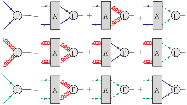
Figure 2: The coupled set of BSEs for two-body bound states of QCD. The blue, wiggly and dashed lines are the propagators for the quarks, gluons and ghots, respectively. The circles are the Bethe-Salpeter amplitudes $\Gamma$ and the boxes the scattering kernels $K$. Taken from Ref. [31].

A different approach consists in using the Bethe-Salpeter formalism. In principle, this allows to obtain information on bound states in a fully relativistic and non-perturbative manner. In practice, an infinite hierarchy of equations is involved, and approximations are needed to obtain results. In the Bethe-Salpeter equation (BSE), see Figure 2, one is interested in computing the amplitude $\Gamma$, given an ansatz for the the two-body irreducible scattering kernel $K$ and the form of quark, gluon and ghost propagators. In the absence of exact solutions for the latter, some kind of is needed, whose eventual effects are generally hard to control. Clearly, the choice of truncation and of the propagators becomes the crucial aspect in determining the solidity of this method.

The first attempt at the calculation of the $J=0$ glueball in the BSE framework can be found in Ref. [32]. Available lattice results on the behaviour of the gluon and ghost $2$-point function are used both to model vertices through their Schwinger-Dyson equations and to ensure the correctness of the resulting solution. These vertices are then used in truncated BSEs to predict the properties of glueballs. Assuming that the dressed version of the lowest order scattering kernel dominates the interaction and taking as input the mass of the scalar glueball computed in lattice simulations, the mass of the pseudoscalar glueball was obtained as $2.500(250)\leavevmode\nobreak\ GeV$. In Ref. [33, 34, 31], the BSEs were solved in in the Landau-gauge, in the pure Yang-Mills case. The truncation scheme at $3$-loops was consistent between the DSE for $2$-points functions and vertices, obtained from the $3$PI effective action. There is no external parameter dependency apart from an overall scale. The latter can be fixed by comparison with lattice results. The scalar and pseudoscalar glueball masses were estimated as $m(0^{++})=1.850(130)\,GeV$,$m(0^{-+})=2.580(180)\,GeV$ and $m(2^{++})=5.610(180)\,GeV$.

The large-$N_{c}$ approach plays an important role in that it allows to relate and combine results obtained at different values of $N_{c}$ with the phenomenologically relevant case $N_{c}=3$. It is based on the observation that the calculation of amplitudes in Yang-Mills theories drastically simplify when the number of colors $N_{c}$ is taken to infinity keeping $g^{2}N_{c}$ fixed. In particular, if the large-$N_{c}$ theory is a confining theory, then it describes stable and non-interacting mesons and glueballs, as can be easily understood from the scaling properties of Feynman diagrams with $N_{c}$. At $N_{c}$ large but finite, it is possible to show that,

$$\frac{m(J^{PC})}{\sqrt{\sigma}}=m(N_{c}=\infty)+\frac{c_{1}}{N_{c}^{2}}\leavevmode\nobreak\ ,$$ (8)

where the coefficient $c_{1}$ is independent of $N_{c}$. This approach rests on the possibility of computing the value of $m(N_{c}=\infty)$ and of $c_{1}$, which can be achieved in several different ways. For a lattice oriented review, see Ref. [35]. Related approaches have been adopted in the context of the Ads/CFT correspondence. They differ in the specific duality chosen, in the way the breaking of conformal symmetry is implemented, and in the identification of glueball operators. In the recent Ref. [36], the masses of the scalar and tensor glueballs are obtained in the context of the graviton soft wall model, in which the glueball is associated to a graviton propagating in $Ads_{5}$ space. The estimates of their masses are $m(0^{++})=1.920\,\mathrm{GeV}$ and $m(2^{++})=2.371\,\mathrm{GeV}$. For further results, see Section III.E of Ref. [37].

A summary of the above predictions for the spectrum of glueballs with quantum numbers $0^{++}$, $0^{-+}$ and $2^{++}$ channels is displayed in Figure 3.

Figure 3: The predictions on the spectrum of the $0^{++}$(scalar), $0^{-+}$(pseudo-scalar) and $2^{++}$(tensor) glueballs, from the phenomenological models reviewed in Section  2 (empty triangles) and from the analytical models reviewed in Section 3 (full triangles).

4 Lattice calculations

The numerical approach to lattice regularized quantum field theories is the only first principles approach to the exploration of the non-perturbative regime of QCD. As such, it is the instrument of choice for the study of glueballs, in particular their spectrum and the decay widths. In this section, estimates of the glueball spectral observables as theyr are usually obtained on the lattice are reviewed and the results present in the litterature are discussed.

The mass of a glueball state can be calculated from the large euclidean-time behaviour of correlators of operators with appropriate quantum numbers. For zero-momentum projected operators, under very broad assumptions,

$$C(t)=\langle\Omega|O(t)O^{\dagger}(0)|\Omega\rangle=\sum_{n}|c_{n}|^{2}e^{-m_{n}t}\leavevmode\nobreak\ ,$$ (9)

where $n$ labels the eigenstate of the Hamiltonian, the quantities $|c_{n}|^{2}=|\langle n|O_{i}(0)|\Omega\rangle|^{2}$ are known as overlaps, and $m_{n}$ are the masses in the channel with the same quantum numbers as the operator $O$. If there exists an isolated ground state of mass $m_{0}$ then, at sufficiently large $t$, the sum in Eq. 9 will be dominated by $|c_{0}|^{2}\exp{(-m_{0}t)}$. In principle, the mass can be obtained as,

$$m_{0}=-\lim_{t\to\infty}\frac{1}{t}\log{C(t)}\leavevmode\nobreak\ .$$ (10)

In practice, the computation of $m_{0}$ with the above form for $C(t)$ at finite values of $t$ will be affected by the contamination of higher energy states. The average value above can be computed on the lattice as an ensemble average and is defined schematically as,

$$C(t)=\frac{1}{Z}\int\mathcal{D}[U]\det M[U]\,O(t)O^{\dagger}(0)\,e^{-S_{\mathrm{YM}}[U]}\leavevmode\nobreak\ ,$$ (11)

where $M[U]$ is the fermion matrix, $S_{\mathrm{YM}}[U]$ is the action for the gluon field, and

$$Z=\int\mathcal{D}[U]\det M[U]e^{-S_{\mathrm{YM}}[U]}\leavevmode\nobreak\ .$$ (12)

Many different choices are possible for both $S_{\mathrm{YM}}[U]$ and $M[U]$. For example, both isotropic and anisotropic discretizations can be defined, and different actions characterized by different discretization errors.

At finite lattice spacing the states transform in irreducible representations of the symmetries of the system. These are known as channels. The channels are labelled by $R^{PC}$, where $R$ are irreducible representations of the octahedral group $O_{h}$, $P$ is spatial parity and $C$ is charge conjugation. There are $10$ possible channels, denoted by $A_{1}^{\pm},A_{2}^{\pm},E^{\pm},T_{1}^{\pm},T_{2}^{\pm}$. Their relationship with the continuum channels $J^{PC}$, which they become part of in the continuum limit, can be found in Table 1. States are generated from the (invariant) vacuum $|\Omega\rangle$ by gauge-invariant combinations of link variables and quark fields. Two families of such operators are known: traces of path-ordered products along closed lattice paths $U_{\mathcal{C}}={\mathrm{Tr}\leavevmode\nobreak\ }\leavevmode\nobreak\ \prod_{l\in\mathcal{C}}U_{l}$, and operators involving $q$ and $\bar{q}$ fields, $\bar{q}U_{\mathcal{L}}q$, where $\mathcal{L}$ is a path connecting $\bar{q}$ and $q$. The channel to which one operator belongs is dictated by the transformation properties of its support under elements of the octahedral group. As Charge conjugation simply amount to inverting the ordering of the link operators along a path, the representations with definite values of $C$ are simply obtained by considering the real and imaginary parts of ech $R^{P}$ representations.

$J$	$A_{1}$	$A_{2}$	$E$	$T_{1}$	$T_{2}$
$0$	$1$	$0$	$0$	$0$	$0$
$1$	$0$	$0$	$0$	$1$	$0$
$2$	$0$	$0$	$1$	$0$	$1$
$3$	$0$	$1$	$0$	$1$	$1$
$4$	$1$	$0$	$1$	$1$	$1$

Table 1: In the top row, the representations of the octahedral group. In the left column, the $J\leq 4$ representations of the Poincaré group. The elements $1$ of the matrix correspond to representations $R^{PC}$ that become part of representation $J$ in the continuum limit.

It was soon realized that glueball correlators are affected by a particularly severe signal-to-noise ratio problem. Two strategies have been proposed to overcome it. The first is based on the locality of both the Yang-Mills part of the action and the objective operator. It is known as multilevel, and allows to achieve an exponential reduction in the error of $C(t)$ at large $t$, see Refs. [38, 39]. Unfortunately, it rests on locality, and its use is limited to quenched theories. The second is known as variational method [40, 41]. A variational basis of operators $\left\{O_{i}\right\}$ is defined in a given channel, and their correlation matrix is obtained,

$$C_{ij}(t)=\langle\Omega|O_{i}(t)O_{j}(0)|\Omega\rangle=\sum_{n=1}^{\infty}c_{n,i}c_{n,j}e^{-m_{n}t}\leavevmode\nobreak\ ,$$ (13)

where $c_{n,i}=\langle n|O_{i}|\Omega\rangle$. By a diagonalization of $C_{ij}(t)$ at large $t$, the ground state $m_{0}$ can in principle be obtained. In practice, because of the presence of statistical fluctuations, one instead solves the GEVP, $C(t)v=\lambda(t,\,t_{0})C(t_{0})v$, at small $t$, where $v$ is a column vector, and $\lambda(t,\,t_{0})=e^{-m_{0}(t-t_{0})}$. This amounts to finding the linear combination $\Phi(t)=\sum_{i}v_{i}O_{i}(t)$ of the operators that maximize the overlap on the ground state in the channel. The mass can then be extracted from the large time behaviour of their correlator. The great majority of the estimates of the spectrum have been obtained using the variational method. The efficacy of the method depends crucially on the choice of the variational basis. An sample of the closed loop operators usually included is displayed in Figure 4. It has proved very effective to add to the variational basis operators calculated on blocked and smeared configurations [42, 43, 44]. This allows to better overlap with ground state configurations, especially in the vicinity of the continuum limit, where they are expected to be smooth on the $a$ scale. Moreover, as shown in Ref. [45], the construction of the variational basis can be automatized and the effect of scattering and di-torelon states that propagate in the correlator can be identified. Estimates of the glueball masses can thus be obtained at several values of the inverse coupling $\beta$, and on several lattice geometries $N_{s}^{2}\times N_{t}$ and provided other sources of systematicall error are addressed, an infinite volume continuum limit can then in principle be calculated.

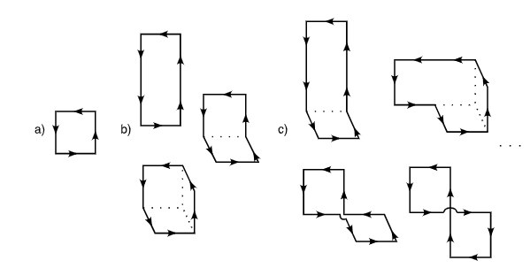
Figure 4: A sample of the lattice paths on which the glueball operators are defined. Taken from Ref. [45].

In quenched systems, where the fermionic degrees of freedom are infinitely massive and effectively static, the calculation of the glueball spectrum was one of the early successes of lattice QCD. It is nowadays one of the best known results obtained on the lattice, and a solid prediction from pure Yang-Mills theory. The spectrum can be calculated from the Wilson action on isotropic lattices, see Ref. [46], and from an improved action on anisotropic lattices, see Refs. [47, 48]. The high quality of these recent determinations of the spectrum rests on the careful identification of the target states and on the quality of the extrapolation to the continuum limit, and build upon decades of efforts.

The spectrum as obtained in Ref. [48] is displayed in Fig. 5. The picture confirms the results obtained in the majority of models: the lightest channels are the scalar, followed by the tensor and the pseudo-scalar channels. The scalar glueball in Ref. [48] has a mass of $1.710(80)\,GeV$, the pseudoscalar a mass of $2.560(120)\,GeV$ and the tensor $2.390(120)\,GeV$. In Ref. [46] the scalar glueball has mass $1.651(23)\,GeV$, the pseudoscalar $2.599(39)\,GeV$ and the tensor $2.378(31)\,GeV$. These predictions are compatible with each other within $1$-$\sigma$. Note that the choice of physical observables used to set the scale will have an effect on the final estimate in $GeV$ units. Estimates present in the litterature are often expressed in units of the Sommer’s scale $r_{0}$ or in units of $\sqrt{\sigma}$. In recent investigations, results in units of the Gradient Flow scale $t_{0}$ have started to appear.

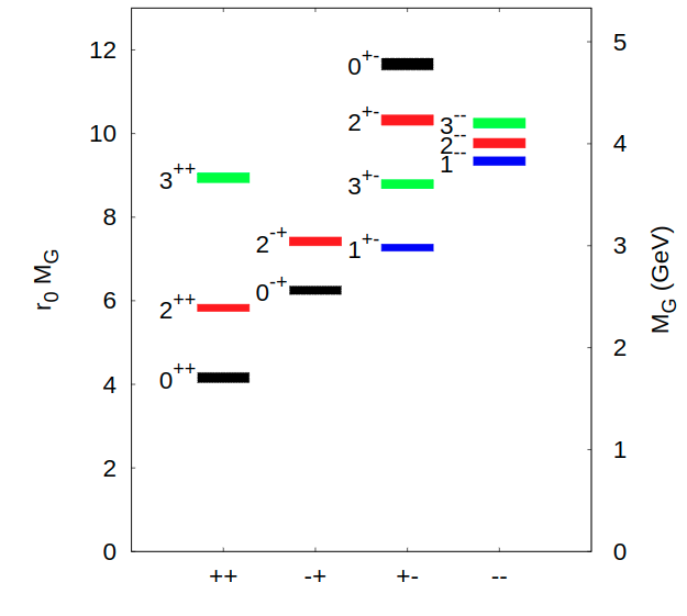
Figure 5: (left) The quenched spectrum, taken from Ref. [48]. (right) A summary of the results obtained in the scalar, pseudo-scalar and tensor channels in quenched systems. The numerical values are taken from Refs. [47, 48, 49, 50].

Quenched systems are also an ideal testbed to investigate both the quantitative effects of other sources of systematical error and to obtain the spectrum at larger values of $N_{c}$ or for different gauge groups. For example, topological freezing affects simulations performed with periodic boundary conditions at small values of $a$. The resulting loss of ergodicity might affect mass estimations, especially in the pseudoscalar channel. The problem has been analyzed at both $N_{c}=3$ and larger $N_{c}$, where the effect of topological freezing should be magnified, and found to be negligible, see Refs. [51, 52, 53, 54, 55]. Moreover, the spectrum was also evaluated at different values of the number of colors, see Ref. [56, 49, 45], and extrapolated to the limit $N_{c}\to\infty$. The lattice allows the exploration of the spectrum at large-$N_{c}$, see Ref. [45] Finally, the glueball spectrum was obtained for gauge theories based on other families of groups, see Ref. [57] for $Sp(N_{c})$ gauge theories. The comparison of spectral data for different families of gauge groups allows to analyze the degree of universality among Yang-Mills theories. In particular, the Casimir scaling and the universality of the ratio between the tensor and scalar glueball mass were analyzed in Refs. [58, 59].

A summary of the estimates of the spectrum in quenched lattice QCD is displayed in the right-hand panel of Figure 5.

The addition of dynamical fermions complicates the picture considerably. The vacuum is altered in way that is difficult to predict. Indeed, there is no reason to think that the unquenched and quenched spectra are similar: the presence of sea quarks of sufficiently low mass makes glueballs unstable, and the mixing with othere iso-singlet states makes it impossible to determine the very nature of the state under scrutiny. In other words, a glueball mixed with a $q\bar{q}$ component is indistinguishable from a meson with a glueball component. However, the possibility of varying the quark mass parameters smoothly in Lattice calculations affords us a crucial advantage, in that it allows us to tune the effects of the confounding phenomena above. In the regime of large quark masses, the system should be similar to its quenched limit, and the decays and mixing effects should be inhibited. Well defined glueballs and quarkonia states are expected, and their mass shouyld be calculable with the methods above. Reducing the sea quark mass smoothly reintroduces mixings and, for sufficiently small quark masses, decays.

Early studies on the unquenched glueball spectrum have been performed at $N_{f}=2$, with different fermion discretizations, in a regime of heavy quarks, see Refs. [60, 61, 62]. It is observed that, surprisingly, the statistical error in the determination of the correlators is smaller than expected. In Ref. [61], the masses of scalar and tensor glueballs at $N_{f}=2$ are obtained for Wilson fermions at $m_{\pi}\simeq 0.490\,\mathrm{GeV}$ and are compared with quenched results for similar values of the lattice spacing. They are found to be in agreement within errors. In Ref. [62], a similar calculation is carried out for non-perturbatively improved clover Wilson fermions at $m_{\pi}\simeq 0.3-0.6\,\mathrm{GeV}$. While the tensor glueball mass is found to be in agreement with the quenched predictions, while in the scalar channel it is found to be suppressed by $\sim 20\%$. As discussed by the authors, as this discrepancy seem to be independent of the value of the quark mass parameters, it might be explained as a lattice artifact introduced by the $O(a)$ improvement.

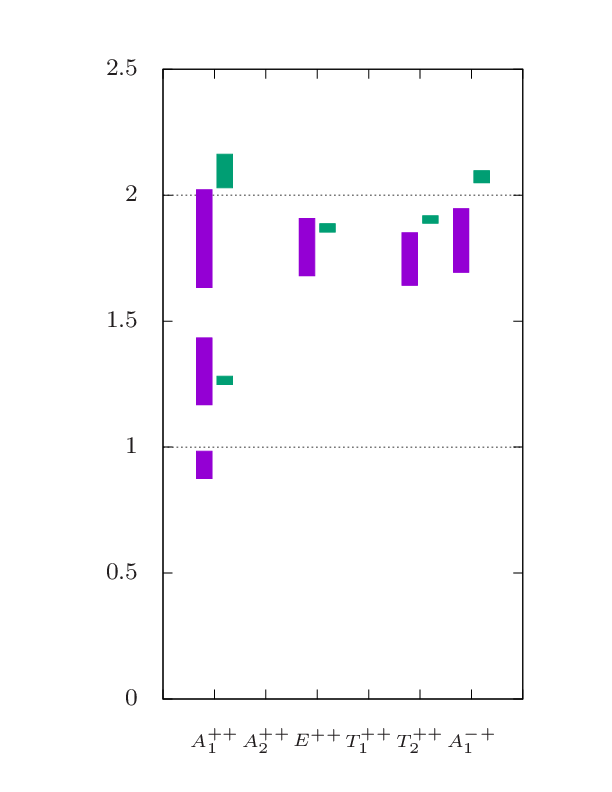
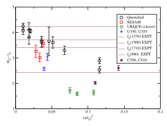
Figure 6: (left) In purple, the spectrum of glueballs for $N_{f}=4$ clover improved twisted mass fermions, in green, the quenched spectrum from Refs. [49, 46] $m_{\mathrm{PS}}\sim 250\leavevmode\nobreak\ \mathrm{MeV}$. Taken from Ref. [63]. (right) Quenched and Unquenched spectrum of the scalar glueball at finite $a$ and various values of $m_{\pi}$. The green diamonds are from Ref. [62], the blue and purple crosses from Ref. [64], the red squares from Ref. [61]. The quenched results from Ref. [47] are represnted as black circles. Taken from Ref. [64].

The above results were obtained with only pure-glue operators in the variational basis. In Ref. [65], $q\bar{q}$ operators were included in the variational basis and the mass of the flavor-singlet state was measured in a system with $N_{f}=2$ flavors of clover improved Wilson fermions. A suppression was observed in the mass of the flavor-singlet scalar state with respect to the results of Refs. [61, 62]. Note that no difference was found between the mass obtained from a purely gluonic variational basis and from a mixed one. In order to interpret this suppression, the same calculation was performed in Ref. [64] in two different ways. First, using the same action but at a finer lattice, and also using interpolating operators at non-zero momentum. Second, on ensembles generated by a gauge improved Iwasaki action. In both cases, the suppression was still observed, see Figure 6. Two different interpretations thereof are put forward in Ref. [64]. The suppression could be an artifact of the lattice discretization, caused by the so-called "scalar dip", or it could be a genuine effect of mixing. The masses of glueballs in the scalar, pseudo-scalar and tensor channels were later obtained for $2+1$ flavors of improved staggered fermions in Ref. [66] and with a purely gluonic variational basis. Only a weak dependence on the lattice spacing was found and the values of the masses were found to be compatible with their value in the quenched continuum limit. The addition of scattering states to the variational basis did not alter this conclusion, see Ref. [67].

More recently, these masses were computed using a purely gluonic variational basis for an anisotropic lattice with $N_{f}=2$ clover-improved Wilson fermions in Ref. [68]. No unquenching effects were detected on the masses of the pseudo-scalar and tensor channels. The scalar channel appears to have a slightly suppressed mass with respect to its quenched counterpart. However, no continuum limit is considered and more investigations are needed before relating this effect to mixing. The scalar glueball was the focus of Ref. [69], where for the first time, two-hadrons ($\pi\pi$, $K\bar{K}$ and $\eta\eta$), $q\bar{q}$ and purely-gluonic operators were included in the variational basis. A single ensemble of $N_{f}=2+1$ clover improved Wilson fermions was analyzed at $m_{\pi}\sim 390\,MeV$, using the stochastic LapH method to evaluate all-to-all quark propagation. The aim of the authors was to understand whether, starting from the light hadron spectrum obtained from only linear combinations of fermionic operators, additional states were observed to appear upon inclusion of glueball operators in the variational basis. Curiously, no new state appears within the energy range considered. This is an indication that further study is needed on the effects systematics introduced by the choice of the variational basis.

Figure 7: A summary of estimates of the unquenched glueball spectrum. In light blue, the results from Ref. [61], in light orange and green, the results from Ref. [68], in red, the results in Ref. [70], in purple the results from Ref. [67], in brown, the results from Ref. [63], in cyan the quenched results from Ref. [48].

At this conference, a calculation of the scalar glueball mass with $N_{f}=4$ clover improved twisted mass fermions was presented, see Ref. [63]. The low-quark mass regime was explored, with $m_{\pi}\sim 250\,MeV$ and while in the pseudo-scalar and tensor channel the masses were roughly found to agree with the corresponding quenched values, a new light state was observed in the scalar channel. Notably, the mass of the first and second excited states was found to be similar to that the ground state and first excited quenched glueballs, respectively. The spectrum is displayed in in the left-hand panel of Figure 6. It is suggested that the new low-lying state is $\pi\pi$ or a $q\bar{q}$ state. A similar calculation was performed for $N_{f}=2+1+1$. The fact that the mass of the additional low-lying state was shown to depend strongly on $m_{\pi}$ suggests that it might contain a large quark content. The above results illustrate the need to improve our understanding of the unquenched glueball spectrum, especially in the continuum limit. However, the most pressing questions are on the effects of mixing.

A summary of the estimates of the spectrum in unquenched lattice QCD at finite lattice spacing is displayed in Figure 7.

The formalism to study the effects of mixing on the spectrum was described in detail in Ref. [65] where the mixing is found to be substantial. The same analysis was improved and obtained at smaller lattice spacing in Ref. [64], with non-perturbatively improved clover fermions at $a\sim 0.1\,fm$. In Ref. [66], an approximated value of the non-diagonal element of the mixing matrix was obtained in a system of $N_{f}=2+1$ improved staggered fermions, with $m_{\pi}\sim 280\,MeV$ and $m_{\pi}\sim 360\,MeV$. While the behaviour of the mixed correlation function was in agreement with expectations, the data was still too noisy to draw any quantitative conclusion. Recently, the problem of computing the disconnected contribution to the mixed correlators has received some attention. In Ref. [71, 72], the distillation method was used in a system with $N_{f}=2$ heavy quarks. In Ref. [73], $N_{f}=2$ flavors of heavy quarks are considered on an anisotropic lattice. The mixing energy is computed from the explicit calculation of mixed glueball-quarkonia correlators. A mixing energy of $49(6)\,MeV$ and a mixing angle of $|\theta|=4.3(4)^{\circ}$ are obtained. A similar study was performed in Ref. [74] using distillation to compute the values of the disconnected diagrams involved in the mixing dynamics. A system of $N_{f}=2$ flavors of clover improved fermions on an anisotropic lattice at $m_{\pi}\sim 350\,MeV$ was considered. The mixing energy was found to be $107(14)\,MeV$ and the mixing angle was estimated to be $|\theta|=2.47(46)^{\circ}$; this is small enough to argue that the mixing effects can be largely ignored in the pseudo-scalar channel at $N_{f}=2$.

A summary of the estimates of the spectrum in unquenched lattice QCD at finite lattice spacing is displayed in Figure 7.

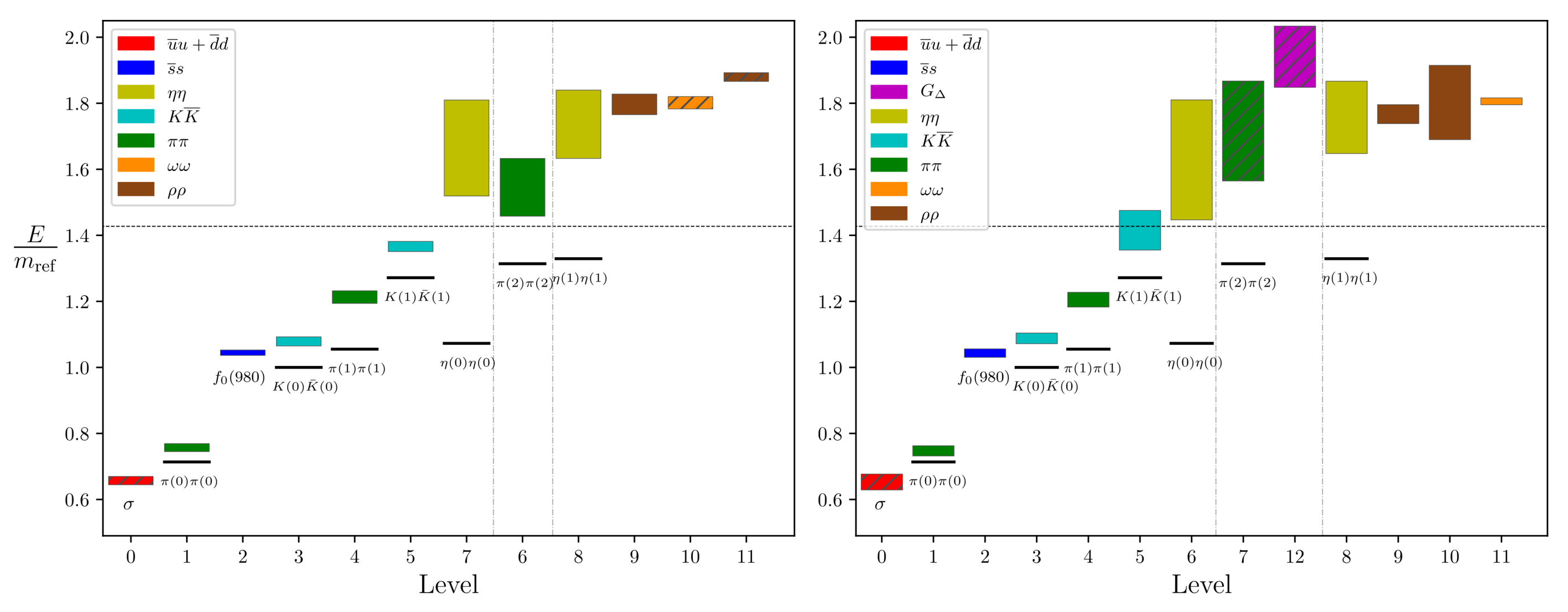
Figure 8: The spectrum of light hadrons without (left) and with (right) glueball operators in the variational basis, with $m_{\mathrm{ref}}=2m_{\mathrm{K}}$. Taken from Ref. [69].

The prediction of the decay width of glueballs from QCD is crucial to the comparison with experiments and is tightly related to the problem of determining the mixing between glueballs and other iso-singlet states. A glueball with a very small decay width would already have been identified, while a very large resonance could remain out of reach forever.

The calculation of decay widths from lattice QCD is notoriously difficult and numerically very expensive. Despite the recent progresses in computing decay widths for mesons using the Lüscher-Lellouch method, see Ref. [75], much remains to be done before this method can be fruitfully used for glueballs. The main difficulty in the case of glueballs lies in the fact that, since glueballs are iso-singlet states, studying their mixing with $q\bar{q}$ state will necessarily involve the computation of correlators corresponding to disconnected diagrams. Decays glueballs to a pair of pseudo-scalar mesons were first studied in Refs. [76, 77]. The $2$-point functions of purely gluonic states with two-body meson operators at zero and non-zero value of the back-to-back momentum were studied in the quenched approximation. The width of the decay to two pseudo-scalars was obtained as $108(29)\,MeV$ and the total decay width was estimate to be smaller than $200\,MeV$, which would make the glueball well identifiable in experiments. Related to the decay of glueballs to other states is the decay of the $J/\psi$ to glueballs. In Ref. [78, 79, 80], the estimates of the decay widths to a photon plus a glueball are given for the scalar, pseudo-scalar and tensor channel in the quenched approximation and on anisotropic lattices, using the formalism described in Ref. [81]. A width of $0.35(8),\,keV$ is found, corresponding to a branching ratio of $3.8(9)\times 10^{-3}$ for the scalar glueball. A width of $1.01(22)(10),keV$, corresponding to a branching ratio of $1.1(2)\times 10^{-2}$ for the tensor glueball. A width of $0.0215(74),\,keV$, corresponding to a branching ratio of $2.31(80)\times 10^{-4}$ for the pseudo-scalar glueball. The study of the potential between glueballs and their scattering is a related and relevant problem, i.e. for models of glueball dark matter. In this respect, see Refs. [82, 83].

5 Experimental results

The detection of glueball states is one of the long standing unsolved problems in hadron spectroscopy. Several strategies have been developed in order to identify a signal that could confirm their existence and a large number of studies have been conducted with that aim. For recent review, see Ref. [84, 85, 86].

The typical experimental signature expected from a glueball is the appearance of supernumerary states, that do not fit into the $q\bar{q}$ nonets of the minimal quark model. Their decay should exhibit branching fractions that are incompatible with those expected from $SU(3)$,

$$\pi\pi:K\bar{K}:\eta\eta:\eta\eta^{\prime}=3:4:1:0\leavevmode\nobreak\ ,$$ (14)

and their detection should be best visible in Gluon-rich channels. The latter are processes in which the not involving a glueball are suppressed, for example by the OZI-rule. The two confounding effects that have prevented the identification of a glueball signal so far are the mixing mentioned above on which, unfortunately, little is known, and the possible presence of decay form factors.

Three examples of gluon-rich channels that are currently under scrutiny in search of a glueball are displayed in Figure 9. The $\bar{p}p$ annihilation is represented on the right-hand panel, a $q\bar{q}$ pair can annihilate and a glueball may be formed. This reaction was studied at the Crystal Barrel experiment, see Ref. [87], and will be the focus of the future PANDA experiment at FAIR, see Refs. [88] for a discussion involving the scalar glueball. The diffractive scattering of hadrons is represented in the centre panel, and also known as double pomeron exchange. Since no valence quarks are exchanged, a glueball may form. This reaction was studied at the WA102 experiment. The radiative decay of the $J/\psi$ resonance is represented on the left-hand panel. In this case, the OZI rule suppresses decay into light quarks, and the interesting process if the decay to a (detectable) photon and a pair of gluons. The pair of gluons might form a glueball, and its decay to a pair of mesons might be identified. The BESIII experiment is currently collecting data on this process.

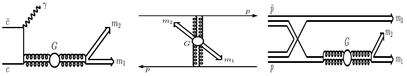
Figure 9: A sketch of three examples of Gluon rich processes. In the left hand panel, the radiative decay $J/\psi\to\gamma mm$, where $m$ is a meson. In the centre panel, pomeron-pomeron collision, and in the right hand panel, hadron central production. Taken from Ref. [84]

Below, the focus is on the scalar sector, which is the most controversial. The number of states observed under $\sim 2.5\,GeV$ is still debated and so is their identification. The states in this channel are listed in Table 3. Among those, $9$ are listed in the 2020 issue of the PDG. The $f_{0}(500)$ and $f_{0}(980)$ have been mainly interpreted as molecular states. The states $f_{0}(1370)$, $f_{0}(1500)$ where established by the Cristal Barrel experiment through their decays to $\eta\eta$ and $\pi^{0}\pi^{0}$. Neither have large coupling to $K\bar{K}$, and this would indicate that they cannot have a large $s\bar{s}$ component. The results from the WA102 experiment are in agreement with this view. The state $f_{0}(1710)$ was reported to decay predominantly to $K\bar{K}$, indicating that it is predominantly $s\bar{s}$. Clearly, not all of these states can be scalar iso-scalars, and one of them must be supernumerary. The fact that experiments at LEP have indicated that the $f_{0}(1500)$ is practically absent from $\gamma\gamma\to K\bar{K}$ and $\gamma\gamma\to\pi^{+}\pi^{-}$ decays would suggest that it is predominantly $s\bar{s}$, in contradiction with the above picture. The $f_{0}(1500)$ is thus thought to be supernumerary. Yet the pattern of its decays to $\pi\pi$, $\eta\eta$, $\eta^{\prime}\eta^{\prime}$ and $K\bar{K}$ indicate that it cannot be a pure glueball either. This points to the idea that the $f_{0}(1500)$ is a mixed state, partly glueball partly $q\bar{q}$.

Many studies revolve around the idea of mixing first explored in Ref. [89] for the scalar sector. Let $|G\rangle$, $|n\bar{n}\rangle$ and $|s\bar{s}\rangle$, be the bare states, where $|n\bar{n}\rangle=(|u\bar{u}\rangle+|d\bar{d}\rangle)/\sqrt{2}$ and let $M$ be the mass matrix,

$$M=\begin{bmatrix}M_{G}&f&\sqrt{2}f\\ f&M_{S}&0\\ \sqrt{2}f&0&M_{N}\end{bmatrix},\quad f=\langle s\bar{s}|V|G\rangle=\langle n\bar{n}|V|G\rangle/\sqrt{2}\leavevmode\nobreak\ ,$$ (15)

and $V$ is the potential generating the mixing. Then, the observed states, i.e. the $f_{0}(1370)$, $f_{0}(1500$ and $f_{0}(1710)$ are the eigenvalues of $M$.

Mixing also underlies the idea of a distributed glueball, put forward in Refs. [90, 91]. In this case, the various resonances in Table 3 are ascribed either to a singlet or to a octet of $SU(3)$. Their assignement can for example be decided from their Regge trajectories. While octet mesons should not appear in radiative decays of the $J/\psi$, they are abundantly produced. Moreover, singlets should be produced, but their yield shows a peak at $\sim 1.865\,GeV$. This enhancement is interpreted as a scalar glueball mixed into the wave-function of mainly-octet and mainly-singlet mesons.

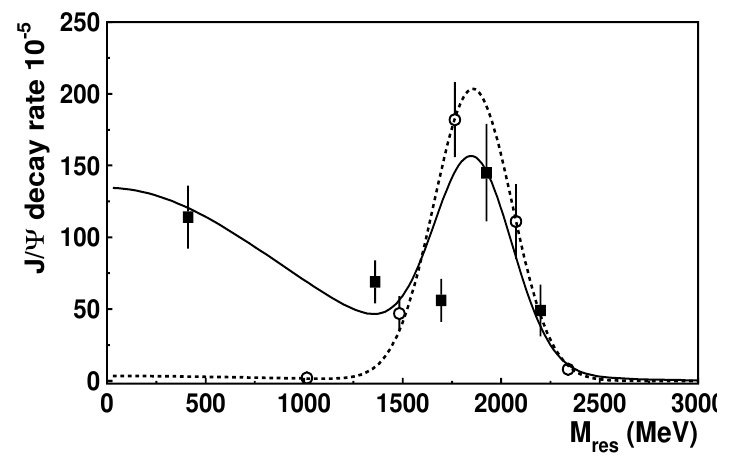
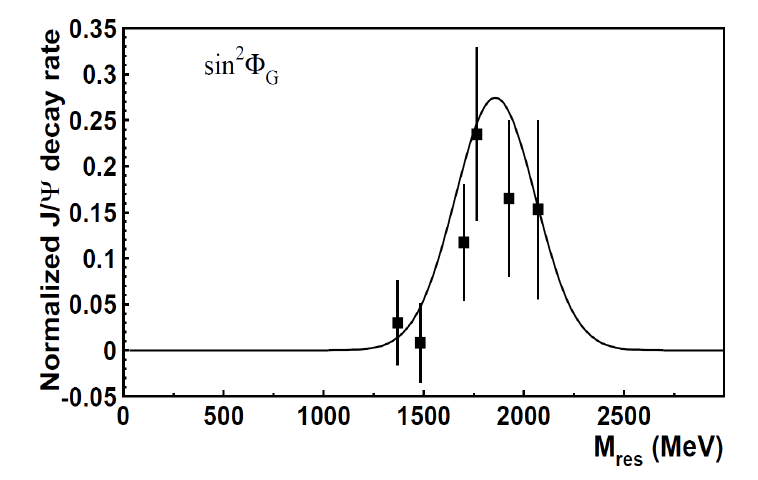
Figure 10: In the left-hand panel, the yield of mainly octet(circle) and mainly-singlet(squares) mesons in the radiative $J/\psi$ decays, plotted as a function of the mass $M_{\mathrm{res}}$ of the resonance. In the right-hand panel, the glueball content of the resonances as a function of $M_{\mathrm{res}}$. The solid line is a Breit-Wigner distribution normalized to unit area, while the black squares are the values of $\sin^{2}\phi_{n}^{s}$, where $\phi_{n}^{s}$ is the mixing angle between non-glue states. Note that the distribution of yields and the distribution of the glueball across the resonances is the same. Taken from Refs. [90].

res.	$f_{0}(1370)$	$f_{0}(1500)$	$f_{0}(1710)$	$f_{0}(1770)$	$f_{0}(2020)$	$f_{0}(2100)$
G fraction	$5(4)\%$	$<5\%$	$12(6)\%$	$25(10)\%$	$16(9)\%$	$17(8)\%$

Table 2: The glueball fraction found from a coupled-channel analysis of the decays of the $J/\psi$ into $\gamma\pi^{0}\pi^{0}$, $\gamma K_{S}K_{S}$, $\gamma\eta\eta$ and $\gamma\phi\omega$. Taken from Ref. [90].

In particular, a coupled channel analysis of the decays of $J/\psi$ into $\gamma\pi^{0}\pi^{0}$, $\gamma K_{S}K_{S}$, $\gamma\eta\eta$ and $\gamma\phi\omega$ indicates that a tenth state, the $f_{0}(1770)$ is required to fit the invariant mass distributions of these decay products. The pole masses and width were obtained with the K-matrix approach, and the glueball contents of the resonances could be determined. They are reported in Table 2. Note that the fractions only amount to $\sim 78\%$ with a small fraction expected from $f_{0}(2020)$ and $f_{0}(2100)$. This indicates the presence of a “fractional glueball” and to argue for a distributed scalar glueball with $m(0^{++})=1.865(50),\mathrm{GeV}$ and decay rate $\Gamma\sim 0.370(50)\,\mathrm{GeV}$.

name	$m(\mathrm{MeV})$	$\Gamma(\mathrm{MeV})$
$f_{0}(500)\bullet$	$400\to 500$	$480(30)$
$f_{0}(980)\bullet$	$990(1)20$	$71(10)$
$f_{0}(1370)\bullet$	$1200\to 1500$	$200\to 500$
$f_{0}(1500)\bullet$	$1506(6)$	$112(9)$
$f_{0}(1710)\bullet$	$1704(12)$	$123(18)$
$f_{0}(1770)$	$1765(15)$	$180(20)$
$f_{0}(2020)\bullet$	$1992(16)$	$442(60)$
$f_{0}(2100)\bullet$	$2086^{20}_{-24}$	$284^{60}_{32}$
$f_{0}(2200)\bullet$	$2187(14)$	$\sim 200$
$f_{0}(2330)\bullet$	$\sim 2330$	$250(20)$

Table 3: The masses and decay widths of the ten scalar iso-scalar resonances considered in the text. The bullets indicate those that are confirmed in Ref. [92]. The additional resonance $f_{0}(1770)$ was first proposed in Ref. [93] and is argued in Ref. [90] to be the tenth isoscalar resonance.

6 Conclusion

Glueballs are among the predictions of QCD that still await undisputed confirmations. Many different phenomenological models, more or less QCD inspired predict masses that are similar, and in agreement with Lattice QCD results, obtained in the quenched approximation

$$m(0^{++})=1.6(1)\,GeV,\quad m(2^{++})=2.4(1)\,GeV,\quad m(2^{++})=2.5(1)\,GeV,\quad$$ (16)

and $\Gamma\simeq 0.1\,GeV$ for the decay width.

Unquenched results, that are numerically more expensive, are also affected by obscuring effects, mixing and decays, and a first principles study that includes a continuum extrapolation at the physical pion mass is still lacking. Decay widths have been calculated but are affected by large systematical errors.

The experimental situation is debated. There is agreement on the present of a supernumerary state in the scalar iso-scalar channel, but several scenarios, based on the idea of mixing, are equally plausible for the identification of the scalar glueball. Further information, coming from the currently running BESIII experiment might prove useful.

References

- [1] Harald Fritzsch and Murray Gell-Mann. Current algebra: Quarks and what else? eConf, C720906V2:135–165, 1972.
- [2] R. L. Jaffe, K. Johnson, and Z. Ryzak. Qualitative Features of the Glueball Spectrum. Annals Phys., 168:344, 1986.
- [3] L. D. Landau. On the angular momentum of a system of two photons. Dokl. Akad. Nauk SSSR, 60(2):207–209, 1948.
- [4] Chen-Ning Yang. Selection Rules for the Dematerialization of a Particle Into Two Photons. Phys. Rev., 77:242–245, 1950.
- [5] Ted Barnes. A Transverse Gluonium Potential Model With Breit-fermi Hyperfine Effects. Z. Phys. C, 10:275, 1981.
- [6] John M. Cornwall. Dynamical Mass Generation in Continuum QCD. Phys. Rev. D, 26:1453, 1982.
- [7] Arlene C. Aguilar and Joannis Papavassiliou. Gluon mass generation in the PT-BFM scheme. JHEP, 12:012, 2006.
- [8] J. M. Cornwall and A. Soni. Glueballs as Bound States of Massive Gluons. Phys. Lett. B, 120:431, 1983.
- [9] Claude W. Bernard. Monte Carlo Evaluation of the Effective Gluon Mass. Phys. Lett. B, 108:431–434, 1982.
- [10] Vincent Mathieu, Fabien Buisseret, and Claude Semay. Gluons in glueballs: Spin or helicity? Phys. Rev. D, 77:114022, 2008.
- [11] A. Chodos, R. L. Jaffe, K. Johnson, Charles B. Thorn, and V. F. Weisskopf. A New Extended Model of Hadrons. Phys. Rev. D, 9:3471–3495, 1974.
- [12] R. L. Jaffe and K. Johnson. Unconventional States of Confined Quarks and Gluons. Phys. Lett. B, 60:201–204, 1976.
- [13] K. Johnson. The M.I.T. Bag Model. Acta Phys. Polon. B, 6:865, 1975.
- [14] C. Rebbi. Nonspherical Deformations of Hadronic Bags. Phys. Rev. D, 12:2407, 1975.
- [15] Michael S. Chanowitz and Stephen R. Sharpe. Hybrids: Mixed States of Quarks and Gluons. Nucl. Phys. B, 222:211–244, 1983. [Erratum: Nucl.Phys.B 228, 588–588 (1983)].
- [16] C. E. Carlson, T. H. Hansson, and C. Peterson. Meson, Baryon and Glueball Masses in the MIT Bag Model. Phys. Rev. D, 27:1556–1564, 1983.
- [17] Nathan Isgur and Jack E. Paton. A Flux Tube Model for Hadrons. Phys. Lett. B, 124:247–251, 1983.
- [18] Nathan Isgur and Jack E. Paton. A Flux Tube Model for Hadrons in QCD. Phys. Rev. D, 31:2910, 1985.
- [19] Mikhail A. Shifman, A. I. Vainshtein, and Valentin I. Zakharov. QCD and Resonance Physics. Theoretical Foundations. Nucl. Phys. B, 147:385–447, 1979.
- [20] Mikhail A. Shifman, A. I. Vainshtein, and Valentin I. Zakharov. QCD and Resonance Physics: Applications. Nucl. Phys. B, 147:448–518, 1979.
- [21] Mikhail A. Shifman. Snapshots of hadrons or the story of how the vacuum medium determines the properties of the classical mesons which are produced, live and die in the QCD vacuum. Prog. Theor. Phys. Suppl., 131:1–71, 1998.
- [22] V. A. Novikov, Mikhail A. Shifman, A. I. Vainshtein, and Valentin I. Zakharov. eta-prime Meson as Pseudoscalar Gluonium. Phys. Lett. B, 86:347, 1979.
- [23] V. A. Novikov, Mikhail A. Shifman, A. I. Vainshtein, and Valentin I. Zakharov. In a Search for Scalar Gluonium. Nucl. Phys. B, 165:67–79, 1980.
- [24] Stephan Narison. Spectral Function Sum Rules for Gluonic Currents. Z. Phys. C, 26:209, 1984.
- [25] Stephan Narison. Masses, decays and mixings of gluonia in QCD. Nucl. Phys. B, 509:312–356, 1998.
- [26] Thomas Schäfer and Edward V. Shuryak. Glueballs and instantons. Phys. Rev. Lett., 75:1707–1710, 1995.
- [27] Hilmar Forkel. Scalar gluonium and instantons. Phys. Rev. D, 64:034015, 2001.
- [28] Hilmar Forkel. Direct instantons, topological charge screening and QCD glueball sum rules. Phys. Rev. D, 71:054008, 2005.
- [29] Hua-Xing Chen, Wei Chen, and Shi-Lin Zhu. Two- and three-gluon glueballs of C=+. Phys. Rev. D, 104(9):094050, 2021.
- [30] Hua-Xing Chen, Wei Chen, and Shi-Lin Zhu. Two- and three-gluon glueballs within QCD sum rules. Nucl. Part. Phys. Proc., 318-323:122–126, 2022.
- [31] Markus Q. Huber, Christian S. Fischer, and Helios Sanchis-Alepuz. Glueballs from bound state equations. EPJ Web Conf., 274:03016, 2022.
- [32] Joseph Meyers and Eric S. Swanson. Spin Zero Glueballs in the Bethe-Salpeter Formalism. Phys. Rev. D, 87(3):036009, 2013.
- [33] Markus Q. Huber, Christian S. Fischer, and Hèlios Sanchis-Alepuz. Spectrum of scalar and pseudoscalar glueballs from functional methods. Eur. Phys. J. C, 80(11):1077, 2020.
- [34] Markus Q. Huber, Christian S. Fischer, and Helios Sanchis-Alepuz. Higher spin glueballs from functional methods. Eur. Phys. J. C, 81(12):1083, 2021. [Erratum: Eur.Phys.J.C 82, 38 (2022)].
- [35] Biagio Lucini and Marco Panero. SU(N) gauge theories at large N. Phys. Rept., 526:93–163, 2013.
- [36] Matteo Rinaldi and Vicente Vento. Meson and glueball spectroscopy within the graviton soft wall model. Phys. Rev. D, 104(3):034016, 2021.
- [37] Vincent Mathieu, Nikolai Kochelev, and Vicente Vento. The Physics of Glueballs. Int. J. Mod. Phys. E, 18:1–49, 2009.
- [38] Harvey B. Meyer. Locality and statistical error reduction on correlation functions. JHEP, 01:048, 2003.
- [39] Michele Della Morte and Leonardo Giusti. A novel approach for computing glueball masses and matrix elements in Yang-Mills theories on the lattice. JHEP, 05:056, 2011.
- [40] Kenneth G. Wilson. Confinement of Quarks. Phys. Rev. D, 10:2445–2459, 1974.
- [41] K. Ishikawa, M. Teper, and G. Schierholz. The Glueball Mass Spectrum in QCD: First Results of a Lattice Monte Carlo Calculation. Phys. Lett. B, 110:399–405, 1982.
- [42] M. Albanese et al. Glueball Masses and String Tension in Lattice QCD. Phys. Lett. B, 192:163–169, 1987.
- [43] M. Teper. An Improved Method for Lattice Glueball Calculations. Phys. Lett. B, 183:345, 1987.
- [44] Biagio Lucini, Michael Teper, and Urs Wenger. Glueballs and k-strings in SU(N) gauge theories: Calculations with improved operators. JHEP, 06:012, 2004.
- [45] Biagio Lucini, Antonio Rago, and Enrico Rinaldi. Glueball masses in the large N limit. JHEP, 08:119, 2010.
- [46] Andreas Athenodorou and Michael Teper. The glueball spectrum of SU(3) gauge theory in 3 + 1 dimensions. JHEP, 11:172, 2020.
- [47] Colin J. Morningstar and Mike J. Peardon. The Glueball spectrum from an anisotropic lattice study. Phys. Rev. D, 60:034509, 1999.
- [48] Y. Chen et al. Glueball spectrum and matrix elements on anisotropic lattices. Phys. Rev. D, 73:014516, 2006.
- [49] Andreas Athenodorou and Michael Teper. SU(N) gauge theories in 3+1 dimensions: glueball spectrum, string tensions and topology. JHEP, 12:082, 2021.
- [50] Harvey B. Meyer and Michael J. Teper. Glueball Regge trajectories and the pomeron: A Lattice study. Phys. Lett. B, 605:344–354, 2005.
- [51] Abhishek Chowdhury, A. Harindranath, and Jyotirmoy Maiti. Open Boundary Condition, Wilson Flow and the Scalar Glueball Mass. JHEP, 06:067, 2014.
- [52] Abhishek Chowdhury, A. Harindranath, and Jyotirmoy Maiti. Correlation and localization properties of topological charge density and the pseudoscalar glueball mass in SU(3) lattice Yang-Mills theory. Phys. Rev. D, 91(7):074507, 2015.
- [53] Alessandro Amato, Gunnar Bali, and Biagio Lucini. Topology and glueballs in Yang-Mills with open boundary conditions. PoS, LATTICE2015:292, 2016.
- [54] Claudio Bonanno, Massimo D’Elia, Biagio Lucini, and Davide Vadacchino. Towards glueball masses of large- Yang-Mills theories without topological freezing via parallel tempering on boundary conditions. PoS, LATTICE2022:392, 2023.
- [55] Claudio Bonanno, Massimo D’Elia, Biagio Lucini, and Davide Vadacchino. Towards glueball masses of large- pure-gauge theories without topological freezing. Phys. Lett. B, 833:137281, 2022.
- [56] B. Lucini and M. Teper. SU(N) gauge theories in four-dimensions: Exploring the approach to N = infinity. JHEP, 06:050, 2001.
- [57] Ed Bennett, Jack Holligan, Deog Ki Hong, Jong-Wan Lee, C. J. David Lin, Biagio Lucini, Maurizio Piai, and Davide Vadacchino. Glueballs and strings in Yang-Mills theories. Phys. Rev. D, 103(5):054509, 2021.
- [58] Ed Bennett, Jack Holligan, Deog Ki Hong, Jong-Wan Lee, C. J. David Lin, Biagio Lucini, Maurizio Piai, and Davide Vadacchino. Color dependence of tensor and scalar glueball masses in Yang-Mills theories. Phys. Rev. D, 102(1):011501, 2020.
- [59] Deog Ki Hong, Jong-Wan Lee, Biagio Lucini, Maurizio Piai, and Davide Vadacchino. Casimir scaling and Yang–Mills glueballs. Phys. Lett. B, 775:89–93, 2017.
- [60] Khalil M. Bitar et al. On glueballs and topology in lattice QCD with two light flavors. Phys. Rev. D, 44:2090–2109, 1991.
- [61] Gunnar S. Bali, Bram Bolder, Norbert Eicker, Thomas Lippert, Boris Orth, Peer Ueberholz, Klaus Schilling, and Thorsten Struckmann. Static potentials and glueball masses from QCD simulations with Wilson sea quarks. Phys. Rev. D, 62:054503, 2000.
- [62] A. Hart and M. Teper. On the glueball spectrum in O(a) improved lattice QCD. Phys. Rev. D, 65:034502, 2002.
- [63] Andreas Athenodorou, Jacob Finkenrath, Adam Lantos, and Michael Teper. The glueball spectrum with light fermions. PoS, LATTICE2022:057, 2023.
- [64] A. Hart, C. McNeile, Christopher Michael, and J. Pickavance. A Lattice study of the masses of singlet 0++ mesons. Phys. Rev. D, 74:114504, 2006.
- [65] Craig McNeile and Christopher Michael. Mixing of scalar glueballs and flavor singlet scalar mesons. Phys. Rev. D, 63:114503, 2001.
- [66] Christopher M. Richards, Alan C. Irving, Eric B. Gregory, and Craig McNeile. Glueball mass measurements from improved staggered fermion simulations. Phys. Rev. D, 82:034501, 2010.
- [67] E. Gregory, A. Irving, B. Lucini, C. McNeile, A. Rago, C. Richards, and E. Rinaldi. Towards the glueball spectrum from unquenched lattice QCD. JHEP, 10:170, 2012.
- [68] Wei Sun, Long-Cheng Gui, Ying Chen, Ming Gong, Chuan Liu, Yu-Bin Liu, Zhaofeng Liu, Jian-Ping Ma, and Jian-Bo Zhang. Glueball spectrum from lattice QCD study on anisotropic lattices. Chin. Phys. C, 42(9):093103, 2018.
- [69] Ruairí Brett, John Bulava, Daniel Darvish, Jacob Fallica, Andrew Hanlon, Ben Hörz, and Colin Morningstar. Spectroscopy From The Lattice: The Scalar Glueball. AIP Conf. Proc., 2249(1):030032, 2020.
- [70] Feiyu Chen, Xiangyu Jiang, Ying Chen, Keh-Fei Liu, Wei Sun, and Yi-Bo Yang. Glueballs at Physical Pion Mass. 11 2021.
- [71] Juan Andrés Urrea Niño, Francesco Knechtli, Tomasz Korzec, and Mike Peardon. Optimizing distillation for charmonium and glueballs. PoS, LATTICE2021:314, 2022.
- [72] Francesco Knechtli, Tomasz Korzec, Michael Peardon, and Juan Andrés Urrea-Niño. Optimizing creation operators for charmonium spectroscopy on the lattice. Phys. Rev. D, 106(3):034501, 2022.
- [73] Renqiang Zhang, Wei Sun, Ying Chen, Ming Gong, Long-Cheng Gui, and Zhaofeng Liu. The glueball content of c. Phys. Lett. B, 827:136960, 2022.
- [74] Xiangyu Jiang, Wei Sun, Feiyu Chen, Ying Chen, Ming Gong, Zhaofeng Liu, and Renqiang Zhang. -glueball mixing from lattice QCD. 5 2022.
- [75] Laurent Lellouch and Martin Luscher. Weak transition matrix elements from finite volume correlation functions. Commun. Math. Phys., 219:31–44, 2001.
- [76] J. Sexton, A. Vaccarino, and D. Weingarten. Scalar glueball decay. Nucl. Phys. B Proc. Suppl., 42:279–281, 1995.
- [77] J. Sexton, A. Vaccarino, and D. Weingarten. Numerical evidence for the observation of a scalar glueball. Phys. Rev. Lett., 75:4563–4566, 1995.
- [78] Long-Cheng Gui, Ying Chen, Gang Li, Chuan Liu, Yu-Bin Liu, Jian-Ping Ma, Yi-Bo Yang, and Jian-Bo Zhang. Scalar Glueball in Radiative Decay on the Lattice. Phys. Rev. Lett., 110(2):021601, 2013.
- [79] Yi-Bo Yang, Long-Cheng Gui, Ying Chen, Chuan Liu, Yu-Bin Liu, Jian-Ping Ma, and Jian-Bo Zhang. Lattice Study of Radiative J/ Decay to a Tensor Glueball. Phys. Rev. Lett., 111(9):091601, 2013.
- [80] Long-Cheng Gui, Jia-Mei Dong, Ying Chen, and Yi-Bo Yang. Study of the pseudoscalar glueball in radiative decays. Phys. Rev. D, 100(5):054511, 2019.
- [81] Jozef J. Dudek, Robert G. Edwards, and David G. Richards. Radiative transitions in charmonium from lattice QCD. Phys. Rev. D, 73:074507, 2006.
- [82] Nodoka Yamanaka, Atsushi Nakamura, and Masayuki Wakayama. Interglueball potential in lattice SU(N) gauge theories. PoS, LATTICE2021:447, 2022.
- [83] Nodoka Yamanaka, Hideaki Iida, Atsushi Nakamura, and Masayuki Wakayama. Glueball scattering cross section in lattice SU(2) Yang-Mills theory. Phys. Rev. D, 102(5):054507, 2020.
- [84] Eberhard Klempt and Alexander Zaitsev. Glueballs, Hybrids, Multiquarks. Experimental facts versus QCD inspired concepts. Phys. Rept., 454:1–202, 2007.
- [85] V. Crede and C. A. Meyer. The Experimental Status of Glueballs. Prog. Part. Nucl. Phys., 63:74–116, 2009.
- [86] Hua-Xing Chen, Wei Chen, Xiang Liu, Yan-Rui Liu, and Shi-Lin Zhu. An updated review of the new hadron states. 4 2022.
- [87] E. Aker et al. The Crystal Barrel spectrometer at LEAR. Nucl. Instrum. Meth. A, 321:69–108, 1992.
- [88] Denis Parganlija. Mesons, PANDA and the scalar glueball. J. Phys. Conf. Ser., 503:012010, 2014.
- [89] Claude Amsler and Frank E. Close. Evidence for a scalar glueball. Phys. Lett. B, 353:385–390, 1995.
- [90] A. V. Sarantsev, I. Denisenko, U. Thoma, and E. Klempt. Scalar isoscalar mesons and the scalar glueball from radiative decays. Phys. Lett. B, 816:136227, 2021.
- [91] Eberhard Klempt and Andrey V. Sarantsev. Singlet-octet-glueball mixing of scalar mesons. Phys. Lett. B, 826:136906, 2022.
- [92] Particle Data Group, P A Zyla, et al. Review of Particle Physics. Progress of Theoretical and Experimental Physics, 2020(8), 08 2020. 083C01.
- [93] D. V. Bugg. Four sorts of meson. Phys. Rept., 397:257–358, 2004.