Combinatorial Topological Models for Phylogenetic Networks and the Mergegram Invariant

Abstract

In the real world, mutations of genetic sequences are often accompanied by their recombinations. Such joint phenomena are modeled by phylogenetic networks. These networks are typically generated or reconstructed from coalescent processes that may arise from optimal merging or fitting together a given set of phylogenetic trees. Nakhleh formulated the phylogenetic network reconstruction problem (PNRP) as follows: Given a family of phylogenetic trees over a common set of taxa, is there a unique minimal phylogenetic network whose set of spanning trees contains the family? There are different answers to PNRP, since there are different ways to define what a “minimal network” is (based on different optimization criteria).

Inspired by ideas from topological data analysis (TDA) (i.e. filtered simplicial complexes), we devise certain lattice-diagram models for the visualization of phylogenetic networks and of filtrations, called the cliquegram and the facegram, respectively, both generalizing the dendrogram (filtered partition) model of phylogenetic tree ultrametrics. Both of these lattice-models allow us to solve the PNRP in a mathematically rigorous way and in a way that is free of choosing optimization criteria. The solution to the phylogenetic network and phylogenetic filtration reconstruction process is obtained simply by taking the join operation of the dendrograms on the lattice of cliquegrams, and on the lattice of facegrams, respectively. Furthermore, we show that computing the join-facegram from a given set of dendrograms is polynomial in the size and the number of the input trees.

Cliquegrams and facegrams can be difficult to work with when the number of taxa is very large. Thus, we propose a topological invariant of facegrams (and thus of filtrations too), called the mergegram, by extending a construction by Elkin and Kurlin defined on dendrograms. In particular, we show that the mergegram is invariant of weak equivalences of filtrations (a stronger form of homotopy equivalence) which, in turn, implies that it is a 1-Lipschitz stable invariant with respect to Mémoli’s tripod distance. The mergegram, can be used as a computable proxy for phylogenetic networks and also, more broadly, for filtrations of datasets, which might also be of interest to TDA. In this work, we provide Python implementations of the introduced concepts. To illustrate the utility of those new TDA-tools to phylogenetics, we provide experiments with artificial datasets, and also with a benchmark biological dataset.

Acknowledgements.

The authors gratefully thank Facundo Mémoli and Woojin Kim for their beneficial mathematical feedback. We also thank Bernd Sturmfels and Ruriko Yoshida for their comments as well as Krzysztof Bartoszek for his help in collecting the benchmark biological data. PD, JS and AS were supported by the Dioscuri program initiated by the Max Planck Society, jointly managed with the National Science Centre (Poland), and mutually funded by the Polish Ministry of Science and Higher Education and the German Federal Ministry of Education and Research.

Figure 1: Overview of concepts examined and their relations to each other. Those in bold font are introduced in this work.

1 Introduction

1.1 Motivation and related work

Dendrogram, Phylogenetic tree, and the Tree of Life

Let us consider a set $X$ that contains, simply speaking, a collection of genes, also called taxa. Their evolution can be tracked back in time, as in the coalescent model [24]. The model of this type, for any pair of elements in taxa $X$, keeps track of their least common ancestor. Doing so, at every time $t$ the tree is represented by a partition of $X$, called a dendrogram or a phylogenetic tree.

The mutation-driven temporal evolution of the considered taxa $X$ can be modeled by several stochastic processes (e.g. Markovian) that can be used for the analysis of the evolution of genetic sequences [24]. Such an analysis also yields a dendrogram as a summary of the evolution of $X$.

Dendrograms are also modeled and studied via tropical geometry [28]. The dendrogram is modeled as a special type of metric space, called an ultrametric; the geometry of the space of dendrograms has been studied in [1]. See also [18, 25, 26, 27] for related work on directed trees. In both cases, a dendrogram serves as a summary of the evolution of a given taxa set.

In data science, dendrograms are also well known. They are the basic structures of hierarchical clustering [8]. In this case, a collection of data points $X$ taken from a metric space will be connected in a dendrogram at the level equal to the diameter of $X$. An important distinction between the methods presented here and the hierarchical clustering is that there is typically no canonical taxa set, which may bring additional labelling information into the structure of hierarchical clustering.

A dendrogram is a special case of a treegram over $X$ [36], which is a nested sequence of subpartitions of $X$ (i.e. partitions of subsets of $X$). In contrast to dendrograms, in treegrams different taxa elements (leaves) may appear at different times, as indicated in Fig. 2.

As shown by Carlsson and F. Mémoli [8], every dendrogram $\theta_{X}$ over $X$ gives rise to an ultrametric $U_{X}:X\times X\to\mathbb{R}_{\geq 0}$ (meaning a metric, for which the triangle inequality takes the form $U_{X}(x,z)\leq\max\{U_{X}(x,y),U_{X}(y,z)\}$, for all triples $x,y,z$ in $X$). In particular, they showed that the assignment $\theta_{X}\mapsto U_{X}$ yields an equivalence between dendrograms and ultrametrics. Thm. 6 in [36] by Z. Smith, S. Chowdhury, and F. Mémoli, generalizes this equivalence to an equivalence between treegrams $T_{X}$ and symmetric ultranetworks $U_{X}$ (a symmetric real-valued matrix such that $U_{X}(x,z)\leq\max\{U_{X}(x,y),U_{X}(y,z)\}$). For an example illustrating this equivalence, see Fig. 2.

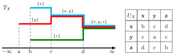
Figure 2: On the left, a treegram $T_{X}$ build over $X=\{x,y,z\}$, where the horizontal axis represents time (traced backwards in the phylogenetic tree setting). On the right, the corresponding symmetric ultranetwork $U_{X}$.

Persistent homology diagrams

As discussed above, the dendrogram is the main model describing the evolution of species in phylogenetics, and it is heavily used in the hierarchical clustering of datasets (viewed as finite metric spaces). Due to their combinatorial nature, dendrograms can neither be directly vectorized nor used in a machine learning pipeline. However, in the case of single-linkage hierarchical clustering there is a process called the Elder-rule which extracts a persistence diagram from the single linkage dendrogram as in [12, Defn. 3.7]. Persistence Diagrams are multisets of points in the extended plane $(\mathbb{R}\cup\{\infty\})^{2}$. The persistence diagram obtained in this way corresponds to the $0$-dimensional persistent homology diagram with respect to the Vietoris-Rips filtration of the dataset. This is a special case of the more broad method of $p$-dimensional persistent homology diagrams of filtrations, which capture the evolution of $p$-dimensional cycles across the filtration of the dataset [15].

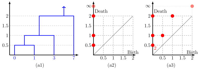
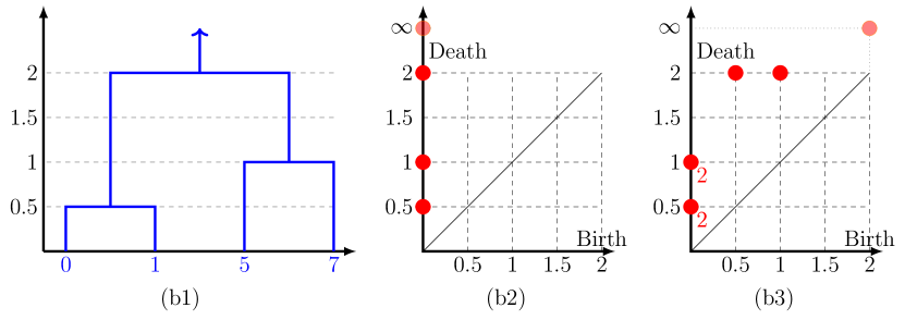
Figure 3: Consider the finite metric subspaces $X=\{0,1,3,7\}$ and $Y=\{0,1,5,7\}$ of $(\mathbb{R},|\cdot|)$. (a1) shows the single-linkage dendrogram of $X$, (a2) shows the $0$-dimensional persistent homology diagram of $X$, and (a3) shows the mergegram of the single-linkage dendrogram of $X$. (b1) shows the single-linkage dendrogram of $Y$, (b2) shows the $0$-dimensional persistent homology diagram of $Y$, and (b3) shows the mergegram of the single-linkage dendrogram of $Y$. The datasets $X$ and $Y$ have the same $0$-dimensional persistent diagrams but different mergegrams.

The mergegram of a dendrogram

Persistent homology diagrams will not always be able to distinguish different metric spaces (see Fig. 3). In [16], the authors considered a new invariant for datasets, called the mergegram. The mergegram is defined for every dendrogram as the multiset of interval lifespans of the blocks of the partitions across the dendrogram (in other words, the multiset of the intervals of all the edges in the underlying tree of the dendrogram); in the case of datasets, the mergegram associated with a dataset is the mergegram of the single linkage dendrogram of the dataset. In particular, the authors showed that the mergegram is stronger invariant than the $0$-dimensional persistent homology diagram of datasets, i.e. if two metric spaces have the same mergegram then they have the same $0$-dimensional persistence diagrams, but not vice versa (see Fig. 3).

By construction of the mergegram, as a multiset of intervals, we can also think of it as a persistence diagram. The mergegram -when viewed as persistence diagram- (i) is stable and at the same time (ii) it is naturally equipped with a family of computable metrics (e.g. Wasserstein and Bottleneck distances) while (iii) still capturing essential information about the dendrograms. Another consequence of viewing mergegrams as persistence diagrams is the possibility of using existing machinery/vectorization of persistence diagrams for a subsequent data analysis pipeline.

Loops in the tree of life

In real world, mutations of genetic sequences are often accompanied by their recombinations. Such joint phenomena are modeled by a phylogenetic network that generalizes the notion of a phylogenetic tree. The most common model for visualizing those networks is that of a rooted directed acyclic graph (rooted DAG), [31]. The recombination events will give rise to loops in the DAG. These DAGs are typically generated from coalescent processes that may arise from optimal merging or fitting together a given set of phylogenetic trees. This process is known as the phylogenetic network reconstruction [31]. L. Nakhleh proposed the following formulation which will be referred to in this paper as the Phylogenetic Network Reconstruction Problem (PNRP), (pg. 130 in [31]): Given a family $\mathcal{F}$ of phylogenetic trees over a common set of taxa $X$, is there a unique minimal phylogenetic network $N$ whose set of spanning trees $\mathcal{T}(N)$ contains the family $\mathcal{F}$? There are different answers to PNRP, due to the different ways of defining what a ‘minimal network’ is (based on different optimization criteria). The existing methods and software use DAG-type models to describe the phylogenetic networks [7, 19, 20, 37, 39].

1.2 Overview of our contributions

In this work, we propose two lattice-theoretic models for phylogenetic reconstruction networks. These approaches have several advantages. Firstly, each of these lattice-models provides us with a unique solution to the PNRP (see Prop. 2.5 and Rem. 2.6). Moreover, our models are constructed using tools from TDA such as networks, filtrations [29], persistence diagrams [10], mergegrams [16], and their associated metrics [4, 10]. In addition, those lattice models provide us with interleaving or Gromov-Hausdorff type of metrics for compairing pairs of phylogenetic trees and networks over different sets of taxa [23]. Below, we give a detailed overview of our results.

Our first order viewpoint on the phylogenetic reconstruction process

In the setting of phylogenetic trees, we cannot model recombination phenomena, that would naturally correspond to a loop in the structure (not present in trees). Hence, the simple model of trees (modeled with dendrograms) should be extended to rooted DAGs with an additional structure allowing to keep track of the evolution of taxa. Such a structure is modeled, in this work, by a cliquegram (see Defn. 2.15) being a nested family of sets of cliques over $X$, as presented in Fig. 4. Note that when the taxa sets decorating the edges of the cliquegram are forgotten, a rooted DAG is recovered.

Figure 4: On the left there is a cliquegram $C_{X}$, on the right - the associated phylogenetic network $N_{X}$.

In the cliquegram, presented in Fig. 4, the time axis is represented by a horizontal line. In order to recover the taxa set of biological entities at the time $t$, a vertical line should be placed at time $t$ and the cliques at the intersection of the structure with that line will indicate the taxa set (a.k.a. taxonomy) of those entities. For instance, for $t\in(c,d)$, we have two entities; the first having a taxa set $\{x,y\}$ and the second having a taxa set $\{y,z\}$. Note that the intersection of their taxonomies, $\{y\}$ (present at times $t<c$), is a common taxon of both entities and creates the loop in the structure. That implies the existence of their common predecessor, whereas the union of their taxonomies, $\{x,y,z\}$ (present at times $t>d$), implies the existence of their common ancestor.

While dendrograms naturally correspond to ultrametrics, cliquegrams also have a corresponding structure as a subclass of symmetric networks, which we call phylogenetic networks (see Defn. 2.8). There is an isomorphism between the lattice $\mathbf{Net}(X)$, of the phylogenetic networks $N_{X}$ over $X$, and the lattice $\mathbf{Cliqgm}(X)$ of all cliquegrams $\mathcal{C}_{X}$ over $X$ explicitly defined in Prop. 2.17. See the right part of the Fig. 4 as an example of the correspondence; Given $a,b\in\{x,y,z\}$, the entry of the matrix at the position $(a,b)$ indicates the time of coalescence of the taxa $a$ and $b$ that can be read out of the cliquegram by taking the time instance when they are merged together.

One of the main observations of this work is that the lattice structure of cliquegrams over $X$, as opposed to ordinary rooted DAGs, enables us to provide a unique answer to the PNRP, meaning that the PNRP has a unique solution in the setting of cliquegrams: Given any family $\mathcal{F}$ of treegrams over the common set of taxa $X$, there exists a unique minimal cliquegram $C_{X}^{(F)}$ (w.r.t. the partial order $\leq$ in the lattice of all cliquegrams over $X$) containing each treegram in $\mathcal{F}$. The cliquegram $C_{X}$ is given explicitly as the join of $\mathcal{F}$, $\vee\mathcal{F}$ (see Rem. 2.6 and Prop. 2.35). See also Fig. 5.

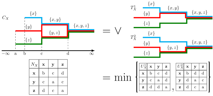
Figure 5: An example of cliquegram $\mathcal{C}_{X}$ over $X$ obtained as the join of two treegrams over $X$. The associated phylogenetic network $N_{X}$ of the cliquegram $\mathcal{C}_{X}$ can be obtained as the pointwise minimum of the associated ultranetworks of the spanning treegrams of $C_{X}$.

This observation allows us to devise a simple algorithm for computing the join cliquegram from any given family of treegrams. The join cliquegram $C_{X}$ of the family $\mathcal{F}$, is then given by the maximal cliques of the Vietoris-Rips complex of $N_{X}$. A Python implementation of this algorithm is provided in [14].

Since the cliquegram is obtained by a phylogenetic network $N_{X}:X\times X\to\mathbb{R}$ which is a weighted graph, and thus a one-dimensional structure, the approach introduced in this section is referred to as first order approach.

Our higher order viewpoint of the phylogenetic reconstruction process

The notion of a phylogenetic network $N_{X}$ (see Defn. 2.8) extends, in a natural way, to the notion of a filtration $F_{X}$ (see Defn. 2.22). In what follows, for the purpose of visualizing the evolution of maximal faces in a filtration, filtrations will be represented as facegrams (see Defn. 2.29) which are structures that generalize cliquegrams and dendrograms (see Rem. 2.28). A facegram encodes the evolution of maximal faces across a filtration of simplicial complexes. In the special case where the filtration is the Vietoris-Rips filtration of a phylogenetic network $N_{X}$ over $X$, the associated facegram is exactly the cliquegram of $N_{X}$.

The process of constructing a facegram from a given filtration turns out to be an equivalence (in particular, a bijection) between filtrations and facegrams, in the following sense: Let $X$ be a set of taxa. There is an isomorphism between the lattice $\mathbf{Filt}(X)$ of all filtrations over $X$ and the lattice $\mathbf{Facegm}(X)$ of all facegrams over $X$. The maps between them are explicitly defined in Prop. 2.31. For an example of the equivalence, consult Fig. 6; on the left, the facegram built on taxa $\{x,y,z\}$. On the right, is the isomorphic filtration.

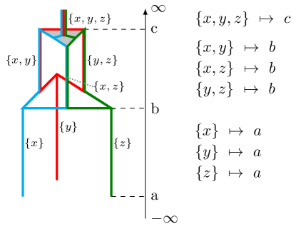
Figure 6: An example of facegram and its associated filtration.

By definition, every cliquegram is a particular type of facegram (see Fig. 10). Hence, in a much broader sense, we can ask whether we can model a more broad phylogenetic reconstruction process as a join operation on the lattice of facegrams, instead of the more restricted setting of the lattice of cliquegrams, see Fig. 7.

Figure 7: Consider the set of three treegrams in the middle of the picture. The structure on the left is obtained by taking the join operation on those treegrams (viewed as cliquegrams) in the lattice of cliquegrams. On the right, the join of the same treegrams (now viewed as facegrams) in the lattice of facegrams is presented. Note that the cliquegram can be obtained from the facegram on the right by squashing the three loops. Hence, sometimes, the facegram contains reticulation loops that are not present in the cliquegram.

It turns out that in this general setting, where treegrams are viewed as facegrams in place of cliquegrams, the following holds:

1. The facegram-join operation yields more information than the cliquegram-join operation, as the cliquegram can be obtained from the facegram (see Fig. 7).

2. In the setting of facegrams, the PNRP still admits a unique solution, in the sense that for any family $\mathcal{F}$ of treegrams (viewed as facegrams) over $X$, there exists a unique minimal facegram $\mathcal{C}_{X}$ (w.r.t. the partial order $\leq$ of facegrams) that contain each treegram in $\mathcal{F}$. Specifically, that facegram $\mathcal{C}_{X}$ is given by the join-span $\vee\mathcal{F}$ (see Prop. 2.32).

Face-Reeb graph and mergegram invariants

The facegram can become very difficult to visualize when the number of taxa is large. Hence, it is important for the applications to study invariants of facegrams that are easy to describe and visualize as well as equipped with a metric structure. This allows comparison of those descriptors (and therefore, indirectly, to allow for comparison of lattice-diagrams) which can be used for statistical inference.

Furthermore, for most machine learning algorithms we need the structure of a Hilbert space and thus a possibility to vectorize the facegram in a sensible way. Due to the weighted-graph nature of the facegram, such a representation should be sensitive to the edges and their weights. For that purpose, we propose two novel topological invariants of facegrams (and thus of filtrations too), (i) the face-Reeb graph of a facegram and (ii) the mergegram of a facegram (by extending a construction by Elkin and Kurlin defined on dendrograms [16]).

We then show the mergegram is a 1-Lipschitz stable invariant, while the face-Reeb graph is not stable. Our main result is that the mergegram is invariant of weak equivalences of filtrations, a stronger form of homotopy equivalence (see Thm. 3.15). The mergegram can be used as a computable proxy for phylogenetic networks and also, more broadly, for filtrations of datasets, which might also be of interest to TDA.

Motivation for introducing cliquegram, facegram and mergegram

In this work, we introduce the cliquegram and the facegram in order to obtain an analogous construction to the dendrogram of an ultrametric for the general case of a phylogenetic network and more broadly to a filtration, respectively. Dendrograms are in one-to-one correspondence with ultrametrics. However, dendrograms are useful (i) for visualizing ultrametrics and (ii) for obtaining invariants from ultrametrics, i.e. (a) the $0$-dimensional sublevel set persistence of a metric space $(X,d_{X})$ can be obtained by applying the Elder rule on the dendrogram of the single linkage ultrametric of $(X,d_{X})$, and (b) the mergegram of a dendrogram [16]. In order to obtain analogous constructions to dendrograms for networks and filtrations, we first observed that partitions are a special case of clique-sets and clique-sets are a special case of face-sets over $X$. Combined with the fact that dendrograms are filtered partitions, the preceding argument motivated us to define cliquegrams as filtered clique-sets and facegrams as filtered face-sets, respectively. Except for generalizing dendrograms, cliquegrams, and facegrams are also useful, since:

1. (Biological motivation) Through those lattices we can model the join-span of a set of treegrams (viewed as cliquegrams or facegrams respectively), and thus obtain a phylogenetic structure that can accommodate loops.

2. (Mathematical motivation) By viewing filtrations as facegrams, we can craft new invariants of filtrations by crafting invariants of facegrams, such as the face-Reeb graph and the mergegram, those are invariants of filtrations which we couldn’t obtain directly from the filtration but only through its facegram.

Computational complexity and experiments

In the last section, we give polynomial upper bounds on the computational complexity of the phylogenetic network reconstruction process that is modeled as the join-facegram of a set of treegrams (see Thm. 4.4). The same complexity upper bound applies when computing the mergegram invariant of the join-facegram. We provide implementations of our algorithms in Python. Next, we apply our algorithms to certain artificial datasets and to a certain benchmark biological dataset.

It should be noted, that most TDA approaches for phylogenetic trees/networks take either the approach of considering vertices as points in high-dimensional space (and use the distance in this space) or use the tree distances directly to construct Vietoris-Rips complexes to capture connected components as well as cycles in the networks for the analysis of the data, see [6, 9]. In this work, on the other hand, a new diagrammatic model is constructed for the phylogenetic tree/networks, and mathematical properties of this representation are established in terms of Nakhleh’s phylogenetic reconstruction problem. Subsequent analysis is done on this model structure.

Appendix

We relegate some of the proofs of the next sections to the appendix.

1.3 Relation of our work with other research works

Relation of facegrams with dendrograms and treegrams

For a given partition $P_{X}$ of set $X$, to every block in the partition corresponds a total complex, and thus, $P_{X}$ gives rise to a simplicial complex, given by the disjoint union of these total complexes. Hence, dendrograms (and treegrams) can be viewed as filtered complexes or equivalently filtrations. The corresponding facegram of that filtered complex is our dendrogram (resp. treegram). However, both the dendrogram and the treegram model do not allow recombinations that would introduce loops to our tree of life.

Relation of facegrams with formigrams

An extension of treegrams which allows for the formation of loops is the formigram [22, 23]. By a formigram over $X$, here we mean a filtered subpartition $S_{X}:\mathbf{Int}\to\mathbf{SubPart(X)}$ over the poset of closed intervals of $\mathbb{R}$, $\mathbf{Int}$. It should be noted that the PNRP also admits a solution in the lattice of formigrams, if we consider the join-operation on a given family of treegrams. However, the join of a set of treegrams (when viewed as formigrams) would still be a treegram, so no recombination events can be recorded/represented in this join-structure. Facegrams, on the other hand, do accommodate recombinations (loops) when realized as joins of treegrams while maintaining an $\mathbb{R}$-filtration model for our tree of life. This point of view provides a generalization of the concept of dendrograms and treegrams that accommodates loops and at the same time it links facegrams to the machinery of filtrations from TDA (i.e. $\mathbb{R}$-filtrations). Finally, we note that although the formigram is not the same as the facegram, these structures are embedded into a common generalized construction: Firstly, we observe that the notion of facegrams indexed over the poset of $\mathbb{R}$, generalizes over an arbitrary poset $\mathbf{P}$. For the case of the poset $\mathbf{P}=\mathbf{Int}$, given that the lattice of face-sets contains the lattice of subpartitions, facegrams over the poset $\mathbf{Int}$, would be a construction that generalizes both the formigram model and our model of facegrams over the poset $\mathbb{R}$.

Relation to join-decompositions of poset maps

In this work, we also utilize the machinery of join-decompositions of order-preserving maps and their associated interleaving distances as developed in [23]. Specifically we consider maps from the poset $(\mathbb{R},\leq)$ to the lattice of face-sets which includes the lattice of subpartitions $\mathbf{SubPart}(X)$ (see Defn. 2.29), and we establish certain decompositions of our structures into indecomposables (see Prop. 2.32, Cor. 2.33 and Prop. 2.35, Cor. 2.36).

Relation of mergegrams with other invariants

Formigrams can be viewed as functors from $\mathbf{Int}$ to $\mathbf{SubPart}$, see [23]. In [21] the authors introduced the maximal group diagram and the persistence clustergram. In our work, we are studying the facegram construction as a functor from $\mathbb{R}$ to $\mathbf{Face}$ (which is different from the formigram functor) and we introduce three invariants of that construction, the face-Reeb graph, the mergegram, and the labeled mergegram. Note that dendrograms (as well as treegrams) can be viewed as facegrams and also as formigrams at the same time. However, even in that case, our invariants are different from the ones used in [21]. Indeed, suppose one has a dendrogram with two leaves $\{x,y\}$ merging at some time instance $t$. Then, the maximal group diagram of the dendrogram will contain three intervals $[0,\infty),[0,\infty),[t,\infty)$, corresponding to $\{x\},\{y\},\{x,y\}$, respectively, the persistent clustergram will contain the three intervals $[0,t),[0,t),[0,\infty)$, corresponding to $\{x\},\{y\},\{x,y\}$, respectively, whereas the labeled mergegram will contain the intervals $[0,t),[0,t),[t\infty)$, corresponding to $\{x\},\{y\},\{x,y\}$, respectively. Although those invariants are different the formalism is quite similar. It seems possible that one can define invariants for facegrams over the poset $\mathbf{Int}$ that may generalize all those invariants, but this topic was out of scope of this paper, so we didn’t develop such ideas further.

2 Diagrammatic models

In this chapter we recall certain results from the theory of lattices [23], then we develop two different lattice-diagram models for visualizing phylogenetic reconstruction networks and more broadly filtrations, the cliquegram and the facegram, respectively, and we show that in each of those settings, the PNRP admits a unique solution. The facegram, except being a model for phylogenetic networks, more broadly, it is also related to the notion of filtered simplicial complexes that are used in applied topology.

2.1 Lattice structures

In this section, we review the basic notions and results of the theory of lattices [17, 33] as well as some results from [23] in order to help us properly formulate the PNRP and explain why it always admits a solution in the lattice setting. Finally, we consider the notion of diagram over a lattice from [23], which we refer to simply as the lattice-diagram.

A lattice $\mathcal{L}=(\mathcal{L},\leq,\vee,\wedge)$ is a poset $(\mathcal{L},\leq)$ (a binary relation $\leq$ on $\mathcal{L}$ which is reflexive, transitive, and antisymmetric) that admits all finite joins $\vee$ and meets $\wedge$. For every $X,Y$ in $\mathcal{L}$, we say that $X$ is a join of $Y$ if $Y=X\vee Z$, for some $Z$ in $\mathcal{L}$. For every $X,Y$ in $\mathcal{L}$, we denote by $[X,Y]:=\{Z\in\mathcal{L}\mid X\leq Z\leq Y\}$. A lattice that admits all joins and meets is called a complete lattice and is denoted by $(\mathcal{L},\leq,\vee,\wedge,0,1)$ (where $0:=\wedge\mathcal{L}$ is the bottom element and $1:=\vee\mathcal{L}$ is the top element). Any finite lattice is complete. A subset $\mathcal{B}\subset\mathcal{L}$ (possibly infinite) of a lattice $\mathcal{L}$ is said to be a join-dense subset of $\mathcal{L}$ if every $X$ in $\mathcal{L}$ is the join of a finite number of elements in $\mathcal{B}$.

Example 2.1.

An element $X$ of $\mathcal{L}$ is join-irreducible if it is not a bottom element, and, whenever $X=Y\vee Z$, then $X=Y$ or $X=Z$. If the lattice $\mathcal{L}$ is finite, then the join-irreducible elements of $\mathcal{L}$ are join-dense.

Proposition 2.2 ([23, Prop 3.2]).

Let $\mathcal{L}$ be a lattice and let $X$ in $\mathcal{L}$. Then, $X=\bigvee(\mathcal{B}\cap[0,X])$.

Definition 2.3.

We will call the (maximal) elements of the set $\mathcal{B}(X):=\mathcal{B}\cap[0,X]$ the (maximal) spanning $\mathcal{B}$-elements of $X$.

Example 2.4.

Let $X$ be a finite set. Let $\mathcal{G}_{X}=(\mathcal{G}_{X},\subset,\cup,\cap)$ be the lattice of all connected simple graphs $(V,E)$ with vertex set $V=X$. Then, the set $\mathcal{T}_{X}$ of all tree graphs with vertex set $X$ is a join-dense subset of $\mathcal{G}_{X}$. In particular, for any given graph $(X,E)$ in $\mathcal{G}_{X}$ the spanning $\mathcal{T}_{X}$-elements of $(X,E)$ are exactly the spanning trees of $(X,E)$.

Proposition 2.5 (Minimal join-reconstruction in a complete lattice setting).

Let $\mathcal{L}=(\mathcal{L},\vee,\wedge,0,1)$ be a complete lattice and let $\mathcal{B}$ be a join-dense subset of $\mathcal{L}$. Any element $X$ in $\mathcal{L}$ is equal to the join $\vee\mathcal{B}(X)$ of its spanning $\mathcal{B}$-elements. In addition, for any family $\mathcal{F}$ of elements in $\mathcal{B}$, there exists a unique $\leq$-minimal element $X$ in $\mathcal{L}$ such that $\mathcal{F}\subset\mathcal{B}(X)$, and moreover, that unique such element $X$ is simply given by the join $\vee\mathcal{F}$.

Proof.

The first part of the proof is equivalent to Prop. 2.2. Now, for the second part, consider

$$X:=\bigwedge\{Y\in\mathcal{L}\mid\mathcal{F}\subset\mathcal{B}(Y)\}.$$

This is the unique $\leq$-minimal element $X$ such that $\mathcal{F}\subset\mathcal{B}(X)$, which exists since the lattice $\mathcal{L}$ is complete. Now, we claim that $X=\vee\mathcal{F}$.

• Note that $X$ is a non-empty meet: for $Y:=\vee\mathcal{F}$, $\mathcal{F}\subset\mathcal{B}(Y)$ since $\mathcal{B}(Y)=\mathcal{B}\cap[0,Y]\supset\mathcal{F}$.

• By the subsequent argument $\vee\mathcal{F}$ lies in the set that meet-spans $X$. Since the meet $X$ is always less or equal to all the elements in that set, then $X\leq\vee\mathcal{F}$.

• We claim that $\vee\mathcal{F}\leq X$: Let $Y\in\mathcal{L}$ such that $\mathcal{F}\subset\mathcal{B}(Y)$ and let $Z\in\mathcal{F}$. It suffices to check that $Z\leq Y$. Indeed, $Z\in\mathcal{F}\Rightarrow Z\in\mathcal{B}(Y)$. Thus, $Z\leq\vee\mathcal{B}(Y)=Y$.

• Finally, by combining all the previous arguments, we obtain that the element $X=\vee F$ is the unique $\leq$-minimal element in $\mathcal{L}$ such that $\mathcal{F}\subset\mathcal{B}(X)$.

∎

Remark 2.6.

If we model properly phylogenetic networks over a fixed finite set of taxa as a finite lattice (and thus complete lattice in particular) and treegrams over that set of taxa as a join-dense subset of that lattice, then by Prop. 2.5 the PNRP will admit a unique solution in this lattice. In the next section we craft two different lattice-diagram models for phylogenetic networks for each of which the collection of all treegrams is the set of join-irreducible elements, and thus in each of these lattice-diagram models, the PNRP admits a solution in particular.

Diagrams over lattices

Let $\mathcal{L}=(\mathcal{L},\vee,\wedge)$ be a finite lattice, which we fix here. An $\leq$-filtered diagram $X^{\bullet}:=\ldots\leq X^{i}\leq X^{i+1}\leq\ldots$ of elements in $\mathcal{L}$ is called a $\mathcal{L}$-diagram. Equivalently, an $\mathcal{L}$-diagram is an order-preserving map of posets $X^{\bullet}:(\mathbb{R},\leq)\to(\mathcal{L},\leq)$. The collection of all $\mathcal{L}$-diagrams forms a lattice on its own. The partial order is given by $X^{\bullet}\leq Y^{\bullet}\Leftrightarrow X^{t}\leq Y^{t}$, for all $t\in\mathbb{R}$.

Example 2.7 (Dendrograms as lattice-diagrams).

Let $X$ be a finite set. A partition of $X$ consists of a collection $P_{X}=\{B_{1},\ldots,B_{n}\}$ of subsets $B_{i}$ of $X$, $i=1,\ldots,n$, called blocks, such that $\cup_{i=1}^{n}B_{i}=X$ and $B_{i}\cap B_{j}=\emptyset$, for all $i\neq j$. Let $\mathbf{Part}(X)$ be the lattice of partitions $P_{X}$ on $X$ where the partial order is give by

$$P_{X}\leq P^{\prime}_{X}\Leftrightarrow\forall S\in P_{X}\text{, }\exists S^{\prime}\in P^{\prime}_{X}\text{, such that }S\subset S^{\prime}.$$

A $\mathbf{Part}(X)$-diagram $P_{X}^{\bullet}:(\mathbb{R},\leq)\to(\mathbf{Part}(X),\leq)$ is the same thing as a dendrogram over $X$.

2.2 The cliquegram of a phylogenetic network

In this section, for a set of taxa $X$, we will start from a phylogenetic network $N_{X}:X\times X\to\mathbb{R}$ (see Defn. 2.8) and then associate to it a lattice-diagram $C_{X}$ using the maximal cliques of the network called the cliquegram of $N_{X}$ (see Defn. 2.15). The assignment $N_{X}\mapsto C_{X}$ lifts to a one-to-one correspondence between phylogenetic networks and cliquegrams, which generalizes the one-to-one correspondence between symmetric ultranetworks and treegrams [36] and the one-to-one correspondence between ultrametrics and dendrograms [8]. Furthermore, we devise an algorithm for reconstructing a cliquegram from a given set of phylogenetic trees. An implementation of this algorithm can be found in [14].

Phylogenetic networks

In the field of mathematical phylogenetics, we are interested in studying evolutionary relationships among biological entities. Each biological entity is called a taxon. The set of all taxa is denoted by $X$ and let us fix it from now on. Relationships among the taxa of $X$ are modeled by a weighted DAG on $X$ called a phylogenetic network. More concretely, a phylogenetic network $N_{X}$ over $X$ can be identified with a real-valued matrix $N_{X}$ over $X$, namely, a map $N_{X}:X\times X\to\mathbb{R}$: By viewing the poset $(\mathbb{R},\leq)$ as time traced backwards, each value $N_{X}(x,x^{\prime})$, $x,x^{\prime}\in X$, of the matrix represents the time, traced backward, when the taxa $x,x^{\prime}$ were mutated from their most recent common ancestor, and it is called time to coalescence of $x$ and $x^{\prime}$. If $x=x^{\prime}$, the interpretation of $N_{X}(x,x)$ is that it is the time, traced backwards, when the taxon $x$ was first observed in the phylogenetic network, called time of observation of $x$. Because of this biological interpretation for $N_{X}$ and the consideration that time is traced backward, for any $x,x^{\prime}$ in $X$:

1. The matrix $N_{X}$ must be symmetric in $x,x^{\prime}$

2. The time $N_{X}(x,x)$ of observation of $x$ and the time $N_{X}(x^{\prime},x^{\prime})$ of observation of $x^{\prime}$ must be less or equal to the time $N_{X}(x,x^{\prime})$ to coalescence of $x$ and $x^{\prime}$.

Definition 2.8.

A phylogenetic network over $X$ is a map $N_{X}:X\times X\to\mathbb{R}$ such that

1. $N_{X}(x,x^{\prime})=N_{X}(x^{\prime},x)$, for all $x,x^{\prime}\in X$,

2. $\max\{N_{X}(x,x),N_{X}(x^{\prime},x^{\prime})\}\leq N_{X}(x,x^{\prime})$, for all $x,x^{\prime}\in X$.

We denote by $\mathbf{Net}(X)$ the lattice of all phylogenetic networks over $X$, whose partial order, meets and joins are given by entry-wise reverse inequalities, maximums, and minimums, respectively.

Example 2.9.

Let $X$ be a set of taxa. A matrix $D_{X}:X\times X\to\mathbb{R}$ such that for all $x,x^{\prime},x^{\prime\prime}\in X$:

1. $D_{X}(x,x^{\prime})=D_{X}(x^{\prime},x)$,

2. $D_{X}(x,x^{\prime\prime})\leq D_{X}(x,x^{\prime})+D_{X}(x^{\prime},x^{\prime\prime})$,

3. $D_{X}(x,x^{\prime})\geq 0$,

4. $D_{X}(x,x^{\prime})=0\Leftrightarrow x=x^{\prime}$,

is said to be a metric. If the matrix is satisfying only the first three, then it is called a pseudometric. If $D_{X}$ satisfies the first condition and also $D_{X}(x,x^{\prime\prime})\leq\max\{D_{X}(x,x^{\prime}),D_{X}(x^{\prime},x^{\prime\prime})\}$, then $D_{X}$ is said to be a symmetric ultranetwork [36]. If it is also a metric, then it is called an ultrametric. We easily check that in all cases the matrices satisfy the two axioms of a phylogenetic network. From now on, we will also call any symmetric ultranetwork a phylogenetic tree.

We are now investigating a lattice-diagram representation for phylogenetic networks, visualized by a certain DAG, which generalizes the treegram representation of symmetric ultranetworks; a richer structure that allows for undirected loops in that DAG.

Recall that a treegram consists of an increasing sequence of subpartitions of $X$. Now, to allow our representation to have loops we introduce a generalization of the notion of subpartition of a set $X$, i.e. a family of ‘blocks’ (subsets) of $X$, such that

1. At each level, each block is maximal in the sense that no block is contained in another block.

2. Intersections between the blocks of $X$ are allowed so that loops can be formed in the network, as time is traced backward.

If we think of a subpartition of $X$ as an equivalence relation $R$ on a subset $X_{R}$ of $X$, then condition 2. above, simply proposes dropping the ”transitivity property” on $R$, and thus it prompts for considering only symmetric and reflexive relations $R$ on the subset $X_{R}$ of $X$ (not necessarily transitive). A symmetric and reflexive relation $R$ on $X_{R}\subset X$ is simply a graph $G_{R}$ on the vertex subset $X_{R}$ of $X$. An analog of a ‘block’ in the setting of graphs, is a maximal connected subgraph $B$ of the graph $G_{R}$, called a maximal clique of a graph .

Below, we provide an abstract notion of a set $\mathcal{S}$ of cliques of $X$, without a reference to a graph.

Definition 2.10.

A clique-set of $X$ is a set $\mathcal{C}_{X}$ of subsets of $X$, called cliques, such that

1. no subset in $\mathcal{C}_{X}$ is contained in another subset in $\mathcal{C}_{X}$, and

2. every set $X$ of vertices in which all pairs are contained in some clique in $\mathcal{C}_{X}$ is also contained in a clique in $\mathcal{C}_{X}$, i.e. : for any $Y\subset X$, if for any $y,y^{\prime}\in Y$, there exists $C_{y,y^{\prime}}\in\mathcal{C}_{X}$ such that $\{y,y^{\prime}\}\subset C_{y,y^{\prime}}$, then $Y\subset C$, for some $C\in\mathcal{C}_{X}$.

We denote by $\mathbf{Cliq}(X)$ the lattice of all clique-sets over $X$, whose partial order is given by $\mathcal{C}_{X}\leq\mathcal{C}^{\prime}_{X}$ if and only if, for any clique $C\in\mathcal{C}_{X}$, there exists a clique $C^{\prime}\in\mathcal{C}^{\prime}_{X}$ such that $C\subset C^{\prime}$.

Example 2.11.

Below, we give some examples of clique-sets.

• If $G_{X}$ is a graph over $X$, then the set $C_{X}$ of all maximal cliques of $G_{X}$ is a clique-set of $X$.

• A partition $P_{X}=\{B_{1},\ldots,B_{n}\}$ of $X$ is a clique-set over $X$.

• A collection $P_{X}=\{B_{1},\ldots,B_{n}\}$ of pairwise disjoint subsets of $X$ (not necessarily covering all of $X$), called a subpartition of $X$ [22, 36], is a clique-set over $X$.

Remark 2.12.

Note that the maximal cliques of a graph give rise to a natural one-to-one correspondence between graphs and clique-sets. See Prop. A.1 in Appendix.

Cliquegrams

We show that a phylogenetic network can be represented by a diagram of clique-sets, called the cliquegram (a portmanteau of ‘clique-set-diagram’), a representation which generalizes the treegram representation of symmetric ultranetworks [36]. Let $N_{X}$ be a phylogenetic network over a set of taxa $X$. For any $t\in\mathbb{R}$, we can define a graph $G_{t}^{X}=(V_{t}^{X},E_{t}^{X})$, given by

• $V_{t}^{X}:=\{x\in X\mid N_{X}(x,x)\leq t\}$,

• $E_{t}^{X}:=\left\{\{x,x^{\prime}\}\subset X\mid N_{X}(x,x^{\prime})\leq t\text{ and }x\neq x^{\prime}\right\}.$

Remark 2.13.

Note that the graph $G_{t}^{X}=(V_{t}^{X},E_{t}^{X})$ is well-defined since $N_{X}$ satisfies the second assumption in Defn. 2.8. $G_{t}^{X}$ is well-defined only for phylogenetic networks. Indeed, if $N_{X}$ is not a phylogenetic network, but rather, a symmetric network that does not satisfy the second assumption in Defn. 2.8, then $G_{t}^{X}$ will contain an edge that does not contain both of its incident vertices.

Let $\mathcal{C}_{X}(t)$ denote the set of all maximal cliques of $G_{t}^{X}$. We call the map $\mathcal{C}_{X}:\mathbb{R}\to\mathbf{Cliq}(X)$, $t\mapsto\mathcal{C}_{X}(t)$, the cliquegram representation of $N_{X}$. It is easy to check that (i) $\mathcal{C}_{X}$ forms as order-preserving map $\mathcal{C}_{X}:(\mathbb{R},\leq)\to\mathbf{Cliq}(X)$, and (ii) there exists a $t_{0}\in\mathbb{R}$ such that $\mathcal{C}_{X}(t)=\{\{X\}\}$, for $t\geq t_{0}$, and $\mathcal{C}_{X}(t)=\emptyset$, for $t\leq-t_{0}$.

Remark 2.14.

Note that, if $N_{X}$ is a metric space, then for any time $t\in\mathbb{R}$, the clique-set $\mathcal{C}_{X}(t)$ is equal to the set of all maximal simplices of the Vietoris-Rips complex of $N_{X}$ at time $t$. Also, note that if $N_{X}$ is a symmetric ultranetwork or an ultrametric, then the associated cliquegram $\mathcal{C}_{X}$ would be a treegram or a dendrogram, respectively.

Hence, the cliquegram representation of phylogenetic networks generalizes the treegram representation of a symmetric ultranetwork [36] and the dendrogram representation of an ultrametric [8], respectively.

Algorithm 1 The cliquegram of a phylogenetic network

1:Input: A phylogenetic network $N_{X}$. Order all the different values of the coefficients $N_{X}(x,x^{\prime})$ of the distance matrix in an increasing way. Let $M$ be that ordered set of real numbers.

2:$L\leftarrow\emptyset$

3:for all $\epsilon\in M$ taken in an increasing order do

4:     $G_{i}$ $\leftarrow$ Build the graph $G_{i}$ with vertex set $V(G_{i}):=X$

5: $G_{i}$ $\leftarrow$ and edge-set $E(G_{i}):=\left\{(x,x^{\prime})\in X\times X\mid N_{X}(x,x^{\prime})\leq\varepsilon\right\}.$

6:     $L\leftarrow L\cup\{\epsilon,$ maximal cliques of $G_{i}\}$

7:end for

8:Return $L$ (A nested sequence of clique-sets of $X$, i.e. the cliquegram associated to $D$.)

An implementation can be found in [14]. Next, we give an abstract notion of a cliquegram without a reference to a phylogenetic network.

Definition 2.15.

Let $X$ be a finite set of taxa.

• A cliquegram over $X$ is a map $\mathcal{C}_{X}:\mathbb{R}\to\mathbf{Cliq}(X)$, such that:

  1. $\mathcal{C}_{X}(t)\leq\mathcal{C}_{X}(s)$, for all $t\leq s$ (where $\leq$ denotes ‘refinement’ of clique-sets),

  2. there exists a $t_{0},t_{1}\in\mathbb{R}$, such that $\mathcal{C}_{X}(t)=\{X\}$, for $t\geq t_{0}$, and $\mathcal{C}_{X}(t)=\emptyset$, for $t\leq t_{1}$,

  3. there exists an ordered set of non-negative real numbers $(\varepsilon_{1}<\ldots<\varepsilon_{s})$, called a critical set, such that $\mathcal{C}_{X}(t)=\mathcal{C}_{X}(s)$, for all $\varepsilon_{i}\leq t<s<\varepsilon_{i+1}$, $i=1,\ldots,s$.

• We denote by $\mathbf{Cliqgm}(X)$ the lattice of all cliquegrams over $X$, whose partial order, meets and joins are given by point-wise inequalities, meets, and joins, respectively.

Remark 2.16.

By definition, the cliquegram can be visualized by a rooted DAG, as in Fig. 8.

The cliquegram representation of phylogenetic networks yields an equivalence between cliquegrams and phylogenetic networks. See Fig. 8. This equivalence guarantees that all the information encoded in the phylogenetic networks is also encoded in the cliquegram and vice versa.

Proposition 2.17.

Let $X$ be a set of taxa. There is an isomorphism

$$\mathbf{Net}(X)\stackrel{{\scriptstyle[}}{{\Psi}}]{\Phi}{\rightleftarrows}\mathbf{Cliqgm}(X)$$

between the lattice $\mathbf{Net}(X)$ of all phylogenetic networks over $X$ and the lattice $\mathbf{Cliqgm}(X)$ of all cliquegrams over $X$. The isomorphism maps $\Phi,\Psi$ are defined as follows

• For any phylogenetic network $N_{X}$, the cliquegram $\Phi(N_{X})$ over $X$ is given for any $t\in\mathbb{R}$ by

  $$\Phi(N_{X})(t):=\bigvee\left\{\{x,x^{\prime}\}\subset X\mid N_{X}(x,x^{\prime})\leq t\right\}.$$

• For any cliquegram $C_{X}$, the phylogenetic network $\Psi(C_{X})$ is given for any $x,x^{\prime}\in X$ by

  $$\Psi(C_{X})(x,x^{\prime}):=\min\{t\in\mathbb{R}\mid x,x^{\prime}\text{ belong to some clique in }C_{X}(t)\}.$$

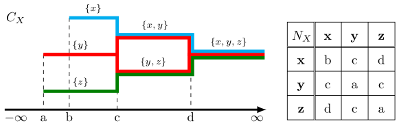
Figure 8: On the left there is a cliquegram $C_{X}$, on the right is the associated phylogenetic network $N_{X}$.

By definition of a cliquegram and Ex. 2.11, it is easy to check that any treegram is also a cliquegram. However, the converse is not true. Thus, Prop. 2.17 can be viewed as a generalization of the equivalence of dendrograms with ultrametrics [8], and of treegrams with symmetric ultranetworks (symmetric ultranetworks) [36].

Remark 2.18.

The biological interpretation of Prop. 2.17 is that there is a phylogenetic network reconstruction process which can be modelled as a lattice-join operation $\vee$ on the collection of cliquegrams over $X$, i.e. any family $\mathcal{F}$ of treegrams will span a unique minimal cliquegram, given by the join-span $\vee\mathcal{F}$.

Remark 2.19.

It is interesting to note that because of Prop. 2.17 and the algebraic viewpoint of the minimum operation on $\mathbb{R}$ as a tropical addition on $\mathbb{R}$ (and therefore the entry-wise minimum of matrices), we can realize the join-cliquegram as a tropical addition on treegrams. We recommend [28] for a thorough introduction to tropical geometry.

Remark 2.20 (Computing the join-cliquegram of a set of treegrams).

Given a set $F$ of treegrams, we can compute the join-cliquegram of $F$ by (i) first computing the minimizer matrix of the associated symmetric ultranetworks of the trees in $F$ (this is the entry-wise minimum of these matrices) and then (ii) taking the associated cliquegram of the network, following Alg. 1.

2.3 The facegram of a filtration

In this section, we define a higher order generalization of a phylogenetic network, called a filtration, which is originated in TDA [29]. We associate a graphical/DAG representation for a filtration, called a facegram, which generalizes the cliquegram representation of a phylogenetic network (see Rem. 2.28 ).

Filtrations

Let $X$ be a set of taxa. Phylogenetic networks $N_{X}$ over $X$ are normally considered modeling evolutionary relationships among taxa, by assigning a certain time instance $N_{X}(x,x^{\prime})$ to each pair $\{x,x^{\prime}\}$ of taxa in $X$, called time to coalescence, if $x\neq x^{\prime}$, and time to observation, if $x=x^{\prime}$. From a combinatorial (topological) viewpoint, perhaps a more natural extension of these coalescence times to a higher order is the following: Let $S=\{x_{1},\ldots,x_{n}\}$ be a subset of $X$. Consider a function $F_{X}:\mathbf{pow}(X)\to\mathbb{R}$ representing for any $S\subset X$ the time $F_{X}(S)$ to coalescence of all the taxa in $S$, where $\mathbf{pow}(X)$ is the set of all non-empty subsets of $X$.

By viewing $(\mathbb{R},\leq)$ as time traced backward, each value $F_{X}(S)$, $S\in\mathbf{pow}(X)$, represents the time, traced backward, when the taxa $S\subset X$ were mutated from their most recent common ancestor. Because of this biological interpretation for $F_{X}:\mathbf{pow}(X)\to\mathbb{R}$ and the consideration that time is traced backwards, for any $S\subset T\subset X$: the time to coalescence of $S$ must be less or equal than the time to coalescence of $T$, i.e. $F_{X}(S)\leq F_{X}(T)$.

Definition 2.21 ([29, Sec. 3]).

Let $X$ be a set of taxa.

• A filtration over $X$ is an order-preserving map $F_{X}:(\mathbf{pow}(X),\subset)\to(\mathbb{R},\leq)$ of posets.

• We denote by $\mathbf{Filt}(X)$ the lattice of filtrations, whose partial order, meets and joins are given by point-wise reverse inequalities, minimums and maximums, respectively.

Below is an example of a filtration, which is given by extending the pairwise-defined time to coalescence model from the setting of phylogenetic networks to the setting of filtrations.

Definition 2.22.

Let $N_{X}:X\times X\to\mathbb{R}$ be a phylogenetic network over a set of taxa $X$. We define the Vietoris-Rips or diameter filtration $\mathbf{VR}_{X}:\mathbf{pow}(X)\to\mathbb{R}$ of $N_{X}$ element-wisely for each $\sigma\in\mathbf{pow}(X)$, as follows:

$$\mathbf{VR}_{X}(\sigma):=\max_{x,x^{\prime}\in\sigma}N_{X}(x,x^{\prime}).$$

By definition, the map $N_{X}\mapsto\mathbf{VR}_{X}$ is injective.

We call the diameter filtration $\mathbf{VR}_{X}$ of a symmetric ultranetwork $U_{X}$, a tree filtration.

Remark 2.23.

The lattice $\mathbf{Net}(X)$ embeds into the lattice $\mathbf{Filt}(X)$ via the Vietoris-Rips filtration construction. Thinking of phylogenetic networks as weighted or filtered graphs, and thus one-dimensional structures, and filtrations as filtered simplicial complexes, then a filtration can be seen as a higher order generalization of phylogenetic networks.

Facegrams

Now, we want to devise a representation for phylogenetic filtrations which (i) generalizes the cliquegram representation of phylogenetic networks and (ii) that can be used for modeling the phylogenetic filtration reconstruction from a given family of phylogenetic trees, if they are viewed as filtrations. From the mathematical-biology point of view, the join-operation on filtrations is expected to be a much richer structure, capturing more reticulations/recombination cycles, than the join-operation on phylogenetic networks. This would be more clear in Ex. 10. To achieve that, we consider a generalization of a clique-set of a set $X$, simply by dropping the second restriction in the definition of a clique-set. First, let’s recall the notion of a simplicial complex.

Definition 2.24.

Let $X$ be a set of taxa. A simplicial complex over $X$ is a collection $S_{X}\subset\mathbf{pow}(X)$ of subsets of $X$, called simplices or faces, which is closed under taking subsets.

By definition, a simplicial set over $X$, $S_{X}$, is a downset in the lattice $(\mathbf{pow}(X),\subset,\cup,\cap)$ of non-empty subsets of $X$. Every finite downset of a given poset is completely determined by its maximal elements. In the case of a simplicial complex $S_{X}$, those are the maximal faces of $S_{X}$.

Definition 2.25.

Let $X$ be a set of taxa.

• A face-set of $X$ is a family $\mathcal{S}_{X}$ of subsets of $X$ that are pairwise incomparable with respect to the inclusion of sets. The elements of a face-set are called faces.

• We denote by $\mathbf{Face}(X)$ the lattice of face-sets of $X$, whose inequalities are given by: $\mathcal{S}_{X}\leq\mathcal{S}^{\prime}_{X}$ if and only if, for any face $C\in\mathcal{S}_{X}$, there exists a face $C^{\prime}\in\mathcal{S}^{\prime}_{X}$ such that $C\subset C^{\prime}$.

Example 2.26.

If $S_{X}$ is a simplicial complex over $X$, then the set $C_{X}$ of all maximal faces $\sigma$ of $S_{X}$ forms a face-set of $X$.

Remark 2.27.

Note that the maximal faces of a simplicial complex give rise to a natural one-to-one correspondence between simplicial complexes and face-sets. See Prop. A.2 in Appendix. In addition, because of that equivalence, the join $C_{X}\vee C^{\prime}_{X}$ of a pair of face-sets of $X$ is equal to the set of maximal faces of the union simplicial complex $S_{X}\cup S^{\prime}_{X}$ of the simplicial complexes $S_{X}$ and $S^{\prime}_{X}$ associated to the face-sets $C_{X}$ and $C^{\prime}_{X}$, respectively.

Let $F_{X}$ be a filtration over a set of taxa $X$. For any $t\in\mathbb{R}$, we define the simplicial complex $S_{X}(t)$, given by

$$S_{X}(t):=\{\sigma\in\mathbf{pow}(X)\mid F_{X}(\sigma)\leq t\}.$$

Let $C_{X}(t)$ denote the face-set of all maximal faces of $S_{X}(t)$. We call the map $C_{X}:\mathbb{R}\to\mathbf{Face}(X)$, $t\mapsto C_{X}(t)$ the facegram representation of $F_{X}$. It is easy to check that (i) $C_{X}$ forms an order-preserving map $C_{X}:\mathbb{R}\to\mathbf{Face}(X)$, and (ii) there exists a $t_{0}\in\mathbb{R}$ such that $C_{X}(t)=\{X\}$, for any $t\geq t_{0}$.

Remark 2.28.

Let $N_{X}$ be a phylogenetic network and let $\mathbf{VR}_{X}:\mathbf{pow}(X)\to\mathbb{R}$ be its associated Vietoris-Rips filtration. Then, the facegram representation $C_{X}$ of the filtration $\mathbf{VR}_{X}$ coincides with the cliquegram representation of $N_{X}$. Therefore, the facegram representation of a filtration is a generalization of the cliquegram representation of a phylogenetic network.

Below, we define the abstract notion of a facegram over $X$ without a reference to a filtration.

Definition 2.29.

Let $X$ be a finite set of taxa.

• A facegram over $X$ is a map $C_{X}:\mathbb{R}\to\mathbf{Face}(X)$, such that:

  1. $C_{X}(t)\leq C_{X}(s)$, for all $t\leq s$ (where $\leq$ denotes ‘refinement’ of face-sets),

  2. there exists a $t_{0}\in\mathbb{R}$, such that $C_{X}(t)=\{X\}$, for any $t\geq t_{0}$, and

  3. there exists an ordered set of non-negative real numbers $(a_{1}<\ldots<a_{n})$, called a critical set, such that $C_{X}(t)=C_{X}(s)$, for all $a_{i}\leq t<s<a_{i+1}$, $i=1,\ldots,n$.

• We denote by $\mathbf{Facegm}(X)$ the lattice of all facegrams over $X$, whose partial order, meets and joins are given by point-wise inequalities, meets, and joins, respectively.

Remark 2.30.

By definition, the facegram can be visualized by a rooted DAG, as in Fig. 9.

Figure 9: An example of a facegram and its associated filtration.

We show that facegrams and filtrations are naturally equivalent (for the proof, see Prop. 2.31).

Proposition 2.31.

Let $X$ be a set of taxa. There is an isomorphism

$$\mathbf{Filt}(X)\stackrel{{\scriptstyle[}}{{\Psi}}]{\Phi}{\rightleftarrows}\mathbf{Facegm}(X)$$

between the lattice $\mathbf{Filt}(X)$ of all filtrations over $X$ and the lattice $\mathbf{Facegm}(X)$ of all facegrams over $X$, where the maps are defined as follows

• For any filtration $F_{X}$, the facegram $\Phi(F_{X})$ over $X$ is given for any $t\in\mathbb{R}$ by

  $$\Phi(F_{X})(t):=\bigvee\left\{S\subset X\mid F_{X}(S)\leq t\right\}.$$

• For any facegram $C_{X}$, the filtration $\Psi(C_{X})$ is given for any $S\subset X$ by

  $$\Psi(C_{X})(S):=\min\{t\in\mathbb{R}\mid S\text{ is contained in some face in }C_{X}(t)\}.$$

Note also that treegrams over $X$ are special cases of facegrams over $X$. In fact, we have the following characterization of treegrams inside the lattice of facegrams.

Proposition 2.32.

A facegram over $X$ is join-irreducible if and only if it is a treegram over $X$. In particular, treegrams are join-dense in the lattice of facegrams. By Rem. 2.6, if we use the facegram as a model of phylogenetic reconstruction, then in this setting the PNRP will admit a solution.

Proof.

($\Leftarrow$) Because in every treegram over $X$ all the taxa in the end are joined to form a single block, each $x\in X$ appears as a leaf in the treegram, so we can restrict to dendrograms. Our claim is equivalent to check that dendrograms over $X$ are join-irreducible in the sublattice of face sets with vertex set exactly equal to $X$: Let $C_{X}$ be a dendrogram, i.e. $C_{X}:(\mathbb{R},\leq)\to\mathbf{Part}(X)$. To show that claim above, it suffices to check it pointwisely. Indeed, at each time $t\in\mathbb{R}$, the face-set $C_{X}(t)$ is a partition of $X$ and thus a face-set of vertex set equal to $X$. If the face-set is not join-irreducible in the lattice of face-sets with vertex set $X$, there would be two other face-sets $C^{\prime}_{X},C^{\prime\prime}_{X}$ such that $C_{X}(t)=C^{\prime}_{X}(t)\vee C^{\prime\prime}_{X}(t)$ with $C^{\prime}_{X}(t),C^{\prime\prime}_{X}(t)\neq C_{X}(t)$, and each with vertex set equal to $X$. Since $C_{X}(t)$ is a partition of $X$, then each of those face-sets should also be a strict partition refinement of $C_{X}(t)$ with the same vertex set $X$. That means that if $S_{X},S^{\prime}_{X},S^{\prime}_{X}$ are the simplicial complexes generated by those face-sets, respectively, then $S_{X}=S^{\prime}_{X}\cup S^{\prime\prime}_{X}$ while both $S^{\prime}_{X},S^{\prime\prime}_{X}$ would be strict subcomplexes of $S_{X}$. So, the maximal faces of $S^{\prime}_{X}$ and the ones for $S^{\prime\prime}_{X}$ are strictly contained in the maximal faces of their union $S_{X}$, and so is their union. That implies that $S^{\prime}_{X}\cup S^{\prime\prime}_{X}$ is strict subcomplex of $S_{X}$, which is clearly a contradiction. Hence, the partition $C_{X}(t)$, viewed as a face-set with vertex set $X$ is indeed join-irreducible in the lattice of face-sets with vertex set equal to $X$.

($\Rightarrow$) If $C_{X}$ is join-irreducible and $C_{X}$ is not a treegram, then there is a minimum value $t_{1}\in\mathbb{R}$ such that the clique-set $C_{X}(t_{1})$ is not a subpartition. However, $C_{X}(t_{1})$ would be a union of finitely many subpartitions. Pick any of them, denoted by $S_{X}(t_{1})$, and then observe that as $t>t_{1}$ the blocks of that subpartition are merged more and more together, creating at times $t>t_{1}$ other (perhaps more than one) choices of subpartitions $S_{X}(t)$ that are coarser than $S_{X}(t_{1})$ until they become a single block $\{X\}$. For each time instance, we make a choice of such a subpartition $S_{X}(t)$. By definition of $t_{1}$, for $t<t_{1}$ $C_{X}(t)=:S_{X}(t)$ was a subpartition of $X$, and thus the map $S_{X}:t\mapsto S_{X}(t)$ is a treegram. Moreover, by definition, the join of all those treegrams $S_{X}$ that are constructed is equal to $C_{X}$ (where they are finitely many of them since $X$ is finite), and thus (i) $C_{X}$ is a finite join of at least two treegrams and (ii) each of those treegrams is different than $C_{X}$, where both (i) and (ii) follow by the assumption that $C_{X}$ itself is not a treegram. Hence, $C_{X}$ is join-reducible, a contradiction.

Lastly, note that treegrams are also join-dense in the lattice of facegrams. Indeed, if $C_{X}$ is a facegram, then there would be a finite set $S$ of critical points. If we take the sublattice of facegram with the same critical set $S$, then since $X$ is finite too, that sublattice would be finite, thus the facegrams would be equal to a join-span of join-irreducible, i.e. treegrams (see Ex. 2.1). ∎

In addition, we obtain the following interesting decomposition, connecting filtrations with tree filtrations $T_{X}$, i.e. the Vietoris-Rips filtrations of symmetric ultranetworks $U_{X}$.

Corollary 2.33.

Let $F_{X}:\mathbf{pow}(X)\to\mathbb{R}$ be a filtration. Because of Prop. 2.32 and Defn. 2.3, $F_{X}$ admits the following decomposition into spanning tree filtrations, i.e.:

$$F_{X}=\min_{T_{X}\geq F_{X}}T_{X}.$$

This decomposition is not unique, since in the above decomposition of $N_{X}$, one can only consider the $\vee$-maximal spanning elements (tree filtrations $T_{X}$) of $N_{X}$ in the lattice of filtrations $(\mathbf{Filt}(X),\geq,\min,\max)$.

Remark 2.34.

Any cliquegram is a facegram, but not vice versa. In addition, there is a surjective lattice morphism from facegrams to cliquegrams: for any given facegram $C_{X}:(\mathbb{R},\leq)\to\mathbf{Face}(X)$ we can construct a cliquegram $C^{\prime}_{X}:(\mathbb{R},\leq)\to\mathbf{Cliq}(X)$ as follows: for each $t\in\mathbb{R}$, we define the $C^{\prime}_{X}(t)$ to be the set of maximal cliques of the $1$-dimensional skeleton (underlying graph) of the simplicial complex generated by the face-set $C_{X}(t)$. See Fig. 10.

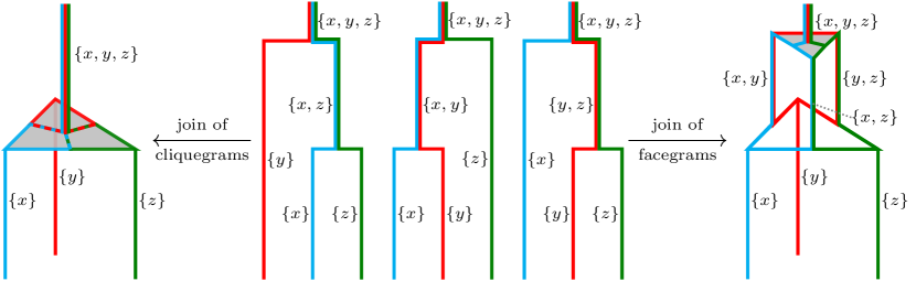
Figure 10: The left shows the join operation on cliquegrams. On the right, there is the join operation on the richer structure of facegrams. The cliquegram can be obtained by the facegram by squashing the three loops. So, the facegram contains reticulation cycles that are not seen by the cliquegram.

We also obtain the following results on cliquegrams.

Proposition 2.35.

Treegrams $C_{X}$ may not be join-irreducible in the lattice of cliquegrams. However, treegrams are join-dense in the lattice of cliquegrams. Thus, by Rem. 2.6 if we use the cliquegram as a model of phylogenetic networks, the PNRP still admits a solution in this setting.

Proof.

Firstly, to see why treegrams may not be join-irreducible, it suffices to restrict to the static (non-filtered) case of clique-sets. The partition $\{\{x,y,z\}\}$ of $X=\{x,y,z\}$ is a clique-set which is not join-irreducible because one has

$$\{\{x,y,z\}\}=\{\{x,y\},\{z\}\}\vee\{\{y,z\},\{x\}\}\vee\{\{z,x\},\{y\}\}.$$

See also Fig. 10.

Next, we show that treegrams are join-dense inside the lattice of cliquegrams: Let $C_{X}$ be a cliquegram and let $S$ be the critical set of $C_{X}$ (the finite set of all time instances $t$ where the clique-sets $C_{X}(t)$ change through time). Now, think of the cliquegram as a facegram. Consider the sublattice of facegrams with critical set $S$. Then, this sublattice is finite (since $S$ and $X$ are finite). Thus, as we have seen in Ex. 2.1, the facegram $C_{X}$ can be written as a join-span of some join-irreducible elements. By Prop. 2.32, those are treegrams. Then, we apply the surjective lattice morphism in Rem. 2.34 from the lattice of facegrams to the lattice of cliquegrams. Since this is a lattice morphism it respects the joinands (the treegrams), and hence, we can write the cliquegram as a join-span of treegrams inside the lattice of cliquegrams now. That means treegrams are join-dense inside the lattice of cliquegrams (although not join-irreducible). ∎

Corollary 2.36.

Symmetric ultranetworks over $X$ are exactly the join-irreducible elements of the lattice of phylogenetic networks over $X$, $\mathbf{Net}(X)$. In particular, in the setting of $\mathbf{Net}(X)$, PNRP admits a solution.

In addition, we obtain the following interesting decomposition, connecting phylogenetic networks (including the case of finite metric spaces) with symmetric ultranetworks.

Corollary 2.37.

Let $N_{X}:X\times X\to\mathbb{R}$ be a phylogenetic network (e.g. a finite metric space). Because of Prop. 2.35 and Defn. 2.3, $N_{X}$ admits the following decomposition into spanning symmetric ultranetworks, i.e.:

$$N_{X}=\min_{U_{X}\geq N_{X}}U_{X}.$$

This decomposition is not unique, since in the above decomposition of $N_{X}$, one can only consider the $\vee$-maximal spanning elements (symmetric ultranetworks $U_{X}$) of $N_{X}$ in the lattice of phylogenetic networks $(\mathbf{Net}(X),\geq,\min,\max)$.

2.4 Metrics for filtrations and facegrams

For facegrams over the same taxa set $X$ we define the interleaving metric between pairs of facegrams over $X$ and we show that it is isometric to the interleaving metric of their associated filtrations. We recall the notion of topological equivalence, weak equivalence, and homotopy equivalence of filtrations over different vertex sets as in [23, 29]. Then, we define the corresponding metrics for comparison of filtrations up to these three types of equivalences. Because of the isometry between interleaving metrics of filtrations and facegrams, and because of the natural equivalence between filtrations and facegrams, the corresponding metrics for comparison of facegrams up to equivalence and up to homotopy equivalence are omitted, since we will not need them: it suffices to focus on metrics on filtrations since all the results about the metrics on filtrations can be transferred to these metrics too.

Metrics for filtrations and facegrams over the same vertex sets

First, we define the interleaving metrics for comparing a pair of filtrations, and facegrams, respectively.

Definition 2.38.

Let $F_{X},F^{\prime}_{X}:\mathbf{pow}(X)\to\mathbb{R}$ be two filtrations over $X$ and let $C_{X},C^{\prime}_{X}:\mathbb{R}\to\mathbf{Face}(X)$ be two facegrams over $X$. We consider the following interleaving distances:

$$d_{\mathrm{I}}(C_{X},C^{\prime}_{X}):=\inf\{\varepsilon\geq 0\mid C_{X}(t)\leq C^{\prime}_{X}(t+\varepsilon)\text{ and }C^{\prime}_{X}(t)\leq C_{X}(t+\varepsilon),\text{ for all }t\in\mathbb{R}\}$$

$$d_{\mathrm{I}}(F_{X},F^{\prime}_{X}):=\max_{\emptyset\neq\sigma\subset X}|F_{X}(\sigma)-F^{\prime}_{X}(\sigma)|$$

Proposition 2.39.

Let $F_{X},F^{\prime}_{X}$ be two filtrations over $X$, and let $C_{X},C^{\prime}_{X}$ be the corresponding facegrams over $X$. Then we have the following interleaving isometry:

$$d_{\mathrm{I}}(C_{X},C^{\prime}_{X})=d_{\mathrm{I}}(F_{X},F^{\prime}_{X}).$$

Proof.

By viewing facegrams equivalently as filtered simplicial complexes, then the proof follows the same way as in the proof of Thm. 4.8 in [23]. ∎

Metrics for filtrations and facegrams over different vertex sets

Quite often in applications of topology, we are interested in studying topological features of filtrations that remain invariant under a weaker notion of equivalence than just a topological equivalence. Such a notion is a weak equivalence of filtrations (also called pullbacks [29]), which is a special type of filtered homotopy equivalence yielded by the pullbacks of a given pair of filtrations (the name pullback appears in [29, Sec. 4.1] and later the name weak equivalence appears in [34, Sec. 6.8]).

Definition 2.40.

Let $X$ and $Y$ be sets. Let $C_{X}$ and $C_{Y}$ be facegrams over $X$ and $Y$, respectively, and let $F_{X},F_{Y}$ be filtrations over $X$ and $Y$, respectively. Then we define the following notions of similarity:

• The facegrams $C_{X},C_{Y}$ are said to be isomorphic if there exists a bijection $\varphi:X\to Y$ such that $C_{Y}(t)=\{\varphi(\sigma)\mid\sigma\in C_{X}(t)\},$ for any $t\in\mathbb{R}$. Such a bijection is called an isomorphism.

• The filtrations $F_{X},F_{Y}$ are said to be isomorphic, if there exists a bijection $\varphi:X\to Y$ such that $F_{Y}(\varphi(\sigma))=F_{X}(\sigma)$, for all $\emptyset\neq\sigma\subset X$. Such a bijection is called an isomorphism.

• The filtrations $F_{X},F_{Y}$ are weakly equivalent, if there exists a tripod of surjective maps $\varphi_{X}:Z\twoheadrightarrow X$ and $\varphi_{Y}:Z\twoheadrightarrow Y$, such that $F_{X}(\varphi_{X}(\kappa))=F_{Y}(\varphi_{Y}(\kappa))$, for all $\emptyset\neq\kappa\subset Z$.

Example 2.41.

Any isomorphism of a pair of filtrations $F_{X},F_{Y}$ gives rise to an isomorphism of their associated facegrams $C_{X},C_{Y}$, and vice versa.

Because of Prop. 2.39, we will only focus on the definition of distance for filtrations, since a distance for facegrams can be defined analogously.

Definition 2.42 ([29, Sec. 4.1.1.]).

Let $F_{X}$ and $F_{Y}$ be filtrations over the sets $X$ and $Y$, respectively. The tripod distance of $F_{X},F_{Y}$ is defined as

$$d_{\mathrm{T}}(F_{X},F_{Y}):=\inf_{X\xtwoheadleftarrow{\varphi_{X}}Z\xtwoheadrightarrow{\varphi_{Y}}Y}d_{\mathrm{I}}(\varphi_{X}^{*}F_{X},\varphi_{Y}^{*}F_{Y}).$$

For comparing phylogenetic networks, we utilize the network distance of Chowdhury et al. [11], which is a generalization of the Gromov-Hausdorff from the setting of metric spaces to the setting of networks. Below we are considering the equivalent definition of the network distance which uses tripods instead of correspondences [11, Sec. 2.3].

Definition 2.43 ([11, Defn. 2.27]).

Let $N_{X}$ and $N_{Y}$ be phylogenetic networks over the sets $X$ and $Y$, respectively. The Gromov-Hausdorff distance of $N_{X},N_{Y}$ is defined as

$$d_{\mathrm{GH}}(N_{X},N_{Y}):=\inf_{X\xtwoheadleftarrow{\varphi_{X}}Z\xtwoheadrightarrow{\varphi_{Y}}Y}\max_{z,z^{\prime}\in Z}|N_{X}(\varphi_{X}(z),\varphi_{X}(z^{\prime}))-N_{Y}(\varphi_{Y}(z),\varphi_{Y}(z^{\prime}))|.$$

Remark 2.44.

Let $(X,N_{X})$ and $(Y,N_{Y})$ be phylogenetic networks (e.g. finite metric spaces) over $X$ and $Y$, respectively, and let $\mathbf{VR}_{X},\mathbf{VR}_{Y}$ be their associated Vietoris-Rips filtrations. Then

$$d_{\mathrm{GH}}((X,N_{X}),(Y,N_{Y}))=d_{\mathrm{T}}(\mathbf{VR}_{X},\mathbf{VR}_{Y}).$$

This equality was shown in [30, Prop. 2.8] for the case of finite metric spaces. It is easy to verify it for the more general case of phylogenetic networks, too.

3 Invariants and stability

We develop the following invariants of filtrations and facegrams: (i) the face-Reeb graph, (ii) the mergegram, and (iii) its refinement called the labeled mergegram. We then investigate their stability and computational complexity. We show that the face-Reeb graph is not a stable invariant of facegrams over the same taxa set, but the mergegram invariant is. In addition, we show that the mergegram is (i) invariant of weak equivalences of filtrations and that (ii) it is a stable invariant of filtrations (and thus facegrams) over different vertex sets with respect to Mémoli’s tripod distance [29]. These results might be of independent interest to TDA as well.

3.1 The face-Reeb graph

Every dendrogram has an underlying structure of a merge tree. Analogously, the facegram has an underlying structure of a rooted Reeb graph. To see this, first, we need to recall the more technical definition of rooted Reeb graphs as in [38] which depends on choosing a critical set. See also [13] for the standard definition.

Definition 3.1 ([13, Not. 2.5]).

An $\mathbb{R}$-space $(\mathbb{X},f)$ is a space $\mathbb{X}$ together with a real-valued continuous map $f:\mathbb{X}\to\mathbb{R}$. An $\mathbb{R}$-space $(\mathbb{X},f)$ is said to be a rooted Reeb graph if it is constructed by the following procedure, which we call a structure on $(\mathbb{X},f)$:

Let $S=\{a_{1}<\ldots<a_{n}\}$ be an ordered subset of $\mathbb{R}$ called a critical set of $\mathbb{X}$.

• For each $i=1,\ldots,n$ we specify a set $V_{i}$ of vertices which lie over $a_{i}$,

• For each $i=1,\ldots,n-1$ we specify a set of edges $E_{i}$ which lie over $[a_{i},a_{i+1}]$

• For $i=k$ we specify a singleton set $E_{n}$ that lie over $[a_{n},\infty)$,

• For $i=1,\ldots,n$, we specify a down map $\ell_{i}:E_{i}\to V_{i}$

• For $i=1,\ldots,n-1$, we specify an upper map $r_{i}:E_{i}\to V_{i+1}$.

The space $\mathbb{X}$ is the quotient $\mathbb{U}/\sim$ of the disjoint union

$$\mathbb{U}=\coprod_{i=1}^{n}(V_{i}\times\{a_{i}\})\coprod_{i=1}^{n-1}(E_{i}\times[a_{i},a_{i+1}])\coprod(E_{n}\times[a_{n},\infty))$$

with respect to the identifications $(\ell_{i}(e),a_{i})\sim(e,a_{i})$ and $(r_{i}(e),a_{i+1})\sim(e,a_{i+1})$, with the map $f$ being the projection onto the second factor.

Definition 3.2.

Let $C_{X}$ be a facegram with critical set $a_{1}<\ldots<a_{n}$. The underlying face-Reeb graph $R_{X}$ of $C_{X}$ is determined by $\left(\{V_{i}\}_{i=1}^{n},\{E_{i}\}_{i=1}^{n},\{\ell_{i}:E_{i}\to V_{i}\}_{i=1}^{n},\{r_{i}:E_{i}\to V_{i+1}\}_{i=1}^{n}\right)$, where,

$$E_{i} :=\pi_{0}(C_{X}(a_{i}),\subset)=C_{X}(a_{i})$$

$$V_{i} :=\pi_{0}\left(C_{X}(a_{i-1})\cup C_{X}(a_{i}),\subset\right)$$

$$\ell_{i} :=\pi_{0}\left(C_{X}(a_{i})\hookrightarrow C_{X}(a_{i-1})\cup C_{X}(a_{i})\right)$$

$$r_{i} :=\pi_{0}\left(C_{X}(a_{i})\hookrightarrow C_{X}(a_{i})\cup C_{X}(a_{i+1})\right).$$

Thus, every facegram has an associated Reeb graph structure. However, the Reeb graph structure is not a stable invariant of facegrams as shown in the figure below.

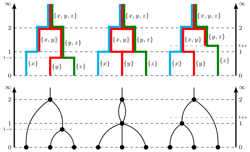
Figure 11: On the top there are three facegrams and on the bottom their associated face-Reeb graphs. On the top of the figure, on the left and to the right of the middle facegram there are two facegrams that are $\varepsilon$-close to it, in the interleaving distance. However, for small $\varepsilon\geq 0$, at least for $\varepsilon$-values that are smaller than half the height of the loop of the middle facegram, the associated Reeb graphs of those facegrams are not $\varepsilon$-close to the middle facegram, since their difference is at least as large as half of the height of the loop of the middle facegram. That means that a small perturbation of the facegrams can lead to a large difference in the face-Reeb graph of the facegrams.

This example motivated us to look for stable invariants of facegrams (our main model of phylogenetic reconstruction). Such an invariant of facegrams should be (i) stable under perturbations of facegrams, (ii) computable, (iii) while capturing as much information as possible. This will be discussed below.

3.2 The mergegram invariant

In this section, we extend the notion of a mergegram from the setting of dendrograms to the setting of facegrams.

Definition 3.3.

Let $C_{X}:(\mathbb{R},\leq)\to\mathbf{Face}(X)$ be a facegram over $X$. We define the mergegram of $C_{X}$ as the multiset of intervals

$$\mathbf{mgm}(C_{X}):=\left\{\left\{I_{\sigma}\mid\sigma\subset X\right\}\right\}\text{, where }I_{\sigma}:=C_{X}^{-1}(\sigma)=\{t\in\mathbb{R}\mid\sigma\in C_{X}(t)\}.$$

Given a $\sigma\subset X$, $I_{\sigma}\subset\mathbb{R}$ is either an interval or $\emptyset$, and it is called the lifespan of $\sigma$ in $C_{X}$.

For an example of a mergegram see Fig. 12. It is easy to check that the mergegram of a facegram corresponds to the edges of the face-Reeb graph of the facegram, viewed as intervals of $\mathbb{R}$. Thus, the face-Reeb graph is more informative than the mergegram. Just as in the case of dendrograms, the mergegram and the Reeb graph of a facegram are topological invariants of the facegram.

Proposition 3.4.

The mergegram of a facegram is invariant of isomorphisms of facegrams.

Proof.

Suppose that $f:X\to Y$ is an equivalence between $C_{X}$ and $C_{Y}$. Since also $f:X\to Y$ is a bijection, for any $\sigma\subset X$, $\sigma$ and $f(\sigma)$ have the same cardinalities. In particular, $\sigma\in C_{X}$ if and only if $f(\sigma)\in C_{Y}$. Thus, $I_{\sigma}=I_{f(\sigma)}$ whenever $I_{\sigma}\neq\emptyset$ and $\sigma\neq\emptyset$. Therefore, $\mathbf{mgm}(C_{X})=\mathbf{mgm}(C_{Y})$. ∎

A refinement of the mergegram

In general, the mergegram is not a complete invariant of facegrams, meaning that there exist different facegrams with the same mergegram. For instance, if we consider a non-tree like facegram and then consider any of its spanning treegrams (viewed as facegrams). These spanning treegrams will contain the same lifespans of edges, and hence the same mergegrams, as the given facegram. We can strengthen the mergegram invariant by considering labeling the lifespans of the edges by their associated simplices. We define this formally as follows.

Definition 3.5.

Let $C_{X}:(\mathbb{R},\leq)\to\mathbf{Face}(X)$ be a facegram over $X$. We define the labelled mergegram of $C_{X}$ as the set

$$\mathbf{mgm}^{*}(C_{X}):=\{(\sigma,I_{\sigma})\mid\emptyset\neq\sigma\subset X\text{ and }I_{\sigma}\neq\emptyset\}.$$

We have the following decomposition result.

Proposition 3.6.

Let $C_{X}:(\mathbb{R},\leq)\to\mathbf{Face}(X)$ be a facegram. For any $t\in\mathbb{R}$ we have

$$C_{X}(t)=\bigvee_{\emptyset\neq\sigma\subset X}C_{X}^{(\sigma)}(t),$$

where the face-set $C_{X}^{(\sigma)}(t)$ is given by

$$C_{X}^{(\sigma)}(t):=\begin{cases}\{\sigma\},&t\in I_{\sigma}\\ \emptyset,&\text{otherwise.}\end{cases}$$

Proof.

The proof follows directly by the fact that every simplicial complex is determined by its clique set of maximal faces. So, we apply this fact point-wisely in the facegram. ∎

Corollary 3.7.

The labelled mergegram $C_{X}\mapsto\mathbf{mgm}^{*}(C_{X})$ is an injection. Hence, it is a complete invariant of facegrams over $X$.

Proof.

Let $C_{X},C^{\prime}_{X}$ be two facegrams over $X$. Suppose that $\mathbf{mgm}^{*}(C_{X})=\mathbf{mgm}^{*}(C^{\prime}_{X})$. Let $I_{\sigma}^{(C_{X})},I_{\sigma}^{(C^{\prime}_{X})}$, $\emptyset\neq\sigma\subset X$, be the lifespans of $C_{X},C^{\prime}_{X}$, respectively. Then, by definition of $\mathbf{mgm}^{*}$, we obtain $(\sigma,I_{\sigma}^{(C_{X})})=(\sigma,I_{\sigma}^{(C^{\prime}_{X})})$, for all $\emptyset\neq\sigma\subset X$. Hence, $C_{X}^{(\sigma)}(t)={C^{\prime}}_{X}^{(\sigma)}(t)$, for all $\emptyset\neq\sigma\subset X$ and all $t\in\mathbb{R}$. By Prop. 3.6, we obtain $C_{X}(t)=C^{\prime}_{X}(t)$, for all $t\in\mathbb{R}$. Therefore, $C_{X}=C^{\prime}_{X}$. ∎

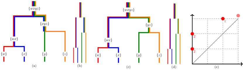
Figure 12: Visualizations (a), (c) of two facegrams having isomorphic face-Reeb graphs (if we forget the labels of their edges) and thus the same mergegrams, however differently labeled. The mergegrams correspond in this visualization to the vertical bars without their labels; (b), and (d) show the bars/intervals $I_{\sigma}$ together with their label; these are the labeled mergegrams of facegrams (a) and (c), respectively. The coloring associated with each interval is the colors of taxa in the clique. Interpreting the mergegram as a persistence diagram gives plot (e), where the multiplicity of the points is given by the numbers next to the points. The opaque point is the point with infinite lifetime. We can see that the mergegrams are the same in (e) or in (b) and (d) when ignoring the coloring of the bars. On the other hand, the labeled mergegram (and the associated coloring of the bars) shows that the two facegrams differ in one face-set, namely $(\{x,y,z\},[2,3))$ and $(\{y,z\},[2,3))$. Finally, note that: the facegram (c) is a dendrogram and in particular a treegram. However, for the facegram (a) its associated face-Reeb graph is a merge tree and yet that facegram is neither a dendrogram nor a treegram. This implies in particular that the facegram (a) is the join span of at least two different treegrams (viewed as facegrams). Moreover, by definition, the face-Reeb graph of a facegram would not be a merge tree if and only if there exists a taxon that can be joined with the root by at least two different consecutive paths of maximal faces through time, and this is clearly not the case for the facegram (a) since $\{x\}$ cannot be joined by a consecutive path of inclusions of maximal faces with $\{x,y,z\}$ through time.

The mergegram of a filtration

In this paragraph, we show how the mergegram of a given facegram can be expressed in terms of the filtration associated with that facegram. This implies that the mergegram can be used as a new topological signature of filtrations without reference to the facegram, suggesting using mergegrams as a new topological signature of filtrations of datasets that can complement the existing toolkit of persistence invariants in TDA.

Proposition 3.8.

Let $C_{X}$ be a facegram over $X$ and let $F_{X}:=\Psi(C_{X})$ be the filtration over $X$ associated to $C_{X}$ via the one-to-one correspondence $(\Phi,\Psi)$ in Thm. 2.31. Let

$$\mathbf{s}(C_{X}):=\left\{\emptyset\neq\sigma\subset X\mid\sigma\in C_{X}(t)\text{, for some }t\in\mathbb{R}\right\}.$$

Given a $\emptyset\neq\sigma\subset X$, $\sigma\in\mathbf{s}(C_{X})$ if and only if $I_{\sigma}$ is a non-empty interval of $\mathbb{R}$. Moreover, for any $\sigma\in\mathbf{s}(C_{X})$, $I_{\sigma}$ is given by the formula

$$I_{\sigma}=\left[F_{X}(\sigma),\min_{\sigma\subsetneqq\tau\subset X}F_{X}(\tau)\right).$$

Moreover, for any $\emptyset\neq\sigma\subset X$, we have:

$$\min_{\sigma\subsetneqq\tau\subset X}F_{X}(\tau)=\min_{\sigma\subsetneqq\tau\in\mathbf{s}(C_{X})}F_{X}(\tau).$$

Hence, the mergegram of $C_{X}$ is given by the following multiset of intervals:

$$\mathbf{mgm}(C_{X})=\left\{\left\{\left[F_{X}(\sigma),\min_{\sigma\subsetneqq\tau\in\mathbf{s}(C_{X})}F_{X}(\tau)\right)\mid\sigma\in s(C_{X})\right\}\right\}.$$

Proof.

The proof is straightforward by definition of $F_{X}$, $I_{\sigma}$ and $s(C_{X})$. ∎

We obtain the following useful corollary.

Corollary 3.9.

Let $C_{X}$ be a facegram over $X$. For any collection $S$ of simplices such that $s(C_{X})\subset S\subset\mathbf{pow}(X)$, we have:

$$\mathbf{mgm}(C_{X})=\left\{\left\{\left[F_{X}(\sigma),\min_{\sigma\subsetneqq\tau\in S}F_{X}(\tau)\right)\mid\sigma\in S\right\}\right\}.$$

Because of Prop. 3.8 which shows the direct expression of the mergegram in terms of the filtration alone, and because of the equivalence between facegrams and filtrations, from now we can also talk about the mergegram of a filtration.

Definition 3.10.

Let $F_{X}:\mathbf{pow}(X)\to\mathbb{R}$ be a filtration over $X$. The mergegram of the filtration $F_{X}$ is defined as

$$\mathbf{mgm}(F_{X}):=\left\{\left\{\left[F_{X}(\sigma),\min_{\sigma\subsetneqq\tau\in\mathbf{pow}(X)}F_{X}(\tau)\right)\mid\sigma\in s(C_{X})\right\}\right\}.$$

Similarly, we can define the labeled mergegram of a filtration, and denote it by $\mathbf{mgm}^{*}(F_{X})$.

3.3 Invariant properties of mergegrams

Although an isomorphism invariant, the mergegram of a filtration is not invariant up to homotopy of filtrations (see Rem. 3.16). However, it turns out that we can consider a particular form of homotopy equivalence of filtrations called weak equivalence, (see Defn. 3.11) under which the mergegram remains invariant (see Prop. 3.15).

Definition 3.11 ([29, Sec. 4.1]).

Let $F_{X}:\mathbf{pow}(X)\to\mathbb{R}$ be a filtration over $X$ and let $\varphi_{X}:Z\twoheadrightarrow X$ be a surjection. Then, we define the pullback filtration $\varphi_{X}^{*}F_{X}$ induced by $F_{X}$ and $\varphi_{X}$, given by

$$\varphi_{X}^{*}F_{X}:\mathbf{pow}(Z) \to\mathbb{R}$$

$$\kappa \mapsto F_{X}(\varphi_{X}(\kappa))$$

Lemma 3.12.

Let $(X,S_{X})$ be a simplicial complex, and let $\varphi_{X}:Z\twoheadrightarrow X$ be a surjection. Let $(Z,\varphi_{X}^{*}S_{X})$ be the pullback complex of $(X,S_{X})$ given by

$$\varphi_{X}^{*}S_{X}:=\{\kappa\subset Z\mid\varphi_{X}(\kappa)\in S_{X}\}.$$

Then, the restriction of the induced map $\varphi_{X}(\cdot):\mathbf{pow}(Z)\to\mathbf{pow}(X)$ from the set of maximal faces of the complexes $(Z,\varphi_{X}^{*}S_{X})$ onto the set of maximal faces of the complex $(X,S_{X})$ is a bijection.

Proof.

Consider the restriction map of $\varphi_{X}(\cdot):\mathbf{pow}(Z)\to\mathbf{pow}(X)$ that maps maximal faces of $\varphi^{*}_{X}S_{X}$ to maximal faces of $S_{X}$. This map is clearly surjective by definition. Now, we claim that this restriction map of $\varphi_{X}(\cdot)$ is also injective. Let $\kappa_{1},\kappa_{2}$ be two maximal faces $\varphi_{X}^{*}S_{X}$ such that $\varphi(\kappa_{1})=\varphi_{X}(\kappa_{2})=:\sigma\in S_{X}$. Consider the union $\kappa_{3}:=\kappa_{1}\cup\kappa_{2}$. Then, $\varphi(\kappa_{3})=\varphi(\kappa_{1}\cup\kappa_{2})=\varphi_{X}(\kappa_{1})\cup\varphi_{X}(\kappa_{2})=\sigma\in S_{X}$. Hence, $\kappa_{3}\in\varphi_{X}^{*}S_{X}$. Because of $\kappa_{1},\kappa_{2}\subset\kappa_{3}$ and because $\kappa_{1},\kappa_{2}$ are maximal faces of the complex $\varphi_{X}^{*}S_{X}$, we conclude that $\kappa_{1}=\kappa_{2}=\kappa_{3}$. Therefore, our surjective map is also injective, and thus a bijection. ∎

Remark 3.13.

Note that although the pullback complex $\varphi^{*}_{X}S_{X}$ is different from the complex $S_{X}$, using Quillen’s theorem A in the simplicial category [32], it was shown by Mémoli that these complexes are homotopy equivalent [29, Cor. 2.1].

The term weak equivalence was used in further generality as an equivalence between objects in certain types of categories [34]. Here, we define this type of equivalence for the case of filtrations.

Definition 3.14.

Let $F_{X},F_{Y}$ be filtrations over the vertex sets $X,Y$, respectively. A pair of surjections $X\xtwoheadleftarrow{\varphi_{X}}Z\xtwoheadrightarrow{\varphi_{Y}}Y$, also called a tripod, is said to be a weak equivalence of $F_{X},F_{Y}$ if their pullbacks along $\varphi_{X}$ and $\varphi_{Y}$ are equal, i.e. $\varphi_{X}^{*}F_{X}=\varphi_{Y}^{*}F_{Y}$. In that case, $F_{X},F_{Y}$ are called weakly equivalent.

Theorem 3.15.

The mergegram is invariant of weak equivalences of filtrations.

Proof.

Let $F_{X}$ and $F_{Y}$ be filtrations over the vertex sets $X$ and $Y$, respectively. Let $C_{X},C_{Y},\varphi_{X}^{*}C_{X}$ be the associated facegrams of $F_{X},F_{Y},\varphi_{X}^{*}C_{X}$, respectively. Suppose that $F_{X}$ and $F_{Y}$ are weakly equivalent. That is, there is a tripod $X\xtwoheadleftarrow{\varphi_{X}}Z\xtwoheadrightarrow{\varphi_{Y}}Y$, such that

$$\varphi_{X}^{*}F_{X}=\varphi_{Y}^{*}F_{Y}.$$ (1)

We claim that $\mathbf{mgm}(F_{X})=\mathbf{mgm}(F_{Y})$. Because of Eqn. (1), it suffices to show the equality $\mathbf{mgm}(F_{X})=\mathbf{mgm}(\varphi^{*}F_{X})$. By surjectivity of $\varphi_{X}$, it follows that those mergegrams can only be different on the multiplicities of some of their intervals. Now, we need to craft a bijection between those multisets, that preserves their multiplicities. We consider the map

$$\overline{\varphi}_{X}:\mathbf{mgm}(\varphi_{X}^{*}F_{X}) \mapsto\mathbf{mgm}(F_{X})$$

$$I_{\kappa} \mapsto I_{\varphi_{X}(\kappa)}$$

This map is surjective counting multiplicities, since $\varphi_{X}$ is surjective. By Lem. 3.12, the map of maximal faces, $k\mapsto\varphi_{X}(k)$, is bijective. Hence, the map $I_{\kappa}\mapsto I_{\varphi_{X}(\kappa)}$ is a bijection which preserves multiplicities. Thus, the mergegrams are equal.

∎

Remark 3.16.

It follows by Lem. 3.12 that the number of maximal faces of a simplicial complex is invariant of pullbacks. However, the number of maximal faces of a complex is not invariant up to homotopy equivalence of complexes: to see this, consider two complexes $S_{X}$ and $S_{Y}$, where $S_{X}$ is a triangle and $S_{Y}$ is the complex obtained by gluing two triangles along a common edge. These complexes are clearly homotopy equivalent, however, they have a different number of maximal faces ($1$ and $2$ respectively). This implies that the mergegram, although invariant of weak equivalences, is not invariant up to homotopy equivalence of filtrations.

Corollary 3.17.

Let $(X,N_{X}),(Y,N_{Y})$ be two phylogenetic networks (e.g. finite metric spaces). Let $\mathbf{VR}_{X}:\mathbf{pow}(X)\to\mathbb{R}$ and $\mathbf{VR}_{Y}:\mathbf{pow}(Y)\to\mathbb{R}$ be the associated Vietoris-Rips filtrations. If there exists an isometry $\varphi:X\to Y$ between those networks, then $\mathbf{mgm}(\mathbf{VR}_{X})=\mathbf{mgm}(\mathbf{VR}_{Y})$.

3.4 Stability of the mergegram

We define the bottleneck distance for comparing mergegrams and an $\ell^{\infty}$-type of metric for comparing labeled mergegrams. Then, we show that the mergegram invariant of filtrations is $1$-Lipschitz stable in the perturbations of the tripod distance on filtrations.

Since mergegrams are multisets of intervals, they can be thought of as persistence diagrams. Thus, we can consider the bottleneck distance as a metric for the comparison of mergegrams.

Definition 3.18 (Bottleneck distance).

Let $A,B$ be a pair of multisets of intervals. Let $\varepsilon\geq 0$. An $\varepsilon$-matching of $A,B$ is a bijection $\varphi:A^{\prime}\to B^{\prime}$ between a subset $A^{\prime}\subset A$ and $B^{\prime}\subset B$ such that

1. for every $I=[a,b]\in A^{\prime}$ and $\varphi(I)=[c,d]\in B^{\prime}$, $||(a,b)-(c,d)||_{\infty}\leq\varepsilon\text{, and }$

2. for every $[a,b]\in(A\setminus A^{\prime})\cup(B\setminus B^{\prime})$, $|a-b|\leq 2\varepsilon$.

The bottleneck distance of $A,B$ is defined as

$$d_{\mathrm{B}}(A,B):=\inf\{\varepsilon\geq 0\mid\text{there exists an }\varepsilon\text{-matching of }A,B\}.$$

We consider an $\ell^{\infty}$-type of metric for comparing labeled mergegrams over $X$.

Definition 3.19.

Let $C_{X},C^{\prime}_{X}$ be facegrams over $X$, respectively. Their $\ell^{\infty}$-distance is

$$d_{\infty}(\mathbf{mgm}^{*}(C_{X}),\mathbf{mgm}^{*}(C^{\prime}_{X})):=\max_{\sigma\in\mathbf{pow}(X)}d_{\mathrm{B}}(I_{\sigma}^{C_{X}},I_{\sigma}^{C^{\prime}_{X}}).$$

We can also consider a tripod-like distance for comparing labeled mergegrams over different sets, however, we are not intending to use such a distance in this paper, so we omit such a definition.

Proposition 3.20.

Let $X$ be a taxa set. Let $F_{X},F^{\prime}_{X}$ be two filtered simplicial complexes over $X$ and let $C_{X}$ and $C^{\prime}_{X}$ be their associated facegrams. Then, we have the following bounds

$$d_{\mathrm{B}}(\mathbf{mgm}(F_{X}),\mathbf{mgm}(F^{\prime}_{X}))\leq d_{\infty}(\mathbf{mgm}^{*}(C_{X}),\mathbf{mgm}^{*}(C^{\prime}_{X}))\leq d_{\mathrm{I}}(C_{X},C^{\prime}_{X})=d_{\mathrm{I}}(F_{X},F^{\prime}_{X}).$$

Proof.

The equality follows directly from the fact that the lattice of face-sets is isomorphic to that of simplicial complexes and applying the property of the interleaving distance that the associated persistent structures are interleaving isometric (see Bubenik et al. [4, Sec. 2.3]). Assume that $d_{I}(C_{X},C^{\prime}_{X})\leq\varepsilon$. That means that $C_{X}(t)\leq C^{\prime}_{X}(t+\varepsilon)$ and $C^{\prime}_{X}(t)\leq C_{X}(t+\varepsilon)$. This in turn implies that each of the lifespans of the intervals in the labeled mergegram is of length at most $\varepsilon$. This explains the bound with the labeled mergegram. Since the $d_{\infty}$ distance of labeled mergegrams is an $\ell^{\infty}$-type of metric, this bound also implies that there is a canonical $\varepsilon$-matching $I_{\sigma}^{(C_{X})}\mapsto I_{\sigma}^{(C^{\prime}_{X})}$ between the intervals of the ordinary mergegrams $\mathbf{mgm}(C_{X})$ and $\mathbf{mgm}(C^{\prime}_{X})$. So, the bottleneck distance of the ordinary mergegrams is at most $\varepsilon$ too. ∎

Next, we establish the stability of the mergegram by following the same strategy as in [29] and other works of Mémoli et al., e.g. [23]. More precisely, now that we have established the invariance of mergegrams under weak equivalences of filtrations (Thm. 3.15), we show the stability of the mergegram invariant by invoking stability for the invariant when the underlying sets are the same.

Proposition 3.21 ($1$-Lipschitz stability of the mergegram).

Let $X$ and $Y$ be two finite sets.

• Let $F_{X},F_{Y}$ be a pair of filtrations over $X$ and $Y$, respectively. Then

  $$d_{\mathrm{B}}(\mathbf{mgm}(F_{X}),\mathbf{mgm}(F_{Y}))\leq d_{\mathrm{T}}(F_{X},F_{Y}).$$

• Let $(X,N_{X}),(Y,N_{Y})$ be a pair of phylogenetic networks (e.g. finite metric spaces) and let $\mathbf{VR}_{X},\mathbf{VR}_{Y}$ be their Vietoris-Rips filtrations. Then

  $$d_{\mathrm{B}}(\mathbf{mgm}(\mathbf{VR}_{X}),\mathbf{mgm}(\mathbf{VR}_{Y}))\leq d_{\mathrm{GH}}((X,N_{X}),(Y,N_{Y})).$$

Proof.

Let $X\xtwoheadleftarrow{\varphi_{X}}Z\xtwoheadrightarrow{\varphi_{Y}}Y$ be a tripod between $X$ and $Y$. We have

$$d_{\mathrm{B}}(\mathbf{mgm}(F_{X}),\mathbf{mgm}(F_{Y})) =d_{\mathrm{B}}(\mathbf{mgm}(\varphi_{X}^{*}F_{X}),\mathbf{mgm}(\varphi_{Y}^{*}F_{Y}))$$

$$\leq d_{\mathrm{I}}(\varphi_{X}^{*}F_{X},\varphi_{Y}^{*}F_{Y}).$$

Since the tripod was arbitrary, by taking infimums over all tripods, we obtain

$$d_{\mathrm{B}}(\mathbf{mgm}(F_{X}),\mathbf{mgm}(F_{Y}))\leq d_{\mathrm{T}}(F_{X},F_{Y}).$$

The second claim follows directly by Rem. 2.44. ∎

Example 3.22.

Consider the three facegrams from Fig. 11. We can see in the figure below that the mergegrams of those facegrams are at most $\varepsilon$-close to each other in the bottleneck distance.

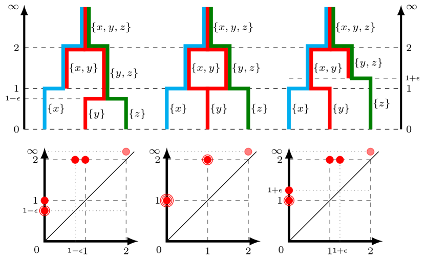
Figure 13: Facegrams and their respective mergegrams. Points with multiplicity $2$ and $3$ are shown by drawing multiple rings around a point.

4 Computational aspects

In this section, we investigate (i) the complexity of computing the join-span of a family of treegrams in the lattice of cliquegrams and in the lattice of facegrams, respectively, and the (ii) complexity of computing the mergegram for these cases. As we describe in the Table 1, we have two different classes of inputs (the top one which is motivated by phylogenetic reconstruction and the bottom one which is motivated by TDA) for which we want to compute the mergegrams of the respective cliquegram or facegram structures. In the following, we will either describe how to pass along each arrow and what to be careful of or give pseudo-code for the computations. As can be seen, there are 4 different paths to be taken from the inputs to their mergegrams.

Table 1: Overview over the algorithmic structures. To compute the join of treegrams we can use the join operation of the lattice of cliquegrams or of facegrams and then calculate the respective mergegram invariants. Similarly, we can compute the mergegram for metric spaces either using cliquegrams or facegrams. The arrows represent the different paths to be taken and represent different algorithms to be used.

In the case of cliquegram we exploit the representation via a phylogenetic network for computational efficiency, i.e. a $n\times n$-matrix for $n$ being the number of common taxa, since there exists a one-to-one correspondence due to Prop. 2.17. Furthermore, the different values in the matrix correspond to the different values in the critical set of the associated cliquegram. For facegrams such a representation via matrices does not exist, and we use the face-sets with their respective filtration values.

4.1 The mergegram of a cliquegram

Join-cliquegram

Given a set $\{U^{1}_{X},\ldots,U_{X}^{\ell}\}$ of $\ell$ symmetric ultranetworks over a set of taxa $X=\{x_{1},\ldots,x_{n}\}$, the join-cliquegram $C_{X}:=\vee_{i=1}^{\ell}T_{X}^{i}$ of their associated treegrams $T_{X}^{i}:=\varphi(U_{X}^{i})$, $i=1,\ldots,\ell$ can be computed as mentioned in Remark 2.20:

1. Take the minimizer matrix (entry-wise minimum of the symmetric ultranetworks over all associated treegrams). The minimizer matrix is a symmetric network, more specifically a phylogenetic network.

2. Compute the associated cliquegram for the minimizer matrix - this is the join-cliquegram - using Algorithm 1. The different values in the minimizer matrix will be the different values of the critical set of the cliquegram.

3. Compute the mergegram of that cliquegram, via Algorithm 2.

Algorithm 2 The mergegram of a cliquegram

1:Given a cliquegram $\mathcal{C}_{X}:\mathbb{R}\to\mathbf{Cliq}(X)$, with critical set $\epsilon_{1}<\epsilon_{2}<\ldots<\epsilon_{s}$.

2:Initialize $M~{}\leftarrow~{}\{(\sigma,\epsilon_{1},\infty)|\sigma\in C_{X}(\epsilon_{1})\}$

3:for all $i\in\{1,\ldots,s-1\}$ do

4:     for all $\sigma\in\mathcal{C}_{X}(\epsilon_{i+1})~{}\backslash~{}\mathcal{C}_{X}(\epsilon_{i})$ do $\triangleright$ All these cliques appear when $\epsilon_{i}\curvearrowright\epsilon_{i+1}$.

5:         $M~{}\leftarrow~{}M\cup\{(\sigma,\epsilon_{i+1},\infty)\}$ $\triangleright$ Add newly born clique (it appeared in $\epsilon_{i+1}$)

6:     end for

7:

8:     for all $\sigma\in\mathcal{C}_{X}(\epsilon_{i})~{}\backslash~{}\mathcal{C}_{X}(\epsilon_{i+1})$ do $\triangleright$ All these cliques disappear when $\epsilon_{i}\curvearrowright\epsilon_{i+1}$.

9:         Let $(\sigma,\epsilon,\infty)$ be the existing entry in $M$ starting with $\sigma$.

10:         $M~{}\leftarrow~{}M\setminus\{(\sigma,\epsilon,\infty)\}$ $\triangleright$ Remove entry

11:         $M~{}\leftarrow~{}M\cup\{(\sigma,\epsilon,\epsilon_{i+1})\}$ $\triangleright$ Add the entry updated with its death time.

12:     end for

13:end for

14:Return $M$ $\triangleright$ Return the labelled mergegram

Let $M_{1},M_{2},\ldots,M_{s}$ the clique-sets corresponding to each value in the critical set $\epsilon_{1}<\ldots<\epsilon_{s}$ of $C_{X}$. By the definition of critical set, the clique-sets are trivial, i.e. $C_{X}(t)=\emptyset$, for $t<\epsilon_{1}$ and $C_{X}(t)=X$ for $t\leq\epsilon_{s}$. Given the ultranetwork representations of treegrams as input, the asymptotic complexity of calculating the minimizer matrix is $O(s\cdot n^{2})$, since it depends linearly on the number $s$ of all different critical points of all the trees (this corresponds to the number of all different values of the entries of all the ultranetworks) and quadratic on the number of taxa, $n$ (since the minimizer matrix is the $n\times n$-matrix obtained by taking entry-wise minima over all the entries of all the ultranetworks of the treegrams).

The calculation of the maximal cliques for each step in the intermediate graph $G_{t}$ in step $2$ is the costly step in this pipeline: In terms of the number of taxa, $n:=|X|$ alone as input parameter the computation is certainly costly: variants of the Bron-Kerbosch algorithms [3] are still the best general case running cases for finding all maximal cliques in such a graph, resulting in a worst-case runtime of $\mathcal{O}(s3^{n/3})$ for $s$ being the size of the critical set of the cliquegram and $n$ the number of vertices in the graph. In our case $n$ is the number of taxa, i.e. $n=|X|$.

In terms of the set of all cliques as a complexity parameter, the computation of the mergegram of the cliquegram is done in $\mathcal{O}(s|M|)$ where $|M|$ is the number of maximal cliques over all values of the critical set which is bounded above by $2^{|X|}$, i.e. $M:=\bigcup M_{i}$. Specifically, we have these bounds for the two inner loops and computing the set-differences

$$O\left((s-1)2|M|+\sum_{i=1}^{s-1}2\min(|M_{i}|,|M_{i+1}|)\right)=O(s|M|+(s-1)|M|)=O(s|M|).$$

Remark 4.1.

Using optimized data-structures for the representation of the cliquegram the theoretical complexity for computing the cliquegram associated to a distance matrix is the same as for computing the Rips complex for the Critical Simplex Diagram in [2] where it is stated to be $\mathcal{O}(|M|^{2.38})$ for $|M|$ being the sum of all maximal faces.

Cliquegram of a metric space

Given a metric space with $n$ points, we can consider the $n\times n$-distance matrix of the distance of each of the points from each other. Since any such distance matrix is also a phylogenetic network (with the diagonals being zero), we can compute the associated cliquegram and its mergegram as we did above, without having to compute the minimizer matrix.

4.2 The mergegram of a facegram and its complexity

Join-facegram: complexity

We show that the complexity of computing the join-facegram of a set of treegrams and then its associated mergegram invariant is polynomial in the input parameters.

First, we need the following technical results.

Proposition 4.2.

Let $C_{X}^{k}$, $k=1,\ldots,\ell$ be a finite collection of face-set over $X$. Let $C_{X}:=\bigvee_{k\in\{1,\ldots,\ell\}}C_{X}^{k}$. Then,

$$C_{X}=\left\{\sigma\subset\bigcup_{k\in\{1,\ldots,\ell\}}C_{X}^{k}\mid\sigma\nsubseteq\tau,\text{ for all }\tau\in\left(\bigcup_{k\in\{1,\ldots,\ell\}}C_{X}^{k}\right)\setminus\{\sigma\}\right\}.$$

In other words, the join of the $C_{X}^{k}$’s consist of the set of maximal elements in the union $\bigcup_{k\in\{1,\ldots,\ell\}}C_{X}^{k}$. In particular, $C_{X}\subset\bigcup_{k\in\{1,\ldots,\ell\}}C_{X}^{k}$.

Proof.

Because of the lattice isomorphism between simplicial complexes and face-set in Prop. A.2, the proof follows by recasting the problem in the setting of simplicial complexes; see Rem. 2.27. Hence, the maximal faces of a union of complexes are computed by the above formula. ∎

Corollary 4.3.

Given a set of $\ell\geq 2$ face-sets over $X$ $\{C^{1}_{X},\ldots,C^{\ell}_{X}\}$, the join-face-set $C_{X}:=\bigvee_{i\in\{1,\ldots,\ell\}}C^{i}_{X}$ can be computed in time at most $O\left(\left(\sum_{i=1}^{\ell}|C^{i}_{X}|\right)^{2}\max|C^{i}_{X}|\right)$ .

Proof.

Consider $C\in\bigcup_{k\in\{1,\ldots,\ell\}}C_{X}^{k}$. In the construction of $\bigvee_{k\in\{1,\ldots,\ell\}}$ we need to check if $C$ is not contained in another element in $\bigcup_{k\in\{1,\ldots,\ell\}}C_{X}^{k}$. To check this, we need to perform $\sum_{i=1}^{\ell}|C^{i}_{X}|$ comparison of $C$ to other elements of the union. The cost of each comparison is bounded by $max|C^{i}_{X}|$. Since there are $\sum_{i=1}^{\ell}|C^{i}_{X}|$ elements $C$ for which the check need to be done, the computational complexity of the procedure is $O\left(\left(\sum_{i=1}^{\ell}|C^{i}_{X}|\right)^{2}\max|C^{i}_{X}|\right)$. ∎

Theorem 4.4.

Given a set $\{U^{1}_{X},\ldots,U_{X}^{\ell}\}$ of $\ell$ symmetric ultranetworks over a set of taxa $X=\{x_{1},\ldots,x_{n}\}$, (i) the join-facegram $C_{X}:=\vee_{i=1}^{\ell}T_{X}^{i}$ of their associated treegrams $T_{X}^{i}:=\varphi(U_{X}^{i})$, $i=1,\ldots,\ell$, (ii) the labelled mergegram $\mathbf{mgm}^{*}(C_{X})$, (iii) the Reeb graph and (iv) the unlabeled mergegram $\mathbf{mgm}(C_{X})$ of $C_{X}$, can all be computed in time at most $O(n^{4}\cdot\ell^{2})$.

Proof.

Since the mergegram can directly be obtained by the labelled mergegram (by projecting its elements to the second coordinate), and since the labelled mergegram is complete invariant for facegrams, among (i), (ii) and (iv), it suffices to show our complexity claim only for computing the labelled mergegram. Also for (iii) as well: computing the Reeb graph of a facegram is not more complicated than the descriptive complexity of facegram and of the labelled mergegram, having an upper bound on the computational complexity of the labelled mergegram, will yield an upper bound on the complexity of computing the Reeb graph.

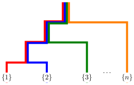
Figure 14: Example of a tree with the maximal number of different height values which are $2n-1$ for $n$ taxa/leaves.

First, observe that for each treegram $T_{X}^{i}$, viewed as a facegram, the number of different simplices in it, will be no more than the number of its edges, which is one number less than the number of its vertices. Because of the tree structure in $T_{X}^{i}$, the number of its vertices is upper bounded by: the product of

• the number of different distance values in the matrix $U_{X}^{i}$, which is no larger than $2n-1$: because of the tree structure of $T^{i}_{X}$, there are at most $2n-1$ different height values for the tree; the value $n$ can be attained when the treegram is as in Fig. 14 (for this type of treegrams, there are $n$ leaf nodes and there are $(n-1)$ tree nodes, so $(2n-1)$ in total), and

• the number of all possible vertices of a fixed height, which is no larger than $n$: because vertices of fixed height are at most as many as the cardinality of the level set of a fixed height which is a partition of the taxa set $X$ and the cardinality of it is at most $n$ because the finest partition is $\{\{x\}\mid x\in X\}$ which has cardinality same as $|X|=n$.

Hence, the number of all different simplices in each treegram is at most $n\cdot(2n-1)$. Now, consider the set $S$ of all different simplices appearing in the treegrams $\{T_{X}^{i}\}_{i=1}^{\ell}$ (viewed as facegrams). By the subsequent argument $|S|\leq n\cdot(2n-1)\cdot\ell$.

The join–filtration $F_{X}$ of the tree filtrations associated to the ultrametrics $U^{k}_{X}$, $k=1,\ldots,\ell$, is given point-wise for every $\sigma\in\mathbf{pow}(X)$ by the formula:

$$F_{X}(\sigma)=\min_{k\in\{1,\ldots,\ell\}}\left(\max_{x_{i},x_{j}\in\sigma}U^{k}_{X}(x_{i},x_{j})\right).$$

By the second conclusion of Prop. 4.2, the definition of $S$ and that $C_{X}=\bigvee_{i=1}^{\ell}T^{i}_{X}$, we obtain that $S\supset s(C_{X})$. By Prop. 3.8 and Cor. 3.9, the mergegram can be computed by using the set $S$ of simplices. Hence, there are at most $|S|$ non-empty intervals to compute to decide if they are non-empty, which is $O(n^{2}\cdot\ell)$. Now, once we have a simplex $\sigma\in S$, to decide if

$$\min_{\sigma\nsubseteq\tau\in S}F_{X}(\tau)>F_{X}(\sigma)$$

takes $|S|$-steps (taking all possible $\tau\in S$) which is again $O(n^{2}\cdot\ell)$. Therefore, computing the labelled mergegram $\mathbf{mgm}^{*}(C_{X})$ and thus the join-facegram $C_{X}$ from the given set of ultranetworks, take time at most $O(n^{4}\cdot\ell^{2})$. ∎

Remark 4.5.

The intuition behind Thm. 4.4, is that by Rem. 2.27 the information of all maximal simplices in the join of the facegrams is already given by the collection of maximal simplices of the facegrams of the trees. This is not the case for cliquegrams where we need to find maximal cliques for the different filtration levels, either in the case of constructing the join cliquegram from (cliquegrams of) the treegrams or when squashing the loops in the facegram. Thus, the cliquegram construction and therefore the calculation of the mergegram of cliquegram might need exponential time.

Join-facegram: algorithms

In the following, we list two algorithms for the mergegram of the join facegram. Algorithm 3 is still close to the actual implementation; we could just say: make a huge union of all $(\sigma,I_{\Sigma})$ and then just take the smallest filtration value of $\sigma$ over all such pairs. A bit more precisely, the algorithm to calculate the labelled mergegram first collects all different pairs $(\sigma,I_{\sigma})$ for a fixed $\sigma$ in all the labelled mergegrams of the treegrams to get the minimal birth time $\min_{i}F_{T^{i}}(\sigma)$ and minimal death time $\min_{i}F_{T^{i}}(\tau_{i})$ for $\tau_{i}\supset\sigma$. Then the labelled mergegram for the join of the treegrams is directly given by this collection.

Algorithm 3 The mergegram of the join facegram of the facegram of treegram (Version 1)

1:Let $\mathbf{mgm}^{*}(T^{i}_{X})$ be the labelled mergegrams of the treegrams for $i\in\{1,\ldots,l\}$.

2:Let $S=\emptyset$, $L=\emptyset$

3:for all $i\in\{1,\ldots,l\}$ do

4:     for all $(\sigma,I_{\sigma})\in\mathbf{mgm}^{*}(T^{i}_{X})$ do

5:         if $\sigma\not\in S$ then

6:              $S=S\cup\{\sigma\}$

7:              $L=L\cup\{(\sigma,I_{\sigma})\}$

8:         else

9:              let $(\sigma,I)\in L$ be the labelled interval in $L$; $I_{\sigma}=[a_{0},b_{0})$, $I=[a_{1},b_{1})$.

10:              $L=L\backslash\{(\sigma,I)\}$.

11:              $L=L\cup\{(\sigma,[\min(a_{0},a_{1}),\min(b_{0},b_{1}))\}$.

12:         end if

13:     end for

14:end for

15:Return $L$

The algorithm relies on the fact that for the associated ultranetworks for the tree distances for each $(\sigma,I_{\sigma})$ in a treegram, the distance between taxa in the face-set $\sigma$ are smaller than the distances between points in $\sigma$ and outside of it, that is

$$\max_{y\in\sigma}\max_{x\in\sigma}U^{i}_{X}(x,y)\leq\min_{y\not\in\sigma}\max_{x\in\sigma}U^{i}_{X}(x,y),$$

since this would otherwise violate the condition of the lattice structure of $\mathbf{Facegm}(X)$. Therefore, to get the mergegram of the join facegram, we have to consider all the labelled intervals in all the treegrams.

Algorithm 4 The mergegram of the join facegram of a set of treegrams (Version 2)

1:Let $\mathbf{mgm}^{*}(T^{i}_{X})$ be the labelled mergegrams of the treegrams for $i\in T:=\{1,\ldots,l\}$ and $U^{i}_{X}$ its corresponding ultranetwork.

2:Let $S=\emptyset$ $\triangleright$ Set holding the simplices visited.

3:and $L=\emptyset$ $\triangleright$ Labelled intervals of the joined facegram.

4:for all $\sigma\in\{\tau~{}|~{}\exists i\in T~{}\exists I\text{ interval s.t. }(\tau,I)\in\mathbf{mgm}^{*}(T^{i}_{X})\}$ do

5:     if $\sigma\not\in S$ then

6:         $S=S\cup\{\sigma\}$

7:         $a=\min_{i\in T}\max_{y\in\sigma}\max_{x\in\sigma}U^{i}_{X}(x,y)$

8:         $b=\min_{i\in T}\min_{y\not\in\sigma}\max_{x\in\sigma}U^{i}_{X}(x,y)$

9:          

10:         if $a<b$ then$\triangleright$ By definition of the treegrams, we always have $a\leq b$.

11:              $L=L\cup\{(\sigma,~{}[a,b)~{})\}$

12:         end if

13:     end if

14:end for

15:Return $L$

Remark 4.6.

In general, the possibly computationally expensive part of the computation of the mergegram of a facegram is the construction of the facegram itself. In the case of the facegram arising as the join of treegrams, all the necessary information is already encoded in the collection of all the labelled mergegrams of the treegrams, and we can compute it in polynomial time. Furthermore, for a given facegram representation, we can calculate the mergegram of it in at most $\mathcal{O}(M^{2})$ time, where $M$ is the number of different faces.

Remark 4.7.

It should be noted that for the mergegram each simplex can only contribute to at most one non-trivial interval to the mergegram. Alg. 3 takes this into account by explicitly matching the simplices with an appropriate interval. In Alg. 4 this matching is done implicitly using just the appropriate minimal/maximal values in the ultramatrices of the treegrams. This leads to major speed-ups in the algorithm.

Metric space reconstruction via facegram

Instead of representing a metric space as a cliquegram, we can also use the facegram representation. Opposed to the cliquegram - which gives the same result as the Rips-complex in terms of maximal cliques and their filtration values - we have the flexibility of choosing any filtration on the metric space to build our facegram.

1. Given a finite metric space $M$ (e.g. a point cloud) with $n$ points, label these with $1,2,\ldots,n$.

2. Choose a filtration on the metric space, e.g. the Alpha complex [15].

3. Sort the different filtration values and obtain the maximal faces for each of the filtration values, to obtain the facegram of the metric space.

4. Compute the mergegram of that facegram.

For an implementation of these steps, see [14] for a more detailed explanation. In general, the hurdles for the implementation are to find a quick implementation for the desired filtration which lends itself to fast construction of the facegram. Obtaining the mergegram from the facegram can then be done in the same fashion as for the cliquegram using Algorithm 2.

4.3 Experiments with datasets

We examine the mergegram of the join-facegram, first to an artificial dataset and then to a benchmark biological dataset.

Artificial dataset

Let us consider two randomly chosen dendrograms given in Fig. 15. There exist several ways to construct random dendrograms, one is to choose a random distance matrix and use UPGMA (unweighted pair group method with arithmetic mean) hierarchical clustering method. For random treegrams other hierarchical clustering algorithms like single-linkage clustering can be used. The respective mergegrams of the dendrograms constructed are shown in 16.

Figure 15: The dendrograms of two random trees. The coloring is corresponding to certain clusters by scipy.

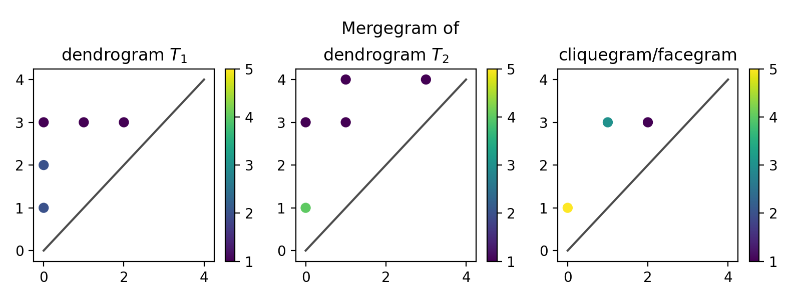
Figure 16: The mergegrams of the two random trees (left and middle). Treegrams viewed as either cliquegrams or facegrams always give the same mergegram. Coloring is done by the multiplicity of each point. Mergegram of the join-cliquegram and of the join-facegram (right) of the two treegrams are the same in this case. Coloring is done by the multiplicity of each point.

For these two dendrograms we can now compute their join-cliquegram as well as their join-facegram, in the respective lattices of cliquegrams and facegrams. In this case, both the join of cliquegrams and the join of facegrams coincide: we get three different points in the mergegram all with different multiplicities. On the other hand, the join-cliquegram and join-facegram may differ, depending on the subpartitions. An example are the dendrograms in Fig. 17. The mergegrams of the treegrams and the distinct mergegrams of the join-cliquegram and join-facegram are shown in 18 and 19 respectively.

Figure 17: Three different dendrograms on the same taxa set.

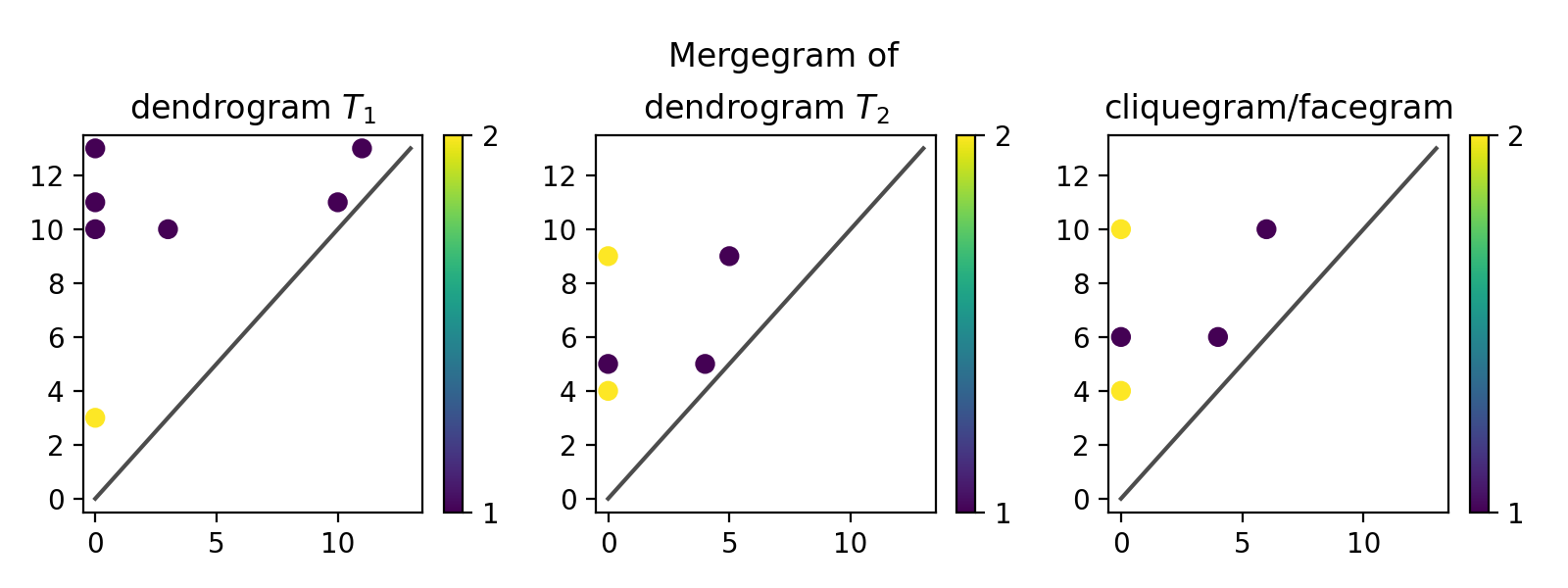
Figure 18: The mergegrams of the treegrams shown in 17.

While the birth-/death-times are the same for the singletons for both cliquegram and facegram in Fig. 19, there is one more point in the mergegram of the join-cliquegram while the lifespans of these points are less (or equal) to the ones in the join-facegram.

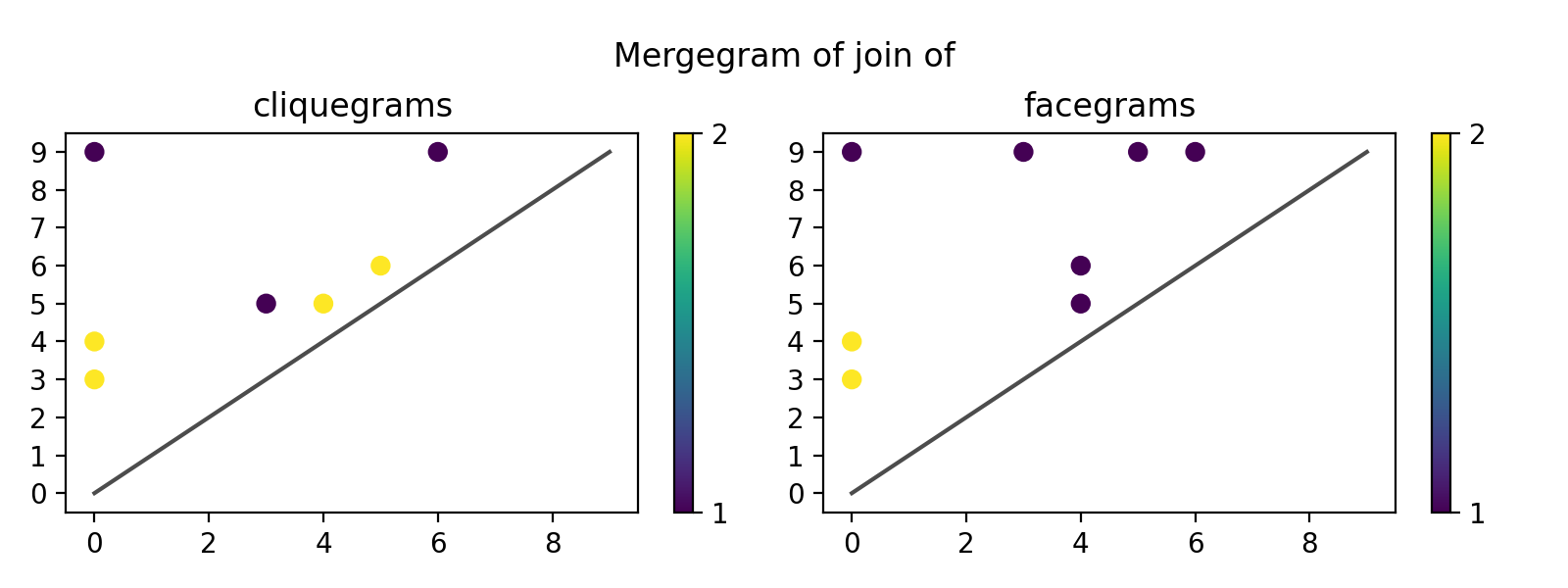
Figure 19: The mergegrams of the joins of the treegrams in 17.

Biological data set

In the following, we use some trees coming from real phylogenetic trees in [35] to compute their join in the cliquegram and facegram settings. We have selected $68$ common taxa for $161$ dendrograms, two of which are shown in Fig. 20.

mean	standard deviation	minimum	maximum
0.3499	0.1110	0.1117	0.9120

Table 2: Summary statistics of all the bottleneck distances of the mergegrams of different treegrams.

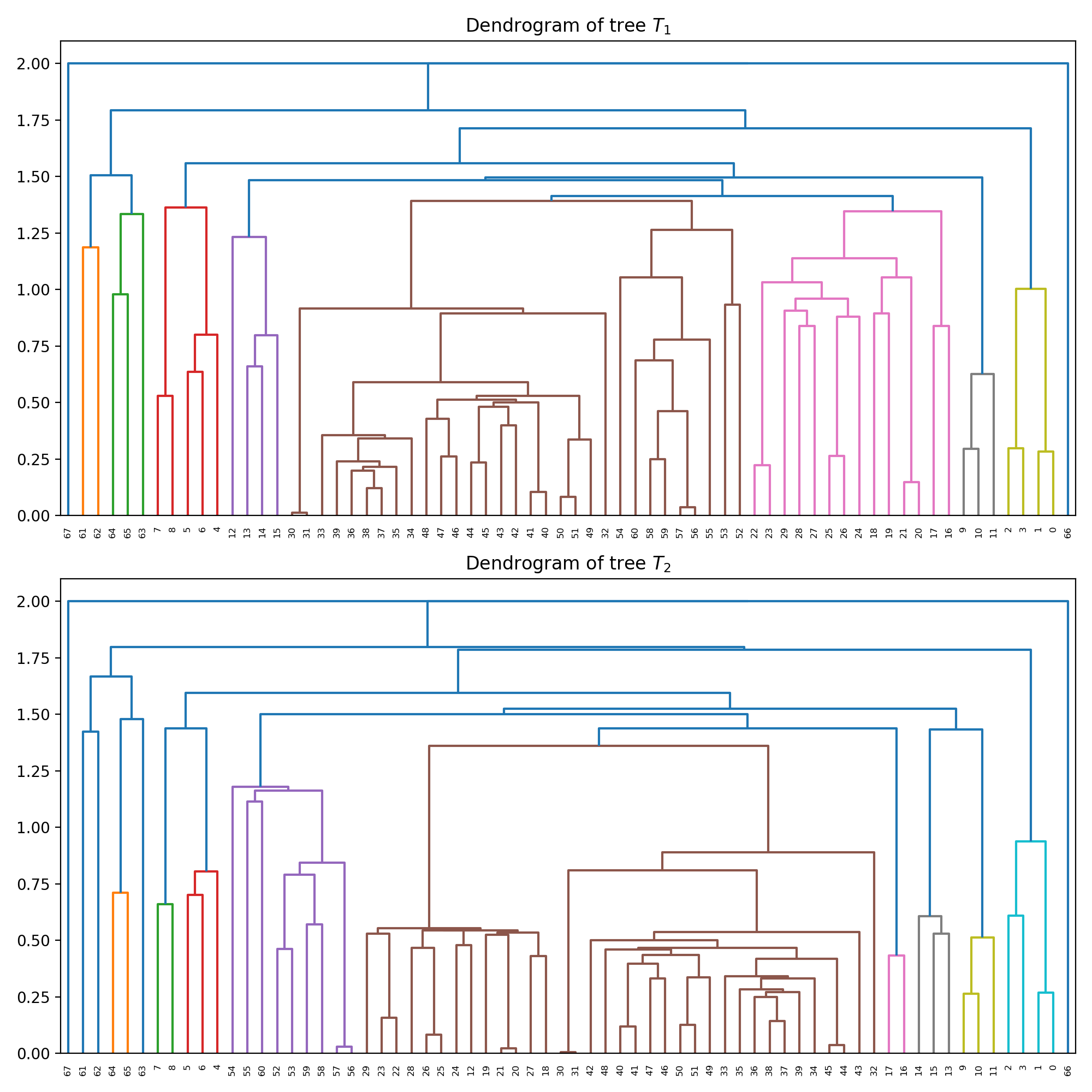
Figure 20: The dendrograms of two trees from the 161 different trees available for this dataset.

Figure 21: The mergegrams of the join cliquegram and the join facegram, respectively, for all 161 trees. The two mergegrams are nearly identical with a bottleneck distance of $1e^{-15}$.

Bottleneck distance of mergegrams

As mentioned before, we can interpret the mergegram as a persistence diagram and can therefore use distances like the bottleneck distance to compare two mergegrams with each other. To highlight one further property of the join of cliquegrams and facegrams, we consider the following setting:

Given a network with $21$ spanning trees over a common taxa set $X=\{x_{1},\ldots,x_{n}\}$ of $n$ taxa and their treegrams $T_{X}^{1},\ldots,T_{X}^{21}$, compute the join cliquegrams $C_{X}^{k}=\bigvee_{i=1}^{k}T_{X}^{i},$ where $k=1,\ldots,21$. Now compute the bottleneck distances $d_{\mathrm{B}}$ between the mergegrams of these join spans with the mergegram of the join of all treegrams, i.e.

$$d_{\mathrm{B}}(\mathbf{mgm}(C_{X}^{k}),\mathbf{mgm}(C_{X}^{21})).$$

Analogously, we can do the same construction for the join-facegram. Fig. 22 shows the plots of these distances for different numbers of leaves of the network having $21$ spanning trees each. The bottleneck distances decrease until we reach a distance of zero at the end. This highlights the property of the join again of being the smallest cliquegram/facegram encoding the information given in the trees.

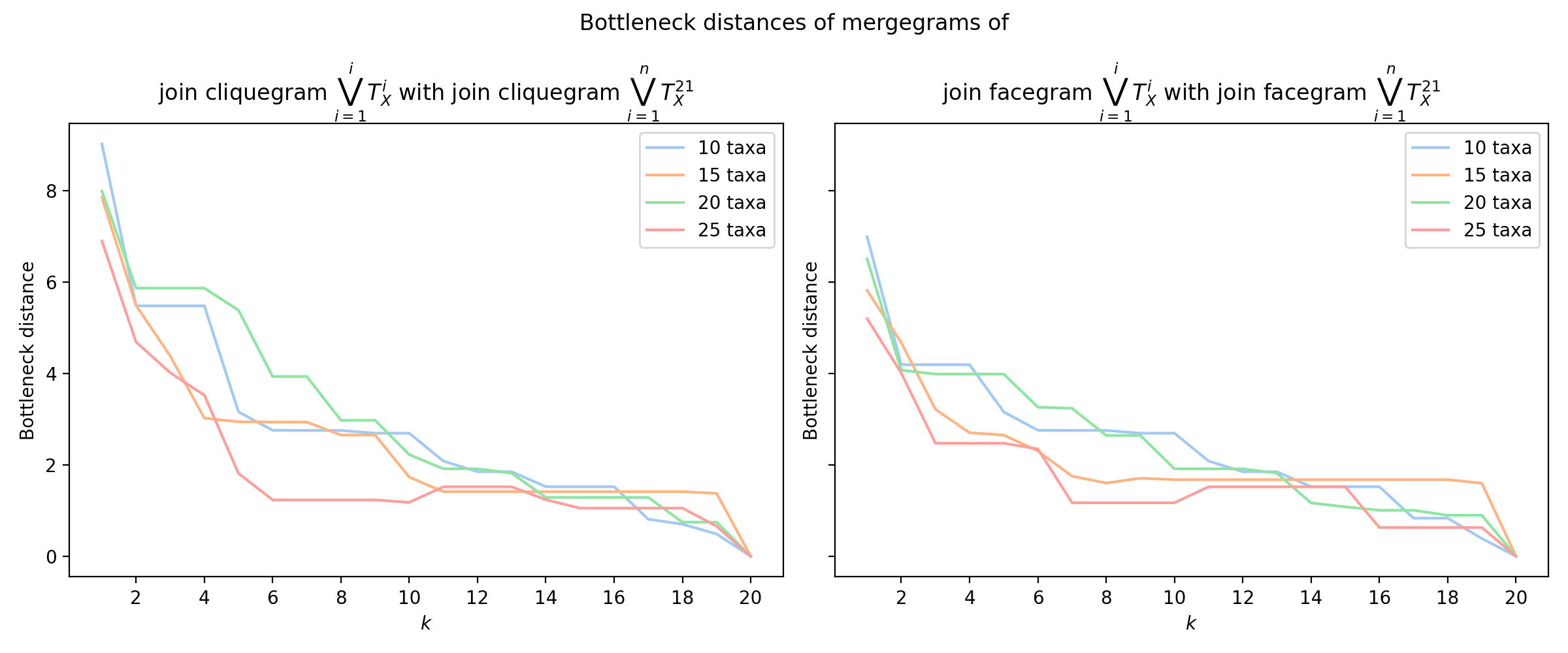
Figure 22: Progression of bottleneck distances between the mergegram of the join of the first $n$ treegrams and the mergegram of the join of all 21 treegrams for different number of taxa for the case of cliquegrams and facegrams.

Appendix A Postponed proofs

Below, we provide detailed combinatorial topological proofs of some of the concepts we used. For a detailed introduction in combinatorial algebraic topology, we refer to the book of Kozlov [25].

Proposition A.1.

Let $X$ be a set of taxa. There is a natural isomorphism

$$\mathbf{Cliq}(X)\stackrel{{\scriptstyle[}}{{\mathbf{}}}{Cliq}]{\mathbf{Grph}}{\rightleftarrows}\mathbf{Grph}(X)$$

between the lattice $\mathbf{Cliq}(X)$ of all clique-sets over $X$ and the lattice $\mathbf{Grph}(X)$ of all graphs over $X$, where the maps are defined as follows

• For any clique-set $S_{X}$ over $X$, the graph $\mathbf{Grph}(S_{X}):=(V_{X},E_{X})$ over $X$ is given by

  • the vertex set $V_{X}:=\{x\in\mathbb{X}\mid x\in C\in S_{X}\}$, and

  • the edge set $E_{X}:=\{\{x,x^{\prime}\}\subset\mathbb{X}\mid\{x,x^{\prime}\}\in C\in S_{X}\text{, }x\neq x^{\prime}\}$.

• For any graph $G_{X}$ over $X$, the clique-set $\mathbf{Cliq}(G_{X})$ is the set of maximal cliques of $G_{X}$.

Proof of Prop. A.1 .

It is straightforward to check that the maps $\mathbf{Grph}$ and $\mathbf{Cliq}$ are order preserving. Now, we check that the pair $(\mathbf{Grph},\mathbf{Cliq})$ is a bijection of sets:

• We have:

  $$\mathbf{Cliq}(\mathbf{Grph}(S_{X})) =\left\{C\subset X\mid C\text{ is a maximal clique of the graph }\mathbf{Grph}(S_{X})\right\}$$

  $$=S_{X}.$$

• We have $\mathbf{Grph}(\mathbf{Cliq}(G_{X}))=G_{X}$. Indeed:

  $$V(\mathbf{Grph}(\mathbf{Cliq}(G_{X}))): =\{x\in\mathbb{X}\mid x\in C\in\mathbf{Cliq}(G_{X})\}=V(G_{X})\text{, and }$$

  $$E(\mathbf{Grph}(\mathbf{Cliq}(G_{X}))): =\{\{x,x^{\prime}\}\subset\mathbb{X}\mid\{x,x^{\prime}\}\in C\in\mathbf{Cliq}(G_{X})\text{, }x\neq x^{\prime}\}$$

  $$=\{\{x,x^{\prime}\}\subset\mathbb{X}\mid\{x,x^{\prime}\}\in E(G_{X})\text{, }x\neq x^{\prime}\}$$

  $$=E(G_{X}).$$

∎

Proof of Prop. 2.17.

First, we check that the pair $(\Phi,\Psi)$ is a bijection of sets.

$$\Psi(\Phi(N_{X}))(x,x^{\prime}) =\min\{t\in\mathbb{R}\mid x,x^{\prime}\text{ belong to some clique in }\Phi(N_{X})\}$$

$$=\min\{t\in\mathbb{R}\mid N_{X}(x,x^{\prime})\leq t\}$$

$$=N_{X}(x,x^{\prime}).$$

$$\Phi(\Psi(C_{X}))(t) =\bigvee\{\{x,x^{\prime}\}\mid\Psi(C_{X})(x,x^{\prime})\leq t\}$$

$$=\bigvee\{\{x,x^{\prime}\}\mid x,x^{\prime}\text{ belong to some clique in }C_{X}(s)\text{, for some }s\leq t\}$$

$$=\bigvee\{\{x,x^{\prime}\}\mid x,x^{\prime}\text{ belong to some clique in }C_{X}(t)\}\hskip 10.00002pt(\text{since }C_{X}(s)\leq C_{X}(t))$$

$$=C_{X}(t).$$

Now, we show that the bijection pair $(\Phi,\Psi)$ preserves the respective orders of the lattices.

• $\Phi$ is order reversing: Suppose that $N_{X},N^{\prime}_{X}$ are two phylogenetic networks over $X$ such that $N_{X}\geq N^{\prime}_{X}$. Let $t\in\mathbb{R}$. Then, for any $x,x^{\prime}\in X$, we have $N_{X}(x,x^{\prime})\leq t\Rightarrow N^{\prime}_{X}(x,x^{\prime})\leq t$. Thus, $\Phi(N_{X})(t)\leq\Phi(N^{\prime}_{X})(t)$.

• $\Psi$ is order preserving: Suppose that $C_{X},C^{\prime}_{X}$ are two cliquegrams over $X$ such that $C_{X}\leq C^{\prime}_{X}$. Let $x,x^{\prime}\in X$. Then, for any $t\in\mathbb{R}$, if $x,x^{\prime}$ belong to some clique in $C_{X}(t)$, $x,x^{\prime}$ must belong to some clique in $C^{\prime}_{X}(t)$.

∎

Proposition A.2.

Let $X$ be a set of taxa. There is a natural isomorphism

$$\mathbf{Face}(X)\stackrel{{\scriptstyle[}}{{\mathbf{}}}{Face}]{\mathbf{Simp}}{\rightleftarrows}\mathbf{Simp}(X)$$

between the lattice $\mathbf{Face}(X)$ of all face-sets of $X$ and the lattice $\mathbf{Simp}(X)$ of simplicial complexes over $X$, where the maps are defined as follows

• For any face-set $C_{X}$ over $X$, the simplicial complex $\mathbf{Simp}(C_{X})$ over $X$ is given by

  $$\mathbf{Simp}(C_{X}):=\{S\subset X\mid S\subset C\text{, for some }C\in C_{X}\}.$$

• For any simplicial complex $S_{X}$ over $X$, the face-set $\mathbf{Face}(S_{X}):=\{\text{maximal faces of }S_{X}\}$.

Proof.

Proof is straightforward and omitted. ∎

Remark A.3.

By the first two bullets of Ex. 2.11, we see that Prop. A.1 generalizes the isomorphism between partitions on $X$ and equivalence relations on $X$.

Proof of Prop. 2.31.

First, we check that the pair $(\Phi,\Psi)$ is a bijection of sets.

$$\Psi(\Phi(F_{X}))(S) =\min\{t\in\mathbb{R}\mid S\text{ is contained in some face in }\Phi(F_{X})(t)\}$$

$$=\min\{t\in\mathbb{R}\mid F_{X}(S)\leq t\}$$

$$=F_{X}(S).$$

$$\Phi(\Psi(C_{X}))(t) =\bigvee\{S\in\mathbf{pow}(X)\mid\Psi(C_{X})(S)\leq t\}$$

$$=\bigvee\{S\in\mathbf{pow}(X)\mid S\text{ is contained in some face in }C_{X}(s)\text{, for some }s\leq t\}$$

$$=\bigvee\{S\in\mathbf{pow}(X)\mid S\text{ is contained in some face in }C_{X}(t)\}\hskip 10.00002pt(\text{since }C_{X}(s)\leq C_{X}(t))$$

$$=C_{X}(t).$$

Now, we show that the bijection pair $(\Phi,\Psi)$ preserves the respective orders of the lattices.

• $\Phi$ is order reversing: Suppose that $F_{X},F^{\prime}_{X}$ are two filtrations over $X$ such that $F_{X}\geq F^{\prime}_{X}$. Let $t\in\mathbb{R}$. Then, for any $S\in\mathbf{pow}(X)$, we have $F_{X}(S)\leq t\Rightarrow F^{\prime}_{X}(S)\leq t$. Thus, $\Phi(F_{X})(t)\leq\Phi(F^{\prime}_{X})(t)$.

• $\Psi$ is order preserving: Suppose that $C_{X},C^{\prime}_{X}$ are two facegrams over $X$ such that $C_{X}\leq C^{\prime}_{X}$. Let $S\subset X$. Then, for any $t\in\mathbb{R}$, if $S$ is contained in some face in $C_{X}(t)$, then $S$ must be contained in some face in $C^{\prime}_{X}(t)$.

∎

References

- [1] Louis J Billera, Susan P Holmes, and Karen Vogtmann. Geometry of the space of phylogenetic trees. Advances in Applied Mathematics, 27(4):733–767, 2001.
- [2] Jean-Daniel Boissonnat and Karthik C. S. An efficient representation for filtrations of simplicial complexes. ACM Trans. Algorithms, 14(4), 8 2018.
- [3] Coen Bron and Joep Kerbosch. Algorithm 457: Finding all cliques of an undirected graph. Commun. ACM, 16(9):575–577, sep 1973.
- [4] Peter Bubenik, Vin De Silva, and Jonathan Scott. Metrics for generalized persistence modules. Foundations of Computational Mathematics, 15(6):1501–1531, 2015.
- [5] Pablo G. Cámara, Arnold J. Levine, and Raúl Rabadán. Inference of ancestral recombination graphs through topological data analysis. PLOS Computational Biology, 12(8):1–25, 08 2016.
- [6] Pablo G Cámara, Arnold J Levine, and Raul Rabadan. Inference of ancestral recombination graphs through topological data analysis. PLoS computational biology, 12(8):e1005071, 2016.
- [7] Gabriel Cardona, Francesc Rosselló, and Gabriel Valiente. A perl package and an alignment tool for phylogenetic networks. BMC bioinformatics, 9(1):1–5, 2008.
- [8] Gunnar E Carlsson and Facundo Mémoli. Characterization, stability and convergence of hierarchical clustering methods. J. Mach. Learn. Res., 11(Apr):1425–1470, 2010.
- [9] Joseph Minhow Chan, Gunnar Carlsson, and Raul Rabadan. Topology of viral evolution. Proceedings of the National Academy of Sciences, 110(46):18566–18571, 2013.
- [10] Frédéric Chazal, David Cohen-Steiner, Marc Glisse, Leonidas J Guibas, and Steve Y Oudot. Proximity of persistence modules and their diagrams. In Proceedings of the twenty-fifth annual symposium on Computational geometry, pages 237–246, 2009.
- [11] Samir Chowdhury and Facundo Mémoli. Distances and isomorphism between networks: stability and convergence of network invariants. Journal of Applied and Computational Topology, pages 1–119, 2022.
- [12] Justin Curry. The fiber of the persistence map for functions on the interval. Journal of Applied and Computational Topology, 2:301–321, 2018.
- [13] Vin De Silva, Elizabeth Munch, and Amit Patel. Categorified reeb graphs. Discrete & Computational Geometry, 55(4):854–906, 2016.
- [14] Pawel Dlotko, Jan F Senge, and Anastasios Stefanou. Mergegram of networks. tba, tba.
- [15] Herbert Edelsbrunner and John L Harer. Computational topology: an introduction. American Mathematical Society, 2022.
- [16] Yury Elkin and Vitaliy Kurlin. The mergegram of a dendrogram and its stability. arXiv preprint arXiv:2007.11278, 2020.
- [17] Marcel Erné, Branimir Šešelja, and Andreja Tepavčević. Posets generated by irreducible elements. Order, 20:79–89, 2003.
- [18] Eva Maria Feichtner. Complexes of trees and nested set complexes. Pacific journal of mathematics, 227(2):271–286, 2006.
- [19] Daniel H Huson and Regula Rupp. Summarizing multiple gene trees using cluster networks. In International Workshop on Algorithms in Bioinformatics, pages 296–305. Springer, 2008.
- [20] Daniel H Huson and Celine Scornavacca. Dendroscope 3: an interactive tool for rooted phylogenetic trees and networks. Systematic biology, 61(6):1061–1067, 2012.
- [21] Woojin Kim and Facundo Mémoli. Extracting persistent clusters in dynamic data via möbius inversion. arXiv e-prints, pages arXiv–1712, 2017.
- [22] Woojin Kim and Facundo Mémoli. Formigrams: Clustering summaries of dynamic data. In CCCG, pages 180–188, 2018.
- [23] Woojin Kim, Facundo Mémoli, and Anastasios Stefanou. Interleaving by parts: Join decompositions of interleavings and join-assemblage of geodesics. arXiv preprint arXiv:1912.04366, 2019.
- [24] John FC Kingman. On the genealogy of large populations. Journal of applied probability, pages 27–43, 1982.
- [25] Dimitry Kozlov. Combinatorial Algebraic Topology, volume 21 of Algorithms and Computation in Mathematics. Springer, Berlin, Heidelberg, 2008.
- [26] Dmitry N Kozlov. Complexes of directed trees. Journal of Combinatorial Theory, Series A, 88(1):112–122, 1999.
- [27] Bo Lin, Bernd Sturmfels, Xiaoxian Tang, and Ruriko Yoshida. Convexity in tree spaces. SIAM Journal on Discrete Mathematics, 31(3):2015–2038, 2017.
- [28] Diane Maclagan and Bernd Sturmfels. Introduction to tropical geometry, volume 161. American Mathematical Society, 2021.
- [29] Facundo Mémoli. A distance between filtered spaces via tripods. arXiv preprint arXiv:1704.03965, 2017.
- [30] Facundo Mémoli and Osman Berat Okutan. Quantitative simplification of filtered simplicial complexes. Discrete & Computational Geometry, 65:554–583, 2021.
- [31] Luay Nakhleh. Evolutionary phylogenetic networks: models and issues. In Problem solving handbook in computational biology and bioinformatics, pages 125–158. Springer, 2010.
- [32] Daniel Quillen. Higher algebraic k-theory: I. In Higher K-Theories: Proceedings of the Conference held at the Seattle Research Center of the Battelle Memorial Institute, from August 28 to September 8, 1972, pages 85–147. Springer, 2006.
- [33] Steven Roman. Lattices and ordered sets. Springer Science & Business Media, 2008.
- [34] Luis N Scoccola. Locally persistent categories and metric properties of interleaving distances. PhD thesis, The University of Western Ontario (Canada), 2020.
- [35] Sonal Singhal, Timothy J Colston, Maggie R Grundler, Stephen A Smith, Gabriel C Costa, Guarino R Colli, Craig Moritz, R Alexander Pyron, and Daniel L Rabosky. Congruence and conflict in the higher-level phylogenetics of squamate reptiles: an expanded phylogenomic perspective. Systematic Biology, 70(3):542–557, 2021.
- [36] Zane Smith, Samir Chowdhury, and Facundo Mémoli. Hierarchical representations of network data with optimal distortion bounds. In 2016 50th Asilomar Conference on Signals, Systems and Computers, pages 1834–1838. IEEE, 2016.
- [37] Claudia Solís-Lemus, Paul Bastide, and Cécile Ané. Phylonetworks: a package for phylogenetic networks. Molecular biology and evolution, 34(12):3292–3298, 2017.
- [38] Anastasios Stefanou. Tree decomposition of reeb graphs, parametrized complexity, and applications to phylogenetics. Journal of Applied and Computational Topology, 4(2):281–308, 2020.
- [39] Cuong Than, Derek Ruths, and Luay Nakhleh. Phylonet: a software package for analyzing and reconstructing reticulate evolutionary relationships. BMC bioinformatics, 9(1):1–16, 2008.