Isotonic subgroup selection

Abstract

Given a sample of covariate-response pairs, we consider the subgroup selection problem of identifying a subset of the covariate domain where the regression function exceeds a pre-determined threshold. We introduce a computationally-feasible approach for subgroup selection in the context of multivariate isotonic regression based on martingale tests and multiple testing procedures for logically-structured hypotheses. Our proposed procedure satisfies a non-asymptotic, uniform Type I error rate guarantee with power that attains the minimax optimal rate up to poly-logarithmic factors. Extensions cover classification, isotonic quantile regression and heterogeneous treatment effect settings. Numerical studies on both simulated and real data confirm the practical effectiveness of our proposal, which is implemented in the R package ISS.

1 Introduction

In regression settings, subgroup selection refers to the challenge of identifying a subset of the covariate domain on which the regression function satisfies a particular property of interest. This is a post-selection inference problem, since the region is to be selected after seeing the data, and yet we still wish to claim that with high probability, the regression function satisfies this property on the selected set. Important applications can be found in precision medicine, for instance, where the chances of a desirable health outcome may be highly heterogeneous across a population, and hence the risk for a particular individual may be masked in a study representing the entire population.

A natural strategy for identifying such group-specific effects is to divide a study into two stages, where the first stage is used to identify a potentially interesting subset of the covariate domain, and the second attempts to verify that it does indeed have the desired property (Stallard et al.,, 2014). However, such a two-stage process may often be both time-consuming and potentially expensive due to the inefficient use of the data, and moreover the binary second-stage verification may fail. In such circumstances, we are unable to identify a further subset of the original selected set on which the property does hold.

In many applications, heterogeneity across populations may be characterised by monotonicity of a regression function in individual covariates. For instance, age, smoking, hypertension and obesity are among known risk factors for coronary heart disease (Torpy et al.,, 2009), while for individuals with hypertrophic cardiomyopathy, risk factors for sudden cardiac death (SCD) include family history of SCD, maximal heart wall thickness and left atrial diameter (O’Mahony et al.,, 2014). It is frequently of interest to identify a subset of the population deemed to be at low or high risk, for instance to determine an appropriate course of treatment. This amounts to identifying an appropriate superlevel set of the regression function.

In this paper, we introduce a framework that allows the identification of the $\tau$-superlevel set of an isotonic regression function, for some pre-determined level $\tau$. A key component of our formulation of the problem is to recognise that often there is an asymmetry to the two errors of including points that do not belong to the superlevel set, and failing to include points that do. For instance, in the case of hypertrophic cardiomyopathy, a false conclusion that an individual is at low risk of sudden cardiac death within five years, and hence does not require an implantable cardioverter defibrillator (O’Mahony et al.,, 2014), is more serious than the opposite form of error, which obliges a patient to undergo surgery and deal with the inconveniences of the implanted device.

To introduce our isotonic subgroup selection setting, suppose that we are given $n$ independent copies of a covariate-response pair $(X,Y)$ having a distribution on $\mathbb{R}^{d}\times\mathbb{R}$ with coordinate-wise increasing regression function $\eta$ given by $\eta(x):=\mathbb{E}(Y|X=x)$ for $x\in\mathbb{R}^{d}$. Thus $Y=\eta(X)+\varepsilon$, where we additionally assume that $\varepsilon$ is sub-Gaussian conditional on $X$. Given a threshold $\tau\in\mathbb{R}$, and writing $\mathcal{X}_{\tau}(\eta):=\{x\in\mathbb{R}^{d}:\eta(x)\geq\tau\}$ for the $\tau$-superlevel set of $\eta$, we seek to output an estimate $\hat{A}$ of $\mathcal{X}_{\tau}(\eta)$ with the first priority that it guards against the more serious of the two errors mentioned above. Without loss of generality, we take this more serious error to be including points in $\hat{A}$ that do not belong to $\mathcal{X}_{\tau}(\eta)$, and we therefore require Type I error control in the sense that $\hat{A}\subseteq\mathcal{X}_{\tau}(\eta)$ with probability at least $1-\alpha$, for some pre-specified $\alpha\in(0,1)$. Subject to this constraint, we would like $\mu(\hat{A})$ to be as large as possible, where $\mu$ denotes the marginal distribution of $X$.

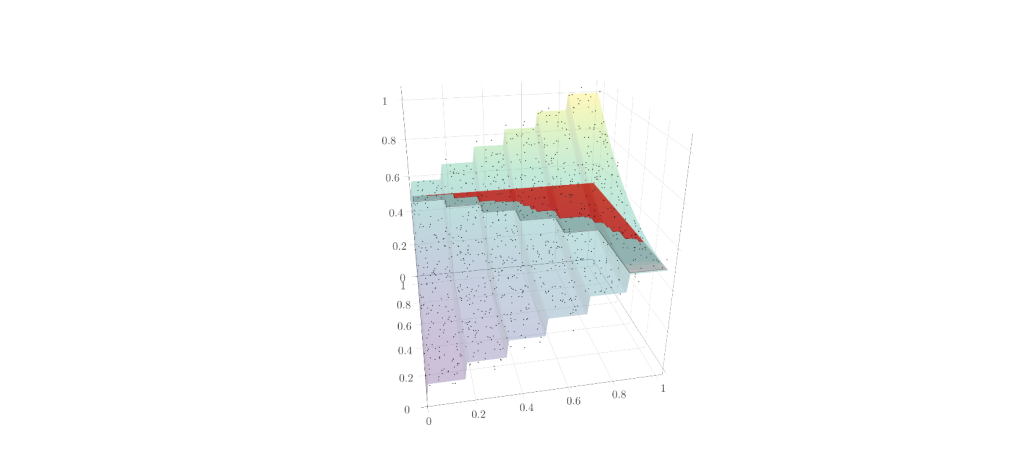
Figure 1: A visualisation with $d=2$ and $n=1000$. The unknown regression function is $(x^{(1)},x^{(2)})^{\top}\mapsto\lceil 6x^{(1)}\rceil/6+\bigl{(}x^{(2)}\bigr{)}^{2}$ rescaled to the interval $[0,1]$, depicted by the multi-coloured surface. The unknown grey surface gives the $0.5$-superlevel set, of which the red area is selected by our proposed procedure $\hat{A}^{\mathrm{ISS}}$.

One plausible strategy to achieve this goal is to construct a one-sided, uniform confidence band for $\eta$, and output the set on which the lower confidence limit is at least $\tau$. Unfortunately, however, such an approach tends to have sub-optimal empirical performance (see Section 5), because the lower confidence bound is required to protect against exceeding $\eta(x)$ at all points $x$ in the covariate domain, whereas it is only points close to the boundary of the $\tau$-superlevel set for which there is significant doubt about their inclusion. We therefore adopt a different approach, and seek to compute at each observation a $p$-value for the null hypothesis that the regression function is below $\tau$ based on an anytime-valid martingale procedure (Duan et al.,, 2020; Howard et al.,, 2021). The monotonicity of the regression function implies logical relationships between these hypotheses, but it is far from obvious how to combine the $p$-values effectively, particularly in the multivariate case, where we do not have a natural total ordering on $\mathbb{R}^{d}$. Our strategy is to introduce a tailored multiple testing procedure with familywise error rate control, building on ideas of Goeman and Solari, (2010) and Meijer and Goeman, (2015). This allows us to construct our final output set $\hat{A}^{\mathrm{ISS}}$ as the upper hull of the observations corresponding to the rejected hypotheses; see Section 2 for a more formal description of our proposed procedure, which is both computationally feasible and does not require the choice of any smoothing parameters. Our methodology is implemented in the R package ISS (Müller et al.,, 2023); an illustration in a bivariate example is given in Figure 1.

Our first theoretical result, in Section 3.1, verifies that $\hat{A}^{\mathrm{ISS}}$ does indeed control Type I error in the sense outlined above. We then turn our attention to power in Section 3.2, and provide both high-probability and expectation bounds on $\mu\bigl{(}\mathcal{X}_{\tau}(\eta)\setminus\hat{A}^{\mathrm{ISS}}\bigr{)}$. Our bound decomposes as a sum of two terms, where the first reflects the error incurred in determining whether each data point belongs to $\mathcal{X}_{\tau}(\eta)$, and depends on the growth rate of the regression function as we move further into the $\tau$-superlevel set from its boundary. The second term represents the error arising from the uncertainty of whether or not regions between the data points belong to this superlevel set. Our final theoretical contribution, in Section 3.3, reveals that $\hat{A}^{\mathrm{ISS}}$ attains the optimal power in the sense of minimising $\mathbb{E}\bigl{\{}\mu\bigl{(}\mathcal{X}_{\tau}(\eta)\setminus\hat{A}^{\mathrm{ISS}}\bigr{)}\bigr{\}}$ up to poly-logarithmic factors, among all procedures that control the Type I error.

In Section 4, we present various extensions that broaden the scope of our methodology. First, in Section 4.1, we describe alternative $p$-values that can be used, and that may yield more power for small and moderate sample sizes. Section 4.2 introduces three variants of $\hat{A}^{\mathrm{ISS}}$ that are tailored to specific settings including Gaussian errors, classification and heavy-tailed errors. Finally, in Section 4.3, we show how our proposal can be extended to cover heterogeneous treatment effect settings.

Section 5 is devoted to a study of the empirical performance of $\hat{A}^{\mathrm{ISS}}$ in a wide range of settings, with 14 regression functions chosen to illustrate different characteristics of interest, as well as different sample sizes and dimensions. The broad conclusion across these many scenarios is that, compared with various alternative approaches, $\hat{A}^{\mathrm{ISS}}$ has the most power for isotonic subgroup selection. In Section 6, we illustrate the performance of $\hat{A}^{\mathrm{ISS}}$ on two real datasets, the first of which is taken from the AIDS Clinical Trials Group Study 175 (ACTG 175) (Juraska et al.,, 2022). Here, we consider two problems: first, we seek to identify a low-risk subgroup and, second, in the context of heterogeneous treatment effects, we aim to identify a subgroup of patients for whom a new therapy is at least as effective as the baseline medication. The second dataset concerns fuel consumption (Quinlan,, 1993), where we seek to identify fuel-efficient cars based on their weight and engine displacement. The appendix consists of proofs of all of our main results, as well as statements and proofs of auxiliary results, further simulations and a discussion of an alternative and general approach to combining the $p$-values due to Meijer and Goeman, (2015). Although this strategy is often highly effective in multiple testing problems, we show that, surprisingly, it has sub-optimal worst-case performance in our isotonic subgroup selection setting.

Isotonic regression has a long history dating back to Ayer et al., (1955), Brunk, (1955) and van Eeden, (1956). Much recent interest has focused on risk bounds and oracle inequalities, which have been derived by Meyer and Woodroofe, (2000), Zhang, (2002), Chatterjee, (2014), Chatterjee et al., (2015), Bellec, (2018), Han et al., (2019), Deng and Zhang, (2020), Fokianos et al., (2020) and Pananjady and Samworth, (2022). Pointwise asymptotic confidence intervals in multivariate isotonic regression have been proposed by Deng et al., (2021), while confidence bands in the univariate case have been studied by Yang and Barber, (2019).

In the clinical trials community, the dangers of the naive approach to subgroup selection that ignores the key post-selection inference issue have been well understood for many years (Senn and Harrell,, 1997; Feinstein,, 1998; Rothwell,, 2005; Wang et al.,, 2007; Kaufman and MacLehose,, 2013; Altman,, 2015; Zhang et al.,, 2015; Gabler et al.,, 2016; Lipkovich et al.,, 2017; Watson and Holmes,, 2020). Valid approaches that control Type I error in the sense above have been proposed by Ballarini et al., (2018) and Wan et al., (2022) in the context of linear regression, and Reeve et al., (2021) for a smoothly-varying regression function.

The asymmetry of the two losses in our framework has some similarities with that of Neyman–Pearson classification (Cannon et al.,, 2002; Scott and Nowak,, 2005; Tong et al.,, 2016; Xia et al.,, 2021). There, covariate-response pairs $(X,Y)$ take values in $\mathbb{R}^{d}\times\{0,1\}$, and we seek a classifier $C:\mathbb{R}^{d}\rightarrow\{0,1\}$ that minimises $\mathbb{P}\bigl{(}C(X)=0|Y=1\bigr{)}$ subject to an upper bound on $\mathbb{P}\bigl{(}C(X)=1|Y=0\bigr{)}$. In addition to allowing continuous responses, another key difference of our paradigm is that we incur a Type I error whenever our selected set $\hat{A}$ contains a single point that does not belong to the $\tau$-superlevel set of the regression function. In other words, instead of controlling averages over sub-populations, our framework provides guarantees at an individual level, which is ethically advantageous, e.g. in medical contexts.

To conclude the introduction, we collect some notation used throughout the paper.

Notation.

For $n\in\mathbb{N}$, let $[n]:=\{1,\ldots,n\}$ and let $[0]:=\emptyset$. Write $x\wedge y:=\min(x,y)$ and $x\vee y:=\max(x,y)$ for $x,y\in\mathbb{R}$. Further, let $x_{+}:=x\vee 0$ and $\log_{+}x:=\log(x\vee e)$ for $x\in\mathbb{R}$. Denote by $\|\cdot\|_{\infty}$ the supremum norm on $\mathbb{R}^{d}$, and given $x\in\mathbb{R}^{d}$ and $r>0$, define the closed supremum norm ball by ${B}_{\infty}(x,r):=\{z\in\mathbb{R}^{d}:\|z-x\|_{\infty}\leq r\}$. For $x_{1}=(x_{1}^{(1)},\ldots,x_{1}^{(d)})^{\top},x_{2}=(x_{2}^{(1)},\ldots,x_{2}^{(d)})^{\top}\in\mathbb{R}^{d}$, we write $x_{1}\preccurlyeq x_{2}$ (or, equivalently, $x_{2}\succcurlyeq x_{1}$) if $x_{1}^{(j)}\leq x_{2}^{(j)}$ for all $j\in[d]$. A function $f:\mathbb{R}^{d}\rightarrow\mathbb{R}$ is said to be (coordinate-wise) increasing if $f(x_{0})\leq f(x_{1})$ whenever $x_{0}\preccurlyeq x_{1}$. A set $U\subseteq\mathbb{R}^{d}$ is called an upper set if, whenever $x\in U$ and $x\preccurlyeq x^{\prime}$, we have $x^{\prime}\in U$. Given $A\subseteq\mathbb{R}^{d}$, the upper hull of $A$ is the intersection of all upper sets that contain $A$. For a Borel probability measure $\mu$ on $\mathbb{R}^{d}$, we let $\mathrm{supp}(\mu)$ denote the support of $\mu$, i.e., the intersection of all closed sets $C\subseteq\mathbb{R}^{d}$ with $\mu(C)=1$. For $\tau\in\mathbb{R}$ and $f:\mathbb{R}^{d}\rightarrow\mathbb{R}$, we let $\mathcal{X}_{\tau}(f):=\{x\in\mathbb{R}^{d}:f(x)\geq\tau\}$.

A graph $G=(I,E)$ consists of a non-empty, finite set $I$ of vertices and a set $E\subseteq I\times I$ of edges. We say $G$ is directed if $(i,j)\in E$ does not imply $(j,i)\in E$. A directed path from $i\in I$ to $j\in I$ is a collection of distinct vertices $i_{0},i_{1},\ldots,i_{m}\in I$ for some $m\in\mathbb{N}$ with $i_{0}=i$ and $i_{m}=j$ such that $(i_{k-1},i_{k})\in E$ for all $k\in[m]$. A cycle is a directed path from $i\in I$ to itself. A directed acyclic graph (DAG) is a directed graph that does not contain any cycles. Given a DAG $G=(I,E)$, we write $L(G):=\{i\in I:(i,i^{\prime})\notin E\text{ for all }i^{\prime}\in I\}$ for the set of its leaf nodes and $\{i\in I:(i^{\prime},i)\notin E\text{ for all }i^{\prime}\in I\}$ for its root nodes. For $i\in I$, let $\operatorname{\mathrm{pa}}_{G}(i):=\{i^{\prime}\in I:(i^{\prime},i)\in E\}$ denote the set of parents of node $i$ and, similarly, write $\operatorname{\mathrm{ch}}_{G}(i):=\{i^{\prime}\in I:i\in\operatorname{\mathrm{pa}}_{G}(i^{\prime})\}$ for the set of children of node $i$. Further, defining $\operatorname{\mathrm{an}}^{1}_{G}(i):=\operatorname{\mathrm{pa}}_{G}(i)$ and $\operatorname{\mathrm{an}}^{k+1}_{G}(i):=\bigcup_{j\in\operatorname{\mathrm{an}}^{k}_{G}(i)}\operatorname{\mathrm{pa}}_{G}(j)$ for $k\in\mathbb{N}$, we can define $\operatorname{\mathrm{an}}_{G}(i):=\bigcup_{k\in\mathbb{N}}\operatorname{\mathrm{an}}^{k}_{G}(i)$ to be the set of ancestors of node $i$. Similarly, let $\operatorname{\mathrm{de}}_{G}(i):=\{i^{\prime}\in I:i\in\operatorname{\mathrm{an}}_{G}(i^{\prime})\}$ denote the set of descendants of node $i$. A reverse topological ordering of a DAG $G=(I,E)$ with $I=[m]$ is a permutation $\pi_{G}:I\rightarrow I$ such that if $i\in I$ and $i^{\prime}\in\operatorname{\mathrm{an}}_{G}(i)$, then $\pi_{G}(i)<\pi_{G}(i^{\prime})$. Any directed graph is acyclic if and only if it has a reverse topological ordering. We remark that all of these definitions remain unchanged when applied to a weighted DAG $G=(I,E,\bm{w})$, i.e. a DAG $(I,E)$ equipped with edge weights $\bm{w}=(w_{e}\geq 0:e\in E)$, and that any unweighted DAG may implicitly be assumed to be a weighted DAG with unit weights. A DAG $G=(I,E)$ is a polyforest if $|\operatorname{\mathrm{pa}}_{G}(i)|\leq 1$ for all $i\in I$, and a weighted DAG $G=(I,E,\bm{w})$ is a polyforest-weighted DAG if $F:=(I,\{e\in E:w_{e}>0\})$ is a polyforest.

2 Methodology

Let $P$ denote a distribution on $\mathbb{R}^{d}\times\mathbb{R}$, and let $(X,Y)\sim P$. Suppose that the regression function $\eta:\mathbb{R}^{d}\rightarrow\mathbb{R}$, defined by $\eta(x):=\mathbb{E}(Y|X=x)$, is increasing, and that the conditional distribution of $Y-\eta(X)$ given $X$ is sub-Gaussian with variance parameter $\sigma^{2}$. Given an independent and identically distributed sample $(X_{1},Y_{1}),\ldots,(X_{n},Y_{n})\sim P$, a threshold $\tau\in\mathbb{R}$ and a nominal Type I error rate $\alpha\in(0,1)$, we would like to identify a Borel measurable set $\hat{A}\subseteq\mathbb{R}^{d}$ such that with probability at least $1-\alpha$, we have $\eta(x)\geq\tau$ for all $x\in\hat{A}$. Subject to this constraint, we would like $\mu(\hat{A})$ to be as large as possible, where $\mu$ denotes the marginal distribution of $X$. An important observation is that, since $\mathcal{X}_{\tau}(\eta)$ is an upper set, replacing $\hat{A}$ with its upper hull does not increase the Type I error probability, and may increase its $\mu$-measure.

Our general strategy is initially to focus on a subset of observations, and seek to compute a $p$-value at each of these observations for the null hypothesis that the regression function is below $\tau$. We can then carefully combine these $p$-values using a multiple testing procedure having familywise error rate control over our structured hypotheses, and finally output the upper hull of the covariate observations corresponding to the rejected hypotheses. More precisely, for $m\in[n]$, and writing $\mathcal{D}_{X,m}:=(X_{1},\ldots,X_{m})$ for our reduced sample with the shorthand $\mathcal{D}_{X}:=\mathcal{D}_{X,n}$, we will construct $p$-values $\bm{p}:=(p_{i})_{i\in[m]}$ having the property that $\mathbb{P}(p_{i}\leq t|\mathcal{D}_{X})\leq t$ for every $t\in[0,1]$ whenever $\eta(X_{i})<\tau$. Next, we show how to exploit these $p$-values to obtain a set $\mathcal{R}_{\alpha}(\mathcal{D}_{X,m},\bm{p})\subseteq[m]$ of rejected hypotheses having the familywise error control property that with probability at least $1-\alpha$, we have $\eta(X_{i})\geq\tau$ for every $i\in\mathcal{R}_{\alpha}(\mathcal{D}_{X,m},\bm{p})$. Our final output set, $\hat{A}$, is the upper hull of $\{X_{i}:i\in\mathcal{R}_{\alpha}(\mathcal{D}_{X,m},\bm{p})\}$.

It remains to describe how we propose to construct the $p$-values, and to control the familywise error, and to this end, we first focus on the case $d=1$ for simplicity of exposition. One difference between the univariate and multivariate cases is that we take $m=n$ in the former. Consider the null hypothesis that $\eta(x)<\tau$ for some $x\in\mathbb{R}$, so that $\eta(X_{i})<\tau$ whenever $X_{i}\leq x$. Write $\mathcal{I}(x):=\{i\in[n]:X_{i}\leq x\}$ and $n(x):=|\mathcal{I}(x)|$, and, for $j\in[n(x)]$, let $X_{(j)}(x)$ denote the $j$th nearest neighbour of $x$ among $\{X_{i}:i\in\mathcal{I}(x)\}$, where for definiteness ties are broken by retaining the original ordering. Writing $Y_{(1)}(x),\ldots,Y_{(n)}(x)$ for the concomitant responses, under the null and conditional on $\mathcal{D}_{X}$, the process

$$S_{k}\equiv S_{k}(x,\sigma,\tau,\mathcal{D}):=\sum_{j=1}^{k}\frac{Y_{(j)}(x)-\tau}{\sigma}$$ (1)

for $k\in[n(x)]$ is a supermartingale with negative mean. Thus, large values of $S_{k}$ for some $k\in[n(x)]$ provide evidence against the null. One could also consider the alternative supermartingale $S_{k}^{\prime}:=\sum_{j=1}^{k}\bigl{(}Y_{(n(x)+1-j)}(x)-\tau\bigr{)}/\sigma$ for $k\in[n(x)]$, but our approach has the advantage that $S_{k}$ stochastically dominates $S_{k}^{\prime}$, so will have at least the same power. Tests based on supermartingales such as $(S_{k})$ are known as martingale tests (Duan et al.,, 2020) and time-uniform upper boundaries $(v_{k})$ are known for a variety of families of increment distributions (Howard et al.,, 2021); thus, $v_{k}\equiv v_{k}(\alpha)$ has the property that $\mathbb{P}\bigl{(}\max_{k\in[n(x)]}(S_{k}-v_{k})\geq 0\bigr{)}\leq\alpha$ under the null hypothesis $\eta(x)<\tau$. These inequalities can be inverted to yield a $p$-value; see Figure 2. Definition 1 below extends these ideas to the general multivariate case.

Figure 2: A schematic illustration of the proposed martingale test with $d=1$ and $\sigma=1$. Left: Raw data, where we denote $Z_{j}:=\bigl{(}X_{(j)}(x),Y_{(j)}(x)\bigr{)}$ and $\Delta_{j}:=Y_{(j)}(x)-\tau$ for $j\in[n(x)]$; note that the illustrated point $Z_{0}$ does not enter the martingale because its first component exceeds $x$. Right: The martingale $(S_{k})$, where $\bigl{(}v_{k}(\alpha)\bigr{)}_{k\in[n(x)]}$ denotes a suitable time-uniform upper boundary; here, $S_{4}\geq v_{4}(\alpha)$, so we would reject the null hypothesis $\eta(x)<\tau$ with a $p$-value satisfying $v_{4}(p)=S_{4}$.

Turning now to familywise error rate (FWER) control, and working conditional on $\mathcal{D}_{X}$ with $d=1$, consider $p$-values $\bm{p}:=(p_{i})_{i\in[n]}$ constructed as above for testing the null hypotheses $H_{i}:\eta(X_{i})<\tau$ for $i\in[n]$. One approach to controlling the FWER at level $\alpha$ is to reject only hypotheses $H_{i}$ with $i\in\mathcal{R}^{\mathrm{FS}}_{\alpha}(\mathcal{D}_{X},\bm{p})$, where

$$\mathcal{R}^{\mathrm{FS}}_{\alpha}(\mathcal{D}_{X},\bm{p}):=\{j\in[n]\!:\!p_{k}\leq\alpha\text{ for all }k\text{ with either }X_{k}>X_{j}\text{ or both }X_{k}=X_{j}\text{ and }k\leq j\}.$$

Controlling the FWER by employing an a priori ordering is known as a fixed sequence procedure (Westfall and Krishen,, 2001; Hsu and Berger,, 1999), and explains the superscript $\mathrm{FS}$ in the notation $\mathcal{R}^{\mathrm{FS}}_{\alpha}(\mathcal{D}_{X},\bm{p})$. Writing $H_{(i)}:\eta\bigl{(}X_{(i)}(\max_{j\in[n]}X_{j})\bigr{)}<\tau$ and $p_{(i)}$ for the corresponding $p$-value, this approach can be seen as a sequential procedure that, starting with $i=1$, stops and does not reject $H_{(i)}$ if $p_{(i)}>\alpha$ and otherwise rejects $H_{(i)}$ before proceeding to $i+1$, where the step is repeated. Here, the order in which we decide whether hypotheses should be rejected is motivated by the fact that $H_{(i)}\subseteq H_{(i+1)}$ for $i\in[n-1]$. A computationally-efficient implementation of this procedure only needs to calculate $p_{(i+1)}$ if $H_{(i)}$ has been rejected.

We now extend the presented ideas to the general case $d\in\mathbb{N}$. The construction of the $p$-values follows a similar approach as above, but the order in which the responses enter the supermartingale sequence is now determined by the supremum norm distance of the corresponding covariates from $x$.

Definition 1.

Given $x\in\mathbb{R}^{d}$, $\tau\in\mathbb{R}$, $\sigma>0$ and $\mathcal{D}=\bigl{(}(X_{1},Y_{1}),\ldots,(X_{n},Y_{n})\bigr{)}\in(\mathbb{R}^{d}\times\mathbb{R})^{n}$ write $\mathcal{I}(x)\equiv\mathcal{I}(x,\mathcal{D}_{X}):=\{i\in[n]:X_{i}\preccurlyeq x\}$ and again $n(x)\equiv n(x,\mathcal{D}_{X}):=|\mathcal{I}(x,\mathcal{D}_{X})|$. Further, for $j\in[n(x)]$, let $X_{(j)}(x)$ denote the $j$th nearest neighbour in $\{X_{i}:i\in\mathcal{I}(x)\}$ of $x$ in supremum norm, with ties broken by retaining the original ordering of the indices, and let $Y_{(1)}(x),\ldots,Y_{(n(x))}(x)$ denote the concomitant responses. Defining $S_{k}\equiv S_{k}(x,\sigma,\tau,\mathcal{D})$ for $k\in[n(x)]$ as in (1), we then set

$$\hat{p}_{\sigma,\tau}(x)\equiv\hat{p}_{\sigma,\tau}(x,\mathcal{D}):=1\wedge\min_{k\in[n(x)]}5.2\exp\biggl{\{}-\frac{(S_{k}\vee 0)^{2}}{2.0808k}+\frac{\log\log(2k)}{0.72}\biggr{\}},$$

whenever $n(x)>0$, and $\hat{p}_{\sigma,\tau}(x,\mathcal{D}):=1$ otherwise.

Lemma 5 below shows that $\hat{p}_{\sigma,\tau}(x,\mathcal{D})$ is indeed a $p$-value for the null hypothesis $\eta(x)<\tau$. We now proceed to the issue of FWER control in the multivariate setting, where we again condition on $\mathcal{D}_{X}$. Recall that we are interested in testing the hypotheses $H_{i}:\eta(X_{i})<\tau$ for $i\in[m]$ and a pre-specified $m\in[n]$. The fact that $\preccurlyeq$ induces only a partial order on $\mathbb{R}^{d}$ when $d>1$ means that there is no natural generalisation of the univariate fixed sequence testing procedure. Instead, we structure the hypotheses in a directed acyclic graph (DAG), with the edges in the graph representing logical relationships between hypotheses; such an approach has been studied in the literature to control both the FWER (Meijer and Goeman,, 2015) and the false discovery rate (Ramdas et al.,, 2019). The following definitions will be useful in the construction of an efficient multiple testing procedure.

Definition 2 (Induced DAGs and polyforests).

Let $\bm{z}=(z_{1},\ldots,z_{m})\in(\mathbb{R}^{d})^{m}$.

1. The induced DAG $\mathcal{G}(\bm{z})=\bigl{(}[m],\mathcal{E}(\bm{z})\bigr{)}$ is the graph with nodes $[m]$ and edges

   $$\mathcal{E}(\bm{z}):=\bigl{\{}(i_{0},i_{1})\in[m]^{2}:i_{0} \neq i_{1}\text{ and }z_{i_{1}}\preccurlyeq z_{i_{0}}\text{, and if }z_{i_{1}}\preccurlyeq z_{i_{2}}\preccurlyeq z_{i_{0}}\text{ then either }$$

   $$z_{i_{2}} =z_{i_{0}}\text{ and }i_{0}\leq i_{2}\text{, or }z_{i_{2}}=z_{i_{1}}\text{ and }i_{2}\leq i_{1}\bigr{\}}.$$

2. The induced polyforest $\mathcal{G}_{\mathrm{F}}(\bm{z})=\bigl{(}[m],\mathcal{E}_{\mathrm{F}}(\bm{z})\bigr{)}$ is the subgraph of $\mathcal{G}(\bm{z})$ with nodes $[m]$ and edges

   $$\mathcal{E}_{\mathrm{F}}(\bm{z}):=\Bigl{\{}(i_{0},i_{1})\in\mathcal{E}(\bm{z}):i_{0}=\operatorname*{sargmin}_{i:(i,i_{1})\in\mathcal{E}(\bm{z})}\|X_{i}-X_{i_{1}}\|_{\infty}\Bigr{\}}.$$

3. The induced polyforest-weighted DAG is $\mathcal{G}_{\mathrm{W}}(\bm{z}):=\bigl{(}[m],\mathcal{E}(\bm{z}),\bm{w}(\bm{z})\bigr{)}$, where $\bm{w}(\bm{z})=(w_{e})_{e\in\mathcal{E}(\bm{z})}$ is given by $w_{e}:=\mathbbm{1}_{\{e\in\mathcal{E}_{\mathrm{F}}(\bm{z})\}}$.

From the definition, we see that the induced polyforest-weighted DAG encodes the complete information of both $\mathcal{G}(\bm{z})$ and $\mathcal{G}_{\mathrm{F}}(\bm{z})$, as illustrated by Figure 3(a), where $d=2$ and each node represents the hypothesis corresponding to the observation at its location.

Definition 3 (DAG testing procedure).

A DAG testing procedure $\mathcal{R}$ is a function that takes as input a significance level $\alpha\in(0,1]$, a weighted DAG $G=(I,E,\bm{w})$ and $\bm{p}=(p_{i})_{i\in I}\in(0,1]^{I}$, and outputs a subset $\mathcal{R}_{\alpha}(G,\bm{p})\subseteq I$.

The fixed sequence procedure presented for $d=1$ is a DAG testing procedure since it only exploits the natural ordering information in $\mathcal{D}_{X}$, though in that case we wrote the first argument of $\mathcal{R}_{\alpha}^{\mathrm{FS}}$ as the set of nodes in the DAG rather than the full DAG for simplicity. In arbitrary dimensions, the methods proposed by Bretz et al., (2009), Meijer and Goeman, (2015) and Ramdas et al., (2019) are DAG testing procedures. While the Meijer and Goeman, (2015) procedure both controls the FWER and accounts for logical relationships between the hypotheses, theoretical and empirical power considerations lead us to propose a new approach that can be regarded as a sparsified version of the Meijer and Goeman, (2015) procedure or as an extension of the sequential rejection procedures of Bretz et al., (2009).

In order to describe our proposed iterative DAG testing procedure $\mathcal{R}^{\mathrm{ISS}}$, write $G:=\mathcal{G}(\mathcal{D}_{X,m})$ for the induced DAG and $F:=\mathcal{G}_{\mathrm{F}}(\mathcal{D}_{X,m})$ for the induced polyforest. We begin by splitting our $\alpha$-budget across the root nodes, with each such node receiving budget proportional to its number of leaf node descendants in $F$ (including the node itself if it is a leaf node). We reject each root node hypothesis whose $p$-value is at most its $\alpha$-budget, and whenever we do so, we also reject its ancestors in the original $G$ (which does not inflate the Type I error, due to the logical ordering of the hypotheses). The rejected root nodes are then removed from $F$, and we repeat the process iteratively, stopping when either we have rejected all hypotheses, or if we fail to reject any additional hypotheses at a given iteration. Formal pseudocode to compute $\mathcal{R}^{\mathrm{ISS}}$ is given in Algorithm 1; see also Figure 3 for an illustration.

(a) In the first iteration, no hypothesis has been rejected yet and only root nodes are assigned positive $\alpha$-budget. Here, nodes $1,6$ and $7$ are current rejection candidates, and $1$ will be rejected, as $p_{1}=0.01\leq 0.0125$.

(b) After rejection of node $1$ in the first step, we reallocate the $\alpha$-budget, which allows us to reject node $7$.

(c) Now that node $7$ has been rejected, its child $5$ receives $\alpha$-budget sufficiently large for it to be rejected. Although $p_{6}$ is quite large, $6$ is an ancestor of $5$ in the induced DAG and will hence also be rejected.

(d) None of the remaining three nodes, which happen to be the leaf nodes, have a $p$-value smaller than their respective $\alpha$-budgets. Hence, no further rejection is made and the procedure terminates. Nodes $1$, $5$, $6$ and $7$ have been rejected.

Figure 3: Illustration of Algorithm 1 with $\alpha=0.05$. Nodes are numbered according to one potential reverse topological ordering of the induced weighted DAG. The $p$-value for each hypothesis is given in round brackets. Solid arrows represent edges with weight $1$ in the induced polyforest-weighted DAG, whereas dashed arrows represent those with weight $0$. Each iteration of the procedure corresponds to one panel. A filled circle indicates that the hypothesis has been rejected in a previous step. If a node is assigned positive $\alpha$-budget at the current iteration, then its (rounded) budget is given in purple to the top left.

The DAG testing procedure $\mathcal{R}^{\mathrm{ISS}}$ allows us to define the corresponding isotonic subgroup selection set

$$\hat{A}^{\mathrm{ISS}}\equiv\hat{A}^{\mathrm{ISS}}_{\sigma,\tau,\alpha,m}(\mathcal{D}):=\bigl{\{}x\in\mathbb{R}^{d}:\!X_{i_{0}}\preccurlyeq x\text{ for some }i_{0}\in\mathcal{R}_{\alpha}^{\mathrm{ISS}}\bigl{(}\mathcal{G}_{\mathrm{W}}(\mathcal{D}_{X,m}),\bigl{(}\hat{p}_{\sigma,\tau}(X_{i},\mathcal{D})\bigr{)}_{i\in[m]}\bigr{)}\bigr{\}}.$$

Pseudocode for computing $\hat{A}^{\mathrm{ISS}}$ is given in Algorithm 2. In Section 3 below, we establish that $\hat{A}^{\mathrm{ISS}}$ controls the Type I error uniformly over appropriate distributional classes, and moreover has optimal worst-case power up to poly-logarithmic factors.

Input: $\alpha\in(0,1)$, polyforest-weighted DAG $(I,E,\bm{w})$, $\bm{p}=(p_{i})_{i\in I}\in(0,1]^{I}$

$G\leftarrow(I,E)$ // $G$ gives the logical structure of the hypotheses

$F\leftarrow(I,\{e\in E:w_{e}=1\})$ // $F$ determines the allocation of the $\alpha$-budget

$R_{0}\leftarrow\emptyset$

for $\ell\in[|I|]$ do

       $S_{\mathrm{L}}\leftarrow L(F)\setminus R_{\ell-1}$ // currently unrejected $F$-leaf nodes

       $S_{\mathrm{C}}\leftarrow\{i\in I:i\notin R_{\ell-1},\operatorname{\mathrm{pa}}_{F}(i)\subseteq R_{\ell-1}\}$ // current rejection candidates

       $\alpha_{i}\leftarrow\mathbbm{1}_{\{i\in S_{\mathrm{C}}\}}\cdot\bigl{|}\bigl{(}\{i\}\cup\operatorname{\mathrm{de}}_{F}(i)\bigr{)}\cap S_{\mathrm{L}}\bigr{|}\cdot\alpha/|S_{\mathrm{L}}|$ for all $i\in I$

       $I_{\ell}\leftarrow\{i\in I:p_{i}\leq\alpha_{i}\}$

       if $I_{\ell}=\emptyset$ then

             $R_{|I|}\leftarrow R_{\ell-1}$ // will not make any further rejections

             break

       $R_{\ell}\leftarrow R_{\ell-1}\cup I_{\ell}\cup\bigcup_{i\in I_{\ell}}\operatorname{\mathrm{an}}_{G}(i)$ // reject $I_{\ell}$ and its ancestors in $G$

       if $R_{\ell}=I$ then

             $R_{|I|}\leftarrow R_{\ell}$ // everything has been rejected

             break

      

end for

Result: The set of rejected hypotheses $\mathcal{R}_{\alpha}^{\mathrm{ISS}}\bigl{(}(I,E,\bm{w}),\bm{p}\bigr{)}:=R_{|I|}$

Algorithm 1 The DAG testing procedure $\mathcal{R}^{\mathrm{ISS}}$.

Input: $\mathcal{D}=(X_{i},Y_{i})_{i\in[n]}\in(\mathbb{R}^{d}\times\mathbb{R})^{n}$, $\tau\in\mathbb{R}$, $\alpha\in(0,1)$, $\sigma>0$, $m\in[n]$

$\mathcal{D}_{X,m}\leftarrow(X_{1},\ldots,X_{m})$ // subsample the first $m$ covariate points in $\mathcal{D}$

$p_{i}\leftarrow\hat{p}_{\sigma,\tau}(X_{i})$ for $i\in[m]$ // calculate $p$-values as in Definition 1

$G\leftarrow\mathcal{G}_{\mathrm{W}}(\mathcal{D}_{X,m})$ // construct induced polyforest-weighted DAG

$R\leftarrow\mathcal{R}^{\mathrm{ISS}}_{\alpha}\bigl{(}G,(p_{1},\ldots,p_{m})\bigr{)}$ // combine $p$-values via Algorithm 1

$\hat{A}^{\mathrm{ISS}}_{\sigma,\tau,\alpha,m}(\mathcal{D})\leftarrow\{x\in\mathbb{R}^{d}:X_{i}\preccurlyeq x\text{ for some }i\in R\}$ // select upper hull of $(X_{i})_{i\in R}$

Result: The selected set $\hat{A}^{\mathrm{ISS}}_{\sigma,\tau,\alpha,m}(\mathcal{D})$.

Algorithm 2 The subgroup selection algorithm $\hat{A}^{\mathrm{ISS}}$.

3 Theory

3.1 Type I error control

We first introduce the class of distributions over which we prove the Type I error control of $\hat{A}^{\mathrm{ISS}}$.

Definition 4.

Given $\sigma>0$, let $\mathcal{P}_{\mathrm{Mon},d}(\sigma)$ denote the class of all distributions $P$ on $\mathbb{R}^{d}\times\mathbb{R}$ with increasing regression function $\eta:\mathbb{R}^{d}\rightarrow\mathbb{R}$, and for which, when $(X,Y)\sim P$, the conditional distribution of $Y-\eta(X)$ given $X$ is sub-Gaussian with variance parameter $\sigma^{2}$.

Our Type I error control relies on showing first that $\hat{p}_{\sigma,\tau}(x,\mathcal{D})$ is indeed a $p$-value for testing the null hypothesis $\eta(x)<\tau$ when $P\in\mathcal{P}_{\mathrm{Mon},d}(\sigma)$ and then that the DAG testing procedure $\mathcal{R}^{\mathrm{ISS}}$ controls the FWER in the sense defined in Definition 7 below. The next lemma accomplishes the first of these tasks (in fact, it shows that $\hat{p}_{\sigma,\tau}(x,\mathcal{D})$ is a $p$-value even conditional on $\mathcal{D}_{X}$). We write $P^{n}$ for the $n$-fold product measure corresponding to $P$.

Lemma 5.

Given any $x\in\mathbb{R}^{d}$, $\tau\in\mathbb{R}$, $\sigma>0$, $P\in\mathcal{P}_{\mathrm{Mon},d}(\sigma)$ such that $\eta(x)<\tau$ and $\mathcal{D}=\bigl{(}(X_{1},Y_{1}),\ldots,(X_{n},Y_{n})\bigr{)}\sim P^{n}$, we have $\mathbb{P}_{P}\bigl{\{}\hat{p}_{\sigma,\tau}(x,\mathcal{D})\leq\alpha|\mathcal{D}_{X}\bigr{\}}\leq\alpha$ for all $\alpha\in(0,1)$.

We now direct our attention towards the DAG testing procedure $\mathcal{R}^{\mathrm{ISS}}$. Here, it is convenient to introduce the following terminology.

Definition 6.

Given a weighted, directed graph $G=(I,E,\bm{w})$, we say that a subset $I_{0}\subseteq I$ is $G$-lower if whenever $i_{0}\in I_{0}$ we have $\operatorname{\mathrm{de}}_{G}(i_{0})\subseteq I_{0}$. Conversely, $I_{0}\subseteq I$ is called $G$-upper if $I\setminus I_{0}$ is $G$-lower.

Given a finite set $I$, a family of distributions $\mathcal{Q}$ on $(0,1]^{I}$ and a finite collection of null hypotheses $H_{i}\subseteq\mathcal{Q}$ for $i\in I$, let $G_{0}:=(I,E_{0})$ with $E_{0}:=\{(i_{0},i_{1})\in I^{2}:H_{i_{0}}\subseteq H_{i_{1}}\}$ be the directed graph that encodes all logical relationships between hypotheses. Then for any $Q\in\mathcal{Q}$, the true null index set $I_{0}(Q):=\{i\in I:Q\in H_{i}\}$ is necessarily a $G_{0}$-lower set. Conversely, the index set of false null hypotheses must be a $G_{0}$-upper set. We say that a polyforest-weighted DAG $(I,E,\bm{w})$ is $G_{0}$-consistent if $E\subseteq E_{0}$. Multiple testing procedures that reject hypotheses corresponding to a $G_{0}$-upper set are called coherent (Gabriel,, 1969, p. 229), and by construction, $\mathcal{R}^{\mathrm{ISS}}$ is indeed coherent when applied to a $G_{0}$-consistent polyforest-weighted DAG.

We are now in a position to formalise the concept of FWER control for DAG testing procedures.

Definition 7.

A DAG testing procedure $\mathcal{R}$ controls the FWER if given any finite set $I$, a family of distributions $\mathcal{Q}$ on $(0,1]^{I}$, a collection of random variables $\bm{p}=(p_{i})_{i\in I}$ taking values in $(0,1]^{I}$, as well as hypotheses $H_{i}\subseteq\{Q\in\mathcal{Q}:\mathbb{P}_{Q}(p_{i}\leq t)\leq t,\forall t\in(0,1]\}$ for $i\in I$ and any $G_{0}$-consistent polyforest-weighted DAG $G^{\prime}=(I,E,\bm{w})$, we have $\mathbb{P}_{Q}\bigl{(}\mathcal{R}_{\alpha}(G^{\prime},\bm{p})\cap I_{0}(Q)\neq\emptyset\bigr{)}\leq\alpha$ for all $\alpha\in(0,1)$ and $Q\in\mathcal{Q}$.

Lemma 8.

The DAG testing procedure $\mathcal{R}^{\mathrm{ISS}}$ defined by Algorithm 1 controls the FWER.

The strategy of the proof of Lemma 8 is based on ideas in the proof of Goeman and Solari, (2010, Theorem 1). Combining Lemmas 5 and 8 yields our Type I error guarantee:

Theorem 9.

For any $d\in\mathbb{N}$, $n\in\mathbb{N}$, $m\in[n]$, $\alpha\in(0,1)$, $\tau\in\mathbb{R}$, $\sigma>0$, and $P\in\mathcal{P}_{\mathrm{Mon},d}(\sigma)$, along with $\mathcal{D}=\bigl{(}(X_{1},Y_{1}),\ldots,(X_{n},Y_{n})\bigr{)}\sim P^{n}$, we have

$$\mathbb{P}_{P}\bigl{(}\hat{A}^{\mathrm{ISS}}_{\sigma,\tau,\alpha,m}(\mathcal{D})\subseteq\mathcal{X}_{\tau}(\eta)\bigm{|}\mathcal{D}_{X}\bigr{)}\geq 1-\alpha.$$

Let $\hat{\mathcal{A}}_{n}(\tau,\alpha,\mathcal{P})$ denote the family of data-dependent selection sets $\hat{A}$ (i.e. Borel measurable functions from $(\mathbb{R}^{d}\times\mathbb{R})^{n}$ to the set of Borel subsets of $\mathbb{R}^{d}$) that control the Type I error rate at level $\alpha\in(0,1)$ over the family $\mathcal{P}$ of distributions on $\mathbb{R}^{d}\times\mathbb{R}$. In other words, we write $\hat{A}\in\hat{\mathcal{A}}_{n}(\tau,\alpha,\mathcal{P})$ if

$$\mathbb{P}_{P}\bigl{(}\hat{A}(\mathcal{D})\subseteq\mathcal{X}_{\tau}(\eta)\bigr{)}\geq 1-\alpha$$ (2)

for all $P\in\mathcal{P}$ with $\mathcal{D}\sim P^{n}$. An immediate consequence of Theorem 9 is that $\hat{A}_{\sigma,\tau,\alpha,m}^{\mathrm{ISS}}\in\hat{\mathcal{A}}_{n}\bigl{(}\tau,\alpha,\mathcal{P}_{\mathrm{Mon},d}(\sigma)\bigr{)}$. In fact, an inspection of the proof of Theorem 9 (see also Lemma 25) reveals that $\hat{A}_{\sigma,\tau,\alpha,m}^{\mathrm{ISS}}$ controls the Type I error over a larger class. Indeed, writing $\mathcal{P}_{\mathrm{Upp},d}(\tau,\sigma)$ for the class of distributions of pairs $(X,Y)$ such that the $\tau$-superlevel set of the regression function $\eta:\mathbb{R}^{d}\rightarrow\mathbb{R}$ is an upper set and, again, the conditional distribution of $Y-\eta(X)$ given $X$ is sub-Gaussian with variance parameter $\sigma^{2}$, it follows from the proof that $\hat{A}^{\mathrm{ISS}}_{\sigma,\tau,\alpha,m}\in\hat{\mathcal{A}}_{n}\bigl{(}\tau,\alpha,\mathcal{P}_{\mathrm{Upp},d}(\tau,\sigma)\bigr{)}$. We have $\mathcal{P}_{\mathrm{Mon},d}(\sigma)=\bigcap_{\tau^{\prime}\in\mathbb{R}}\mathcal{P}_{\mathrm{Upp},d}(\tau^{\prime},\sigma)$, but the regression functions of distributions in $\mathcal{P}_{\mathrm{Upp},d}(\tau,\sigma)$ for a fixed $\tau\in\mathbb{R}$ may deviate from monotonicity as long as the $\tau$-superlevel set remains an upper set. In this sense, our procedure $\hat{A}_{\sigma,\tau,\alpha,m}^{\mathrm{ISS}}$ is robust to misspecification of the monotonicity of the regression function.

3.2 Power

Classical results on Gaussian testing reveal that merely asking for $P\in\mathcal{P}_{\mathrm{Mon},d}(\sigma)$ is insufficient to be able to provide non-trivial uniform power guarantees for data-dependent selection sets with Type I error control (see Proposition 26 in Appendix A.2 for details). The main issue here is that the marginal distribution $\mu$ may place a lot of mass in regions where $\eta$ is only slightly above $\tau$, and these regions will be hard for a data-dependent selection set to include if it has Type I error control. In this section, therefore, we introduce a margin condition that controls the $\mu$-measure of these difficult regions.

Definition 10.

For $d\in\mathbb{N}$, $\tau\in\mathbb{R}$, $\beta>0$ and $\nu>0$, let $\mathcal{P}_{\mathrm{Mar},d}(\tau,\beta,\nu)$ denote the class of distributions $P$ on $\mathbb{R}^{d}\times\mathbb{R}$ for which the marginal $\mu$ on $\mathbb{R}^{d}$ and the regression function $\eta:\mathbb{R}^{d}\rightarrow\mathbb{R}$ satisfy $\mu\bigl{(}\eta^{-1}([\tau,\tau+\nu\xi^{\beta}])\bigr{)}\leq\xi$ for all $\xi\in(0,1]$.

Example 1.

Let $d=1$ and let $P\in\mathcal{P}_{\mathrm{Mon},1}(\sigma)$ have uniform marginal distribution $\mu$ on $[0,1]$ and regression function $\eta$. We then have $P\in\mathcal{P}_{\mathrm{Mon},1}(\sigma)\cap\mathcal{P}_{\mathrm{Mar},1}(\tau,\beta,\nu)$ if $\eta(x+\xi)\geq\tau+\nu\xi^{\beta}$ for all $\xi\in(0,1]$ and $x\in\mathcal{X}_{\tau}(\eta)$.

We now divide our power analysis for $\hat{A}^{\mathrm{ISS}}$ into univariate and multivariate cases, since the natural total order on $\mathbb{R}$ means that our results simplify a little when $d=1$. Theorem 11 below provides high-probability and expectation upper bounds on the regret $\mu\bigl{(}\mathcal{X}_{\tau}(\eta)\setminus\hat{A}^{\mathrm{ISS}}\bigr{)}$ for $P\in\mathcal{P}_{\mathrm{Mon},1}(\sigma)\cap\mathcal{P}_{\mathrm{Mar},1}(\tau,\beta,\nu)$.

Theorem 11.

Let $\sigma,\beta,\nu>0$ and $\alpha\in(0,1)$. There exists a universal constant $C>0$ such that for any distribution $P\in\mathcal{P}_{\mathrm{Mon},1}(\sigma)\cap\mathcal{P}_{\mathrm{Mar},1}(\tau,\beta,\nu)$ and $\delta\in(0,1)$, we have

$$\mathbb{P}_{P}\biggl{[}\mu\bigl{(}\mathcal{X}_{\tau}(\eta)\setminus\hat{A}^{\mathrm{ISS}}_{\sigma,\tau,\alpha,n}(\mathcal{D})\bigr{)}>1\wedge C\biggl{\{}\biggl{(}\frac{\sigma^{2}}{n\nu^{2}}\log_{+}\Bigl{(}\frac{\log_{+}n}{\alpha\wedge\delta}\Bigr{)}\biggr{)}^{1/(2\beta+1)}+\frac{\log_{+}(1/\delta)}{n}\biggr{\}}\biggr{]}\leq\delta,$$

and

$$\mathbb{E}_{P}\bigl{\{}\mu\bigl{(}\mathcal{X}_{\tau}(\eta)\setminus\hat{A}^{\mathrm{ISS}}_{\sigma,\tau,\alpha,n}(\mathcal{D})\bigr{)}\bigr{\}}\leq 1\wedge C\biggl{\{}\biggl{(}\frac{\sigma^{2}}{n\nu^{2}}\log_{+}\Bigl{(}\frac{\log_{+}n}{\alpha}\Bigr{)}\biggr{)}^{1/(2\beta+1)}+\frac{1}{n}\biggr{\}}.$$

From Theorem 11, we see that the regret of $\hat{A}^{\mathrm{ISS}}$ decomposes as a sum of two terms: the first reflects the error incurred in determining whether each data point belongs to $\mathcal{X}_{\tau}(\eta)$, while the second represents the error arising from the uncertainty of whether or not regions between the data points belong to this superlevel set. The combination of Theorem 11 with Proposition 14 below and Theorem 17 in Section 3.3 reveals that the dependence of our bound on the parameters $n$, $\alpha$, $\sigma$, $\beta$ and $\nu$ is optimal up to an iterated logarithmic factor in $n$.

In the proof of Theorem 11, we exploit the fact that $\mathcal{D}_{X}$ has a total order in the univariate case, so the corresponding induced polyforest-weighted DAG forms a directed path in which each edge has weight $1$. Since in our algorithm, the $p$-values $\hat{p}_{\sigma,\tau}$ for coinciding hypotheses are equal, $\mathcal{R}^{\mathrm{ISS}}$ is equivalent to the fixed sequence procedure $\mathcal{R}^{\mathrm{FS}}$.

Turning now to the multivariate case, we begin with a negative result, which reveals that we can find distributions in our class for which no data-dependent selection set with Type I error control performs better than the trivial procedure that ignores the data, and selects the entire domain with probability $\alpha$ and the empty set otherwise.

Proposition 12.

Let $d\geq 2$, $\tau\in\mathbb{R}$, $\sigma,\beta,\nu>0$ and $\alpha\in(0,1)$. Then, writing $\mathcal{P}^{\prime}:=\mathcal{P}_{\mathrm{Mon},d}(\sigma)\cap\mathcal{P}_{\mathrm{Mar},d}(\tau,\beta,\nu)$, we have for any $n\in\mathbb{N}$ that

$$\sup_{P\in\mathcal{P}^{\prime}}\inf_{\hat{A}\in\hat{\mathcal{A}}_{n}(\tau,\alpha,\mathcal{P}^{\prime})}\mathbb{E}_{P}\bigl{\{}\mu\bigl{(}\mathcal{X}_{\tau}(\eta)\setminus\hat{A}(\mathcal{D})\bigr{)}\bigr{\}}\geq 1-\alpha.$$

An interesting feature of Proposition 12 is the ordering of the supremum over distributions in our class and the infimum over data-dependent selection sets. Usually, with minimax lower bounds, these would appear in the opposite order, but here we are able to establish the stronger conclusion, because it is the same subfamily of $\mathcal{P}_{\mathrm{Mon},d}(\sigma)\cap\mathcal{P}_{\mathrm{Mar},d}(\tau,\beta,\nu)$ that causes the poor performance of any data-dependent selection set with Type I error control. In fact, by examining the proof, we see that the issue is caused by constructing a marginal distribution $\mu$ that concentrates its mass around a large antichain in $[0,1]^{d}$, which constitutes the boundary of $\mathcal{X}_{\tau}(\eta)$. This motivates us to regulate the extent to which this is allowed to happen.

Definition 13.

Given $d\in\mathbb{N}$, $\tau\in\mathbb{R}$, $\theta>1$, $\gamma,\lambda>0$, we let $\mathcal{P}_{\mathrm{Reg},d}(\tau,\theta,\gamma,\lambda)$ denote the class of all distributions $P$ on $\mathbb{R}^{d}\times\mathbb{R}$ with marginal $\mu$ on $\mathbb{R}^{d}$ and associated regression function $\eta$ such that

1. $\theta^{-1}\cdot r^{d}\leq\mu\bigl{(}{B}_{\infty}(x,r)\bigr{)}\leq\theta\cdot(2r)^{d}$ for all $x\in\mathcal{X}_{\tau}(\eta)\cap\mathrm{supp}(\mu)$ and $r\in(0,1]$;

2. ${B}_{\infty}(x,r)\cap\mathcal{X}_{\tau+\lambda\cdot r^{\gamma}}(\eta)\neq\emptyset$ for all $x\in\mathcal{X}_{\tau}(\eta)\cap\mathrm{supp}(\mu)$ and $r\in(0,1]$.

For distributions in the $\mathcal{P}_{\mathrm{Mon},d}(\sigma)$ class, Definition 13 represents a slight strengthening of the margin condition used in our univariate analysis, as made precise by Proposition 14 below.

Proposition 14.

Let $d\in\mathbb{N}$, $\tau\in\mathbb{R}$, $\sigma,\gamma,\lambda>0$ and $\theta>1$. There exists $C\geq 1$, depending only on $(d,\theta)$, such that

$$\mathcal{P}_{\mathrm{Mon},d}(\sigma)\cap\mathcal{P}_{\mathrm{Reg},d}(\tau,\theta,\gamma,\lambda)\subseteq\mathcal{P}_{\mathrm{Mon},d}(\sigma)\cap\mathcal{P}_{\mathrm{Mar},d}(\tau,\gamma,\lambda/C^{\gamma}).$$

Thus, $(\gamma,\lambda)$ in the class $\mathcal{P}_{\mathrm{Reg},d}(\tau,\theta,\gamma,\lambda)$ play a similar but not identical role to $(\beta,\nu)$ in $\mathcal{P}_{\mathrm{Mar},d}(\tau,\beta,\nu)$, in controlling the way in which the regression function is required to grow as we move away from the boundary of the $\tau$-superlevel set. We are now in a position to state our main result concerning the power of our proposed procedure; the result holds in all dimensions but our primary interest here is in the multivariate case.

Theorem 15.

Let $d\in\mathbb{N}$, $\tau\in\mathbb{R}$, $\sigma,\gamma,\lambda>0$ and $\theta>1$. There exists $C\geq 1$, depending only on $(d,\theta)$, such that for any $P\in\mathcal{P}_{\mathrm{Mon},d}(\sigma)\cap\mathcal{P}_{\mathrm{Reg},d}(\tau,\theta,\gamma,\lambda)$, $n\in\mathbb{N}$, $\alpha\in(0,1)$ and $\delta\in(0,1)$, along with $\mathcal{D}=\bigl{(}(X_{1},Y_{1}),\ldots,(X_{n},Y_{n})\bigr{)}\sim P^{n}$, we have for $m\in[n]$ that

$$\mathbb{P}_{P}\biggl{[}\mu\bigl{(}\mathcal{X}_{\tau}(\eta)\setminus\hat{A}^{\mathrm{ISS}}_{\sigma,\tau,\alpha,m}(\mathcal{D})\bigr{)}>1\wedge C\biggl{\{}\biggl{(}\frac{\sigma^{2}}{n\lambda^{2}}\log_{+}\Bigl{(}\frac{m\log_{+}n}{\alpha\wedge\delta}\Bigr{)}\biggr{)}^{\frac{1}{2\gamma+d}}+\biggl{(}\frac{\log_{+}(m/\delta)}{m}\biggr{)}^{\frac{1}{d}}\biggr{\}}\biggr{]}\leq\delta,$$

and

$$\mathbb{E}_{P}\bigl{\{}\mu\bigl{(}\mathcal{X}_{\tau}(\eta)\setminus\hat{A}^{\mathrm{ISS}}_{\sigma,\tau,\alpha,m}(\mathcal{D})\bigr{)}\bigr{\}} \leq 1\wedge C\biggl{\{}\biggl{(}\frac{\sigma^{2}}{n\lambda^{2}}\log_{+}\Bigl{(}\frac{m\log_{+}n}{\alpha}\Bigr{)}\biggr{)}^{1/(2\gamma+d)}+\biggl{(}\frac{\log_{+}m}{m}\biggr{)}^{1/d}\biggr{\}}.$$

The terms in the bound in Theorem 15 are similar to those in Theorem 11, and exhibit the trade-off in the choice of $m$: if we choose it to be small, then there are fewer data points in our subsample that belong to $\mathcal{X}_{\tau}(\eta)$ and moreover these are less likely to be excluded from $\hat{A}^{\mathrm{ISS}}$ because they are typically assigned greater budget in our DAG testing procedure. On the other hand, we incur a greater loss in excluding regions between data points in our subsample that belong to this superlevel set. By specialising Theorem 15 via a particular choice of $m$, we obtain the following almost immediate corollary. It is this upper bound to which we will compare our minimax lower bound in Theorem 17.

Corollary 16.

Under the conditions of Theorem 15, if we take $m_{0}:=n\wedge\lceil n\lambda^{2}/\sigma^{2}\rceil$, then

$$\mathbb{E}_{P}\bigl{\{}\mu\bigl{(}\mathcal{X}_{\tau}(\eta)\setminus\hat{A}^{\mathrm{ISS}}_{\sigma,\tau,\alpha,m_{0}}(\mathcal{D})\bigr{)}\bigr{\}} \leq 1\wedge 4C\biggl{\{}\biggl{(}\frac{\sigma^{2}}{n\lambda^{2}}\log_{+}\Bigl{(}\frac{n\lambda^{2}\log_{+}n}{\sigma^{2}\alpha}\Bigr{)}\biggr{)}^{1/(2\gamma+d)}+\biggl{(}\frac{\log_{+}n}{n}\biggr{)}^{1/d}\biggr{\}}.$$

As is apparent from the proof of Corollary 16, a high-probability bound analogous to that in Theorem 15 also holds, but this is omitted for brevity. In practice, one can take $m=n$ (as we do in our simulations in Section 5), with a corresponding power bound obtained as a special case of Theorem 15. Corollary 16 suggests a curse of dimensionality effect in isotonic subgroup selection; this is confirmed as an essential price to pay by Theorem 17 below.

3.3 Main lower bound

In order to discuss the optimality of our data-dependent selection set $\hat{A}^{\mathrm{ISS}}$, we present a minimax lower bound that provides a benchmark on the regret that is achievable by any data-dependent selection set with Type I error control.

Theorem 17.

Let $d\in\mathbb{N}$, $\tau\in\mathbb{R}$, $\sigma,\gamma,\lambda>0$ and $\theta>1$. Then, writing $\mathcal{P}^{\prime}:=\mathcal{P}_{\mathrm{Mon},d}(\sigma)\cap\mathcal{P}_{\mathrm{Reg},d}(\tau,\theta,\gamma,\lambda)$, there exists $c\in(0,1)$, depending only on $(d,\gamma)$, such that for any $n\in\mathbb{N}$ and $\alpha\in(0,1/4]$, we have

$$\inf_{\hat{A}\in\hat{\mathcal{A}}_{n}(\tau,\alpha,\mathcal{P}^{\prime})}\sup_{P\in\mathcal{P}^{\prime}}\mathbb{E}_{P}\bigl{\{}\mu\bigl{(}\mathcal{X}_{\tau}(\eta)\setminus\hat{A}(\mathcal{D})\bigr{)}\bigr{\}}\geq c\biggl{[}1\wedge\biggl{\{}\biggl{(}\frac{\sigma^{2}}{n\lambda^{2}}\log_{+}\Bigl{(}\frac{1}{5\alpha}\Bigr{)}\biggr{)}^{1/(2\gamma+d)}+\frac{1}{n^{1/d}}\biggr{\}}\biggr{]}.$$ (3)

By comparing the rate in Theorem 17 with those in Theorem 11 and Corollary 16, we see that $\hat{A}^{\mathrm{ISS}}$ attains the optimal regret among procedures with Type I error control, up to poly-logarithmic factors. In particular, up to such factors, these results reveal the optimal dependence of the regret not only on $n$, but also on $\sigma$, $\lambda$ and $\alpha$. It is interesting to note that Theorem 17 incorporates procedures that are only required to control Type I error over $\mathcal{P}_{\mathrm{Mon},d}(\sigma)\cap\mathcal{P}_{\mathrm{Reg},d}(\tau,\theta,\gamma,\lambda)$, whereas $\hat{A}^{\mathrm{ISS}}$ has Type I error control over the larger class $\mathcal{P}_{\mathrm{Mon},d}(\sigma)$, by Theorem 9. Thus, $\hat{A}^{\mathrm{ISS}}$ suffers no deterioration in performance for this stronger validity guarantee, at least up to poly-logarithmic factors.

The proof of Theorem 17 combines two minimax lower bounds, given in Propositions 31 and 33, which provide the different terms in the sum in (3). The main idea in both cases is to divide $[0,1]^{d}$ into a hypercube lattice, and to construct pairs of distributions where either the regression function (Proposition 31) or the marginal distribution (Proposition 33) only differ in a single hypercube among a collection whose centres lie on a large antichain in $\mathbb{R}^{d}$. Observations outside these critical hypercubes therefore do not help to distinguish between the distributions in a pair, so by choosing the number of hypercubes and the difference in the regression function levels appropriately, we obtain a non-trivial probability of failing to include them in a data-dependent selection set. Our formal constructions, together with illustrations, are given in Section A.3.

4 Extensions

4.1 Choice of $p$-value construction

Recall that in our isotonic subgroup selection procedure $\hat{A}^{\mathrm{ISS}}$, we propose a $p$-value based on a martingale test in combination with a finite law of the iterated logarithm (LIL) bound (Lemma 45(a)). The following definition gives an alternative $p$-value construction that uses a different bound and includes a hyperparameter $\rho>0$.

Definition 18.

In the setting of Definition 1, for $\rho>0$, we define

$$\tilde{p}^{\rho}_{\sigma,\tau}(x)\equiv\tilde{p}^{\rho}_{\sigma,\tau}(x,\mathcal{D}):=1\wedge\min_{k\in[n(x)]}\sqrt{\frac{k+\rho}{4\rho}}\biggl{\{}\exp\biggl{(}\frac{(S_{k}\vee 0)^{2}}{2(k+\rho)}\biggr{)}-1\biggr{\}}^{-1}$$

whenever $n(x)>0$, and $\tilde{p}^{\rho}_{\sigma,\tau}(x,\mathcal{D}):=1$ otherwise.

By Lemma 45(b), which is due to Howard et al., (2021), in combination with the proof technique of Lemma 5, $\tilde{p}^{\rho}_{\sigma,\tau}(x)$ is indeed a $p$-value for the null hypothesis $\eta(x)<\tau$ (even conditional on $\mathcal{D}_{X}$). It follows that if we modify our procedure to use these $p$-values instead of those in Definition 1, then the Type I error guarantee in Theorem 9 is unaffected. The objective function being minimised over $k\in[n(x)]$ is a little smaller for the original $p$-value definition when $k$ is sufficiently large, and this therefore leads to a stronger power bound in Theorem 15. Nevertheless, for appropriate values of $\rho>0$, Definition 18 may yield a slightly smaller objective for small and moderate values of $k$, and hence may be preferable in practice. Based on some preliminary simulations, we found that the power of our approach varied very little over choices of $\rho\in(0,1]$, and that $\rho=1/2$ was a robust choice that we used throughout our experiments in Section 5 and recommend for practical use.

4.2 Alternative distributional assumptions

In this subsection, we introduce three variants of $\hat{A}^{\mathrm{ISS}}$, each of which is able to control Type I error over appropriate classes without knowledge of any nuisance parameter and without the need for sample splitting. In each case, we retain the same multiple testing component $\mathcal{R}^{\mathrm{ISS}}$ to our procedure, but construct the $p$-values in different ways. Power results analogous to Theorem 15 also hold for these versions of $\hat{A}^{\mathrm{ISS}}$, but are omitted for brevity.

4.2.1 Gaussian noise with unknown variance

Since Algorithm 2 takes the sub-Gaussian variance parameter $\sigma^{2}$ as an input, we present here an adaptive approach for a Gaussian error setting. More precisely, for $\sigma>0$, let $\mathcal{P}_{\mathrm{N},d}(\sigma)$ denote the subset of $\mathcal{P}_{\mathrm{Mon},d}(\sigma)$ with $Y-\eta(X)|X\sim\mathcal{N}(0,\sigma^{2})$.

Definition 19.

In the setting of Definition 1, let $\hat{\sigma}^{2}_{0,k}:=k^{-1}\sum_{j=1}^{k}\bigl{(}Y_{(j)}(x)-\tau\bigr{)}_{+}^{2}$ and $\bar{Y}_{1,k}:=k^{-1}\sum_{j=1}^{k}Y_{(j)}(x)$ for $k\in[n(x)]$ and $\hat{\sigma}^{2}_{1,k}:=k^{-1}\sum_{j=1}^{k}\bigl{(}Y_{(j)}(x)-\bar{Y}_{1,k}\bigr{)}^{2}$ for $k\in\{2,\ldots,n(x)\}$. Moreover, we denote $\bar{Y}_{1,0}:=0$, and $\hat{\sigma}^{2}_{1,k}:=1$ for $k\in\{0,1\}$. For $k\in[n(x)]$, define

$$\bar{p}^{k}_{\tau}(x)\equiv\bar{p}^{k}_{\tau}(x,\mathcal{D}):=\frac{1}{\hat{\sigma}^{k}_{0,k}e^{k/2}}\cdot\prod_{j=1}^{k}\hat{\sigma}_{1,j-1}\exp\biggl{\{}\frac{\bigl{(}Y_{(j)}(x)-\bar{Y}_{1,j-1}\bigr{)}^{2}}{2\hat{\sigma}^{2}_{1,j-1}}\biggr{\}},$$

where for definiteness $\bar{p}^{k}_{\tau}(x):=1$ if $\hat{\sigma}_{0,k}=0$, and $\bar{p}_{\tau}(x)\equiv\bar{p}_{\tau}(x,\mathcal{D}):=1\wedge\min_{k\in[n(x)]}\bar{p}^{k}_{\tau}(x)$.

The idea here is that $\bar{p}^{k}_{\tau}(x)$ exploits the sequential likelihood ratio test principle developed by Wasserman et al., (2020), applied to a notion of a $t$-test for a stream of independent normal random variables with varying means. In particular, $\hat{\sigma}_{0,k}^{2}$ and $\hat{\sigma}_{1,k}^{2}$ are maximum likelihood estimators of $\sigma^{2}$ under the null hypothesis that $\max_{j\in[k]}\eta\bigl{(}X_{(j)}(x)\bigr{)}<\tau$ and without this constraint respectively. The next lemma is analogous to Lemma 5 and guarantees that $\bar{p}_{\tau}(x)$ is a $p$-value.

Lemma 20.

Let $x\in\mathbb{R}^{d}$, $\tau\in[0,1)$, $P\in\cup_{\sigma\in(0,\infty)}\mathcal{P}_{\mathrm{N},d}(\sigma)$ with $\eta(x)<\tau$ and $\mathcal{D}=\bigl{(}(X_{1},Y_{1}),\ldots,(X_{n},Y_{n})\bigr{)}\sim P^{n}$. Then $\mathbb{P}_{P}\bigl{\{}\bar{p}_{\tau}(x,\mathcal{D})\leq\alpha|\mathcal{D}_{X}\bigr{\}}\leq\alpha$ for all $\alpha\in(0,1)$.

It is worth highlighting that the proof of Lemma 20 relies on the fact that $\{x\in\mathbb{R}^{d}:\eta(x)<\tau\}$ is a lower set, but otherwise does not use the monotonicity of $\eta$. From this, we can deduce that an analogous robustness to misspecification holds to that presented at the end of Section 3.1.

4.2.2 Classification

Our second variant is tailored to the case of bounded responses, which in particular includes classification settings. Suppose that $(X,Y)\sim P$ for some distribution $P$ on $\mathbb{R}^{d}\times[0,1]$ with increasing regression function $\eta$ on $\mathbb{R}^{d}$. By Hoeffding’s lemma, the sub-Gaussianity condition of Definition 4 is satisfied with $\sigma=1/2$, so that $\hat{A}^{\mathrm{ISS}}$ may be used to control the Type I error over $\mathcal{P}_{\mathrm{Mon},d}(1/2)$. However, in this context, it suffices to control the Type I error over the subclass $\mathcal{P}_{\mathrm{Bdd},d}$ of $\mathcal{P}_{\mathrm{Mon},d}(1/2)$ consisting of distributions $P$ on $\mathbb{R}^{d}\times[0,1]$ with increasing regression function. In such a setting, we may combine our procedure with the following modified $p$-value construction. Recall that for $z\in(0,1)$ and $a,b>0$, the incomplete beta function is defined by $\mathrm{B}(z;a,b):=\int_{0}^{z}t^{a-1}(1-t)^{b-1}\,dt$.

Definition 21.

In the setting of Definition 1, let $\check{S}_{k}\equiv\check{S}_{k}(x,\mathcal{D}):=\sum_{j=1}^{k}Y_{(j)}(x)$ and define

$$\check{p}_{\tau}(x)\equiv\check{p}_{\tau}(x,\mathcal{D}):=1\wedge\min_{k\in[n(x)]}\frac{\tau^{\check{S}_{k}}(1-\tau)^{n-\check{S}_{k}+1}}{\mathrm{B}(1-\tau;n-\check{S}_{k}+1,\check{S}_{k}+1)}.$$

The following lemma confirms that this indeed defines a $p$-value (even conditional on $\mathcal{D}_{X}$). Its proof proceeds via a one-sided version of the time-uniform confidence sequence construction of Robbins, (1970), which is itself based on earlier work by Ville, (1939) and Wald, (1947).

Lemma 22.

Let $x\in\mathbb{R}^{d}$, $\tau\in[0,1)$, $P\in\mathcal{P}_{\mathrm{Bdd},d}$ with $\eta(x)<\tau$ and $\mathcal{D}=\bigl{(}(X_{1},Y_{1}),\ldots,(X_{n},Y_{n})\bigr{)}\sim P^{n}$. Then $\mathbb{P}_{P}\bigl{\{}\check{p}_{\tau}(x,\mathcal{D})\leq\alpha|\mathcal{D}_{X}\bigr{\}}\leq\alpha$ for all $\alpha\in(0,1)$.

As a consequence of Lemma 22, combining $\hat{A}^{\mathrm{ISS}}$ with the $p$-values $\check{p}_{\tau}$ still controls the Type I error over $\mathcal{P}_{\mathrm{Bdd},d}$. In a similar spirit to the discussion at the end of Section 3.1, both this conclusion and Lemma 22 hold over the even larger class $\mathcal{P}_{\mathrm{BddUpp},d}(\tau)\supseteq\mathcal{P}_{\mathrm{Bdd},d}$ of distributions $P$ on $\mathbb{R}^{d}\times[0,1]$ with regression function $\eta$ such that $\mathcal{X}_{\tau}(\eta)$ is an upper set (see Lemma 36).

4.2.3 Increasing conditional quantiles

Finally in this subsection, we present an alternative assumption on the conditional response distribution that motivates a version of $\hat{A}^{\mathrm{ISS}}$ that is robust to heavy tails.

Definition 23.

Given $\theta\in(0,1)$, a distribution $P$ on $\mathbb{R}^{d}\times\mathbb{R}$ and $(X,Y)\sim P$, let $\zeta_{\theta}:\mathbb{R}^{d}\rightarrow\mathbb{R}$ denote the conditional $\theta$-quantile given by $\zeta_{\theta}(x):=\inf\bigl{\{}y\in\mathbb{R}:\mathbb{P}_{P}\bigl{(}Y\leq y|X=x\bigr{)}\geq\theta\bigr{\}}$ for $x\in\mathbb{R}^{d}$. Now let $\mathcal{P}_{\mathrm{Q},d}(\theta)$ denote the class of all such distributions $P$ for which $\zeta_{\theta}$ is increasing.

Lemma 24.

Given $\alpha\in(0,1)$, $\theta\in(0,1)$, $\tau\in\mathbb{R}$, $P\in\mathcal{P}_{\mathrm{Q},d}(\theta)$, $\mathcal{D}=\bigl{(}(X_{1},Y_{1}),\ldots,(X_{n},Y_{n})\bigr{)}\sim P^{n}$ and writing $\mathcal{D}^{\tau}=\bigl{(}(X_{1},\mathbbm{1}_{\{Y_{1}>\tau\}}),\ldots,(X_{n},\mathbbm{1}_{\{Y_{n}>\tau\}})\bigr{)}$, we have whenever $x\notin\mathcal{X}_{\tau}(\zeta_{\theta})$ that $\mathbb{P}_{P}\bigl{\{}\hat{p}_{1/2,1-\theta}(x,\mathcal{D}^{\tau})\leq\alpha|\mathcal{D}_{X}\bigr{\}}\leq\alpha$ and $\mathbb{P}_{P}\bigl{\{}\check{p}_{1-\theta}(x,\mathcal{D}^{\tau})\leq\alpha|\mathcal{D}_{X}\bigr{\}}\leq\alpha$ for all $\alpha\in(0,1)$.

In particular, if $\eta$ is increasing and the conditional distribution of $Y-\eta(X)$ given $X$ is symmetric about zero, then the distribution of $(X,Y)$ belongs to $\mathcal{P}_{\mathrm{Q},d}(1/2)$. As such, the modification of $\hat{A}^{\mathrm{ISS}}$ with the $p$-values $\check{p}_{1/2}(x,\mathcal{D}^{\tau})$ in place of $\hat{p}_{\sigma,\tau}(x,\mathcal{D})$ controls the Type I error at the nominal level.

4.3 Application to heterogeneous treatment effects

We now describe how our proposed procedure can be used to identify subsets of the covariate domain with high treatment effects in randomised controlled trials. As a model for such a setting, we assume that we observe independent copies $(X_{1},T_{1},\tilde{Y}_{1}),\ldots,(X_{n},T_{n},\tilde{Y}_{n})$ of the triple $(X,T,\tilde{Y})$, where $X$ is the covariate vector, $T$ takes values in $\{0,1\}$ and encodes the assignment to one of two treatment arms, and $\tilde{Y}$ gives the corresponding response. For $\ell\in\{0,1\}$, denote by $\tilde{P}^{\ell}$ the conditional distribution of $(X,\tilde{Y})$ given that $T=\ell$ and define corresponding regression functions $\tilde{\eta}^{\ell}$ by $\tilde{\eta}^{\ell}(x):=\mathbb{E}(\tilde{Y}|X=x,T=\ell)$ for $x\in\mathbb{R}^{d}$. We are interested in identifying the $\tau$-superlevel set of the heterogeneous treatment effect $\eta$, where $\eta(x):=\tilde{\eta}^{1}(x)-\tilde{\eta}^{0}(x)$ for $x\in\mathbb{R}^{d}$. To this end, observe that writing $\pi(x):=\mathbb{P}(T=1|X=x)$ for the propensity score, and considering the inverse propensity weighted response

$$Y:=\frac{T-\pi(X)}{\pi(X)\bigl{(}1-\pi(X)\bigr{)}}\cdot\tilde{Y},$$ (4)

we have $\mathbb{E}(Y|X=x)=\eta(x)$ for all $x\in\mathbb{R}^{d}$. Hence, writing $P$ for the distribution of $(X,Y)$ and with $\mathcal{D}=\bigl{(}(X_{1},Y_{1}),\ldots,(X_{n},Y_{n})\bigr{)}\sim P^{n}$, where $Y_{1},\ldots,Y_{n}$ are the inverse propensity weighted responses obtained from $(X_{1},T_{1},\tilde{Y}_{1}),\ldots,(X_{n},T_{n},\tilde{Y}_{n})$, we have for any $\alpha\in(0,1)$ and any $m\in[n]$ that $\mathbb{P}_{P}\bigl{(}\hat{A}^{\mathrm{ISS}}_{\sigma,\tau,\alpha,m}(\mathcal{D})\subseteq\mathcal{X}_{\tau}(\eta)\bigr{)}\geq 1-\alpha$ whenever $P\in\mathcal{P}_{\mathrm{Mon},d}(\sigma)$, by Theorem 9.

4.3.1 Conditional treatment ranking

Under assumptions that are in spirit similar to those in Section 4.2.3, we can use $\hat{A}^{\mathrm{ISS}}$ to establish non-inferiority of a treatment on a subgroup. Suppose that for $x\in\mathbb{R}^{d}$, $y\in\mathbb{R}$ and $\ell\in\{0,1\}$, we have $\mathbb{P}\bigl{(}\tilde{Y}-\tilde{\eta}^{\ell}(x)\leq y|X=x,T=\ell\bigr{)}=F(y)$ for some continuous distribution function $F$ with the symmetry property $F(t)=1-F(-t)$ for all $t\in\mathbb{R}$. In particular, this includes the case where $\eta$ is increasing and we have homoscedastic Gaussian errors with unknown variance. Let $Y$ be as in (4) and observe that whenever $\pi(x)=1/2$,

$$\mathbb{P}(Y\geq 0\mid X=x) =\frac{1}{2}\mathbb{P}\bigl{(}Y\geq 0\mid T=1,X=x\bigr{)}+\frac{1}{2}\mathbb{P}\bigl{(}Y\geq 0\mid T=0,X=x\bigr{)}$$

$$=\frac{1}{2}\mathbb{P}\bigl{(}\tilde{Y}\geq 0\mid T=1,X=x\bigr{)}+\frac{1}{2}\mathbb{P}\bigl{(}\tilde{Y}\leq 0\mid T=0,X=x\bigr{)}$$

$$=\frac{1}{2}\bigl{\{}1-F\bigl{(}-\tilde{\eta}^{1}(x)\bigr{)}\bigr{\}}+\frac{1}{2}F\bigl{(}-\tilde{\eta}^{0}(x)\bigr{)}$$

$$=\frac{1}{2}F\bigl{(}\tilde{\eta}^{1}(x)\bigr{)}+\frac{1}{2}F\bigl{(}-\tilde{\eta}^{0}(x)\bigr{)}.$$

Writing $Y^{*}:=\mathbbm{1}_{\{Y\geq 0\}}$ and $\eta^{*}(x):=\mathbb{E}(Y^{*}|X=x)=\mathbb{P}(Y\geq 0|X=x)$ for $x\in\mathbb{R}^{d}$, we have $\eta^{*}(x)\geq 1/2$ if and only if $\eta(x)=\tilde{\eta}^{1}(x)-\tilde{\eta}^{0}(x)\geq 0$, so $\mathcal{X}_{1/2}(\eta^{*})=\mathcal{X}_{0}(\eta)$. Moreover, when $\eta$ is increasing on $\mathbb{R}^{d}$, the distribution of $(X,Y^{*})$ belongs to $\mathcal{P}_{\mathrm{BddUpp},d}(1/2)$. Hence, in order to estimate $\mathcal{X}_{0}(\eta)$, we may use $\hat{A}^{\mathrm{ISS}}$ with either $\hat{p}_{1/2,1/2}$ or $\check{p}_{1/2}$ and retain Type I error control (see the discussions at the end of Section 3.1 and 4.2.2 respectively). An application of this procedure is presented in Section 6.1.2.

5 Simulations

The aim of this section is to explore the empirical performance of $\hat{A}^{\mathrm{ISS}}$ in a wide range of settings. Throughout, we took independent pairs $(X_{1},Y_{1}),\ldots,(X_{n},Y_{n})$, where $X_{1},\ldots,X_{n}\sim\mathrm{Unif}\bigl{(}[0,1]^{d}\bigr{)}=:\mu$ with $d\in\{2,3,4\}$ and $n\in\{500,1000,2000,5000\}$. Rescaled versions of the six functions $f$ in Table 1 serve as our main regression functions; see Appendix B for eight further examples. More specifically, we let $\eta(x):=\{f(x)-f(0)\}/\{f(\bm{1}_{d})-f(0)\}$ for each choice of $f$, as illustrated in Figure 4. Further, we let $Y_{i}|X_{i}\sim N\bigl{(}\eta(X_{i}),\sigma^{2}\bigr{)}$ for $i\in[n]$ with $\sigma=1/4$ when $d=2$, $\sigma=1/16$ when $d=3$ and $\sigma=1/64$ when $d=4$. We set $\alpha=0.05$ and the thresholds $\tau\equiv\tau(\eta)$ were chosen such that $\mu\bigl{(}\mathcal{X}_{\tau}(\eta)\bigr{)}=1/2$; see Table 1. Finally, in this table we also provide

$$\gamma(P):=\inf\biggl{\{}\gamma>0:P\in\bigcup_{\lambda>0}\mathcal{P}_{\mathrm{Reg},d}(\tau,\theta,\gamma,\lambda)\biggr{\}}$$

for the distribution $P$ associated with each choice of $\mu$ and $\eta$. Since for $\gamma,\gamma^{\prime}>0$ and $\lambda,\lambda^{\prime}>0$ such that $\gamma\leq\gamma^{\prime}$ and $\lambda\geq\lambda^{\prime}$, we have $\mathcal{P}_{\mathrm{Reg},d}(\tau,\theta,\gamma,\lambda)\subseteq\mathcal{P}_{\mathrm{Reg},d}(\tau,\theta,\gamma^{\prime},\lambda^{\prime})$, this is a natural choice to illustrate the effect of the exponent in Definition 13(ii) on the rate of convergence.

Label	Function $f$	$\tau$	$\gamma(P)$
(a)	$\sum_{j=1}^{d}x^{(j)}$	$1/2$	$1$
(b)	$\max_{1\leq j\leq d}x^{(j)}$	$1/2^{1/d}$	$1$
(c)	$\min_{1\leq j\leq d}x^{(j)}$	$1-1/2^{1/d}$	$1$
(d)	$\mathbbm{1}_{(0.5,1]}\bigl{(}x^{(1)}\bigr{)}$	$1/2$	$0$
(e)	$\sum_{j=1}^{d}\bigl{(}x^{(j)}-0.5\bigr{)}^{3}$	$1/2$	$3$
(f)	$x^{(1)}$	$1/2$	$1$

Table 1: Definition of the functions used in the simulations. Here, $x=(x^{(1)},\ldots,x^{(d)})^{\top}\in[0,1]^{d}$.

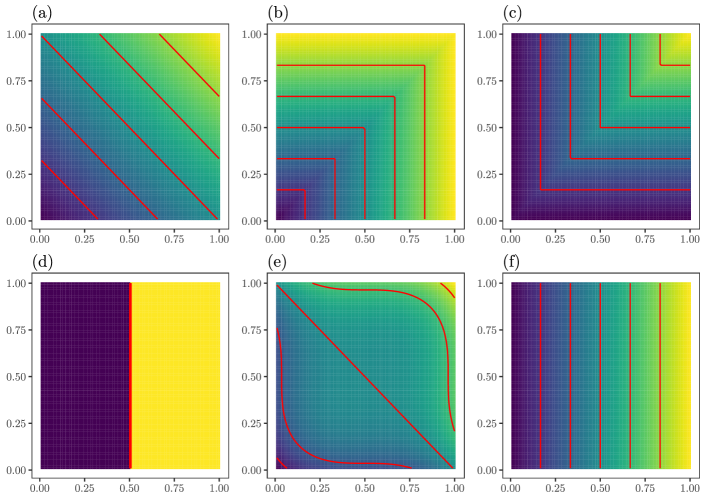
Figure 4: For $d=2$, the contour lines (red) of the regression functions corresponding to the functions $f$ in Table 1 at the levels $k/6$ for $k\in[5]$ are shown. The fill colour indicates the function value at the respective position from $0$ (purple) to $1$ (yellow).

Although we are not aware of other proposed methods for isotonic subgroup selection, there are alternative ways in which we could combine our $p$-values with different DAG testing procedures to form a data-dependent selection set. For instance, one could apply Holm’s procedure (Holm,, 1979) to ensure FWER control on the data points, and then take our data-dependent selection set to be the upper hull of the set of points in $\mathcal{D}_{X,m}$ corresponding to rejected hypotheses. This simple procedure is already a uniform improvement (in terms of the size of the selected set) on the Bonferroni approach to constructing a one-sided confidence band for $\eta$ that was mentioned in the introduction. Alternatively, one could combine our $p$-values with either the all-parent or any-parent version of the DAG testing procedure due to Meijer and Goeman, (2015), which is described in detail in Section C.1, and which we applied with uniform weights on the leaf nodes. Although we are able to prove in Section C.2 that these latter procedures have sub-optimal worst-case performance, they remain a natural approach to controlling the FWER for DAG-structured hypotheses. We refer to these three alternative versions of our procedure as $\hat{A}^{\mathrm{ISS},\mathrm{H}}$, $\hat{A}^{\mathrm{ISS},\mathrm{All}}$ and $\hat{A}^{\mathrm{ISS},\mathrm{Any}}$ respectively. In all cases, we took $m=n$, used $\tilde{p}^{1/2}$ given in Definition 18 as $p$-values and for each data-dependent selection set $\hat{A}$ we estimated $\mathbb{E}\bigl{\{}\mu\bigl{(}\mathcal{X}_{\tau}(\eta)\setminus\hat{A}\bigr{)}\bigr{\}}$ using a Monte Carlo approximation based on $10^{5}$ independent draws from $\mu$ for each data realisation, averaged over 100 repetitions of each experiment. A comparison of the running times given in Appendix B.2 shows that $\hat{A}^{\mathrm{ISS}}$ can be as much as 10 times faster to compute than $\hat{A}^{\mathrm{ISS},\mathrm{All}}$ and $\hat{A}^{\mathrm{ISS},\mathrm{Any}}$, though it is not as fast as the more naive $\hat{A}^{\mathrm{ISS},\mathrm{H}}$.

The results for regression functions (a)–(f) are presented in Figures 5, 6 and 7 respectively. Corresponding results for the other eight regression functions defined in Appendix B, which are qualitatively similar, are given in Figures 13, 14 and 15. Moreover, in Figures 16 and 17, we compare $\hat{A}^{\mathrm{ISS}}$ with two different possible approaches based on sample splitting that are of a similar flavour to the two-stage approaches mentioned in the introduction. These were omitted from our earlier comparisons for visual clarity, and because their performance turns out not to be competitive. From all of these figures, we see that $\hat{A}^{\mathrm{ISS}}$ is the most effective of these approaches for combining our $p$-values with a DAG testing procedure. The differences between $\hat{A}^{\mathrm{ISS}}$ and the other approaches are more marked when $d=2$ than in higher dimensions. It is also notable that regression functions with smaller values of $\gamma(P)$ such as (d) yield much smaller estimates of $\mathbb{E}\bigl{\{}\mu\bigl{(}\mathcal{X}_{\tau}(\eta)\setminus\hat{A}\bigr{)}\bigr{\}}$ that decay more rapidly with the sample size. Conversely, for settings with larger values of $\gamma(P)$, such as (e), the decay of our estimates of $\mathbb{E}\bigl{\{}\mu\bigl{(}\mathcal{X}_{\tau}(\eta)\setminus\hat{A}\bigr{)}\bigr{\}}$ is much slower. These observations are in agreement with our theory in Section 3.2. Finally, we remark that our procedures appear to adapt well to settings where the regression function depends only on a subset of the $d$ variables, as can be seen for instance by comparing the results in (a) and (f).

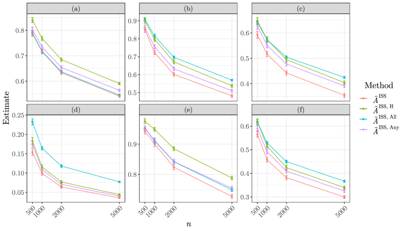
Figure 5: Estimates of $\mathbb{E}\bigl{\{}\mu\bigl{(}\mathcal{X}_{\tau}(\eta)\setminus\hat{A}\bigr{)}\bigr{\}}$ for $d=2$ and $\sigma=1/4$.

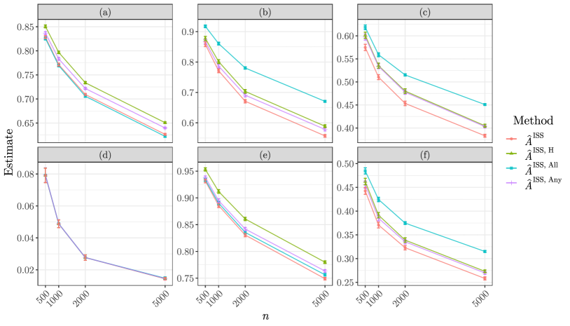
Figure 6: Estimates of $\mathbb{E}\bigl{\{}\mu\bigl{(}\mathcal{X}_{\tau}(\eta)\setminus\hat{A}\bigr{)}\bigr{\}}$ for $d=3$ and $\sigma=1/16$.

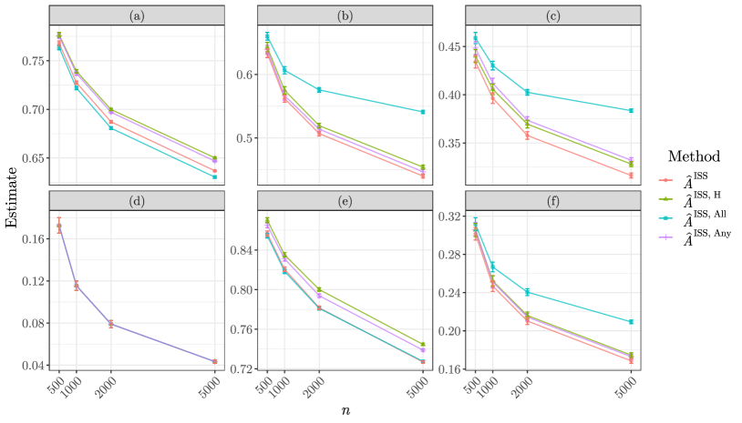
Figure 7: Estimates of $\mathbb{E}\bigl{\{}\mu\bigl{(}\mathcal{X}_{\tau}(\eta)\setminus\hat{A}\bigr{)}\bigr{\}}$ for $d=4$ and $\sigma=1/64$.

6 Real data applications

6.1 ACTG 175

As a first illustration of our procedure on real data, we consider the AIDS Clinical Trials Group Study 175 (ACTG 175) data. This was a randomised controlled trial in which HIV-1 patients whose CD4 cell counts at screening were between 200 to 500 cells per cubic millimetre and who had no history of AIDS-defining events were randomly assigned to one of four treatment groups (Hammer et al.,, 1996). We restrict our attention to two of these four treatment arms, comparing the effects of monotherapy through the antiretroviral medication zidovudine against the effects of a combination therapy of zidovudine together with zalcitabine. At the time, patient heterogeneity with respect to the response to these treatments was not well understood (Burger et al.,, 1994). Moreover, prior studies suggested that the beneficial effects of zidovudine fade with time and that this could be remedied with multitherapy (Hammer et al.,, 1996). ACTG 175 aimed to investigate treatment effect heterogeneity, in particular with respect to prior drug exposure, among patients with less advanced HIV disease. Besides relevant parts of their medical records, covariates including age, weight and ethnicity were recorded. The primary end point of the study was defined as a reduction of the CD4 cell count by at least 50%, development of AIDS, or death, with a median follow-up duration of 143 weeks (Hammer et al.,, 1996). The data for 2139 patients are freely available in the R package speff2trial (Juraska et al.,, 2022).

6.1.1 Risk group estimation

We first consider the task of identifying the patient subgroup whose probability of not reaching the primary endpoint when receiving zidovudine alone (532 patients in total) is at least $\tau=0.5$ based on their age, which the study’s eligibility criteria required to be at least $12$ years. To that end, for $i\in[n]$, let $Y_{i}=1$ if the $i$th patient did not reach the primary endpoint and $Y_{i}=0$ otherwise. Furthermore, let $X_{i}$ denote the $i$th patient’s age (multiplied by $-1$), since a decrease in age is expected to correspond to an increased probability of avoiding the primary end point across the eligible age range. Under the assumption that $\mathcal{D}=\bigl{(}(X_{1},Y_{1}),\ldots,(X_{n},Y_{n})\bigr{)}\sim P^{n}$, we then have that $P\in\mathcal{P}_{\mathrm{Mon},1}(1/2)$, so Type I error control for our procedure $\hat{A}^{\mathrm{ISS}}$ is guaranteed by Theorem 9. The left panel of Figure 8 illustrates the data-dependent selection set that we output with $\alpha=0.05$, indicating that not reaching the primary endpoint is the more likely outcome for patients aged 39 and under.

For a bivariate illustration, we use age multiplied by $-1$ and CD4 cell count at the trial onset as covariates. A high initial CD4 cell count is expected to be associated with a lower risk of reaching the primary endpoint. Thus, we assume that $\mathcal{D}\sim P^{n}$ for some $P\in\mathcal{P}_{\mathrm{Mon},2}(1/2)$, and the right panel of Figure 8 illustrates the output $\hat{A}^{\mathrm{ISS}}$ for $\tau=0.5$ and $\alpha=0.05$. The fact that the left-hand extreme of this selected set is slightly below 39 years is a reflection of the stronger form of Type I error control sought in the larger dimension.

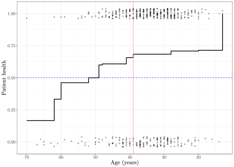
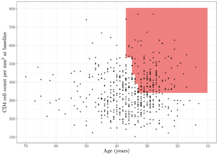
Figure 8: Left: Each black dot represents one patient in $\mathcal{D}$ (with the response jittered vertically for clarity) and the red line gives the lower bound of $\hat{A}^{\mathrm{ISS}}_{\sigma,\tau,\alpha,m}(\mathcal{D})$ when applied with the $p$-values $\tilde{p}^{1/2}$, for $\sigma=1/2$, $\tau=1/2$, $\alpha=0.05$, $m=n=532$. The black line shows the isotonic least squares regression estimator and the blue dashed line indicates the level $\tau$. Right: corresponding bivariate illustration, where the red region indicates $\hat{A}^{\mathrm{ISS}}$.

6.1.2 Heterogeneous treatment effects

To illustrate an application of the methodology of Section 4.3.1, we take the change in CD4 cell count from trial onset to week 20 ($\pm$5 weeks) as the measured response $\tilde{Y}_{i}$ for the $i$th patient. We further set $T_{i}=0$ if the $i$th patient was in the control group receiving monotherapy with zidovudine (532 patients) and $T_{i}=1$ if they were assigned to receive multitherapy with zidovudine and zalcitabine (524 patients). We are interested in identifying the subgroup for which multitherapy is at least as good as monotherapy, in the sense that the CD4 cell count is decreased by less, based on the patient’s age (again multiplied by $-1$), denoted by $X_{i}$ for the $i$th patient. This means that, conditional on treatment $T_{i}$ and age $X_{i}$, $\tilde{\eta}^{T_{i}}(X_{i})$ is the expected change in CD4 cell count in the first 20 weeks, and we assume that the observed response $\tilde{Y}_{i}$ is conditionally symmetrically distributed around $\tilde{\eta}^{T_{i}}(X_{i})$. Thus $\eta(x):=\tilde{\eta}^{1}(x)-\tilde{\eta}^{0}(x)$ gives the heterogeneous treatment effect on the change in CD4 cell count for patients of $x$ years of age, and we are interested in identifying $\mathcal{X}_{0}(\eta)$ under the assumption that this is an upper set. Here, $\pi(x)=1/2$ for all $x$, so that from (4), $Y_{i}=(4T_{i}-2)\cdot\tilde{Y}_{i}$ for all $i$. Defining now $Y^{*}_{i}:=\mathbbm{1}_{\{Y_{i}\geq 0\}}$ and assuming $\mathcal{D}^{0}=\bigl{(}(X_{1},Y^{*}_{1}),\ldots,(X_{n},Y^{*}_{n})\bigr{)}\sim P^{n}$, we have $P\in\mathcal{P}_{\mathrm{Upp},1}(1/2,1/2)$, so that $\hat{A}^{\mathrm{ISS}}$ when applied with $\check{p}_{1/2}$ controls the Type I error by the discussion in Section 4.3.1. See Figure 9 for a visualisation of the result. We conclude that among patients aged 25 or younger, replacing monotherapy by multitherapy is uniformly associated with a neutral or beneficial effect on the stability of CD4 cell count.

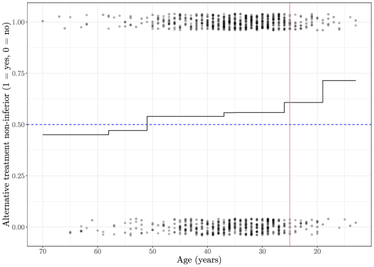
Figure 9: Each black dot represents one patient in $\mathcal{D}$ (with $Y_{i}^{*}$ jittered vertically for clarity) and the red line gives the lower bound of $\hat{A}^{\mathrm{ISS}}_{\sigma,\tau,\alpha,m}(\mathcal{D})$ when applied with $\check{p}_{\tau}$, $\tau=1/2$, $\alpha=0.05$, $m=n=1056$. Further, the black line shows the isotonic least squares regression estimator. The blue dashed line indicates the level $\tau$.

6.2 Fuel consumption dataset

Here we consider the Auto MPG dataset that was popularised by Quinlan, (1993) and that is available through the UCI Machine Learning Repository (Dua and Graff,, 2019). This dataset contains information on $n=398$ cars, including their urban fuel consumption, weight and engine displacement. We would like to identify the combinations of car weight and engine displacement for which the probability of fuel efficiency being at least 15mpg is at least $\tau=0.5$. To this end, we set $Y_{i}=1$ if the $i$th car’s fuel efficiency is at least 15mpg and $Y_{i}=0$ otherwise. Since increases in weight and engine displacement can be assumed to decrease the conditional probability of high fuel efficiency, we let the two components of $X_{i}\in(-\infty,0)^{2}$ give the $i$th car’s weight and engine displacement (multiplied by $-1$). We then have that $\mathcal{D}=\bigl{(}(X_{1},Y_{1}),\ldots(X_{n},Y_{n})\bigr{)}\sim P^{n}$ with $P\in\mathcal{P}_{\mathrm{Mon,2}}(1/2)$, so Type I error control for our procedure $\hat{A}^{\mathrm{ISS}}$ is guaranteed by Theorem 9. The output set from the $\hat{A}^{\mathrm{ISS}}$ algorithm is shown in Figure 10. The strong sample correlation of 0.93 between weight and engine displacement contributes to the data-dependent selection set being almost rectangular, with a weight of under 3400lbs and an engine displacement of under 250 cubic inches being sufficient to be fairly confident that the fuel consumption is more likely than not to be at least 15mpg.

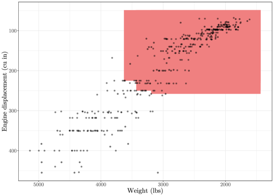
Figure 10: Each black dot represents one car in $\mathcal{D}_{X}$ and the red area gives the output of $\hat{A}^{\mathrm{ISS}}_{\sigma,\tau,\alpha,m}(\mathcal{D})$ applied with $\tilde{p}_{\sigma,\tau}^{1/2}$ for $\sigma=1/2$, $\tau=1/2$, $\alpha=0.05$, $m=n=398$.

Appendix

Section A of this appendix consists of proofs of all of our main results, as well as statements and proofs of intermediate results. Section B presents further simulations, while Section C contains a discussion of an alternative and general approach to combining the $p$-values due to Meijer and Goeman, (2015). Finally, in Section D, we give a few auxiliary results.

Appendix A Proofs

We begin with some additional notation used in the appendix. For a set $A\subseteq\mathbb{R}^{d}$, let $\mathrm{Pow}(A)$ denote the power set of $A$. Denote by $\|\cdot\|_{2}$ the Euclidean norm on $\mathbb{R}^{d}$ and for $x\in\mathbb{R}^{d}$ and $r>0$, define the closed Euclidean norm ball by ${B}_{2}(x,r):=\{z\in\mathbb{R}^{d}:\|z-x\|_{2}\leq r\}$. Given $A_{0}$, $A_{1}\subseteq\mathbb{R}^{d}$, we write $A_{0}\preccurlyeq A_{1}$ if $x_{0}\preccurlyeq x_{1}$ for every pair $(x_{0},x_{1})\in A_{0}\times A_{1}$. We write $\mathcal{L}_{d}$ for Lebesgue measure on $\mathbb{R}^{d}$. Finally, for $r\geq 0$ and $x\in\mathbb{R}^{d}$, we denote $\mathcal{I}_{r}(x)\equiv\mathcal{I}_{r}(x,\mathcal{D}_{X}):=\{i\in[n]:X_{i}\preccurlyeq x,\|X_{i}-x\|_{\infty}\leq r\}$.

A.1 Proofs from Section 3.1

In order to verify Lemma 5 it will be convenient to prove the following small generalisation.

Lemma 25.

Let $\sigma>0$, $\tau\in\mathbb{R}$ and let $P$ be a distribution on $\mathbb{R}^{d}\times\mathbb{R}$ with regression function $\eta$ such that if $(X,Y)\sim P$, then $Y-\eta(X)$ is conditionally sub-Gaussian with variance parameter $\sigma^{2}$ given $X$. Fix $x\in\mathbb{R}^{d}$ and suppose that $\eta(x^{\prime})\leq\tau$ for all $x^{\prime}\preccurlyeq x$. Given $\mathcal{D}=\bigl{(}(X_{1},Y_{1}),\ldots,(X_{n},Y_{n})\bigr{)}\sim P^{n}$, we have $\mathbb{P}_{P}\bigl{\{}\hat{p}_{\sigma,\tau}(x,\mathcal{D})\leq\alpha|\mathcal{D}_{X}\bigr{\}}\leq\alpha$ for all $\alpha\in(0,1)$.

Proof of Lemma 25 (and hence Lemma 5).

Throughout the proof, we operate conditional on $\mathcal{D}_{X}$ and consider the setting of Definition 1. If $\mathcal{I}(x)=\emptyset$, then $\hat{p}_{\sigma,\tau}(x,\mathcal{D})=1$ and the result follows, so suppose henceforth that $n(x)\geq 1$. Define the $\sigma$-algebra $\mathcal{F}_{0}$ generated by $\{(X_{i})_{i\in\mathcal{I}(x)}\}$ and the $\sigma$-algebras $\mathcal{F}_{k}$ generated by $\bigl{\{}\bigl{(}Y_{(j)}(x)\bigr{)}_{j\in[k]}\cup\mathcal{F}_{0}\bigr{\}}$ for $k\in[n(x)]$. Similarly to the proof of Duan et al., (2020, Theorem 3), we first show that $(S_{k})_{k\in\{0\}\cup[n(x)]}$,where $S_{0}:=0$, is a supermartingale with respect to the filtration $(\mathcal{F}_{k})_{k\in\{0\}\cup[n(x)]}$. Since for $k\in[n(x)]$, $S_{k-1}$ is measurable with respect to $\mathcal{F}_{k-1}$ and the ordering $Y_{(1)},\ldots,Y_{(n(x))}$ is fixed conditional on $\mathcal{D}_{X}$, we have for any $k\in[n(x)]$ that

$$\mathbb{E}(S_{k}\mid\mathcal{F}_{k-1}) =S_{k-1}+\frac{1}{\sigma}\bigl{\{}\mathbb{E}\bigl{(}Y_{(k)}(x)\mid\mathcal{F}_{k-1}\bigr{)}-\tau\bigr{\}}$$

$$=S_{k-1}+\frac{1}{\sigma}\bigl{\{}\eta\bigl{(}X_{(k)}(x)\bigr{)}-\tau\bigr{\}}\leq S_{k-1},$$

where in the last step we used the fact that $\eta(X_{i})\leq\eta(x)\leq\tau$ for $i\in\mathcal{I}(x)$. Since the integrability of $S_{k}$ follows from the sub-Gaussianity of the increments, the sequence $(S_{k})_{k\in\{0\}\cup[n(x)]}$ is a supermartingale. Moreover, its increments satisfy $Z^{\prime}_{k}:=S_{k}-S_{k-1}=\bigl{(}Y_{(k)}(x)-\tau\bigr{)}/\sigma\leq\bigl{\{}Y_{(k)}(x)-\eta\bigl{(}X_{(k)}(x)\bigr{)}\bigr{\}}/\sigma=:Z_{k}$ for $k\in[n(x)]$ and the random variables $(Z^{\prime}_{k})_{k\in[n(x)]}$ are independent conditional on $\mathcal{D}_{X}$, as are $(Z_{k})_{k\in[n(x)]}$. Thus, we have by Lemma 45(a) and with $u_{\alpha}(\cdot)$ as defined there that

$$\mathbb{P}\biggl{(}\bigcup_{k=1}^{n(x)}\bigl{\{}S_{k}\geq u_{\alpha}(k)\}\,\biggm{|}\,\mathcal{D}_{X}\biggr{)} =\mathbb{P}\biggl{(}\bigcup_{k=1}^{n(x)}\biggl{\{}\sum_{j=1}^{k}Z^{\prime}_{j}\geq u_{\alpha}(k)\biggr{\}}\,\biggm{|}\,\mathcal{D}_{X}\biggr{)}$$

$$\leq\mathbb{P}\biggl{(}\bigcup_{k=1}^{n(x)}\biggl{\{}\sum_{j=1}^{k}Z_{j}\geq u_{\alpha}(k)\biggr{\}}\,\biggm{|}\,\mathcal{D}_{X}\biggr{)}\leq\alpha.$$

Hence, for $\alpha\in(0,1)$,

$$\mathbb{P}\bigl{(}\hat{p}_{\sigma,\tau}(x,\mathcal{D})\leq\alpha\mid\mathcal{D}_{X}\bigr{)} =\mathbb{P}\bigl{(}\hat{p}_{\sigma,\tau}(x,\mathcal{D})\leq\alpha,n(x)>0\mid\mathcal{D}_{X}\bigr{)}$$

$$=\mathbb{P}\biggl{(}\max_{k\in[n(x)]}\frac{S_{k}}{u_{\alpha}(k)}\geq 1,n(x)>0\Bigm{|}\mathcal{D}_{X}\biggr{)}\leq\alpha,$$

as required. ∎

Proof of Lemma 8.

Fix a finite set $I$, a family of distributions $\mathcal{Q}$ on $(0,1]^{I}$, a collection of random variables $\bm{p}=(p_{i})_{i\in I}$ taking values in $(0,1]^{I}$, as well as hypotheses $H_{i}\subseteq\{Q\in\mathcal{Q}:\mathbb{P}_{Q}(p_{i}\leq t)\leq t,\forall t\in(0,1]\}$ for $i\in I$ and any $G_{0}$-consistent polyforest-weighted DAG $G^{\prime}=(I,E,\bm{w})$. Throughout this proof, define $G:=(I,E)$ and $F:=(I,\{e\in E:w_{e}=1\})$ as in Algorithm 1, and write $J^{c}:=I\setminus J$ for any $J\subseteq I$. Fix $Q_{0}\in\mathcal{Q}$, so that $I_{0}\equiv I_{0}(Q_{0})\subseteq I$ is a $G$-lower set giving the indices of true null hypotheses. If $I_{0}=\emptyset$, then no Type I error can be made and the proof is complete. We therefore suppose henceforth that $|I_{0}|>0$. For a proper subset $J$ of $I$, it is convenient to define

$$\alpha(i,J)\equiv\alpha(i,J,F):=\begin{cases}\frac{|(\{i\}\cup\operatorname{\mathrm{de}}_{F}(i))\cap L(F)\cap J^{c}|}{|L(F)\cap J^{c}|}\cdot\alpha\quad&\text{if $i\notin J$, $\operatorname{\mathrm{pa}}_{F}(i)\subseteq J$}\\ 0&\text{otherwise.}\end{cases}$$ (5)

Thus, given a set of rejected hypotheses $J$ at a particular iteration of Algorithm 1 and writing $\mathcal{N}_{0}(J):=\{i\in J^{c}:p_{i}\leq\alpha(i,J)\}$, the hypotheses in $\mathcal{N}(J):=\mathcal{N}_{0}(J)\cup\bigcup_{j\in\mathcal{N}_{0}(J)}\operatorname{\mathrm{an}}_{G}(j)$ will be rejected at the next iteration. Hence, the set of rejected hypotheses at the $\ell$-th iteration in Algorithm 1 can be written as $R_{\ell}=R_{\ell-1}\cup\mathcal{N}(R_{\ell-1})$ with $R_{0}=\emptyset$. We first claim that

$$\mathcal{N}(I_{1})\subseteq\mathcal{N}(I_{2})\cup I_{2}$$ (6)

for all $G$-upper proper subsets $I_{1}\subseteq I_{2}$ of $I$. To see this, fix such $I_{1},I_{2}$ and any $i\in\mathcal{N}(I_{1})$. The result is immediate if $i\in I_{2}$, so suppose that $i\in I_{2}^{c}$. If $i\in\mathcal{N}_{0}(I_{1})$, then $\alpha(i,I_{1})>0$, so $\operatorname{\mathrm{pa}}_{F}(i)\subseteq I_{1}$. Since $I_{1}$ and $I_{2}$ are $G$-upper, they are also $F$-upper. Hence $\{i\}\cup\operatorname{\mathrm{de}}_{F}(i)\subseteq I^{c}_{2}\subseteq I^{c}_{1}$, so that

$$\alpha(i,I_{1})=\frac{\bigl{|}\bigl{(}\{i\}\cup\operatorname{\mathrm{de}}_{F}(i)\bigr{)}\cap L(F)\bigr{|}}{|L(F)\cap I_{1}^{c}|}\cdot\alpha\leq\frac{\bigl{|}\bigl{(}\{i\}\cup\operatorname{\mathrm{de}}_{F}(i)\bigr{)}\cap L(F)\bigr{|}}{|L(F)\cap I_{2}^{c}|}\cdot\alpha=\alpha(i,I_{2}),$$ (7)

and we deduce that $i\in\mathcal{N}_{0}(I_{2})\subseteq\mathcal{N}(I_{2})$. If instead $i\in\operatorname{\mathrm{an}}_{G}(j_{0})$ for some $j_{0}\in\mathcal{N}_{0}(I_{1})$, then since $I_{2}$ is $G$-upper and $i\in I_{2}^{c}$, we have $j_{0}\in I_{2}^{c}$. Following the same line of reasoning as in (7), we see that $0<\alpha(j_{0},I_{1})\leq\alpha(j_{0},I_{2})$, so that $j_{0}\in\mathcal{N}_{0}(I_{2})$ and consequently $i\in\operatorname{\mathrm{an}}_{G}(j_{0})\subseteq\mathcal{N}(I_{2})$. This establishes the claim in (6).

Our second claim is that

$$\mathbb{P}_{Q_{0}}\bigl{(}\mathcal{N}(I^{c}_{0})=\emptyset\bigr{)}\geq 1-\alpha.$$ (8)

To see this, first note that since $I_{0}^{c}$ is $G$-upper, it is $F$-upper. Moreover, for any $i\in I_{0}$, we have $\alpha(i,I_{0}^{c})>0$ only if $\operatorname{\mathrm{pa}}_{F}(i)\subseteq I_{0}^{c}$, so the ancestors of any element of $I_{*}:=\{i\in I_{0}:\alpha(i,I_{0}^{c})>0\}$ belong to $I_{0}^{c}$, and we deduce that $I_{*}$ is an antichain in $F$. Combining this with the fact that $F$ is a polyforest in which each node has at most one parent, we see that if $i_{1},i_{2}\in I_{*}$ are distinct, then $\{i_{1}\}\cup\operatorname{\mathrm{de}}_{F}(i_{1})$ and $\{i_{2}\}\cup\operatorname{\mathrm{de}}_{F}(i_{2})$ are disjoint. Hence,

$$\mathbb{P}_{Q_{0}}\bigl{(}\mathcal{N}(I^{c}_{0})\neq\emptyset\bigr{)} =\mathbb{P}_{Q_{0}}\biggl{(}\bigcup_{i\in I_{0}}\bigl{\{}p_{i}\leq\alpha(i,I_{0}^{c})\bigr{\}}\biggr{)}\leq\sum_{i\in I_{0}}\mathbb{P}_{Q_{0}}\bigl{(}p_{i}\leq\alpha(i,I_{0}^{c})\bigr{)}$$

$$\leq\sum_{i\in I_{0}}\alpha(i,I_{0}^{c})=\sum_{i\in I_{*}}\frac{\bigl{|}\bigl{(}\{i\}\cup\operatorname{\mathrm{de}}_{F}(i)\bigr{)}\cap L(F)\bigr{|}}{|L(F)\cap I_{0}|}\cdot\alpha\leq\alpha,$$

as required. Writing $\Omega_{0}:=\bigl{\{}\mathcal{N}(I_{0}^{c})\cap I_{0}=\emptyset\bigr{\}}$ and using (6), we see that $\mathcal{N}(R_{\ell-1})\subseteq\mathcal{N}(I_{0}^{c})\cup I_{0}^{c}$, so on $\Omega_{0}$, we have $\mathcal{N}(R_{\ell-1})\subseteq I_{0}^{c}$. We deduce that

$$\Omega_{0}\cap\{R_{\ell-1}\cap I_{0}=\emptyset\}=\Omega_{0}\cap\{\mathcal{N}(R_{\ell-1})\cap I_{0}=\emptyset\}\cap\{R_{\ell-1}\cap I_{0}=\emptyset\}=\Omega_{0}\cap\{R_{\ell}\cap I_{0}=\emptyset\}.$$

Since $R_{0}=\emptyset$, we have $\Omega_{0}=\Omega_{0}\cap\{R_{0}\cap I_{0}=\emptyset\}$, which yields by induction that $\Omega_{0}=\Omega_{0}\cap\{R_{|I|}\cap I_{0}=\emptyset\}\subseteq\{R_{|I|}\cap I_{0}=\emptyset\}$. Combining this with (8) we conclude that

$$\mathbb{P}_{Q_{0}}\bigl{(}R_{|I|}\cap I_{0}=\emptyset\bigr{)}\geq\mathbb{P}_{Q_{0}}(\Omega_{0})=\mathbb{P}_{Q_{0}}\bigl{(}\mathcal{N}(I_{0}^{c})=\emptyset\bigr{)}\geq 1-\alpha,$$

as required. ∎

Proof of Theorem 9.

If $(\mathcal{X},\mathcal{A})$ and $(\mathcal{Y},\mathcal{B})$ are measurable spaces, $f:\mathcal{X}\rightarrow\mathcal{Y}$ is measurable and $\pi$ is a distribution on $\mathcal{X}$, let $f\sharp\pi$ denote the pushforward measure on $\mathcal{Y}$ of $\pi$ under $f$; i.e., if $Z\sim\pi$ then $f(Z)\sim f\sharp\pi$. We condition on $\mathcal{D}_{X}$ throughout this proof and denote $\hat{\bm{p}}^{*}\equiv\hat{\bm{p}}^{*}(\cdot)=\bigl{(}\hat{p}_{i}^{*}(\cdot)\bigr{)}_{i\in[m]}:=\bigl{(}\hat{p}_{\sigma,\tau}(X_{i},\cdot)\bigr{)}_{i\in[m]}$. Write $\mathcal{Q}:=\{\hat{\bm{p}}^{*}\sharp\tilde{P}^{n}:\tilde{P}\in\mathcal{P}_{\mathrm{Mon},d}(\sigma)\}$ for a family of distributions over $(0,1]^{m}$ induced by $\mathcal{P}_{\mathrm{Mon},d}(\sigma)$. Further, for $i\in[m]$, let $H^{*}_{i}:=\{\tilde{P}\in\mathcal{P}_{\mathrm{Mon},d}(\sigma):\mathbb{E}_{\tilde{P}}(Y_{i}|X_{i})<\tau\}$ and $H_{i}:=\{\hat{\bm{p}}^{*}\sharp\tilde{P}^{n}:\tilde{P}\in H_{i}^{*}\}\subseteq\mathcal{Q}$, so that for $Q:=\hat{\bm{p}}^{*}\sharp P^{n}$ we have $I_{0}(P):=\{i\in[m]:P\in H^{*}_{i}\}\subseteq\{i\in[m]:Q\in H_{i}\}=:I_{0}(Q)$. Lemma 5 then shows that $H_{i}\subseteq\{\tilde{Q}\in\mathcal{Q}:\mathbb{P}_{\tilde{Q}}(\hat{p}^{*}_{i}\leq t|\mathcal{D}_{X})\leq t\ \forall t\in(0,1]\}$. Now define $G_{0}^{*}:=([m],E_{0}^{*})$, where $E_{0}^{*}:=\{(i_{0},i_{1})\in[m]^{2}:H_{i_{0}}^{*}\subseteq H_{i_{1}}^{*}\}$ and $G_{0}:=([m],E_{0})$, where $E_{0}:=\{(i_{0},i_{1})\in[m]^{2}:H_{i_{0}}\subseteq H_{i_{1}}\}$. We claim that $E_{0}^{*}\subseteq E_{0}$. To see this, fix $(i_{0},i_{1})\in E_{0}^{*}$, so that $H_{i_{0}}^{*}\subseteq H_{i_{1}}^{*}$, and suppose that $Q_{0}\in H_{i_{0}}$. Then we can find $P_{0}\in H_{i_{0}}^{*}$ such that $Q_{0}=\hat{\bm{p}}^{*}\sharp P_{0}^{n}$. But since $P_{0}\in H_{i_{1}}^{*}$, we must have that $Q_{0}\in H_{i_{1}}$, and this establishes our claim. By construction, $\mathcal{G}_{\mathrm{W}}(\mathcal{D}_{X,m})$ is a $G_{0}^{*}$-consistent polyforest-weighted DAG, and we can therefore deduce from our claim that it is also a $G_{0}$-consistent polyforest-weighted DAG. Hence, by Lemma 8,

$$\mathbb{P}_{P}\bigl{\{}\mathcal{R}_{\alpha}^{\mathrm{ISS}}\bigl{(}\mathcal{G}_{\mathrm{W}}(\mathcal{D}_{X,m}), \hat{\bm{p}}^{*}(\mathcal{D})\bigr{)}\cap I_{0}(P)=\emptyset\bigm{|}\mathcal{D}_{X}\bigr{\}}$$

$$\geq\mathbb{P}_{Q}\bigl{\{}\mathcal{R}_{\alpha}^{\mathrm{ISS}}\bigl{(}\mathcal{G}_{\mathrm{W}}(\mathcal{D}_{X,m}),\hat{\bm{p}}^{*}\bigr{)}\cap I_{0}(Q)=\emptyset\bigm{|}\mathcal{D}_{X}\bigr{\}}\geq 1-\alpha.$$

Moreover, $\mathcal{X}_{\tau}(\eta)$ is an upper set because $P\in\mathcal{P}_{\mathrm{Mon},d}(\sigma)$, and we conclude that

$$\mathbb{P}_{P}\bigl{(}\hat{A}^{\mathrm{ISS}}_{\sigma,\tau,\alpha,m}(\mathcal{D})\subseteq\mathcal{X}_{\tau}(\eta)\bigm{|}\mathcal{D}_{X}\bigr{)}\geq\mathbb{P}_{P}\bigl{\{}\mathcal{R}_{\alpha}^{\mathrm{ISS}}\bigl{(}\mathcal{G}_{\mathrm{W}}(\mathcal{D}_{X,m}),\hat{\bm{p}}^{*}(\mathcal{D})\bigr{)}\cap I_{0}(P)=\emptyset\bigm{|}\mathcal{D}_{X}\bigr{\}}\geq 1-\alpha,$$

as required. ∎

A.2 Proofs from Section 3.2

The following proposition shows that if we only know that $P\in\mathcal{P}_{\mathrm{Mon},d}(\sigma)$, then it is impossible to provide non-trivial uniform power guarantees for data-dependent selection sets with Type I error control.

Proposition 26.

Let $d\in\mathbb{N}$, $\tau\in\mathbb{R}$, $\sigma>0$ and $\alpha\in(0,1)$. Then, for any $n\in\mathbb{N}$,

$$\sup_{P\in\mathcal{P}_{\mathrm{Mon},d}(\sigma)}\inf_{\hat{A}\in\hat{\mathcal{A}}_{n}(\tau,\alpha,\mathcal{P}_{\mathrm{Mon},d}(\sigma))}\mathbb{E}_{P}\bigl{\{}\mu\bigl{(}\mathcal{X}_{\tau}(\eta)\setminus\hat{A}(\mathcal{D})\bigr{)}\bigr{\}}\geq 1-\alpha.$$

Proof of Proposition 26.

Fix a Borel probability measure $\mu$ on $\mathbb{R}^{d}$. For $\Delta\in\mathbb{R}$, let $\eta_{\Delta}:\mathbb{R}^{d}\rightarrow\mathbb{R}$ denote the constant function satisfying $\eta_{\Delta}(x):=\tau+\Delta$ for all $x\in\mathbb{R}^{d}$, and let $P_{\Delta}$ denote the distribution on $\mathbb{R}^{d}\times\mathbb{R}$ of $(X,Y)$, where $X\sim\mu$ and $Y|X\sim\mathcal{N}\bigl{(}\eta_{\Delta}(X),\sigma^{2}\bigr{)}$. Thus $\{P_{\Delta}:\Delta\in\mathbb{R}\}\subseteq\mathcal{P}_{\mathrm{Mon},d}(\sigma)$. Moreover, for any $\Delta>0$, we have by Pinsker’s inequality that

$$\mathrm{TV}(P_{-\Delta}^{n},P_{0}^{n}) \leq\sqrt{\frac{n}{2}\cdot\mathrm{KL}(P_{-\Delta},P_{0})}=\sqrt{\frac{n}{2}\cdot\mathrm{KL}\bigr{(}\mathcal{N}(\tau-\Delta,\sigma^{2}),\mathcal{N}(\tau,\sigma^{2})\bigr{)}}\leq\frac{\sqrt{n}\Delta}{2\sigma}.$$

Now fix $\Delta>0$, and suppose that $\hat{A}\in\hat{\mathcal{A}}_{n}\bigl{(}\tau,\alpha,\mathcal{P}_{\mathrm{Mon},d}(\sigma)\bigr{)}$. Since $\mathcal{X}_{\tau}(\eta_{-\Delta})=\emptyset$, we have for every $x\in\mathbb{R}^{d}$ that

$$\mathbb{P}_{P_{0}}\bigl{(}x\in\hat{A}(\mathcal{D})\bigr{)} \leq\mathbb{P}_{P_{-\Delta}}\bigl{(}x\in\hat{A}(\mathcal{D})\bigr{)}+\mathrm{TV}\bigl{(}P_{-\Delta}^{n},P_{0}^{n}\bigr{)}$$

$$\leq\mathbb{P}_{P_{-\Delta}}\bigl{(}\hat{A}(\mathcal{D})\nsubseteq\mathcal{X}_{\tau}(\eta_{-\Delta})\bigr{)}+\frac{\sqrt{n}\Delta}{2\sigma}\leq\alpha+\frac{\sqrt{n}\Delta}{2\sigma}.$$

Hence, by Fubini’s theorem,

$$\mathbb{E}_{P_{0}}\bigl{\{}\mu\bigl{(}\hat{A}(\mathcal{D})\bigr{)}\bigr{\}}=\mathbb{E}_{P_{0}}\biggl{(}\int_{\mathbb{R}^{d}}\mathbbm{1}_{\{x\in\hat{A}(\mathcal{D})\}}\,d\mu(x)\biggr{)}=\int_{\mathbb{R}^{d}}\mathbb{P}_{P_{0}}\bigl{(}x\in\hat{A}(\mathcal{D})\bigr{)}\,d\mu(x)\leq\alpha+\frac{\sqrt{n}\Delta}{2\sigma}.$$

Moreover, by our choice of $\eta_{0}$, we have $\mathcal{X}_{\tau}(\eta_{0})=\mathbb{R}^{d}$, and hence

$$\mathbb{E}_{P_{0}}\bigl{\{}\mu\bigl{(}\mathcal{X}_{\tau}(\eta_{0})\setminus\hat{A}(\mathcal{D})\bigr{)}\bigr{\}} =1-\mathbb{E}_{P_{0}}\bigl{\{}\mu\bigl{(}\hat{A}(\mathcal{D})\bigr{)}\bigr{\}}\geq 1-\alpha-\frac{\sqrt{n}\Delta}{2\sigma}.$$

The result follows by taking an infimum over $\hat{A}\in\hat{\mathcal{A}}_{n}\bigl{(}\tau,\alpha,\mathcal{P}_{\mathrm{Mon},d}(\sigma)\bigr{)}$, and then letting $\Delta\rightarrow 0$. ∎

Proof of Theorem 11.

Let us define $C_{0}:=962\geq 2\{16\vee 481^{1/(2\beta+1)}\}$ and $C:=3C_{0}$. Further, let

$$\xi:=\frac{C_{0}}{2}\biggl{\{}\biggl{(}\frac{\sigma^{2}}{n\nu^{2}}\log_{+}\Bigl{(}\frac{\log_{+}n}{\alpha\wedge\delta}\Bigr{)}\biggr{)}^{1/(2\beta+1)}+\frac{\log_{+}(1/\delta)}{n}\biggr{\}}.$$

By the choice of $\xi$, the result holds if $\mu\bigl{(}\mathcal{X}_{\tau}(\eta)\bigr{)}\leq 2\xi$. We therefore suppose henceforth that $\xi$ is such that $\xi<1/2$ and $\mu\bigl{(}\mathcal{X}_{\tau}(\eta)\bigr{)}>2\xi$. Then, since $P\in\mathcal{P}_{\mathrm{Mar},d}(\tau,\beta,\nu)$, we have that $\mu\bigl{(}\mathcal{X}_{\tau+\nu\xi^{\beta}}(\eta)\bigr{)}>\xi$, so $x_{0}:=\inf\{x\in\mathcal{X}_{\tau+\nu\xi^{\beta}}(\eta):\mu\bigl{(}\mathcal{X}_{\tau+\nu\xi^{\beta}}(\eta)\cap(-\infty,x]\bigr{)}\geq\xi\}$ is finite. For $I_{\xi}:=\mathcal{X}_{\tau+\nu\xi^{\beta}}(\eta)\cap(-\infty,x_{0}]$, it then holds that $\mu(I_{\xi})\geq\xi$. Further, by Lemma 49(i) and the fact that $C_{0}\geq 32$,

$$n\xi\geq 16\log_{+}\Bigl{(}\frac{1}{\delta}\Bigr{)}\geq 8\log\Bigl{(}\frac{2}{\delta}\Bigr{)}.$$

Writing $\Omega_{0}:=\bigl{\{}n^{-1}\sum_{i=1}^{n}\mathbbm{1}_{\{X_{i}\in I_{\xi}\}}\geq\xi/2\bigr{\}}$, it follows by a multiplicative Chernoff bound (McDiarmid,, 1998, Theorem 2.3(c)) that

$$\mathbb{P}_{P}\bigl{(}\Omega_{0}^{c}\bigr{)}\leq e^{-n\xi/8}\leq\frac{\delta}{2}.$$

By the choice of $\xi$, it holds on $\Omega_{0}$ that

$$\sum_{i=1}^{n}\mathbbm{1}_{\{X_{i}\in I_{\xi}\}}\geq\frac{n\xi}{2}\geq\frac{1}{2}\cdot\Bigl{(}\frac{C_{0}}{2}\Bigr{)}^{2\beta+1}\cdot\frac{\sigma^{2}}{\nu^{2}\xi^{2\beta}}\log_{+}\Bigl{(}\frac{\log_{+}n}{\alpha\wedge\delta}\Bigr{)};$$

in particular, since $n\xi\geq 8\log(2/\delta)$, it holds on this event that $\sum_{i=1}^{n}\mathbbm{1}_{\{X_{i}\in I_{\xi}\}}\geq 1$. Thus, we can fix any $i_{1}\in[n]$ such that $X_{i_{1}}=\max(\mathcal{D}_{X}\cap I_{\xi})$. Furthermore, let $i_{1},\ldots,i_{K}\in[n]$ with $K:=|\{i\in[n]:X_{i}\geq X_{i_{1}}\}|$ be the maximal set of indices such that $X_{i_{k}}\geq X_{i_{1}}$ for all $k\in[K]$. Writing $r_{k}:=X_{i_{k}}-\min(\mathcal{D}_{X}\cap I_{\xi})$ and noting that $\mathcal{I}_{r}(x)=\{i\in[n]:x-r\leq X_{i}\leq x\}$ for $r\geq 0$ and $x\in\mathbb{R}$, we have on $\Omega_{0}$ that for all $k\in[K]$,

$$n\geq|\mathcal{I}_{r_{k}}(X_{i_{k}})|\geq|\mathcal{I}_{r_{1}}(X_{i_{1}})|\geq\frac{1}{2}\cdot\Bigl{(}\frac{C_{0}}{2}\Bigr{)}^{2\beta+1}\cdot\frac{\sigma^{2}}{\nu^{2}\xi^{2\beta}}\log_{+}\Bigl{(}\frac{\log_{+}n}{\alpha\wedge\delta}\Bigr{)}.$$

Hence, writing $u_{\delta^{\prime}}(\ell):=1.7\sqrt{\ell\bigl{\{}0.72\log(5.2/\delta^{\prime})+\log\log(2\ell)\bigr{\}}}$ for $\delta^{\prime}\in(0,1)$ and $\ell\in\mathbb{N}$ as in Lemma 45(a), we have for all $k\in[K]$ that

$$\biggl{(}\frac{u_{\alpha}(|\mathcal{I}_{r_{k}}(X_{i_{k}})|)+u_{\delta/2}(|\mathcal{I}_{r_{k}}(X_{i_{k}})|)}{|\mathcal{I}_{r_{k}}(X_{i_{k}})|}\biggr{)}^{2}$$

$$\leq\frac{2\cdot 1.7^{2}\cdot 0.72\cdot\bigl{\{}\log(5.2/\alpha)+\log(10.4/\delta)\bigr{\}}+2\cdot 2\cdot 1.7^{2}\cdot\log\log\bigl{(}2\cdot|\mathcal{I}_{r_{k}}(X_{i_{k}})|\bigr{)}}{|\mathcal{I}_{r_{k}}(X_{i_{k}})|}$$

$$\leq\frac{2\cdot 1.7^{2}\cdot 0.72\cdot 2\cdot\log\bigl{(}\frac{10.4}{\alpha\wedge\delta}\bigr{)}+4\cdot 1.7^{2}\cdot\log\bigl{\{}2\log_{+}\bigl{(}|\mathcal{I}_{r_{k}}(X_{i_{k}})|\bigr{)}\bigr{\}}}{|\mathcal{I}_{r_{k}}(X_{i_{k}})|}$$

$$\leq 11.56\cdot\frac{\log\bigl{(}\frac{20.8\log_{+}n}{\alpha\wedge\delta}\bigr{)}}{|\mathcal{I}_{r_{1}}(X_{i_{1}})|}\leq 11.56\cdot 20.8\cdot\frac{\log_{+}\bigl{(}\frac{\log_{+}n}{\alpha\wedge\delta}\bigr{)}}{|\mathcal{I}_{r_{1}}(X_{i_{1}})|}$$

$$\leq 481\cdot\Bigl{(}\frac{2}{C_{0}}\Bigr{)}^{2\beta+1}\cdot\frac{\nu^{2}\xi^{2\beta}}{\sigma^{2}}\leq\frac{\nu^{2}\xi^{2\beta}}{\sigma^{2}},$$

where we used the inequality $(a+b)^{2}\leq 2(a^{2}+b^{2})$ for $a,b\geq 0$, Lemma 49(i) and the fact that $C_{0}\geq 2\cdot 481^{1/(2\beta+1)}$. For

$$\Omega_{1}\bigl{(}X_{i_{1}}\bigr{)}:=\bigcap_{k=1}^{K}\biggl{\{}\sum_{i\in\mathcal{I}_{r_{k}}(X_{i_{k}})}\frac{Y_{i}-\tau}{\sigma}\geq u_{\alpha}\bigl{(}|\mathcal{I}_{r_{k}}(X_{i_{k}})|\bigr{)}\biggr{\}},$$

we therefore have on $\Omega_{0}$ that

$$\mathbb{P}_{P}\Bigl{(}\Omega_{1}\bigl{(}X_{i_{1}}\bigr{)}^{c} \bigm{|}\mathcal{D}_{X}\Bigr{)}$$

$$=\mathbb{P}_{P}\biggl{(}\bigcup_{k=1}^{K}\biggl{\{}\sum_{i\in\mathcal{I}_{r_{k}}(X_{i_{k}})}\frac{Y_{i}-(\tau+\nu\xi^{\beta})}{\sigma}<u_{\alpha}\bigl{(}|\mathcal{I}_{r_{k}}(X_{i_{k}})|\bigr{)}-|\mathcal{I}_{r_{k}}(X_{i_{k}})|\frac{\nu\xi^{\beta}}{\sigma}\biggr{\}}\biggm{|}\mathcal{D}_{X}\biggr{)}$$

$$\leq\mathbb{P}_{P}\biggl{(}\bigcup_{k=1}^{K}\biggl{\{}\sum_{i\in\mathcal{I}_{r_{k}}(X_{i_{k}})}\frac{Y_{i}-(\tau+\nu\xi^{\beta})}{\sigma}<-u_{\delta/2}\bigl{(}|\mathcal{I}_{r_{k}}(X_{i_{k}})|\bigr{)}\biggr{\}}\biggm{|}\mathcal{D}_{X}\biggr{)}\leq\frac{\delta}{2},$$

where the last inequality follows from Lemma 45(a). Let $n(x)$ and $\bigl{(}Y_{(j)}(x)\bigr{)}_{j\in[n(x)]}$ be as in Definition 1. For $k\in[K]$, write $n_{k}\equiv n_{k}(x,\mathcal{D}_{X}):=|\mathcal{I}_{r_{k}}(x)|$ and

$$\hat{p}^{r_{k}}_{\sigma,\tau}(x,\mathcal{D}):=5.2\exp\biggl{\{}-\frac{\max\bigl{(}\sum_{j=1}^{n_{k}}Y_{(j)}(x)-\tau n_{k},0\bigr{)}^{2}}{2.0808\sigma^{2}n_{k}}+\frac{\log\log(2n_{k})}{0.72}\biggr{\}}.$$

We have on $\Omega_{0}\cap\Omega_{1}\bigl{(}X_{i_{1}}\bigr{)}$ that

$$\max_{k\in[K]}\hat{p}_{\sigma,\tau}(X_{i_{k}},\mathcal{D})\leq\max_{k\in[K]}\hat{p}_{\sigma,\tau}^{r_{k}}(X_{i_{k}},\mathcal{D})\leq\alpha,$$

so that $\{i_{k}:k\in[K]\}\subseteq\mathcal{R}^{\mathrm{ISS}}_{\alpha}\bigl{(}\mathcal{G}_{\mathrm{W}}(\mathcal{D}_{X}),\bigl{(}\hat{p}_{\sigma,\tau}(X_{i},\mathcal{D})\bigr{)}_{i\in[n]}\bigr{)}$. Since $X_{i_{1}}\in I_{\xi}$, we have on $\Omega_{0}\cap\Omega_{1}\bigl{(}X_{i_{1}}\bigr{)}$ that

$$[x_{0},\infty)\subseteq\bigl{[}X_{i_{1}},\infty\bigr{)}\subseteq\hat{A}^{\mathrm{ISS}}_{\sigma,\tau,\alpha,n}(\mathcal{D}).$$

It follows that

$$\mu\bigl{(}\mathcal{X}_{\tau}(\eta)\setminus\hat{A}^{\mathrm{ISS}}_{\sigma,\tau,\alpha,n}(\mathcal{D})\bigr{)} \leq\mu\bigl{(}\mathcal{X}_{\tau}(\eta)\setminus\mathcal{X}_{\tau+\nu\xi^{\beta}}(\eta)\bigr{)}+\mu\bigl{(}\mathcal{X}_{\tau+\nu\xi^{\beta}}(\eta)\setminus\hat{A}^{\mathrm{ISS}}_{\sigma,\tau,\alpha,n}(\mathcal{D})\bigr{)}$$

$$\leq\xi+\mu\bigl{(}\mathcal{X}_{\tau+\nu\xi^{\beta}}(\eta)\cap(-\infty,X_{i_{1}})\bigr{)}$$

$$\leq\xi+\mu\bigl{(}\mathcal{X}_{\tau+\nu\xi^{\beta}}(\eta)\cap(-\infty,x_{0})\bigr{)}\leq 2\xi,$$

since $P\in\mathcal{P}_{\mathrm{Mar},1}(\tau,\beta,\nu)$. We conclude that

$$\mathbb{P}_{P}\biggl{[}\mu\bigl{(}\mathcal{X}_{\tau}(\eta)\setminus\hat{A}^{\mathrm{ISS}}_{\sigma,\tau,\alpha,n}(\mathcal{D})\bigr{)} >1\wedge C_{0}\biggl{\{}\biggl{(}\frac{\sigma^{2}}{n\nu^{2}}\log_{+}\Bigl{(}\frac{\log_{+}n}{\alpha\wedge\delta}\Bigr{)}\biggr{)}^{1/(2\beta+1)}+\frac{\log_{+}(1/\delta)}{n}\biggr{\}}\biggr{]}$$

$$=\mathbb{P}_{P}\Bigl{(}\mu\bigl{(}\mathcal{X}_{\tau}(\eta)\setminus\hat{A}^{\mathrm{ISS}}_{\sigma,\tau,\alpha,n}(\mathcal{D})\bigr{)}>2\xi\Bigr{)}\leq\mathbb{P}_{P}\bigl{(}\Omega_{0}^{c}\cup\Omega_{1}(X_{i_{1}})^{c}\bigr{)}\leq\delta.$$

This proves the first statement in the theorem, and we deduce the second result by integrating our tail bound over $\delta\in(0,1)$. Since this part of the calculation is an identical argument to that in the multivariate case, we refer the reader to (A.2), (11) and (A.2) in the proof of Theorem 15 for details. Since $C=3C_{0}$, the result follows. ∎

Proof of Proposition 12.

Take $q\in\mathbb{N}$ and let $\mathbb{W}_{q,d}\subseteq[q]^{d}$ and $(\mathcal{H}_{\bm{j}}^{q}:\bm{j}\in\mathbb{W}_{q,d})$ be as in Section 3.3. Let $\mu_{q}$ denote the uniform distribution on $\bigcup_{\bm{j}\in\mathbb{W}_{q,d}}\mathcal{H}_{\bm{j}}^{q}$. For each $\bm{j}=(j_{1},\ldots,j_{d})\in\mathbb{W}_{q,d}$, we define $\eta_{q,\bm{j}}:\mathbb{R}^{d}\rightarrow\mathbb{R}$ by

$$\eta_{q,\bm{j}}(x)\equiv\eta_{q,\bm{j}}(x_{1},\ldots,x_{d}):=\begin{cases}\tau-\nu&\text{ if }x_{\ell}<j_{\ell}/q\text{ for all }\ell\in[d]\\ \tau+\nu&\text{ otherwise. }\end{cases}$$

We also define $\eta_{q,\ast}:\mathbb{R}^{d}\rightarrow\mathbb{R}$ to be the constant function $\eta_{q,\ast}(x):=\tau+\nu$. For $\bm{j}\in\mathbb{W}_{q,d}\cup\{\ast\}$, let $P_{q,\bm{j}}\in\mathcal{P}_{\mathrm{Mon},d}(\sigma)$ denote the distribution on $[0,1]^{d}\times\mathbb{R}$ of $(X,Y)$, where $X\sim\mu_{q}$ and $Y|X\sim\mathcal{N}\bigl{(}\eta_{q,\bm{j}}(X),\sigma^{2}\bigr{)}$. Moreover, $\mu_{q}\bigl{(}\eta_{q,\bm{j}}^{-1}([\tau,\tau+\nu\xi^{\beta}])\bigr{)}=\mu_{q}(\emptyset)=0\leq\xi$ for all $\xi<1$. On the other hand, if $\xi=1$ then $\mu_{q}\bigl{(}\eta_{q,\bm{j}}^{-1}([\tau,\tau+\nu\xi^{\beta}])\bigr{)}\leq 1=\xi$. Thus, $P_{q,\bm{j}}\in\mathcal{P}_{\mathrm{Mon},d}(\sigma)\cap\mathcal{P}_{\mathrm{Mar},d}(\tau,\beta,\nu)$ for all $\bm{j}\in\mathbb{W}_{q,d}\cup\{\ast\}$. In addition, given any $\bm{j}=(j_{1},\ldots,j_{d})\in\mathbb{W}_{q,d}$, and $\bm{j}^{\prime}=(j^{\prime}_{1},\ldots,j^{\prime}_{d})\in\mathbb{W}_{q,d}\setminus\{\bm{j}\}$ we must have $j^{\prime}_{\ell^{\prime}}>j_{\ell^{\prime}}$ for some $\ell^{\prime}\in[d]$ by the antichain property. Hence $x_{\ell^{\prime}}\geq(j^{\prime}_{\ell^{\prime}}-1)/q\geq j_{\ell^{\prime}}/q$ for all $x=(x_{1},\ldots,x_{d})^{\top}\in\mathcal{H}_{\bm{j}^{\prime}}^{q}$, so $\eta_{q,\bm{j}}(x)=\tau+\nu=\eta_{q,\ast}(x)$ for such $x$. Consequently, for each $\bm{j}\in\mathbb{W}_{q,d}$, we have

$$\mathrm{KL}(P_{q,\ast},P_{q,\bm{j}}) =\int_{\mathbb{R}^{d}}\mathrm{KL}\bigl{\{}\mathcal{N}\bigl{(}\eta_{q,\ast}(x),\sigma^{2}\bigr{)},\mathcal{N}\bigl{(}\eta_{q,\bm{j}}(x),\sigma^{2}\bigr{)}\bigr{\}}\,d\mu_{q}(x)$$

$$=\mu_{q}(\mathcal{H}_{\bm{j}}^{q})\cdot\frac{2\nu^{2}}{\sigma^{2}}=\frac{1}{|\mathbb{W}_{q,d}|}\cdot\frac{2\nu^{2}}{\sigma^{2}}\leq\frac{2\nu^{2}d}{q^{d-1}\sigma^{2}}.$$

Hence, by Pinsker’s inequality,

$$\mathrm{TV}\bigl{(}P_{q,\ast}^{n},P_{q,\bm{j}}^{n}\bigr{)}\leq\sqrt{\frac{1}{2}\cdot\mathrm{KL}\bigl{(}P_{q,\ast}^{n},P_{q,\bm{j}}^{n}\bigr{)}}=\sqrt{\frac{n}{2}\cdot\mathrm{KL}\bigl{(}P_{q,\ast},P_{q,\bm{j}}\bigr{)}}\leq\sqrt{\frac{n\nu^{2}d}{q^{d-1}\sigma^{2}}}.$$

To complete the proof, consider $\hat{A}\in\hat{\mathcal{A}}_{n}(\tau,\alpha,\mathcal{P}^{\prime})$. Let $x\in\bigcup_{\bm{j}\in\mathbb{W}_{q,d}}\mathcal{H}_{\bm{j}}^{q}$, so we can find $\bm{j}_{x}\in\mathbb{W}_{q,d}$ such that $x\in\mathcal{H}_{\bm{j}_{x}}^{q}$. Then $x\notin\mathcal{X}_{\tau}(\eta_{q,\bm{j}_{x}})$, so

$$\mathbb{P}_{P_{q,\ast}}\bigl{(}x\in\hat{A}(\mathcal{D})\bigr{)} \leq\mathbb{P}_{P_{q,\bm{j}_{x}}}\bigl{(}x\in\hat{A}(\mathcal{D})\bigr{)}+\mathrm{TV}\bigl{(}P_{q,\ast}^{n},P_{q,\bm{j}_{x}}^{n}\bigr{)}$$

$$\leq\mathbb{P}_{P_{q,\bm{j}_{x}}}\bigl{(}\hat{A}\nsubseteq\mathcal{X}_{\tau}(\eta_{q,\bm{j}_{x}})\bigr{)}+\sqrt{\frac{n\nu^{2}d}{q^{d-1}\sigma^{2}}}\leq\alpha+\sqrt{\frac{n\nu^{2}d}{q^{d-1}\sigma^{2}}}.$$

Hence, by Fubini’s theorem,

$$\mathbb{E}_{P_{q,\ast}}\bigl{\{}\mu_{q}\bigl{(}\hat{A}(\mathcal{D})\bigr{)}\bigr{\}} =\mathbb{E}_{P_{q,\ast}}\biggl{(}\int_{\mathbb{R}^{d}}\mathbbm{1}_{\{x\in\hat{A}(\mathcal{D})\}}\,d\mu_{q}(x)\biggr{)}$$

$$=\int_{\mathbb{R}^{d}}\mathbb{P}_{P_{q,\ast}}\bigl{(}x\in\hat{A}(\mathcal{D})\bigr{)}\,d\mu_{q}(x)\leq\alpha+\sqrt{\frac{n\nu^{2}d}{q^{d-1}\sigma^{2}}}.$$

By our choice of $\eta_{q,\ast}$, we have $\mathcal{X}_{\tau}(\eta_{q,\ast})=\mathbb{R}^{d}$, and hence

$$\mathbb{E}_{P_{q,\ast}}\bigl{\{}\mu_{q}\bigl{(}\mathcal{X}_{\tau}(\eta_{\ast})\setminus\hat{A}(\mathcal{D})\bigr{)}\bigr{\}} =1-\mathbb{E}_{P_{q,\ast}}\bigl{\{}\mu_{q}\bigl{(}\hat{A}(\mathcal{D})\bigr{)}\bigr{\}}\geq 1-\alpha-\sqrt{\frac{n\nu^{2}d}{q^{d-1}\sigma^{2}}}.$$

The result follows by taking an infimum over $\hat{A}\in\hat{\mathcal{A}}_{n}(\tau,\alpha,\mathcal{P}^{\prime})$, and then letting $q\rightarrow\infty$. ∎

Proof of Proposition 14.

Fix $P\in\mathcal{P}_{\mathrm{Mon},d}(\sigma)\cap\mathcal{P}_{\mathrm{Reg},d}(\tau,\theta,\gamma,\lambda)$ with marginal distribution $\mu$ on $\mathbb{R}^{d}$ and regression function $\eta$, and let $C:=2\cdot 3^{3d+1}\cdot(1+d^{1/2})^{d+1}\cdot\theta^{2}\geq 1$. Fix $\xi\in(0,1]$, and let $r:=2\xi/C\in(0,1]$. Let $T\subseteq\mathcal{X}_{\tau+\lambda r^{\gamma}}(\eta)$ be as in Lemma 27, so that, by that same lemma,

$$\mu\bigl{(}\eta^{-1}([\tau,\tau+\lambda\xi^{\gamma}/C^{\gamma}])\bigr{)} =\mu\bigl{(}\eta^{-1}([\tau,\tau+\lambda(r/2)^{\gamma}])\bigr{)}\leq\mu\bigl{(}\eta^{-1}\bigl{(}[\tau,\tau+\lambda r^{\gamma})\bigr{)}\bigr{)}$$

$$=\mu\bigl{(}\mathcal{X}_{\tau}(\eta)\setminus\mathcal{X}_{\tau+\lambda r^{\gamma}}(\eta)\bigr{)}\leq\mu\bigl{(}\mathcal{X}_{\tau}(\eta)\setminus T\bigr{)}$$

$$\leq 3^{3d+1}\cdot(1+d^{1/2})^{d+1}\cdot\theta^{2}\cdot r=\xi,$$

as required. ∎

Proof of Theorem 15.

Let us define $C:=3^{3d+1+1/d}\cdot(1+d^{1/2})^{d+1}\cdot\theta^{2}\cdot C_{\circ}$, where

$$C_{\circ} :=\bigl{(}2^{6}\theta\log(4\cdot 9^{d}\cdot\theta)\bigr{)}^{1/d}\geq\bigl{(}2^{4}\theta\cdot\log(4\cdot 9^{d}\cdot\theta)\bigr{)}^{1/d}\vee(175\cdot\theta)^{1/(2\gamma+d)}.$$

Further, let

$$r:=C_{\circ}\biggl{\{}\biggl{(}\frac{\sigma^{2}}{n\lambda^{2}}\log_{+}\Bigl{(}\frac{m\log_{+}n}{\alpha\wedge\delta}\Bigr{)}\biggr{)}^{1/(2\gamma+d)}+\biggl{(}\frac{\log_{+}(m/\delta)}{m}\biggr{)}^{1/d}\biggr{\}}.$$

Since $C\geq C_{\circ}$, the first result is immediate if $r>1$. We therefore assume henceforth that $r\leq 1$ (so in particular, $n\lambda^{2}\geq\sigma^{2}$). Observe that

$$m\cdot r^{d}\geq C_{\circ}^{d}\cdot\log_{+}(m/\delta) \geq 2^{4}\theta\cdot\log(4\cdot 9^{d}\cdot\theta)\cdot\log_{+}(m^{(d-1)/d}/\delta)$$

$$\geq 8\theta\bigl{\{}\log(4\cdot 9^{d}\cdot\theta)+\log(r^{-(d-1)}/\delta)\bigr{\}}=8\theta\log(4\cdot 9^{d}\cdot\theta\cdot r^{-(d-1)}/\delta),$$

since $r\geq m^{-1/d}$ and so $m^{(d-1)/d}\geq r^{-(d-1)}$. Now, let $\bigl{(}(S^{0}_{j},S^{1}_{j})\bigr{)}_{j\in[q]}$ be the hypercubes in Lemma 27 and let $(\Omega_{0,j,k})_{j\in[q],k\in\{0,1\}}$ be the events in Lemma 28. Then on $\bigcap_{j\in[q]}\Omega_{0,j,1}$, we have for each $j\in[q]$ that there exists $i_{j}\in[m]$ with $X_{i_{j}}\in S_{j}^{1}$. We extend $\{X_{i_{1}},\ldots,X_{i_{q}}\}$ to a maximal set $\{X_{i_{1}},\ldots,X_{i_{\ell}}\}$ with $\ell\in\{q,q+1,\ldots,m\}$ such that $X_{i_{q+1}},\ldots,X_{i_{\ell}}\in\bigcup_{j=1}^{q}\bigl{\{}x\in\mathbb{R}^{d}:X_{i_{j}}\preccurlyeq x\bigr{\}}$. Note that since $S_{j}^{1}\succcurlyeq S_{j}^{0}$ for every $j\in[q]$, for every $s\in[\ell]$ there exists $j_{s}\in[q]$ such that $\{X_{i_{s}}\}\succcurlyeq S_{j_{s}}^{0}$. For $s\in[\ell]$ and $x\in\mathbb{R}$, write $r_{s}:=\sup_{x^{\prime}\in S_{j_{s}}^{0}}\|x^{\prime}-X_{i_{s}}\|_{\infty}$, $\mathcal{I}_{r_{s}}(x):=\{i\in[n]:X_{i}\preccurlyeq x,\|X_{i}-x\|_{\infty}\leq r_{s}\}$, $n_{s}:=|\mathcal{I}_{r_{s}}(x)|$ and

$$\hat{p}^{r_{s}}_{\sigma,\tau}(x,\mathcal{D}):=5.2\exp\biggl{\{}-\frac{\max\bigl{(}\sum_{i\in\mathcal{I}_{r_{s}}(x)}Y_{i}-\tau n_{s},0\bigr{)}^{2}}{2.0808\sigma^{2}n_{s}}+\frac{\log\log(2n_{s})}{0.72}\biggr{\}}.$$

By the choice of $r$, we have on $\bigcap_{j\in[q],k\in\{0,1\}}\Omega_{0,j,k}$ that

$$\min_{s\in[\ell]}|\mathcal{I}_{r_{s}}(X_{i_{s}})|=\min_{j\in[q]}|\mathcal{I}_{r_{j}}(X_{i_{j}})| \geq\min_{j\in[q]}\sum_{i=1}^{n}\mathbbm{1}_{\{X_{i}\in S_{j}^{0}\}}\geq\frac{nr^{d}}{2\theta}$$

$$\geq\frac{C_{\circ}^{2\gamma+d}\cdot\sigma^{2}}{2\cdot\theta\cdot\lambda^{2}\cdot r^{2\gamma}}\cdot\log_{+}\Bigl{(}\frac{m\log_{+}n}{\alpha\wedge\delta}\Bigr{)}$$

$$\geq\frac{2\cdot\sigma^{2}}{\lambda^{2}\cdot r^{2\gamma}}\cdot 4.2\cdot 5.2\cdot 2\log_{+}\Bigl{(}\frac{m\log_{+}n}{\alpha\wedge\delta}\Bigr{)}$$

$$\geq\frac{2\sigma^{2}}{\lambda^{2}\cdot r^{2\gamma}}\biggl{\{}4.2\log\Bigl{(}\frac{5.2m}{\alpha\wedge\delta}\Bigr{)}+3\log(2\log_{+}n)\biggr{\}}$$

$$\geq\frac{2\sigma^{2}}{\lambda^{2}\cdot r^{2\gamma}}\biggl{\{}2\log\Bigl{(}\frac{2m}{\delta}\Bigr{)}+2.0808\log\Bigl{(}\frac{5.2m}{\alpha}\Bigr{)}+3\log\log(2n)\biggr{\}},$$

where the last two inequalities follow from Lemma 49(i). Let $\bigl{(}\Omega_{1,s}(\cdot)\bigr{)}_{s\in[\ell]}$ be as in Lemma 29. Then, on $\Omega_{*}:=\bigcap_{j\in[q],k\in\{0,1\}}\Omega_{0,j,k}\cap\bigcap_{s\in[\ell]}\Omega_{1,s}(X_{i_{s}})$, we have

$$\max_{s\in[\ell]}\hat{p}_{\sigma,\tau}(X_{i_{s}},\mathcal{D})\leq\max_{s\in[\ell]}\hat{p}_{\sigma,\tau}^{r_{s}}(X_{i_{s}},\mathcal{D})\leq\frac{\alpha}{m}.$$ (9)

We claim that on $\Omega_{*}$, we have $I_{1}:=\{i_{1},\ldots,i_{\ell}\}\subseteq\mathcal{R}^{\mathrm{ISS}}_{\alpha}\bigl{(}\mathcal{G}_{\mathrm{W}}(\mathcal{D}_{X,m}),\bigl{(}\hat{p}_{\sigma,\tau}(X_{i},\mathcal{D})\bigr{)}_{i\in[m]}\bigr{)}$, and prove this by contradiction. First, for $([m],E,\bm{w}):=\mathcal{G}_{\mathrm{W}}(\mathcal{D}_{X,m})$, denote for brevity $G:=([m],E)=\mathcal{G}(\mathcal{D}_{X,m})$ and $F:=([m],\{e\in E:w_{e}=1\})=\mathcal{G}_{\mathrm{F}}(\mathcal{D}_{X,m})$ as in Algorithm 1. Moreover, define $\alpha(\cdot,\cdot)$ as in (5) in the proof of Lemma 8 and write $R:=\mathcal{R}^{\mathrm{ISS}}_{\alpha}\bigl{(}\mathcal{G}_{\mathrm{W}}(\mathcal{D}_{X,m}),\bigl{(}\hat{p}_{\sigma,\tau}(X_{i},\mathcal{D})\bigr{)}_{i\in[m]}\bigr{)}$. Suppose now for a contradiction that there exists $s\in[\ell]$ such that $i_{s}\notin R$ and write $I_{*}:=\{i\in[m]:\alpha(i,R)>0\}\subseteq[m]\setminus R$. Now $I_{1}$ is $G$-upper by construction and hence also $F$-upper. Consequently, there exists $s^{\prime}\in[\ell]$ with $i_{s^{\prime}}\in I_{*}\cap\bigl{(}\{i_{s}\}\cup\operatorname{\mathrm{an}}_{F}(i_{s})\bigr{)}\subseteq I_{1}\setminus R$ which in turn necessitates by Algorithm 1 that $\hat{p}_{\sigma,\tau}(X_{i_{s^{\prime}}},\mathcal{D})>\alpha(i_{s^{\prime}},R)$. Moreover, as $R$ is also $G$-upper by construction and therefore $F$-upper, we deduce that $\bigl{(}\{i_{s^{\prime}}\}\cup\operatorname{\mathrm{de}}_{F}(i_{s^{\prime}})\bigr{)}\cap R=\emptyset$ while $\bigl{(}\{i_{s^{\prime}}\}\cup\operatorname{\mathrm{de}}_{F}(i_{s^{\prime}})\bigr{)}\cap L(F)\neq\emptyset$, so that $\bigl{|}\bigl{(}\{i_{s^{\prime}}\}\cup\operatorname{\mathrm{de}}_{F}(i_{s^{\prime}})\bigr{)}\cap L(F)\setminus R\bigr{|}\geq 1$. Thus, by (9),

$$\alpha(i_{s^{\prime}},R)=\frac{\bigl{|}\bigl{(}\{i_{s^{\prime}}\}\cup\operatorname{\mathrm{de}}_{F}(i_{s^{\prime}})\bigr{)}\cap L(F)\setminus R\bigr{|}}{|L(F)\setminus R|}\cdot\alpha\geq\frac{\alpha}{m}\geq\hat{p}_{\sigma,\tau}(X_{i_{s^{\prime}}},\mathcal{D}),$$

which establishes our contradiction and therefore proves the claim. It follows that on $\Omega_{*}$, we have $\{i_{1},\ldots,i_{q}\}\subseteq\mathcal{R}^{\mathrm{ISS}}_{\alpha}\bigl{(}\mathcal{G}_{\mathrm{W}}(\mathcal{D}_{X,m}),\bigl{(}\hat{p}_{\sigma,\tau}(X_{i},\mathcal{D})\bigr{)}_{i\in[m]}\bigr{)}$, so taking the Borel measurable $T\subseteq\mathcal{X}_{\tau}(\eta)\cap\mathrm{supp}(\mu)$ from Lemma 27, we have

$$T\subseteq\bigcup_{j=1}^{q}\bigl{\{}x\in\mathbb{R}^{d}:X_{i_{j}}\preccurlyeq x\bigr{\}}\subseteq\hat{A}^{\mathrm{ISS}}_{\sigma,\tau,\alpha,m}(\mathcal{D}).$$

Hence, on $\Omega_{*}$,

$$\mu\bigl{(}\mathcal{X}_{\tau}(\eta)\setminus\hat{A}^{\mathrm{ISS}}_{\sigma,\tau,\alpha,m}(\mathcal{D})\bigr{)}\leq\mu\bigl{(}\mathcal{X}_{\tau}(\eta)\setminus T\bigr{)}\leq 3^{3d+1}\cdot(1+d^{1/2})^{d+1}\cdot\theta^{2}\cdot r,$$

where the second inequality follows from Lemma 27. Thus, for any $m\in[n]$, we conclude by Lemmas 28 and 29 that

$$\mathbb{P}_{P}\biggl{[}\mu\bigl{(}\mathcal{X}_{\tau}(\eta) \setminus\hat{A}^{\mathrm{ISS}}_{\sigma,\tau,\alpha,m}(\mathcal{D})\bigr{)}\!>1\wedge\frac{C}{3^{1/d}}\biggl{\{}\biggl{(}\frac{\sigma^{2}}{n\lambda^{2}}\log_{+}\Bigl{(}\frac{m\log_{+}n}{\alpha\wedge\delta}\Bigr{)}\biggr{)}^{1/(2\gamma+d)}\!\!\!+\biggl{(}\frac{\log_{+}(m/\delta)}{m}\biggr{)}^{1/d}\biggr{\}}\biggr{]}$$

$$=\mathbb{P}_{P}\Bigl{\{}\mu\bigl{(}\mathcal{X}_{\tau}(\eta)\setminus\hat{A}^{\mathrm{ISS}}_{\sigma,\tau,\alpha,m}(\mathcal{D})\bigr{)}>3^{3d+1}\cdot(1+d^{1/2})^{d+1}\cdot\theta^{2}\cdot r\Bigr{\}}\leq\mathbb{P}_{P}(\Omega_{*}^{c})\leq\delta.$$

This proves the tail bound in the first part of the theorem. We deduce the bound in expectation by integrating over $\delta\in(0,1)$. First observe that

$$\int_{0}^{1}\log_{+}\Bigl{(}\frac{m\log_{+}n}{\alpha\wedge\delta}\Bigr{)}\,d\delta\leq\int_{0}^{1}\log\biggl{(}\frac{(m\log_{+}n)\vee e}{\alpha\wedge\delta}\biggr{)}\,d\delta =\log\biggl{(}\frac{(m\log_{+}n)\vee e}{\alpha}\biggr{)}+\alpha$$

$$\leq 3\log_{+}\Bigl{(}\frac{m\log_{+}n}{\alpha}\Bigr{)}.$$ (10)

Hence, by Jensen’s inequality,

$$\int_{0}^{1}\biggl{\{}\log_{+}\Bigl{(}\frac{m\log_{+}n}{\alpha\wedge\delta}\Bigr{)}\biggr{\}}^{1/(2\gamma+d)}\,d\delta\leq 3^{1/(2\gamma+d)}\biggl{\{}\log_{+}\Bigl{(}\frac{m\log_{+}n}{\alpha}\Bigr{)}\biggr{\}}^{1/(2\gamma+d)}.$$ (11)

At the same time, by Jensen’s inequality again,

$$\int_{0}^{1}\log^{1/d}_{+}\Bigl{(}\frac{m}{\delta}\Bigr{)}\,d\delta \leq\biggl{\{}\int_{0}^{1}\log_{+}\Bigl{(}\frac{m}{\delta}\Bigr{)}\,d\delta\biggr{\}}^{1/d}\leq\biggl{\{}\int_{0}^{1}\log\Bigl{(}\frac{m\vee e}{\delta}\Bigr{)}\,d\delta\biggr{\}}^{1/d}$$

$$=\bigl{(}\log_{+}m+1\bigr{)}^{1/d}\leq 2^{1/d}\log^{1/d}_{+}m,$$ (12)

whence the result follows as $3^{1/(2\gamma+d)}\vee 2^{1/d}\leq 3^{1/d}$. ∎

Proof of Corollary 16.

If $\lambda\geq\sigma$, then $m_{0}=n$, and the result follows from Theorem 15. On the other hand, if $\lambda<\sigma$, then $m_{0}=\lceil n\lambda^{2}/\sigma^{2}\rceil\leq n$. As in the proof of Theorem 15, we may assume that $n\lambda^{2}\geq\sigma^{2}$, so that

$$\biggl{(}\frac{\log_{+}(m_{0}/\delta)}{m_{0}}\biggr{)}^{1/d}\leq\biggl{(}\frac{\sigma^{2}}{n\lambda^{2}}\log_{+}\Bigl{(}\frac{2n\lambda^{2}\log_{+}n}{\sigma^{2}(\alpha\wedge\delta)}\Bigr{)}\biggr{)}^{1/d}\leq 2\biggl{(}\frac{\sigma^{2}}{n\lambda^{2}}\log_{+}\Bigl{(}\frac{n\lambda^{2}\log_{+}n}{\sigma^{2}(\alpha\wedge\delta)}\Bigr{)}\biggr{)}^{1/d}.$$

Since the result is clear if $\frac{\sigma^{2}}{n\lambda^{2}}\log_{+}\bigl{(}\frac{n\lambda^{2}\log_{+}n}{\sigma^{2}(\alpha\wedge\delta)}\bigr{)}>1$, we may further assume that this quantity is at most 1. But then

$$\biggl{(}\frac{\log_{+}(m_{0}/\delta)}{m_{0}}\biggr{)}^{1/d}\leq 2\biggl{(}\frac{\sigma^{2}}{n\lambda^{2}}\log_{+}\Bigl{(}\frac{n\lambda^{2}\log_{+}n}{\sigma^{2}(\alpha\wedge\delta)}\Bigr{)}\biggr{)}^{1/(2\gamma+d)}.$$

The $\log_{+}\bigl{(}m_{0}/(\alpha\wedge\delta)\bigr{)}$ term can be handled similarly (in fact, in a slightly simpler way), so

$$\mathbb{P}_{P}\biggl{[}\mu\bigl{(}\mathcal{X}_{\tau}(\eta)\setminus\hat{A}^{\mathrm{ISS}}_{\sigma,\tau,\alpha,m_{0}}(\mathcal{D})\bigr{)} >1\wedge\frac{4C}{3^{1/d}}\biggl{\{}\biggl{(}\frac{\sigma^{2}}{n\lambda^{2}}\log_{+}\Bigl{(}\frac{n\lambda^{2}\log_{+}n}{\sigma^{2}(\alpha\wedge\delta)}\Bigr{)}\biggr{)}^{1/(2\gamma+d)}$$

$$\hskip 142.26378pt+\biggl{(}\frac{\log_{+}(n/\delta)}{n}\biggr{)}^{1/d}\biggr{\}}\biggr{]}\leq\delta.$$

We can then deduce the expectation bound using the same techniques as in the proof of Theorem 15, and the result follows. ∎

Lemma 27.

Let $d\in\mathbb{N}$, $\tau\in\mathbb{R}$, $\sigma,\gamma,\lambda>0$, $\theta\in(1,\infty)$ and take $P\in\mathcal{P}_{\mathrm{Mon},d}(\sigma)\cap\mathcal{P}_{\mathrm{Reg},d}(\tau,\theta,\gamma,\lambda)$. Given $r\leq 1$, there exist $q\leq\lfloor 9^{d}\cdot\theta\cdot r^{-(d-1)}\rfloor\in\mathbb{N}$ and pairs of hypercubes $\bigl{(}(S^{0}_{j},S^{1}_{j})\bigr{)}_{j\in[q]}\in\bigl{(}\mathrm{Pow}(\mathbb{R}^{d})\times\mathrm{Pow}(\mathbb{R}^{d})\bigr{)}^{q}$ such that $S^{0}_{j}\preccurlyeq S^{1}_{j}$, $S^{0}_{j}\subseteq\mathcal{X}_{\tau+\lambda\cdot r^{\gamma}}(\eta)$, $\mu(S^{0}_{j})\wedge\mu(S^{1}_{j})\geq\theta^{-1}\cdot r^{d}$, along with a Borel measurable set $T\subseteq\mathcal{X}_{\tau+\lambda r^{\gamma}}(\eta)\cap\mathrm{supp}(\mu)\subseteq\mathcal{X}_{\tau}(\eta)\cap\mathrm{supp}(\mu)$ such that for every $x\in T$ there exists $j_{x}\in[q]$ with $S^{1}_{j_{x}}\preccurlyeq\{x\}$, and

$$\mu\bigl{(}\mathcal{X}_{\tau}(\eta)\setminus T\bigr{)}\leq 3^{3d+1}\cdot(1+d^{1/2})^{d+1}\cdot\theta^{2}\cdot r.$$

Proof.

Without loss of generality, assume that $\mathrm{supp}(\mu)\cap\mathcal{X}_{\tau}(\eta)\neq\emptyset$. Write $V_{1}:=\{s\cdot\bm{1}_{d}:s\in\mathbb{R}\}$ with orthogonal complement $V_{1}^{\perp}$, and write $\Pi_{V_{1}}:\mathbb{R}^{d}\rightarrow V_{1}$ and $\Pi_{V_{1}^{\perp}}:\mathbb{R}^{d}\rightarrow V_{1}^{\perp}$ for the orthogonal projections onto $V_{1}$ and $V_{1}^{\perp}$ respectively. Fix $r\leq 1$. We begin by showing that $\Pi_{V_{1}^{\perp}}\bigl{(}\mathrm{supp}(\mu)\cap\mathcal{X}_{\tau}(\eta)\bigr{)}$ can be covered by $q\leq\lfloor 3^{d-1}\cdot 2^{3d/2}\cdot\theta\cdot r^{-(d-1)}\rfloor$ closed Euclidean balls of radius $r$. To see this, first let $(z_{\ell})_{\ell\in[p]}$ with $p\in\mathbb{N}\cup\{\infty\}$ be a maximal sequence in $\mathrm{supp}(\mu)\cap\mathcal{X}_{\tau}(\eta)$ with $\|z_{j}-z_{j^{\prime}}\|_{\infty}>2^{-1/2}$ for $j\neq j^{\prime}$. Then

$$\mathrm{supp}(\mu)\cap\mathcal{X}_{\tau}(\eta)\subseteq\bigcup_{j=1}^{p}{B}_{\infty}(z_{j},2^{-1/2})\subseteq\bigcup_{j=1}^{p}{B}_{2}(z_{j},(d/2)^{1/2}).$$

Moreover, since $\bigl{(}{B}_{\infty}(z_{j},2^{-3/2})\bigr{)}_{j\in[p]}$ are disjoint and $P\in\mathcal{P}_{\mathrm{Reg},d}(\tau,\theta,\gamma,\lambda)$, we have

$$1\geq\sum_{j=1}^{p}\mu\bigl{(}{B}_{\infty}(z_{j},2^{-3/2})\bigr{)}\geq\frac{p}{2^{3d/2}\theta},$$

so $p\leq 2^{3d/2}\theta$. Each projected Euclidean ball $\Pi_{V_{1}^{\perp}}\bigl{(}{B}_{2}(z_{j},(d/2)^{1/2})\bigr{)}$ can in turn be covered by $(3/r)^{d-1}$ closed Euclidean balls of radius $(d/2)^{1/2}r\leq(d/2)^{1/2}$. It follows that we can find a sequence $x_{1},\ldots,x_{q}\in V_{1}^{\perp}$ with $q\leq 3^{d-1}\cdot 2^{3d/2}\cdot\theta\cdot r^{-(d-1)}$ and $\Pi_{V_{1}^{\perp}}\bigl{(}\mathrm{supp}(\mu)\cap\mathcal{X}_{\tau}(\eta)\bigr{)}\subseteq\bigcup_{j\in[q]}\Pi_{V_{1}^{\perp}}\bigl{(}{B}_{2}(x_{j},(d/2)^{1/2}r)\bigr{)}$. We deduce that

$$\mathrm{supp}(\mu)\cap\mathcal{X}_{\tau}(\eta) \subseteq\bigcup_{j\in[q]}\Pi_{V_{1}^{\perp}}\bigl{(}{B}_{2}(x_{j},(d/2)^{1/2}r)\bigr{)}\oplus\bigcup_{\ell\in\mathbb{Z}}\Pi_{V_{1}}\bigl{(}{B}_{2}(\ell r\cdot\bm{1}_{d},(d/2)^{1/2}r)\bigr{)}$$

$$\subseteq\bigcup_{(j,\ell)\in[q]\times\mathbb{Z}}{B}_{2}(x_{j}+\ell r\cdot\bm{1}_{d},d^{1/2}r)$$

$$\subseteq\bigcup_{(j,\ell)\in[q]\times\mathbb{Z}}{B}_{\infty}(x_{j}+\ell r\cdot\bm{1}_{d},d^{1/2}r).$$

Now, for each $j\in[q]$, choose

$$\ell_{0,j} :=\min\bigl{\{}\ell\in\mathbb{Z}:{B}_{\infty}(x_{j}+\ell r\cdot\bm{1}_{d},d^{1/2}r)\cap\mathcal{X}_{\tau}(\eta)\cap\mathrm{supp}(\mu)\neq\emptyset\bigr{\}},$$

with the convention that $\min\emptyset:=\infty$, and the minimum of a set with no lower bound is $-\infty$. Note that since $\mathrm{supp}(\mu)\cap\mathcal{X}_{\tau}(\eta)\subseteq\bigcup_{j^{\prime}\in[p]}{B}_{\infty}(z_{j^{\prime}},2^{-1/2})$, we must have $\ell_{0,j}\in\mathbb{Z}\cup\{\infty\}$. Let $\mathcal{J}_{0}:=\{j\in[q]:\ell_{0,j}\in\mathbb{Z}\}$. By construction, for each $j\in\mathcal{J}_{0}$ there exists $z_{0,j}\in{B}_{\infty}(x_{j}+\ell_{0,j}r\cdot\bm{1}_{d},d^{1/2}r)\cap\mathcal{X}_{\tau}(\eta)\cap\mathrm{supp}(\mu)$. Hence $z_{0,j}+r\cdot\bm{1}_{d}\in{B}_{\infty}(z_{0,j},r)\cap\mathcal{X}_{\tau+\lambda\cdot r^{\gamma}}(\eta)\subseteq{B}_{\infty}(x_{j}+\ell_{0,j}r\cdot\bm{1}_{d},(1+d^{1/2})r)\cap\mathcal{X}_{\tau+\lambda\cdot r^{\gamma}}(\eta)$ since $P\in\mathcal{P}_{\mathrm{Reg},d}(\tau,\theta,\gamma,\lambda)$ and $r\leq 1$. But for all $x^{\prime}\in{B}_{\infty}(x_{j}+\ell\cdot r\cdot\bm{1}_{d},(1+d^{1/2})\cdot r)$ with $\ell\in\mathbb{Z}\cap[\ell_{0,j}+2(1+d^{1/2}),\infty)$, we have $z_{0,j}+r\cdot\bm{1}_{d}\preccurlyeq x_{j}+(\ell_{0,j}+1+d^{1/2})\cdot r\cdot\bm{1}_{d}\preccurlyeq x_{j}+(\ell-1-d^{1/2})\cdot r\cdot\bm{1}_{d}\preccurlyeq x^{\prime}$. Since $\eta$ is increasing, we deduce that $\bigcup_{\ell\in\mathbb{Z}\cap[\ell_{0,j}+2(1+d^{1/2}),\infty)}{B}_{\infty}(x_{j}+\ell r\cdot\bm{1}_{d},(1+d^{1/2})\cdot r)\subseteq\mathcal{X}_{\tau+\lambda\cdot r^{\gamma}}(\eta)$. Next, define

$$\ell_{1,j} :=\min\bigl{\{}\ell\in\mathbb{Z}\cap[\ell_{0,j}+2(1+d^{1/2}),\infty):{B}_{\infty}(x_{j}+\ell r\cdot\bm{1}_{d},d^{1/2}r)\cap\mathrm{supp}(\mu)\neq\emptyset\bigr{\}},$$

$$\ell_{2,j} :=\min\bigl{\{}\ell\in\mathbb{Z}\cap[\ell_{1,j}+2(1+d^{1/2}),\infty):{B}_{\infty}(x_{j}+\ell r\cdot\bm{1}_{d},d^{1/2}r)\cap\mathrm{supp}(\mu)\neq\emptyset\bigr{\}},$$

and set $\mathcal{J}_{k}:=\{j\in[q]:\ell_{k,j}\in\mathbb{Z}\}$ for $k\in\{1,2\}$. Then for $j\in\mathcal{J}_{1}$, there exists $z_{1,j}\in{B}_{\infty}(x_{j}+\ell_{1,j}r\cdot\bm{1}_{d},d^{1/2}r)\cap\mathrm{supp}(\mu)$ with $S^{0}_{j}:={B}_{\infty}(z_{1,j},r)\subseteq{B}_{\infty}(x_{j}+\ell_{1,j}r\cdot\bm{1}_{d},(1+d^{1/2})\cdot r)\subseteq\mathcal{X}_{\tau+\lambda\cdot r^{\gamma}}(\eta)$ and $\mu(S_{0}^{j})\geq\theta^{-1}\cdot r^{d}$, since $P\in\mathcal{P}_{\mathrm{Reg},d}(\tau,\theta,\gamma,\lambda)$ and $r\leq 1$. Similarly, for $j\in\mathcal{J}_{2}$ there exists $z_{2,j}\in{B}_{\infty}(x_{j}+\ell_{2,j}r\cdot\bm{1}_{d},d^{1/2}r)\cap\mathrm{supp}(\mu)$ with $S^{1}_{j}:={B}_{\infty}(z_{2,j},r)\subseteq{B}_{\infty}(x_{j}+\ell_{2,j}r\cdot\bm{1}_{d},(1+d^{1/2})\cdot r)\subseteq\mathcal{X}_{\tau+\lambda\cdot r^{\gamma}}(\eta)$ and $\mu(S_{1}^{j})\geq\theta^{-1}\cdot r^{d}$. We claim moreover that $S^{0}_{j}\preccurlyeq S^{1}_{j}$ for each $j\in\mathcal{J}_{2}$. Indeed, given $a_{0}\in S^{0}_{j}\subseteq{B}_{\infty}(x_{j}+\ell_{1,j}r\cdot\bm{1}_{d},(1+d^{1/2})\cdot r)$ and $a_{1}\in S^{1}_{j}\subseteq{B}_{\infty}(x_{j}+\ell_{2,j}r\cdot\bm{1}_{d},(1+d^{1/2})\cdot r)$ we have $a_{0}\preccurlyeq x_{j}+(\ell_{1,j}+1+d^{1/2})\cdot r\cdot\bm{1}_{d}\preccurlyeq x_{j}+(\ell_{2,j}-1-d^{1/2})\cdot r\cdot\bm{1}_{d}\preccurlyeq a_{1}$, as required. Similarly, $S^{1}_{j}\preccurlyeq\bigcup_{\ell\in\mathbb{Z}\cap[\ell_{2,j}+2(1+d^{1/2}),\infty)}{B}_{\infty}(x_{j}+\ell\cdot r\cdot\bm{1}_{d},d^{1/2}r)$. Thus, letting

$$T:=\biggl{(}\bigcup_{j\in[q],\ell\in\mathbb{Z}\cap[\ell_{2,j}+2(1+d^{1/2}),\infty)}{B}_{\infty}(x_{j}+\ell\cdot r\cdot\bm{1}_{d},d^{1/2}r)\biggr{)}\cap\mathrm{supp}(\mu)\subseteq\mathcal{X}_{\tau}(\eta),$$

there exists $j_{x}\in[q]$ with $S_{j_{x}}^{1}\preccurlyeq\{x\}$ for every $x\in T$. Moreover, since $P\in\mathcal{P}_{\mathrm{Reg},d}(\tau,\theta,\gamma,\lambda)$ we have

$$\mu\bigl{(}\mathcal{X}_{\tau}(\eta)\setminus T\bigr{)}\leq q\cdot 6(1+d^{1/2})\cdot\lceil d^{1/2}\rceil^{d}\cdot\theta\cdot(2r)^{d}\leq 3^{3d+1}\cdot(1+d^{1/2})^{d+1}\cdot\theta^{2}\cdot r,$$

as required. ∎

Lemma 28.

Fix $\delta\in(0,1]$, $n\in\mathbb{N}$, $\tau\in\mathbb{R}$, $\sigma,\gamma,\lambda>0$, $\theta\in(1,\infty)$, $m\in[n]$ and take $P\in\mathcal{P}_{\mathrm{Mon},d}(\sigma)\cap\mathcal{P}_{\mathrm{Reg},d}(\tau,\theta,\gamma,\lambda)$. Fix $r\leq 1$, and let $\bigl{(}(S^{0}_{j},S^{1}_{j})\bigr{)}_{j\in[q]}\in\bigl{(}\mathrm{Pow}(\mathbb{R}^{d})\times\mathrm{Pow}(\mathbb{R}^{d})\bigr{)}^{q}$ denote the hypercubes in Lemma 27. Let $\mathcal{D}=\bigl{(}(X_{1},Y_{1}),\ldots,(X_{n},Y_{n})\bigr{)}\sim P^{n}$, and for $j\in[q]$, let

$$\Omega_{0,j,0}:=\biggl{\{}\frac{1}{n}\sum_{i=1}^{n}\mathbbm{1}_{\{X_{i}\in S_{j}^{0}\}}\geq\frac{r^{d}}{2\theta}\biggr{\}}\quad\text{and}\quad\Omega_{0,j,1}:=\biggl{\{}\frac{1}{m}\sum_{i=1}^{m}\mathbbm{1}_{\{X_{i}\in S_{j}^{1}\}}\geq\frac{r^{d}}{2\theta}\biggr{\}}.$$

Then, for $m\cdot r^{d}\geq 8\theta\cdot\log(4\cdot 9^{d}\cdot\theta\cdot r^{-(d-1)}\cdot\delta^{-1})$ that

$$\mathbb{P}_{P}\biggl{(}\bigcup_{j\in[q],k\in\{0,1\}}\Omega_{0,j,k}^{c}\biggr{)}\leq\frac{\delta}{2}.$$

Proof.

By Lemma 27, we have $\mu(S_{j}^{k})\geq r^{d}/\theta$ for every $j\in[q]$ and $k\in\{0,1\}$, and moreover, $q\leq 9^{d}\cdot\theta\cdot r^{-(d-1)}$. Hence, by the multiplicative Chernoff bound (McDiarmid,, 1998, Theorem 2.3(c)), we have

$$\mathbb{P}_{P}\biggl{(}\bigcup_{j\in[q],k\in\{0,1\}}\Omega_{0,j,k}^{c}\biggr{)}\leq 2q\cdot\exp\biggl{(}-\frac{m\cdot r^{d}}{8\theta}\biggr{)}\leq\frac{\delta}{2},$$

as required. ∎

Lemma 29.

Fix $\delta\in(0,1]$, $n\in\mathbb{N}$, $\tau\in\mathbb{R}$, $\sigma,\gamma,\lambda>0$, $\theta\in(1,\infty)$, $\alpha\in(0,1)$, $m\in[n]$, $\ell\in[m]$ and take $P\in\mathcal{P}_{\mathrm{Mon},d}(\sigma)\cap\mathcal{P}_{\mathrm{Reg},d}(\tau,\theta,\gamma,\lambda)$. Fix $r\leq 1$, and let $(S^{0}_{j})_{j\in[q]}\in\bigl{(}\mathrm{Pow}(\mathbb{R}^{d})\bigr{)}^{q}$ be as in Lemma 27. Let $\mathcal{D}=\bigl{(}(X_{1},Y_{1}),\ldots,(X_{n},Y_{n})\bigr{)}\sim P^{n}$, and for each $s\in[\ell]$, find $(x_{s},j_{s})\in\mathbb{R}^{d}\times[q]$ such that $\{x_{s}\}\succcurlyeq S_{j_{s}}^{0}$. Now let $r_{s}:=\sup_{x\in S_{j_{s}}^{0}}\|x-x_{s}\|_{\infty}$, and let

$$\Omega_{1,s}(x_{s}):=\biggl{\{}\frac{1}{|\mathcal{I}_{r_{s}}(x_{s})|}\sum_{i\in\mathcal{I}_{r_{s}}(x_{s})}Y_{i}\geq\tau+\sigma\sqrt{\frac{2.0808\log(5.2m/\alpha)+3\log\log(2n)}{|\mathcal{I}_{r_{s}}(x_{s})|}}\biggr{\}}.$$

If $\min_{s\in[\ell]}|\mathcal{I}_{r_{s}}(x_{s})|\geq\frac{2\sigma^{2}}{\lambda^{2}\cdot r^{2\gamma}}\bigl{\{}2\log(2m/\delta)+2.0808\log(5.2m/\alpha)+3\log\log(2n)\bigr{\}}$, then

$$\mathbb{P}_{P}\biggl{(}\bigcup_{s=1}^{\ell}\Omega_{1,s}(x_{s})^{c}\biggm{|}\mathcal{D}_{X}\biggr{)}\leq\frac{\delta}{2}.$$

Proof.

As shorthand, write $w_{n,m,\alpha}:=2.0808\log(5.2m/\alpha)+3\log\log(2n)$. Then, by Hoeffding’s inequality,

$$\mathbb{P}_{P}\biggl{(}\bigcup_{s=1}^{\ell}\Omega_{1,s}(x_{s})^{c}\biggm{|}\mathcal{D}_{X}\biggr{)}\leq\sum_{s=1}^{\ell}\exp\biggl{\{}-\frac{|\mathcal{I}_{r_{s}}(x_{s})|}{2\sigma^{2}}\biggl{(}\lambda\cdot r^{\gamma}-\sigma\sqrt{\frac{w_{n,m,\alpha}}{|\mathcal{I}_{r_{s}}(x_{s})|}}\biggr{)}^{2}\biggr{\}}\leq\frac{\delta}{2},$$

where we have used the fact that $(a+b)^{1/2}\geq(a/2)^{1/2}+(b/2)^{1/2}$ for $a,b\geq 0$. ∎

A.3 Proofs from Section 3.3

The proof of Theorem 17 involves combining three different lower bounds that emphasise different aspects of the challenge in isotonic subgroup selection. However, there are some commonalities to these three lower bound constructions, so we explain the key ideas here. Fix $q\in\mathbb{N}$, and note that if $x=(x_{1},\ldots,x_{d}),x^{\prime}=(x_{1}^{\prime},\ldots,x_{d}^{\prime})\in[q]^{d}$ and $x\succcurlyeq x^{\prime}$, then the length of any chain from $x$ to $x^{\prime}$ is at most $\sum_{j=1}^{d}(x_{j}-x_{j}^{\prime})\leq(q-1)\cdot d$, because successive elements within the chain must decrease at least one coordinate by at least 1. Now let $\mathbb{W}_{q,d}\subseteq[q]^{d}$ be an antichain of maximal cardinality. Dilworth’s theorem (Dilworth,, 1950) states that we can partition $[q]^{d}$ into $|\mathbb{W}_{q,d}|$ chains, so $|\mathbb{W}_{q,d}|\geq q^{d}/\{(q-1)\cdot d\}\geq q^{d-1}/d$. For each $\bm{j}=(j_{1},\ldots,j_{d})\in\mathbb{W}_{q,d}$, define a hypercube

$$\mathcal{H}_{\bm{j}}^{q}:=\prod_{\ell\in[d]}\biggl{[}\frac{{j_{\ell}}-1}{q},\frac{{j_{\ell}}}{q}\biggr{)}.$$

We also set

$$\mathcal{H}_{\infty}^{q}:=\bigcup_{\bm{j}\in\mathbb{W}_{q,d}}\bigl{\{}x\in\mathbb{R}^{d}\setminus\mathcal{H}_{\bm{j}}^{q}:x^{\prime}\preccurlyeq x\text{ for some }x^{\prime}\in\mathcal{H}_{\bm{j}}^{q}\bigr{\}},$$

and let $\mathcal{H}_{-\infty}^{q}:=\mathbb{R}^{d}\setminus\bigcup_{\bm{j}\in\mathbb{W}_{q,d}\cup\{\infty\}}\mathcal{H}_{\bm{j}}^{q}$. By Lemma 30, the sets $\bigl{\{}\mathcal{H}^{q}_{\bm{j}}:\bm{j}\in\mathbb{W}_{q,d}\cup\{-\infty,\infty\}\bigr{\}}$ form a partition of $\mathbb{R}^{d}$. For each $S\subseteq\mathbb{W}_{q,d}$ and for $\tau\in\mathbb{R}$, $\gamma,\lambda>0$, define $\eta_{S}:\mathbb{R}^{d}\rightarrow\mathbb{R}$ by

$$\eta_{S}(x)\equiv\eta_{S,\mathbb{W}_{q,d},q,\tau,\gamma,\lambda}(x):=\begin{cases}\tau-\frac{\lambda}{q^{\gamma}}&\text{ if }x\in\bigcup_{\bm{j}\in\left(\mathbb{W}_{q,d}\cup\{-\infty\}\right)\setminus S}\mathcal{H}_{\bm{j}}^{q}\\ \tau+\frac{\lambda}{q^{\gamma}}&\text{ if }x\in\bigcup_{\bm{j}\in S}\mathcal{H}_{\bm{j}}^{q}\\ \tau+\lambda&\text{ if $x\in\mathcal{H}_{\infty}^{q}$.}\end{cases}$$ (13)

The intuition is that if $\bm{j},\bm{j}^{\prime}$ are distinct elements of $\mathbb{W}_{q,d}$, then the response at any $x\in\mathcal{H}_{\bm{j}}^{q}$ provides no information on whether or not $x^{\prime}\in\mathcal{H}_{\bm{j}^{\prime}}^{q}$ belongs to $\mathcal{X}_{\tau}(\eta)$. Any data-dependent selection set will therefore struggle to identify $S$ from the data, and since $\mathbb{W}_{q,d}$ is a large antichain, the $\mu$-measure of this difficult set may be quite large.

Lemma 30.

For any $d,q\in\mathbb{N}$ and antichain $\mathbb{W}_{q,d}\subseteq[q]^{d}$, the sets $\bigl{\{}\mathcal{H}^{q}_{\bm{j}}:\bm{j}\in\mathbb{W}_{q,d}\cup\{-\infty,\infty\}\bigr{\}}$ form a partition of $\mathbb{R}^{d}$.

Proof.

The fact that these sets cover $\mathbb{R}^{d}$ follows by definition of $\mathcal{H}_{-\infty}^{q}$. Since the sets $\bigl{\{}\mathcal{H}_{\bm{j}}^{q}:\bm{j}\in\mathbb{W}_{q,d}\cup\{-\infty\}\bigr{\}}$ are disjoint, and $\mathcal{H}_{-\infty}^{q}\cap\mathcal{H}_{\infty}^{q}=\emptyset$, we need only check that $\mathcal{H}_{\bm{j}}^{q}\cap\mathcal{H}_{\infty}^{q}=\emptyset$ when $\bm{j}\in\mathbb{W}_{q,d}$. To this end, suppose for a contradiction that $x\in\mathcal{H}_{\bm{j}}^{q}\cap\mathcal{H}_{\infty}^{q}$ for some $\bm{j}\in\mathbb{W}_{q,d}$, and take $\bm{j}^{\prime}\in\mathbb{W}_{q,d}\setminus\{\bm{j}\}$ and $x\in\mathbb{R}^{d}\setminus\mathcal{H}_{\bm{j}^{\prime}}^{q}$ but $x^{\prime}\preccurlyeq x$ for some $x^{\prime}\in\mathcal{H}_{\bm{j}^{\prime}}^{q}$. Then there exists $\delta\in(0,1)$ such that $\bm{j}^{\prime}-\bm{1}_{d}\preccurlyeq q\cdot x^{\prime}\preccurlyeq q\cdot x\preccurlyeq\bm{j}-\delta\cdot\bm{1}_{d}$ so that $\bm{j}^{\prime}-(1-\delta)\cdot\bm{1}_{d}\preccurlyeq\bm{j}$. But the coordinates of $\bm{j}$ and $\bm{j}^{\prime}$ are positive integers, so we must have $\bm{j}^{\prime}\preccurlyeq\bm{j}$, which contradicts $\mathbb{W}_{q,d}$ being an antichain. ∎

Figure 11: Lower bound constructions in the proofs of Propositions 31 (left) and 33 (right). The grey regions do not belong to $\mathcal{X}_{\tau}(\eta)$, while light blue and dark blue regions correspond to areas where $\eta$ is slightly above and comfortably above $\tau$ respectively. White regions have no marginal mass. In both panels, $q=5$, $d=2$, $\mathbb{W}_{q,d}=\{(1,5),(2,4),(3,3),(4,2),(5,1)\}$ and $S=\{(1,5),(4,2),(5,1)\}$.

Proposition 31.

Fix $d\in\mathbb{N}$, $\alpha\in(0,1/4]$, $\tau\in\mathbb{R}$, $\sigma,\gamma,\lambda>0$ and $\theta>1$. For any $n\geq(8\cdot 2^{d})^{(2\gamma+d)/(2\gamma)}\bigl{(}\frac{13\lambda^{2}}{\sigma^{2}\log_{+}\{1/(5\alpha)\}}\bigr{)}^{d/(2\gamma)}$, we have

$$\sup_{P\in\mathcal{P}^{\prime}}\inf_{\hat{A}\in\hat{\mathcal{A}}_{n}(\tau,\alpha,\mathcal{P}^{\prime})}\mathbb{E}_{P}\bigl{\{}\mu\bigl{(}\mathcal{X}_{\tau}(\eta)\setminus\hat{A}(\mathcal{D})\bigr{)}\bigr{\}}\geq\frac{1}{40d}\biggl{\{}\frac{\sigma^{2}}{13n\lambda^{2}}\log_{+}\Bigl{(}\frac{1}{5\alpha}\Bigr{)}\wedge 1\biggr{\}}^{1/(2\gamma+d)},$$

where $\mathcal{P}^{\prime}:=\mathcal{P}_{\mathrm{Mon},d}(\sigma)\cap\mathcal{P}_{\mathrm{Reg},d}(\tau,\theta,\gamma,\lambda)$.

Proof.

Suppose first that

$$n\geq\frac{\sigma^{2}}{13\lambda^{2}}\log_{+}\Bigl{(}\frac{1}{5\alpha}\Bigr{)},$$

so that

$$q:=\Biggl{\lceil}\biggl{\{}\frac{13n\lambda^{2}}{\sigma^{2}\log_{+}\bigl{(}1/(5\alpha)\bigr{)}}\biggr{\}}^{1/(2\gamma+d)}\Biggr{\rceil}\leq 2\biggl{\{}\frac{13n\lambda^{2}}{\sigma^{2}\log_{+}\bigl{(}1/(5\alpha)\bigr{)}}\biggr{\}}^{1/(2\gamma+d)}.$$ (14)

Let $\mathbb{W}_{q,d}\subseteq[q]^{d}$ be an antichain with $|\mathbb{W}_{q,d}|\geq q^{d-1}/d$. For each $S\subseteq\mathbb{W}_{q,d}$, let $P_{S}$ denote the joint distribution of $(X,Y)$, where $X\sim\mathrm{Unif}\bigl{(}[0,1]^{d}\bigr{)}=:\mu$ and $Y|X\sim\mathcal{N}\bigl{(}\eta_{S}(X),\sigma^{2}\bigr{)}$, with $\eta_{S}$ defined by (13). Then, by Lemma 32, $P_{S}\in\mathcal{P}^{\prime}$ for every $S\subseteq\mathbb{W}_{q,d}$. For ease of notation, we write $S^{*}:=\mathbb{W}_{q,d}$ and $S^{*}_{-\bm{j}}:=\mathbb{W}_{q,d}\setminus\{\bm{j}\}$ for $\bm{j}\in\mathbb{W}_{q,d}$, so that $\mu\bigl{(}\mathcal{X}_{\tau}(\eta_{S^{*}})\setminus\mathcal{X}_{\tau}(\eta_{S^{*}_{-\bm{j}}})\bigr{)}=\mu(\mathcal{H}_{\bm{j}}^{q})=1/q^{d}$ for all $\bm{j}\in\mathbb{W}_{q,d}$. Hence, for any Borel set $A\subseteq\mathbb{R}^{d}$,

$$\mu\bigl{(}\mathcal{X}_{\tau}(\eta_{S^{*}})\setminus A\bigr{)}\geq\sum_{\bm{j}\in S^{*}}\frac{1}{q^{d}}\mathbbm{1}_{\{A\cap\mathcal{H}_{\bm{j}}^{q}=\emptyset\}}.$$ (15)

Note that by the upper bound on $q$ in (14) and the lower bound on $n$ in the statement of the proposition we have

$$\frac{n}{q^{d}}\geq\frac{n^{2\gamma/(2\gamma+d)}}{2^{d}}\cdot\Bigl{\{}\frac{\sigma^{2}\log_{+}\bigl{(}1/(5\alpha)\bigr{)}}{13\lambda^{2}}\Bigr{\}}^{d/(2\gamma+d)}\geq 8.$$

Moreover, by (14),

$$\Delta:=\frac{2\lambda}{q^{\gamma}}\leq\frac{\sigma}{\sqrt{3.2n/q^{d}}}\log_{+}^{1/2}\Bigl{(}\frac{1}{5\alpha}\Bigr{)}$$

Fix $\bm{j}\in S^{*}$ and a data-dependent selection set $\hat{A}\in\hat{\mathcal{A}}_{n}(\tau,\alpha,\mathcal{P}^{\prime})$. Now define $\psi_{\hat{A}}(\mathcal{D}):=\mathbbm{1}_{\{\hat{A}(\mathcal{D})\cap\mathcal{H}_{\bm{j}}^{q}\neq\emptyset\}}$, which satisfies $\mathbb{P}_{P_{S^{*}_{-\bm{j}}}}\bigl{(}\psi_{\hat{A}}(\mathcal{D})=1\bigr{)}\leq\alpha$. Then, by Corollary 47 with $t=\tau-\lambda/q^{\gamma}$ and $p=1/q^{d}$, we have

$$\mathbb{P}_{P_{S}^{*}}\bigl{(}\hat{A}(\mathcal{D})\cap\mathcal{H}_{\bm{j}}^{q}=\emptyset\bigr{)}=\mathbb{P}_{P_{S}^{*}}\bigl{(}\psi_{\hat{A}}(\mathcal{D})=0\bigr{)}\geq\frac{1}{20}.$$

In combination with (15), we deduce that

$$\sup_{P\in\mathcal{P}^{\prime}}\inf_{\hat{A}\in\hat{\mathcal{A}}_{n}(\tau,\alpha,\mathcal{P}^{\prime})}\mathbb{E}_{P}\bigl{\{}\mu\bigl{(}\mathcal{X}_{\tau}(\eta)\setminus\hat{A}(\mathcal{D})\bigr{)}\bigr{\}} \geq\inf_{\hat{A}\in\hat{\mathcal{A}}_{n}(\tau,\alpha,\mathcal{P}^{\prime})}\mathbb{E}_{P_{S^{*}}}\bigl{\{}\mu\bigl{(}\mathcal{X}_{\tau}(\eta_{S^{*}})\setminus\hat{A}(\mathcal{D})\bigr{)}\bigr{\}}$$

$$\geq\inf_{\hat{A}\in\hat{\mathcal{A}}_{n}(\tau,\alpha,\mathcal{P}^{\prime})}\frac{1}{q^{d}}\sum_{\bm{j}\in\mathbb{W}_{q,d}}\mathbb{P}_{P_{S^{*}}}\bigl{\{}\hat{A}(\mathcal{D})\cap\mathcal{H}_{\bm{j}}^{q}=\emptyset\bigr{\}}$$

$$\geq\frac{|\mathbb{W}_{q,d}|}{20q^{d}}\geq\frac{1}{40d}\biggl{\{}\frac{\sigma^{2}}{13n\lambda^{2}}\log_{+}\Bigl{(}\frac{1}{5\alpha}\Bigr{)}\biggr{\}}^{1/(2\gamma+d)}.$$

Finally, if

$$n<\frac{\sigma^{2}}{13\lambda^{2}}\log_{+}\Bigl{(}\frac{1}{5\alpha}\Bigr{)},$$

then

$$\frac{1}{40d}\biggl{\{}\frac{\sigma^{2}}{13n\lambda^{2}}\log_{+}\Bigl{(}\frac{1}{5\alpha}\Bigr{)}\biggr{\}}^{1/(2\gamma+d)}\geq\frac{1}{40d},$$

as required. ∎

Lemma 32.

For any $d,q\in\mathbb{N}$, $\tau\in\mathbb{R}$, $\sigma,\gamma,\lambda>0$, $\theta>1$, an antichain $\mathbb{W}_{q,d}\subseteq[q]^{d}$ and $S\subseteq\mathbb{W}_{q,d}$, we have that $P_{S}\equiv P_{S,\mathbb{W}_{q,d},q,\sigma,\tau,\gamma,\lambda}$ defined as in the proof of Proposition 31 satisfies $P_{S}\in\mathcal{P}_{\mathrm{Mon},d}(\sigma)\cap\mathcal{P}_{\mathrm{Reg},d}(\tau,\theta,\gamma,\lambda)$.

Proof.

Fix $S\subseteq\mathbb{W}_{q,d}$. We first prove that $P_{S}\in\mathcal{P}_{\mathrm{Mon},d}(\sigma)$. Since the sub-Gaussianity condition is satisfied, it suffices to show that $\eta_{S}$ is coordinate-wise increasing in $\mathbb{R}^{d}$. To this end, first note that for $x_{0}\in\bigcup_{\bm{j}\in(\mathbb{W}_{q,d}\cup\{-\infty\})\setminus S}\mathcal{H}_{\bm{j}}^{q}$ and $x_{1}\succcurlyeq x_{0}$, we have $\eta_{S}(x_{0})\leq\eta_{S}(x_{1})$ since $\eta_{S}(x_{0})=\inf_{x\in\mathbb{R}^{d}}\eta_{S}(x)$. Next, consider the case $x_{0}\in\bigcup_{\bm{j}\in S}\mathcal{H}_{\bm{j}}^{q}$ and let $\bm{j}_{0}\in S$ be such that $x_{0}\in\mathcal{H}_{\bm{j}_{0}}^{q}$. If $x_{1}\succcurlyeq x_{0}$, then either $x_{1}\in\mathcal{H}_{\bm{j}_{0}}^{q}$, in which case $\eta_{S}(x_{0})=\eta_{S}(x_{1})$, or $x_{1}\in\mathbb{R}^{d}\setminus\mathcal{H}_{\bm{j}_{0}}^{q}$, in which case $x_{1}\in\mathcal{H}_{\infty}^{q}$ so that $\eta_{S}(x_{0})=\tau+\lambda/q^{\gamma}\leq\tau+\lambda=\eta_{S}(x_{1})$. Finally, suppose that $x_{0}\in\mathcal{H}_{\infty}^{q}$ and find $\bm{j}_{0}=(j_{0,1},\ldots,j_{0,d})\in\mathbb{W}_{q,d}$ and $x^{\prime}\preccurlyeq x_{0}$ such that $x_{0}\in\mathbb{R}^{d}\setminus\mathcal{H}_{\bm{j}_{0}}^{q}$ and $x^{\prime}\in\mathcal{H}_{\bm{j}_{0}}^{q}$. The fact that $\bm{j}_{0}-\bm{1}_{d}\preccurlyeq q\cdot x^{\prime}\preccurlyeq q\cdot x_{0}$ in conjunction with $x_{0}=(x_{0,1},\ldots,x_{0,d})^{\top}\in\mathbb{R}^{d}\setminus\mathcal{H}_{\bm{j}_{0}}^{q}$ means that there exists $\ell_{0}\in[d]$ such that $j_{0,\ell_{0}}\leq q\cdot x_{0,\ell_{0}}$. Thus, for any $x_{1}\succcurlyeq x_{0}$, it follows that $x_{1}\in\mathbb{R}^{d}\setminus\mathcal{H}_{\bm{j}_{0}}^{q}$. Moreover, $x^{\prime}\preccurlyeq x_{0}\preccurlyeq x_{1}$, so that $x_{1}\in\mathcal{H}_{\infty}^{q}$, whence $\eta_{S}(x_{0})=\eta_{S}(x_{1})$. This establishes that $P_{S}\in\mathcal{P}_{\mathrm{Mon},d}(\sigma)$.

We now show that $P_{S}\in\mathcal{P}_{\mathrm{Reg},d}(\tau,\theta,\gamma,\lambda)$, which requires us to verify the conditions in Definition 13(i) and (ii). We start by showing (i). Indeed, for any $x_{0}\in[0,1]^{d}=\mathrm{supp}(\mu)$ and $r\in(0,1]$, we have $r^{d}\leq\mu\bigl{(}{B}_{\infty}(x_{0},r)\bigr{)}\leq(2r)^{d}$. This establishes the condition in Definition 13(i).

It remains to show that Definition 13(ii) is satisfied. Note that $\mathcal{X}_{\tau}(\eta_{S})=\bigcup_{\bm{j}\in S}\mathcal{H}_{\bm{j}}^{q}\cup\mathcal{H}_{\infty}^{q}$. Suppose first that $x_{0}\in\mathcal{H}_{\bm{j}_{0}}^{q}$ for some $\bm{j}_{0}\in S$. If $r\leq 1/q$, then $\tau+\lambda\cdot r^{\gamma}\leq\tau+\lambda/q^{\gamma}=\eta_{S}(x_{0})$. On the other hand, if $r\in(1/q,1]$, then $x_{1}:=x_{0}+r\cdot\bm{1}_{d}\succcurlyeq(\bm{j}_{0}-\bm{1}_{d})/q+r\cdot\bm{1}_{d}\succcurlyeq\bm{j}_{0}/q$, so that $x_{1}\in\mathcal{H}_{\infty}^{q}$. Since $x_{1}\in{B}_{\infty}(x_{0},r)$ and $\eta_{S}(x_{1})=\tau+\lambda\geq\tau+\lambda\cdot r^{\gamma}$ for all $r\in(0,1]$ the claim is shown for $x_{0}\in\bigcup_{\bm{j}\in S}\mathcal{H}_{\bm{j}}^{q}$. Now, suppose $x_{0}\in\mathcal{H}_{\infty}^{q}$. Then, similarly to before, $\eta_{S}(x_{0})=\tau+\lambda\geq\tau+\lambda\cdot r^{\gamma}$ for all $r\in(0,1]$. This establishes that $P_{S}\in\mathcal{P}_{\mathrm{Reg},d}(\tau,\theta,\gamma,\lambda)$ and hence completes the proof. ∎

Our second construction proceeds similarly, but we now also vary the marginal distribution.

Proposition 33.

Let $d\in\mathbb{N}$, $\tau\in\mathbb{R}$, $\sigma,\gamma,\lambda>0$ and $\theta>1$. Then, writing $\mathcal{P}^{\prime}:=\mathcal{P}_{\mathrm{Mon},d}(\sigma)\cap\mathcal{P}_{\mathrm{Reg},d}(\tau,\theta,\gamma,\lambda)$, we have for any $n\in\mathbb{N}$ and $\alpha\in(0,1/4]$ that

$$\inf_{\hat{A}\in\hat{\mathcal{A}}_{n}(\tau,\alpha,\mathcal{P}^{\prime})}\sup_{P\in\mathcal{P}^{\prime}}\mathbb{E}_{P}\bigl{\{}\mu\bigl{(}\mathcal{X}_{\tau}(\eta)\setminus\hat{A}(\mathcal{D})\bigr{)}\bigr{\}}\geq\frac{1}{352\cdot d\cdot 4^{1/d}}\cdot\frac{1}{n^{1/d}}.$$

Proof.

Let $q:=\lceil(4n)^{1/d}\rceil$ and let $\mathbb{W}_{q,d}\subseteq[q]^{d}$ be an antichain with $|\mathbb{W}_{q,d}|\geq q^{d-1}/d$. For each $S\subseteq\mathbb{W}_{q,d}$, we define a Borel subset $J_{S}$ of $\mathbb{R}^{d}$ by

$$J_{S}:=\biggl{\{}[0,1]^{d}\setminus\biggl{(}\bigcup_{\bm{j}\in\mathbb{W}_{q,d}\setminus S}\mathcal{H}^{q}_{\bm{j}}\biggr{)}\biggr{\}}\cup\biggl{\{}\bigcup_{\bm{j}\in\mathbb{W}_{q,d}\setminus S}(\mathcal{H}^{q}_{\bm{j}}-\bm{1}_{d})\biggr{\}},$$

where $\bm{1}_{d}\in\mathbb{R}^{d}$ denotes the all-ones vector; see the right-hand panel in Figure 11 for an illustration. Note that $\mathcal{L}_{d}(J_{S})=1$, so we can define a Borel probability measure $\mu_{S}$ on $\mathbb{R}^{d}$ by $\mu_{S}(A):=\mathcal{L}_{d}(A\cap J_{S})$ for Borel sets $A\subseteq\mathbb{R}^{d}$. Now let $P_{S}$ denote the joint distribution of $(X,Y)$, where $X\sim\mu_{S}$ and $Y|X\sim\mathcal{N}\bigl{(}\eta_{S}(X),\sigma^{2}\bigr{)}$, with $\eta_{S}$ defined by (13). Then $P_{S}\in\mathcal{P}_{\mathrm{Mon},d}(\sigma)\cap\mathcal{P}_{\mathrm{Reg},d}(\tau,\theta,\gamma,\lambda)$ by Lemma 34. Given $\hat{A}\in\hat{\mathcal{A}}_{n}(\tau,\alpha,\mathcal{P}^{\prime})$, let

$$\hat{S}:=\bigl{\{}\bm{j}\in\mathbb{W}_{q,d}:\hat{A}\cap\mathcal{H}_{\bm{j}}^{q}\neq\emptyset\bigr{\}}.$$

Note that for each $S_{0}$, $S_{1}\subseteq\mathbb{W}_{q,d}$ with $|S_{0}\triangle S_{1}|=1$, we have by Lemma 48(b) that

$$\mathrm{TV}\bigl{(}P_{S_{0}}^{n},P_{S_{1}}^{n}\bigr{)}\leq n\cdot\mathrm{TV}\bigl{(}P_{S_{0}},P_{S_{1}}\bigr{)}=\frac{n}{q^{d}}.$$

Thus, by Assouad’s lemma again, there exists $S_{*}\subseteq\mathbb{W}_{q,d}$ such that

$$\mathbb{E}_{P_{S_{*}}}\bigl{(}|\hat{S}\triangle S_{*}|\bigr{)}\geq\frac{|\mathbb{W}_{q,d}|}{2}\cdot\biggl{(}1-\frac{n}{q^{d}}\biggr{)}\geq\frac{3|\mathbb{W}_{q,d}|}{8},$$

by the choice of $q$. Hence, writing $Z:=|\hat{S}\triangle S_{*}|/|\mathbb{W}_{q,d}|$ and $E:=\{Z\geq 1/11\}$, we have

$$\mathbb{P}_{P_{S_{*}}}(E)=\frac{11}{10}\biggl{\{}\mathbb{P}_{S_{*}}(E)+\frac{1}{11}\mathbb{P}_{S_{*}}(E^{c})-\frac{1}{11}\biggr{\}}\geq\frac{11}{10}\biggl{\{}\mathbb{E}_{P_{S_{*}}}(Z\mathbbm{1}_{E})+\mathbb{E}_{P_{S_{*}}}(Z\mathbbm{1}_{E^{c}})-\frac{1}{11}\biggr{\}}\geq\frac{5}{16}.$$

Now $\mathbb{P}_{P_{S_{*}}}(\hat{S}\subseteq S_{*})\geq 3/4$ because $\alpha\in(0,1/4]$, so

$$\mathbb{P}_{P_{S_{*}}}\biggl{(}\frac{|S_{*}\setminus\hat{S}|}{|\mathbb{W}_{q,d}|}\geq\frac{1}{11}\biggr{)} \geq\mathbb{P}_{P_{S_{*}}}\bigl{(}E\cap\{\hat{S}\subseteq S_{*}\}\bigr{)}\geq\mathbb{P}_{P_{S_{*}}}(E)-\mathbb{P}_{P_{S_{*}}}\bigl{(}\{\hat{S}\nsubseteq S_{*}\}\bigr{)}\geq\frac{1}{16}.$$

Thus,

$$\mathbb{E}_{P_{S_{*}}}\bigl{\{}\mu\bigl{(}\mathcal{X}_{\eta_{S_{*}}}(\tau)\setminus\hat{A}\bigr{)}\bigr{\}}\geq\frac{|\mathbb{W}_{q,d}|}{176\cdot q^{d}}\geq\frac{1}{176\cdot d\cdot q}\geq\frac{1}{352\cdot d\cdot 4^{1/d}}\cdot\frac{1}{n^{1/d}},$$

as required. ∎

Lemma 34.

For any $d,q\in\mathbb{N}$, $\tau\in\mathbb{R}$, $\sigma,\gamma,\lambda>0$, $\theta>1$, an antichain $\mathbb{W}_{q,d}\subseteq[q]^{d}$ and $S\subseteq\mathbb{W}_{q,d}$, we have that $P_{S}\equiv P_{S,\mathbb{W}_{q,d},q,\sigma,\tau,\gamma,\lambda}$ defined as in the proof of Proposition 33 satisfies $P_{S}\in\mathcal{P}_{\mathrm{Mon},d}(\sigma)\cap\mathcal{P}_{\mathrm{Reg},d}(\tau,\theta,\gamma,\lambda)$.

Proof.

Since the regression function $\eta_{S}$ associated to $P_{S}$ is identical to that in Proposition 31, we follow the same steps as in the proof of Lemma 32 to show that $P_{S}\in\mathcal{P}_{\mathrm{Mon},d}(\sigma)$ and that the condition in Definition 13(ii) is satisfied. It remains to show that $P_{S}$ has the property specified in Definition 13(i). Indeed, for $J_{S}$ as in Proposition 33, any $x_{0}\in\mathrm{supp}(\mu_{S})$ and any $r\in(0,1]$, we have $\mu_{S}\bigl{(}{B}_{\infty}(x_{0},r)\bigr{)}=\mathcal{L}_{d}\bigl{(}{B}_{\infty}(x_{0},r)\cap J_{S}\bigr{)}\leq\mathcal{L}_{d}\bigl{(}{B}_{\infty}(x_{0},r)\bigr{)}=(2r)^{d}$. Moreover there exists $x_{1}\in{B}_{\infty}(x_{0},r)\cap J_{S}$ such that ${B}_{\infty}(x_{0},r)\cap J_{S}\supseteq{B}_{\infty}(x_{1},r/2)$, so $\mathcal{L}_{d}\bigl{(}{B}_{\infty}(x_{0},r)\cap J_{S}\bigr{)}\geq\mathcal{L}_{d}\bigl{(}{B}_{\infty}(x_{1},r/2)\bigr{)}\geq r^{d}$, as required. ∎

We are now in a position to prove Theorem 17.

Proof of Theorem 17.

Let $c:=1/(1408\cdot d\cdot 32^{1/d}\cdot 13^{1/(2\gamma+d)})$. Suppose first that

$$n<(8\cdot 2^{d})^{(2\gamma+d)/(2\gamma)}\biggl{(}\frac{13\lambda^{2}}{\sigma^{2}\log_{+}\bigl{(}1/(5\alpha)\bigr{)}}\biggr{)}^{d/(2\gamma)},$$

so that

$$\frac{1}{704\cdot d\cdot 4^{1/d}}\cdot\frac{1}{n^{1/d}}>c\biggl{(}\frac{\sigma^{2}}{n\lambda^{2}}\log_{+}\Bigl{(}\frac{1}{5\alpha}\Bigr{)}\biggr{)}^{1/(2\gamma+d)}.$$

By Proposition 33, we have

$$\inf_{\hat{A}\in\hat{\mathcal{A}}_{n}(\tau,\alpha,\mathcal{P}^{\prime})}\sup_{P\in\mathcal{P}^{\prime}}\mathbb{E}_{P}\bigl{\{}\mu\bigl{(}\mathcal{X}_{\tau}(\eta)\setminus\hat{A}(\mathcal{D})\bigr{)}\bigr{\}} \geq\frac{1}{352\cdot d\cdot 4^{1/d}}\cdot\frac{1}{n^{1/d}}$$

$$\geq\frac{1}{704\cdot d\cdot 4^{1/d}}\cdot\frac{1}{n^{1/d}}+\frac{c}{n^{1/d}}$$

$$\geq c\biggl{[}1\wedge\biggl{\{}\biggl{(}\frac{\sigma^{2}}{n\lambda^{2}}\log_{+}\Bigl{(}\frac{1}{5\alpha}\Bigr{)}\biggr{)}^{1/(2\gamma+d)}+\frac{1}{n^{1/d}}\biggr{\}}\biggr{]}.$$

We may therefore suppose that

$$n\geq(8\cdot 2^{d})^{(2\gamma+d)/(2\gamma)}\biggl{(}\frac{13\lambda^{2}}{\sigma^{2}\log_{+}\bigl{(}1/(5\alpha)\bigr{)}}\biggr{)}^{d/(2\gamma)}.$$

Then, by Propositions 31 and 33, we have

$$\inf_{\hat{A}\in\hat{\mathcal{A}}_{n}(\tau,\alpha,\mathcal{P}^{\prime})}\sup_{P\in\mathcal{P}^{\prime}}\mathbb{E}_{P}\bigl{\{}\mu\bigl{(} \mathcal{X}_{\tau}(\eta)\setminus\hat{A}(\mathcal{D})\bigr{)}\bigr{\}}$$

$$\geq\frac{1}{40d}\biggl{\{}\frac{\sigma^{2}}{13n\lambda^{2}}\log_{+}\Bigl{(}\frac{1}{5\alpha}\Bigr{)}\wedge 1\biggr{\}}^{1/(2\gamma+d)}\vee\frac{1}{352\cdot d\cdot 4^{1/d}\cdot n^{1/d}}$$

$$\geq\frac{1}{40d}\wedge\biggl{\{}\frac{1}{80d}\biggl{(}\frac{\sigma^{2}}{13n\lambda^{2}}\log_{+}\Bigl{(}\frac{1}{5\alpha}\Bigr{)}\biggr{)}^{1/(2\gamma+d)}+\frac{1}{704\cdot d\cdot 4^{1/d}\cdot n^{1/d}}\biggr{\}}$$

$$\geq c\biggl{[}1\wedge\biggl{\{}\biggl{(}\frac{\sigma^{2}}{n\lambda^{2}}\log_{+}\Bigl{(}\frac{1}{5\alpha}\Bigr{)}\biggr{)}^{1/(2\gamma+d)}+\frac{1}{n^{1/d}}\biggr{\}}\biggr{]},$$

as required. ∎

A.4 Proofs from Section 4

Proof of Lemma 20.

We condition on $\mathcal{D}_{X}$ throughout this proof. Let $\Theta_{0}:=(-\infty,\tau)^{n(x)}\times(0,\infty)$ and $P\in\mathcal{P}_{\mathrm{N},d}(\sigma_{*})$. Write $\varphi(\cdot;a,\sigma^{2})$ for the density function of the $\mathcal{N}(a,\sigma^{2})$ distribution. We fix $k\in[n(x)]$ and initially operate on the event $\bigl{\{}\max_{j\in[k]}Y_{(j)}(x)>\tau\bigr{\}}=\{\hat{\sigma}^{2}_{0,k}>0\}$. We claim that $\bigl{(}(Y_{(j)}(x)\wedge\tau)_{j\in[k]},\hat{\sigma}^{2}_{0,k}\bigr{)}$ then maximises the conditional likelihood $L(t,\sigma^{2}):=\prod_{j=1}^{k}\varphi\bigl{(}Y_{(j)}(x);t_{j},\sigma^{2}\bigr{)}$ over $\Theta_{0,k}:=(-\infty,\tau]^{k}\times[0,\infty)$, where $L(t,0):=\lim_{\sigma\searrow 0}L(t,\sigma^{2})=0$ for $t\in(-\infty,\tau]^{k}$. To see this, note first that $L(t,0)=0<\sup_{\sigma>0}L(t,\sigma^{2})$ for $t\in(-\infty,\tau]^{k}$, so any maximiser must be contained in $\Theta_{0,k}^{0}:=(-\infty,\tau]^{k}\times(0,\infty)$. Moreover, for any $(t_{1},\ldots,t_{j-1},t_{j+1},\ldots,t_{k},\sigma^{2})\in(-\infty,\tau]^{k-1}\times(0,\infty)$, the unique maximiser $t_{j}^{0}$ of $t_{j}\mapsto L(t,\sigma^{2})$ satisfies $t_{j}^{0}=Y_{j}(x)\wedge\tau$. It therefore suffices to maximise $\sigma^{2}\mapsto L(t^{0},\sigma^{2})$ over $(0,\infty)$, where $t^{0}:=(t_{1}^{0},\ldots,t_{k}^{0})^{\top}\in(-\infty,\tau]^{k}$, and the unique maximiser is given by $\sigma_{0}^{2}:=\hat{\sigma}^{2}_{0,k}$.

Hence, writing $t_{j}^{*}:=\eta\bigl{(}X_{(j)}(x)\bigr{)}$ for $j\in[n(x)]$, when $\hat{\sigma}^{2}_{0,k}>0$, we have for $k\in[n(x)]$ that

$$\frac{1}{\bar{p}^{k}_{\tau}(x,\mathcal{D})} =\frac{(2\pi)^{-k/2}\prod_{j=1}^{k}\hat{\sigma}^{-1}_{1,j-1}\exp\bigl{\{}-\bigl{(}Y_{(j)}(x)-\bar{Y}_{1,j-1}\bigr{)}^{2}/\bigl{(}2\hat{\sigma}^{2}_{1,j-1}\bigr{)}\bigr{\}}}{(2\pi\hat{\sigma}^{2}_{0,k})^{-k/2}\exp\bigl{\{}-\sum_{j=1}^{k}\bigl{(}Y_{(j)}(x)-(Y_{(j)}(x)\wedge\tau)\bigr{)}^{2}/\bigl{(}2\hat{\sigma}^{2}_{0,k}\bigr{)}\bigr{\}}}$$

$$=\frac{\prod_{j=1}^{k}\varphi\bigl{(}Y_{(j)}(x);\bar{Y}_{1,j-1},\hat{\sigma}^{2}_{1,j-1}\bigr{)}}{\sup_{(t,\sigma^{2})\in\Theta_{0,k}}\prod_{j=1}^{k}\varphi\bigl{(}Y_{(j)}(x);t_{j},\sigma^{2}\bigr{)}}\leq\frac{\prod_{j=1}^{k}\varphi\bigl{(}Y_{(j)}(x);\bar{Y}_{1,j-1},\hat{\sigma}^{2}_{1,j-1}\bigr{)}}{\prod_{j=1}^{k}\varphi\bigl{(}Y_{(j)}(x);t_{j}^{*},\sigma_{*}^{2}\bigr{)}}=:\Lambda_{k}.$$

We now claim that the process given by $(\Lambda_{k})_{k\in[n(x)]}$ defines a martingale with respect to the filtration $(\mathcal{F}_{j})_{j\in\{0\}\cup[n(x)]}$, where $\mathcal{F}_{0}$ is the trivial $\sigma$-algebra and where $\mathcal{F}_{j}$ denotes the $\sigma$-algebra generated by $\bigl{(}Y_{(\ell)}(x)\bigr{)}_{\ell\in[j]}$, with $\mathbb{E}(\Lambda_{1}|\mathcal{D}_{X})=1$. To see this, observe that

$$\mathbb{E}(\Lambda_{k+1}\mid\mathcal{F}_{k},\mathcal{D}_{X}) =\Lambda_{k}\mathbb{E}\biggl{(}\frac{\varphi\bigl{(}Y_{(k+1)}(x);\bar{Y}_{1,k},\hat{\sigma}^{2}_{1,k}\bigr{)}}{\varphi\bigl{(}Y_{(k+1)}(x);t_{k+1}^{*},\sigma^{2}_{*}\bigr{)}}\biggm{|}\mathcal{F}_{k},\mathcal{D}_{X}\biggr{)}$$

$$=\Lambda_{k}\int_{-\infty}^{\infty}\frac{\varphi\bigl{(}y;\bar{Y}_{1,k},\hat{\sigma}^{2}_{1,k}\bigr{)}}{\varphi\bigl{(}y;t_{k+1}^{*},\sigma^{2}_{*}\bigr{)}}\cdot\varphi\bigl{(}y;t_{k+1}^{*},\sigma^{2}_{*}\bigr{)}\,dy$$

$$=\Lambda_{k}\int_{-\infty}^{\infty}\varphi\bigl{(}y;\bar{Y}_{1,k},\hat{\sigma}^{2}_{1,k}\bigr{)}\,dy=\Lambda_{k}$$

for $k\in[n(x)-1]$. Hence, by Ville’s inequality (Ville,, 1939), for any $\alpha\in(0,1)$,

$$\mathbb{P}\bigl{(}\bar{p}_{\tau}(x,\mathcal{D})\leq\alpha\bigm{|}\mathcal{D}_{X}\bigr{)} =\mathbb{P}\biggl{(}\bigcup_{k\in[n(x)]}\Bigl{\{}\bar{p}^{k}_{\tau}(x,\mathcal{D})\leq\alpha,\hat{\sigma}^{2}_{0,k}>0\Bigr{\}}\Bigm{|}\mathcal{D}_{X}\biggr{)}$$

$$=\mathbb{P}\biggl{(}\bigcup_{k\in[n(x)]}\Bigl{\{}\Lambda_{k}\geq 1/\alpha,\hat{\sigma}^{2}_{0,k}>0\Bigr{\}}\Bigm{|}\mathcal{D}_{X}\biggr{)}$$

$$\leq\mathbb{P}\Bigl{(}\max_{k\in[n(x)]}\Lambda_{k}\geq 1/\alpha\Bigm{|}\mathcal{D}_{X}\Bigr{)}\leq\alpha,$$

as required. ∎

We prove Lemma 22 by establishing the generalisation given by Lemma 36 below. This latter result is stated for more general $p$-values that we now define.

Definition 35.

In the setting of Definition 1, let $\nu$ be a measure supported on $[\tau,1]$, let $\check{S}_{k}:=\sum_{j=1}^{k}Y_{(j)}(x)$ and define

$$\check{p}_{\tau,\nu}(x,\mathcal{D}):=1\wedge\min_{k\in[n(x)]}\frac{\tau^{\check{S}_{k}}(1-\tau)^{n-\check{S}_{k}}}{\int_{[\tau,1]}t^{\check{S}_{k}}(1-t)^{n-\check{S}_{k}}\,d\nu(t)}.$$

If we take $\nu$ to be the $\mathrm{Unif}[\tau,1]$ distribution in Definition 35, then we recover the $p$-values from Definition 21 that are employed in Lemma 22.

Lemma 36.

Let $\tau\in\mathbb{R}$, let $\nu$ be a measure supported on $[\tau,1]$ and let $P$ be a distribution on $\mathbb{R}^{d}\times[0,1]$ with regression function $\eta$. Fix $x\in\mathbb{R}^{d}$ and suppose that $\eta(x^{\prime})\leq\tau$ for all $x^{\prime}\preccurlyeq x$. Given $\mathcal{D}=\bigl{(}(X_{1},Y_{1}),\ldots,(X_{n},Y_{n})\bigr{)}\sim P^{n}$, we have $\mathbb{P}_{P}\bigl{\{}\check{p}_{\tau,\nu}(x,\mathcal{D})\leq\alpha|\mathcal{D}_{X}\bigr{\}}\leq\alpha$ for all $\alpha\in(0,1)$.

Proof of Lemma 36 (and hence Lemma 22).

Fix $k\in\mathbb{N}$. For $t\in[0,1]$ and $z_{1},\ldots,z_{k}\in\{0,1\}$, write $L_{k}(t;z_{1},\ldots,z_{k}):=t^{s_{k}}(1-t)^{k-s_{k}}$, where $s_{k}:=\sum_{j=1}^{k}z_{j}$, for the likelihood function of an independent sample of $k$ Bernoulli random variables with success probability $t$. Further, let $\bar{L}_{k,\nu}(z_{1},\ldots,z_{k}):=\int_{[\tau,1]}L_{k}(t;z_{1},\ldots,z_{k})\,d\nu(t)$. Finally, let $(Z_{j})_{j\in\mathbb{N}}$ be a sequence of independent $[0,1]$-valued random variables with $\tilde{\tau}_{j}:=\mathbb{E}(Z_{j})\leq\tau$. We claim that the likelihood ratio sequence $\bigl{(}\Lambda_{k}(Z_{1},\ldots,Z_{k})\bigr{)}_{k\in\mathbb{N}}$ given by

$$\Lambda_{k}(Z_{1},\ldots,Z_{k}):=\frac{\bar{L}_{k,\nu}(Z_{1},\ldots,Z_{k})}{L_{k}(\tau;Z_{1},\ldots,Z_{k})}=\int_{[\tau,1]}\frac{t^{\check{S}_{k}}(1-t)^{k-\check{S}_{k}}}{\tau^{\check{S}_{k}}(1-\tau)^{k-\check{S}_{k}}}\,d\nu(t)$$

defines a non-negative super-martingale with respect to the filtration $(\mathcal{F}_{k})_{k\in\mathbb{N}_{0}}$, where $\mathcal{F}_{0}$ denotes the trivial $\sigma$-algebra and $\mathcal{F}_{k}:=\sigma(Z_{1},\ldots,Z_{k})$ for $k\in\mathbb{N}$. Indeed, by Fubini’s theorem

$$\mathbb{E}\bigl{(} \Lambda_{k}(Z_{1},\ldots,Z_{k})\mid\mathcal{F}_{k-1}\bigr{)}=\int_{[\tau,1]}\mathbb{E}\biggl{\{}\frac{t^{\sum_{j=1}^{k}Z_{j}}(1-t)^{k-\sum_{j=1}^{k}Z_{j}}}{\tau^{\sum_{j=1}^{k}Z_{j}}(1-\tau)^{k-\sum_{j=1}^{k}Z_{j}}}\biggm{|}\mathcal{F}_{k-1}\biggr{\}}\,d\nu(t)$$

$$=\int_{[\tau,1]}\bigg{(}\frac{t^{\sum_{j=1}^{k-1}Z_{j}}(1-t)^{(k-1)-\sum_{j=1}^{k-1}Z_{j}}}{\tau^{\sum_{j=1}^{k-1}Z_{j}}(1-\tau)^{(k-1)-\sum_{j=1}^{k-1}Z_{j}}}\cdot\frac{1-t}{1-\tau}\cdot\mathbb{E}\biggl{\{}\biggl{(}\frac{t(1-\tau)}{\tau(1-t)}\bigg{)}^{Z_{k}}\biggm{|}\mathcal{F}_{k-1}\biggr{\}}\bigg{)}\,d\nu(t)$$

$$\leq\int_{[\tau,1]}\bigg{(}\frac{t^{\sum_{j=1}^{k-1}Z_{j}}(1-t)^{(k-1)-\sum_{j=1}^{k-1}Z_{j}}}{\tau^{\sum_{j=1}^{k-1}Z_{j}}(1-\tau)^{(k-1)-\sum_{j=1}^{k-1}Z_{j}}}\cdot\biggl{\{}\tilde{\tau}_{k}\cdot\frac{t}{\tau}+(1-\tilde{\tau}_{k})\cdot\frac{1-t}{1-\tau}\biggr{\}}\biggr{)}\,d\nu(t)$$

$$\leq\int_{[\tau,1]}\bigg{(}\frac{t^{\sum_{j=1}^{k-1}Z_{j}}(1-t)^{(k-1)-\sum_{j=1}^{k-1}Z_{j}}}{\tau^{\sum_{j=1}^{k-1}Z_{j}}(1-\tau)^{(k-1)-\sum_{j=1}^{k-1}Z_{j}}}\biggr{)}\,d\nu(t)=\Lambda_{k-1}(Z_{1},\ldots,Z_{k-1}),$$

where we have applied Garivier and Cappé, (2011, Lemma 9) in the first inequality. Now let $(Z_{j})$ be an independent sequence of independent $[0,1]$-valued random variables so that $Z_{j}$ has the same distribution as the conditional distribution of $Y_{(j)}(x)$ given $\mathcal{D}_{X}$ for $j\in[n(x)]$, and $Z_{j}=0$ almost surely for $j>n(x)$. We conclude by Ville’s inequality (Ville,, 1939) that

$$\mathbb{P}_{P}\biggl{(}\check{p}_{\tau,\nu}(x,\mathcal{D})\leq\alpha\biggm{|}\mathcal{D}_{X}\biggr{)} =\mathbb{P}_{P}\biggl{(}\max_{k\in[n(x)]}\Lambda_{k}\bigl{(}Y_{(1)}(x),\ldots,Y_{(k)}(x)\bigr{)}\geq\frac{1}{\alpha}\biggm{|}\mathcal{D}_{X}\biggr{)}$$

$$\leq\mathbb{P}\biggl{(}\sup_{k\in\mathbb{N}}\Lambda_{k}(Z_{1},\ldots,Z_{k})\geq\frac{1}{\alpha}\biggr{)}\leq\alpha,$$

for any $\alpha\in(0,1)$, as required. ∎

Proof of Lemma 24.

Let $\tilde{Y}_{i}:=\mathbbm{1}_{\{Y_{i}>\tau\}}$ for $i\in[n]$. Suppose that $x^{\prime}\preccurlyeq x$, so that $\zeta_{\theta}(x^{\prime})\leq\zeta_{\theta}(x)<\tau$. Then $\mathbb{P}_{P}\bigl{(}Y_{i}\leq\tau|X_{i}=x^{\prime}\bigr{)}\geq\theta$ and so

$$\mathbb{E}_{P}(\tilde{Y}_{i}\mid X_{i}=x^{\prime})=\mathbb{P}_{P}(Y_{i}>\tau\mid X_{i}=x^{\prime})\leq 1-\theta.$$

By Hoeffding’s lemma, the conditional distribution of $\tilde{Y}_{i}-\mathbb{E}_{P}(\tilde{Y}_{i}|X_{i})$ given $X_{i}$ is sub-Gaussian with variance parameter $1/4$. The first result now follows by Lemma 25, and the second follows similarly from Lemma 36. ∎

Appendix B Further simulation results

B.1 Further performance comparisons

To expand on the simulations in Section 5, we illustrate the performance of our procedure on eight more regression functions, which are presented in Table 2 and illustrated in Figure 12. Other than the choice of $f$, the simulations were carried out in identical fashion to that described in Section 5, and the results are illustrated in Figures 13, 14 and 15.

Label	Function $f$	$\tau$	$\gamma(P)$
(g)	$\exp\bigl{(}\sum_{j=1}^{d}x^{(j)}\bigr{)}$	$\frac{e^{d/2}-1}{e^{d}-1}$	$1$
(h)	$\{1+\exp\bigl{(}-4\cdot\sum_{j=1}^{d}(x^{(j)}-0.5)\bigr{)}\}^{-1}$	$1/2$	$1$
(i)	$\sum_{j=1}^{d}\bigl{(}x^{(j)}\bigr{)}^{3}$	$\frac{1}{d}\Bigl{(}\frac{\Gamma(1+d/3)}{2\Gamma(4/3)^{d}}\Bigr{)}^{3/d}$	$1$
(j)	$\sum_{j=1}^{d}\bigl{(}x^{(j)}-1\bigr{)}^{3}$	$1-\frac{1}{d}\Bigl{(}\frac{\Gamma(1+d/3)}{2\Gamma(4/3)^{d}}\Bigr{)}^{3/d}$	$1$
(k)	$\sum_{j=1}^{d}\lceil 6\cdot x^{(j)}\rceil/6$	$7/12$	$0$
(l)	$\sqrt{x^{(1)}}+x^{(2)}$	$0.584$	$1$
(m)	$\bigl{(}\sum_{j=1}^{d}(x^{(j)}-0.5)\bigr{)}^{1/3}$	$1/2$	$1/3$
(n)	$\bigl{(}\sum_{j=1}^{d}(x^{(j)}-0.5)\bigr{)}^{3}$	$1/2$	$3$

Table 2: Definition of the functions used in the simulations. Here, $x=(x^{(1)},\ldots,x^{(d)})^{\top}\in[0,1]^{d}$. For the regression function $\eta$ given by $\eta(x):=\bigl{(}f(x)-f(0)\bigr{)}/\bigl{(}f(\bm{1}_{d})-f(0)\bigr{)}$, we have $\mu\bigl{(}\mathcal{X}_{\tau}(\eta)\bigr{)}=1/2$, except for cases (i), (j), (k), where $\mu\bigl{(}\mathcal{X}_{\tau}(\eta)\bigr{)}\approx 1/2$ for the considered values of $d$.

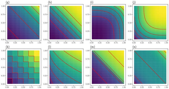
Figure 12: For $d=2$, the contour lines (red) of the regression functions corresponding to the functions $f$ in Table 2 at the levels $k/6$ for $k\in[5]$ are shown. The fill colour indicates the function value at the respective position from $0$ (purple) to $1$ (yellow).

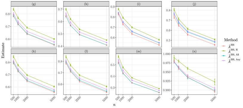
Figure 13: Estimates of $\mathbb{E}\bigl{\{}\mu\bigl{(}\mathcal{X}_{\tau}(\eta)\setminus\hat{A}\bigr{)}\bigr{\}}$ for $d=2$ and $\sigma=1/4$.

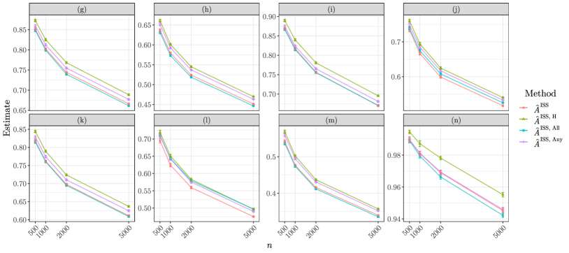
Figure 14: Estimates of $\mathbb{E}\bigl{\{}\mu\bigl{(}\mathcal{X}_{\tau}(\eta)\setminus\hat{A}\bigr{)}\bigr{\}}$ for $d=3$ and $\sigma=1/16$.

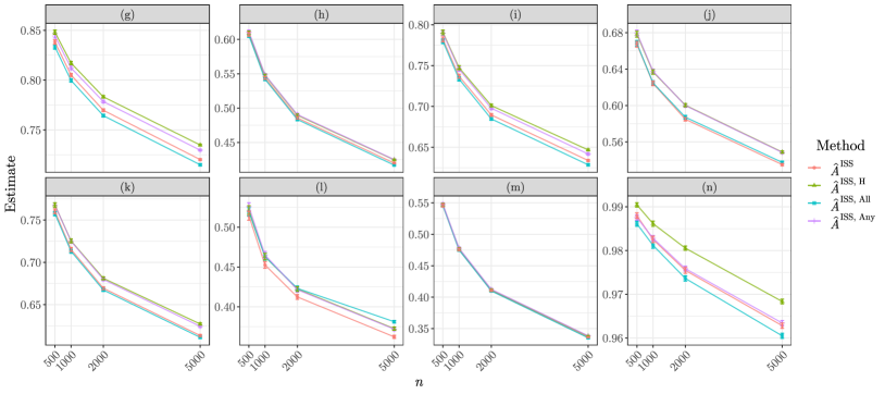
Figure 15: Estimates of $\mathbb{E}\bigl{\{}\mu\bigl{(}\mathcal{X}_{\tau}(\eta)\setminus\hat{A}\bigr{)}\bigr{\}}$ for $d=4$ and $\sigma=1/64$.

We now consider a comparison of $\hat{A}^{\mathrm{ISS}}$ with two possible procedures based on sample splitting. Indeed, a natural approach to combining our $p$-values is to employ a fixed sequence testing procedure (Hsu and Berger,, 1999; Westfall and Krishen,, 2001) as we do in the univariate setting in Section 3.2. However, since our sequence must be specified independently of the data used for testing, and there is no canonical total ordering in the multivariate case, sample splitting offers a potential way forward. We consider two such procedures: in the first, denoted $\hat{A}^{\mathrm{Split}}$, we use the first half of the data to compute $p$-values at each of our $n$ data points. These are then ordered from smallest to largest, and this determines the ordering for our fixed sequence testing based on $p$-values computed on the second half of the data. The second procedure, denoted $\hat{A}^{\mathrm{Split},\mathrm{OR}}$, discards the first half of the data and instead uses an oracle ordering of the data points using the underlying knowledge of the regression function; the second stage of the procedure is then identical to $\hat{A}^{\mathrm{Split}}$. Results comparing $\hat{A}^{\mathrm{ISS}}$ with $\hat{A}^{\mathrm{Split}}$ and $\hat{A}^{\mathrm{Split},\mathrm{OR}}$ are presented in Figures 16 and 17, which indicate that both of these sample-splitting variants have considerably worse empirical performance than $\hat{A}^{\mathrm{ISS}}$. This is perhaps surprising given the impressive numerical results for sample splitting in conjunction with fixed sequence testing reported by Angelopoulos et al., (2021). However, the performance of sample-splitting approaches is highly dependent on the procedure used to determine the ordering of the hypotheses from the first split of the data. Even exact knowledge of the regression function may be insufficient to determine an ordering with high conditional power, as the distribution of the $p$-values on the second half of the data also depends on the marginal distribution of the covariates. This is reflected in the fact that $\hat{A}^{\mathrm{Split},\mathrm{OR}}$ has worse performance than $\hat{A}^{\mathrm{Split}}$ in some cases, especially when the regression function depends only on a strict subset of the $d$ variables, such as case (l) in Figure 17.

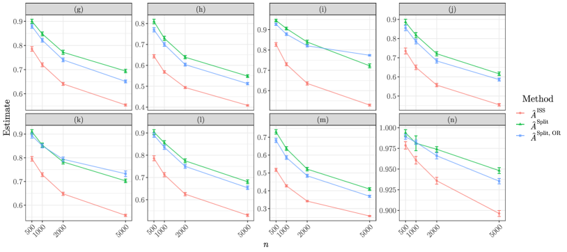
Figure 16: Estimates of $\mathbb{E}\bigl{\{}\mu\bigl{(}\mathcal{X}_{\tau}(\eta)\setminus\hat{A}\bigr{)}\bigr{\}}$ for $d=2$ and $\sigma=1/4$.

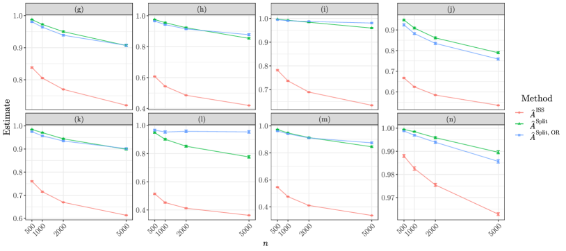
Figure 17: Estimates of $\mathbb{E}\bigl{\{}\mu\bigl{(}\mathcal{X}_{\tau}(\eta)\setminus\hat{A}\bigr{)}\bigr{\}}$ for $d=4$ and $\sigma=1/64$.

B.2 Computation time

In Figures 18 and 19, we present the average computation time of the different procedures studied in Section 5 for dimensions $d=2,4$ and regression functions (g)–(n) above. These reveal that the computation time varies quite substantially across the different regression functions but does not even necessarily increase at all with dimension. These effects are related to the depth of the DAG induced by the observations as well as the power of the procedures in the different settings.

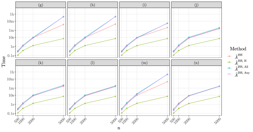
Figure 18: Computation time of the different estimates of $\mathbb{E}\bigl{\{}\mu\bigl{(}\mathcal{X}_{\tau}(\eta)\setminus\hat{A}\bigr{)}\bigr{\}}$ for $d=2$ and $\sigma=1/4$.

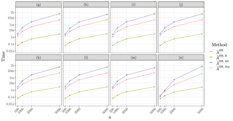
Figure 19: Computation time of the different estimates of $\mathbb{E}\bigl{\{}\mu\bigl{(}\mathcal{X}_{\tau}(\eta)\setminus\hat{A}\bigr{)}\bigr{\}}$ for $d=4$ and $\sigma=1/64$.

Appendix C Comparison with procedure based on Meijer & Goeman (2015)

As discussed in Section 2, our proposed procedure consists of two steps; calculating $p$-values to test whether the regression function $\eta$ exceeds the threshold $\tau$ at $m$ given points and then controlling the FWER over $\mathcal{P}_{\mathrm{Mon},d}(\sigma)$ through a DAG testing procedure. For the second step, an alternative approach would be to use the algorithm introduced by Meijer and Goeman, (2015). Indeed, the empirical results in Section 5 suggest that such a procedure can work well in some cases. However, we show in this section that it fails to attain the optimal worst-case regret over $\mathcal{P}_{\mathrm{Mon},d}(\sigma)\cap\mathcal{P}_{\mathrm{Reg},d}(\tau,\theta,\gamma,\lambda)$.

C.1 Description of procedure

The iterative algorithm of Meijer and Goeman, (2015) is an application of the sequential rejection principle (Goeman and Solari,, 2010) to hypotheses indexed by elements of $I=[m]$, for some $m\in\mathbb{N}$, that are a priori arranged as a DAG $G=(I,E)$. Inputs to the algorithm include a fixed significance level $\alpha\in(0,1)$, a vector $\bm{v}\in(0,\infty)^{m}$ and $(p_{i})_{i\in I}\in(0,1]^{m}$, with the latter thought of as a collection of $p$-values. Any choice of $\bm{v}$ will correspond to a DAG testing procedure, as defined by Definition 3. Each iteration of the procedure comprises three steps: the first assigns to each unrejected hypothesis (or, equivalently, the corresponding node) a proportion $\alpha_{i}$ of the $\alpha$-budget; the second step rejects any hypothesis $i\in I$ for which $p_{i}\leq\alpha_{i}$; and the third rejects all ancestors of rejected hypotheses. The procedure terminates if no new rejections are made in the second step of an iteration or if every hypothesis has been rejected, and hence takes at most $m$ iterations. In more detail, in the first step, the $\alpha$-budget is split among the unrejected leaf nodes in proportion to the corresponding elements of $\bm{v}$. These budgets are then propagated from the leaf nodes towards currently unrejected ancestor nodes. Meijer and Goeman, (2015) suggest two variants for this, which we enumerate by $\omega\in\{0,1\}$ and call the all-parent variant ($\omega=0$) and the any-parent variant ($\omega=1$). In the all-parent variant of the procedure, a node’s entire budget is evenly distributed among its unrejected parents (keeping nothing for itself), whereas in the any-parent variant, the budget that would go to rejected parents if it were evenly distributed among all parents simply stays at the node and only the remaining budget is evenly distributed among the unrejected parents. Importantly, the order in which the nodes pass their budgets to their parents follows a reverse topological ordering of $G$; all reverse topological orderings $\pi_{G}$ lead to the same output in Algorithm 3, making the specific choice immaterial. Thus, a node only distributes its budget once all of its descendants have distributed theirs. Once this budget propagation has terminated, we move to the second step and reject all hypotheses whose $p$-value does not exceed the assigned budget. Finally, the third step is only relevant in the any-parent variant of the procedure, and rejecting the ancestors of nodes rejected at the second step does not increase the Type I error rate when $G$ is $G_{0}$-consistent for a directed graph $G_{0}$ encoding all logical relationships between hypotheses (see Section 3.1). A concise formal description of the Meijer and Goeman, (2015) procedure, which outputs a set $\mathcal{R}_{\alpha}^{\mathrm{MG},\omega,\bm{v}}(G,\bm{p})$ of rejected hypotheses, is given in Algorithm 3.

Meijer and Goeman, (2015) prove that Algorithm 3 satisfies the two sufficient conditions for controlling the FWER described by Goeman and Solari, (2010). The DAG testing procedures $\mathcal{R}^{\mathrm{MG},\omega,\bm{v}}$ for $\omega\in\{0,1\}$ motivate the following selection sets

$$\hat{A}^{\mathrm{ISS},\omega} \phantom{:}\equiv\hat{A}^{\mathrm{ISS},\omega,\bm{v}}_{\sigma,\tau,\alpha,m}(\mathcal{D})$$

$$:=\bigl{\{}x\in\mathbb{R}^{d}:\!X_{i_{0}}\preccurlyeq x\text{ for some }i_{0}\in\mathcal{R}_{\alpha}^{\mathrm{MG},\omega,\bm{v}}\bigl{(}\mathcal{G}_{\mathrm{W}}(\mathcal{D}_{X,m}),\bigl{(}\hat{p}_{\sigma,\tau}(X_{i},\mathcal{D})\bigr{)}_{i\in[m]}\bigr{)}\bigr{\}}.$$

Indeed, by a proof analogous to that of Theorem 9, we have $\mathbb{P}_{P}\bigl{(}\hat{A}^{\mathrm{ISS},\omega,\bm{v}}_{\sigma,\tau,\alpha,m}(\mathcal{D})\subseteq\mathcal{X}_{\tau}(\eta)|\mathcal{D}_{X}\bigr{)}\geq 1-\alpha$ whenever $P\in\mathcal{P}_{\mathrm{Mon},d}(\sigma)$. However, the budget propagation mechanism in the first step of each iteration has an important drawback: if $I_{0}\subseteq I$ is such that there exists $i_{*}\in I$ with $\{i_{*}\}=\operatorname{\mathrm{ch}}_{G}(i)$ for all $i\in I_{0}$, then the sum of the budgets assigned to the nodes in $I_{0}$ can never exceed the budget that passes through node $i_{*}$. Moreover, the same conclusion holds for ancestors of nodes in $I_{0}$ that do not have descendants belonging to an antichain with $i_{*}$. Intuitively, this can make $i_{*}$ a bottleneck in the sense that the potentially large number of hypotheses $I_{0}$ may each only receive a fraction of the budget propagated through $i_{*}$.

Input: $\omega\in\{0,1\}$, $\alpha\in(0,1)$, $m\in\mathbb{N}$, a weighted DAG $G=([m],E,\bm{w})$, $\bm{p}=(p_{i})_{i\in[m]}\in(0,1]^{m}$, $\bm{v}=(v_{i})_{i\in[m]}\in(0,\infty)^{m}$

$\pi_{G}\leftarrow$ a topological ordering of $G$

$R^{\omega}_{0}\leftarrow\emptyset$

for $\ell\in[m]$ do

      

      $S_{\mathrm{L}}\leftarrow L(G)\setminus R^{\omega}_{\ell-1}$ // $S_{\mathrm{L}}$ is the set of currently unrejected leaf nodes

       $v_{i}^{*}\leftarrow v_{i}/\bigl{(}\sum_{i^{\prime}\in S_{\mathrm{L}}}v_{i^{\prime}}\bigr{)}$ for all $i\in S_{\mathrm{L}}$

       $\alpha_{\ell,0}^{\omega}(i)\leftarrow\mathbbm{1}_{\{i\in S_{\mathrm{L}}\}}\cdot\alpha\cdot v^{*}_{i}$ for all $i\in[m]$

       // iteratively distribute the $\alpha$-budget:

       for $k\in[m]$ do

             $i\leftarrow\pi_{G}^{-1}(k)$ // iterate through the nodes in order

             $R_{\mathrm{P}}\leftarrow\operatorname{\mathrm{pa}}_{G}(i)\cap R^{\omega}_{\ell-1}$ // currently rejected parents of node $i$

             $S_{\mathrm{P}}\leftarrow\operatorname{\mathrm{pa}}_{G}(i)\setminus R^{\omega}_{\ell-1}$ // currently unrejected parents of node $i$

            

            if $S_{\mathrm{P}}\neq\emptyset$ then

                  

                  if $\omega=0$ then

                         // evenly distribute the entire $\alpha$-budget among nodes in $S_{\mathrm{P}}$:

                         $\alpha_{\ell,k}^{\omega}(j)\leftarrow\alpha_{\ell,k-1}^{\omega}(j)+\frac{\alpha_{\ell,{k-1}}^{\omega}(i)}{|S_{\mathrm{P}}|}$ for all $j\in S_{\mathrm{P}}$

                         // no $\alpha$-budget remains in the node $i$ itself:

                         $\alpha_{\ell,k}^{\omega}(i)\leftarrow 0$

                        

                   else

                         // divide $\alpha$-budget among $R_{\mathrm{P}}\cup S_{\mathrm{P}}$, but only distribute to $S_{\mathrm{P}}$:

                         $\alpha_{\ell,k}^{\omega}(j)\leftarrow\alpha_{\ell,k-1}^{\omega}(j)+\frac{\alpha_{\ell,{k-1}}^{\omega}(i)}{|\operatorname{\mathrm{pa}}_{G}(i)|}$ for all $j\in S_{\mathrm{P}}$

                         // keep the $\alpha$-budget that would go to nodes in $R_{\mathrm{P}}$ in node $i$:

                         $\alpha_{\ell,k}^{\omega}(i)\leftarrow|R_{\mathrm{P}}|\cdot\frac{\alpha_{\ell,{k-1}}^{\omega}(i)}{|\operatorname{\mathrm{pa}}_{G}(i)|}$

                        

                   end if

                  

             else

                  

                  $\alpha_{\ell,k}^{\omega}(i)\leftarrow\alpha_{\ell,k-1}^{\omega}(i)$

                  

             end if

            

       end for

      

      $\alpha_{\ell}^{\omega}(i)\leftarrow\alpha_{\ell,m}^{\omega}(i)$ for all $i\in[m]$

       // reject nodes based on the final distribution of the $\alpha$-budget:

       $N\leftarrow\{i\in[m]:p_{i}\leq\alpha_{\ell}^{\omega}(i)\}$

       if $\omega=1$ then

            $N\leftarrow N\cup\bigcup_{i\in N}\operatorname{\mathrm{an}}_{G}(i)$

       end if

      if $N=\emptyset$ then

             $R^{\omega}_{m}\leftarrow R^{\omega}_{\ell-1}$

             break

            

       end if

      $R^{\omega}_{\ell}\leftarrow R^{\omega}_{\ell-1}\cup N$

      

end for

Result: The set of rejected hypotheses $\mathcal{R}^{\mathrm{MG},\omega,\bm{v}}_{\alpha}(G,\bm{p}):=R^{\omega}_{m}$

Algorithm 3 The Meijer and Goeman, (2015) one-way logical relation DAG testing procedure $\mathcal{R}^{\mathrm{MG}}$.

C.2 Sub-optimal worst-case performance

The following proposition illustrates that using the Meijer and Goeman, (2015) procedure in our setting leads to a sub-optimal worst-case rate, as seen by comparison with the upper bound for $\hat{A}^{\mathrm{ISS}}$ established in Theorem 15.

Proposition 37.

Let $d\geq 2$, $\tau\in\mathbb{R}$, $\sigma,\gamma,\lambda>0$, $\theta\in[2^{d},\infty)$, $\alpha\in(0,1/4]$ and $\omega\in\{0,1\}$. There exists $c>0$, depending only on $d$, $\alpha$, $\sigma$, $\lambda$ and $\gamma$, such that for every $n\in\mathbb{N}$,

$$\min_{m\in[n]}\sup_{P\in\mathcal{P}^{\prime}}\inf_{\bm{v}\in(0,\infty)^{m}}\mathbb{E}_{P}\bigl{\{}\mu\bigl{(}\mathcal{X}_{\tau}(\eta)\setminus\hat{A}^{\mathrm{ISS},\omega,\bm{v}}_{\sigma,\tau,\alpha,m}(\mathcal{D})\bigr{)}\bigr{\}}\geq\frac{c}{n^{1/(2\gamma+d+1)}(\log_{+}n)^{2/d}},$$

where $\mathcal{P}^{\prime}:=\mathcal{P}_{\mathrm{Mon},d}(\sigma)\cap\mathcal{P}_{\mathrm{Reg},d}(\tau,\theta,\gamma,\lambda)$.

(a) The support of $\mu$ and the shape of the $\tau$- and $(\tau+\epsilon)$-superlevel set of $\eta$ for $\epsilon\in[0,\lambda/2^{\gamma}]$ in the case $d=2$.

(b) The DAG induced by the points in $\mathcal{D}_{X,m}$ in Lemma 43 for any $d\geq 2$. Note $i_{q}=i_{1}^{*}$. See also the proof of Lemma 43 for notation.

Figure 20: Illustration of the probability distribution defined in Section C.2 and the resulting induced graph. The construction demonstrates a problematic consequence of the bottleneck effect described at the end of Section C.1: in order to identify the superlevel set, we need to reject nodes in $I_{A}$, but unless rejections have been made in previous iterations of Algorithm 3, the combined budget of the nodes in $I_{A}$ cannot exceed what is passed through $i_{q}$, which will be very little, as most is propagated towards $i_{2}^{*}$.

The main idea of the proof of Proposition 37 is to construct a distribution in $\mathcal{P}_{\mathrm{Mon},d}(\sigma)\cap\mathcal{P}_{\mathrm{Reg},d}(\tau,\theta,\gamma,\lambda)$, for which the Meijer and Goeman, (2015) algorithm propagates little budget to points in the $\tau$-superlevel set of the regression function $\eta$. This distribution, which belongs to $\mathcal{P}_{\mathrm{Mon},d}(\sigma)\cap\mathcal{P}_{\mathrm{Reg},d}(\tau,\theta,\gamma,\lambda)$ (Lemma 38), is illustrated in Figure 20. It consists of $q$ pairs of atoms, where the regression function $\eta$ is well below $\tau$, as well as an absolutely continuous component, where $\eta$ is at least $\tau$ (see Figure 20(a)). The probability masses at each atom are sufficiently large to ensure that, with high probability, we see at least one observation at each of them (Lemma 39). On this high probability event, the observations therefore induce the DAG illustrated in Figure 20(b). Moreover, the regression function at $i_{2}^{*}$ and $i_{q}$ is sufficiently below $\tau$ that the corresponding $p$-values exceed $\alpha$ with high probability (Lemma 40). At the same time, the marginal distribution and regression function on the set $A$ in Figure 20(a) are chosen so that all of the $p$-values corresponding to points in $A\setminus A_{\epsilon}$ exceed $\alpha/2^{q-1}$ with high probability (Lemmas 41 and 42). But, as we argue in Lemma 43, the budget propagation of the Meijer and Goeman, (2015) procedure means that a budget of at most $\alpha/2^{q-1}$ is passed into $A$. It then follows that with high probability, we can only reject hypotheses corresponding to points in $A_{\epsilon}$, and in that case the corresponding data-dependent selection set returned will omit $A\setminus A_{\epsilon}$. These ideas establish the result when $n$ and $m$ are sufficiently large; when $n$ is small, we can apply our earlier bound in Theorem 17 and when $m$ is small we can apply Proposition 44, which provides a lower bound for the worst-case performance of any data-dependent selection set that returns the upper hull of $m$ observations.

To begin our construction, let $A:=[0,1/2]\times[1/2,1]\times[0,1/2]^{d-2}$ and $q\in\mathbb{N}$. For $\bm{j}=(j_{1},j_{2})^{\top}\in\{1,2\}\times[q]$, define

$$z_{\bm{j}}:=\biggl{(}j_{1}-1,\frac{j_{2}}{2q}-1,0\ldots,0\biggr{)}^{\top}\in\mathbb{R}^{d}.$$ (16)

For $d\geq 2$ and $q\in\mathbb{N}$, let $\mu_{q}$ denote the distribution on $\mathbb{R}^{d}$ satisfying:

• $\mu_{q}(\{z_{\bm{j}}\})=(2^{d}-1)/(2^{d+1}q)$ for all $\bm{j}\in\{1,2\}\times[q]$;

• $\mu_{q}(A)=1/2^{d}$;

• $X|X\in A\sim\mathrm{Unif}(A)$ when $X\sim\mu_{q}$.

Thus $\sum_{\bm{j}\in\{1,2\}\times[q]}\mu_{q}(\{z_{\bm{j}}\})=1-1/2^{d}$ and $\mu_{q}(B\cap A)=\mathcal{L}_{d}(B\cap A)$ for any Borel set $B\subseteq\mathbb{R}^{d}$. Write $x_{A}:=(0,1/2,0,\ldots,0)^{\top}\in\mathbb{R}^{d}$, so that $x_{A}\in A$ and $x\succcurlyeq x_{A}$ for all $x\in A$. For $q\in\mathbb{N}$, $M>0$, $\tau\in\mathbb{R}$, $\gamma,\lambda>0$ define $\eta_{q,M}\equiv\eta_{q,M,\tau,\lambda,\gamma}:\mathbb{R}^{d}\rightarrow\mathbb{R}$ by

$$\eta_{q,M}(x^{(1)},\ldots,x^{(d)}):=\begin{cases}\tau+\lambda\cdot\min_{j\in[d]}\bigl{(}x^{(j)}-x_{A}^{(j)}\bigr{)}^{\gamma}&\quad\text{ if }x\succcurlyeq x_{A}\\ \tau-M&\quad\text{ otherwise},\end{cases}$$

where $x_{A}^{(j)}$ denotes the $j$th coordinate of $x_{A}$. Finally, for $q\in\mathbb{N}$, $M>0$, $\sigma>0$, $\tau\in\mathbb{R}$, $\gamma,\lambda>0$, let $P_{q,M}\equiv P_{q,M,\sigma,\tau,\lambda,\gamma}$ denote any joint distribution of $(X,Y)$ such that $X$ has marginal distribution $\mu_{q}$, and $Y|X\sim\mathcal{N}\bigl{(}\eta_{q,M}(X),\sigma^{2}\bigr{)}$.

Lemma 38.

For $d\geq 2$, $\tau\in\mathbb{R}$, $\sigma,\gamma,\lambda>0$, $q\in\mathbb{N}$ and $M>0$, we have $P_{q,M}\equiv P_{q,M,\sigma,\tau,\lambda,\gamma}\in\mathcal{P}_{\mathrm{Mon},d}(\sigma)\cap\mathcal{P}_{\mathrm{Reg},d}(\tau,\theta,\gamma,\lambda)$ for all $\theta\geq 2^{d}$.

Proof.

We first prove that $P_{q,M}\in\mathcal{P}_{\mathrm{Mon},d}(\sigma)$. Since the sub-Gaussianity condition is satisfied by construction, it suffices to show that $\eta_{q,M}$ is coordinate-wise increasing on $\mathbb{R}^{d}$. Whenever $x_{0}\not\succcurlyeq x_{A}$, we have $\eta_{q,M}(x_{0})=\inf_{x\in\mathbb{R}^{d}}\eta_{q,M}(x)$. On the other hand, for $x_{0},x_{1}\in\mathbb{R}^{d}$ with $x_{A}\preccurlyeq x_{0}\preccurlyeq x_{1}$, we have

$$\eta_{q,M}(x_{0})=\tau+\lambda\cdot\min_{j\in[d]}\bigl{(}x_{0}^{(j)}-x_{A}^{(j)}\bigr{)}^{\gamma}\leq\tau+\lambda\cdot\min_{j\in[d]}\bigl{(}x_{1}^{(j)}-x_{A}^{(j)}\bigr{)}^{\gamma}=\eta_{q,M}(x_{1}),$$

as required.

We now show that $P_{q,M}\in\mathcal{P}_{\mathrm{Reg},d}(\tau,\theta,\gamma,\lambda)$ and start by establishing that the condition in Definition 13(i) is satisfied. For any $x\in\mathcal{X}_{\tau}(\eta)\cap\mathrm{supp}(\mu_{q})=A$ and $r\in(0,1]$, we have $\mu_{q}\bigl{(}{B}_{\infty}(x,r)\bigr{)}\geq\bigl{(}r\wedge(1/2)\bigr{)}^{d}\geq(r/2)^{d}$. For $r\geq 1/4^{d}$, we have $\mu_{q}\bigl{(}{B}_{\infty}(x,r)\bigr{)}\leq 1\leq\theta\cdot(2r)^{d}$, so let $r\in(0,1/4^{d})$. We then have for any $x\in A$ that ${B}_{\infty}(x,r)\cap\bigcup_{\bm{j}\in\{1,2\}\times[q]}\{z_{\bm{j}}\}=\emptyset$ and hence $\mu_{q}\bigl{(}{B}_{\infty}(x,r)\bigr{)}=\mu_{q}\bigl{(}{B}_{\infty}(x,r)\cap A\bigr{)}\leq(2r)^{d}$. Finally, for Definition 13(ii), observe that for any $x\in\mathcal{X}_{\tau}(\eta)\cap\mathrm{supp}(\mu_{q})=A$ and $r\in(0,1]$, we have $x_{0}:=x+r\bm{1}_{d}\in{B}_{\infty}(x,r)$ satisfies $x_{0}-x_{A}\succcurlyeq r\bm{1}_{d}$ and hence $\eta_{q,M}(x_{0})\geq\tau+\lambda r^{\gamma}$, as required. ∎

Lemma 39.

Fix $d\geq 2$, $\delta\in(0,1)$, positive integers $m\leq n$ and $q\leq\bigl{\lfloor}\frac{m}{32\log_{+}(m/\delta)}\bigr{\rfloor}$. If $\mathcal{D}_{X,m}=\bigl{(}X_{1},\ldots,X_{m}\bigr{)}\sim\mu_{q}^{m}$, and we define $\Omega_{1}:=\bigcap_{\bm{j}\in\{1,2\}\times[q]}\bigl{\{}\{z_{\bm{j}}\}\cap\mathcal{D}_{X,m}\neq\emptyset\bigr{\}}$, then $\mathbb{P}_{\mu_{q}}(\Omega_{1}^{c})\leq\delta/4$.

Proof.

For $\bm{j}\in\{1,2\}\times[q]$, let

$$\Omega_{1,\bm{j}}:=\biggl{\{}\frac{1}{m}\sum_{i=1}^{m}\mathbbm{1}_{\{X_{i}=z_{\bm{j}}\}}\geq\frac{2^{d}-1}{2^{d+2}q}\biggr{\}}.$$

Then by the multiplicative Chernoff bound (McDiarmid,, 1998, Theorem 2.3(c)), the fact that $(2^{d}-1)/2^{d+4}\geq 1/32$ and the choice of $q$, we have

$$\mathbb{P}_{\mu_{q}}\biggl{(}\bigcup_{\bm{j}\in\{1,2\}\times[q]}\Omega^{c}_{1,\bm{j}}\biggr{)}\leq 2q\cdot\exp\biggl{(}-\frac{2^{d}-1}{2^{d+4}q}\cdot m\biggr{)}\leq\frac{m}{4}\cdot\exp\Bigl{\{}-\log_{+}\Bigl{(}\frac{m}{\delta}\Bigr{)}\Bigr{\}}\leq\frac{\delta}{4}.$$

Moreover,

$$\frac{(2^{d}-1)m}{2^{d+2}q}\geq\frac{m}{8q}\geq 4\log_{+}(m/\delta)\geq 1,$$

whence

$$\mathbb{P}_{\mu_{q}}\bigl{(}\Omega_{1}^{c}\bigr{)}=\mathbb{P}_{\mu_{q}}\biggl{(}\bigcup_{\bm{j}\in\{1,2\}\times[q]}\biggl{\{}\frac{1}{m}\sum_{i=1}^{m}\mathbbm{1}_{\{X_{i}=z_{\bm{j}}\}}=0\biggr{\}}\biggr{)}\leq\mathbb{P}_{\mu_{q}}\biggl{(}\bigcup_{\bm{j}\in\{1,2\}\times[q]}\Omega_{1,\bm{j}}^{c}\biggr{)}\leq\frac{\delta}{4},$$

as required. ∎

Lemma 40.

Fix $d\geq 2$, $\alpha\in(0,1)$, $\delta\in(0,1]$, $n\in\mathbb{N}$, $m\in[n]$, $\tau\in\mathbb{R}$, $\sigma,\gamma,\lambda>0$, $q\in\mathbb{N}$ and $M\geq 1.7\sigma\sqrt{\log(41.6/\delta)}$. Let $\mathcal{D}=\bigl{(}(X_{1},Y_{1}),\ldots,(X_{n},Y_{n})\bigr{)}\sim P_{q,M}^{n}$, and suppose that $\bigl{\{}i\in[m]:X_{i}=z_{(j,q)}\bigr{\}}\neq\emptyset$ for $j\in\{1,2\}$. Write $i^{*}_{j}:=\max\{i\in[m]:X_{i}=z_{(j,q)}\}$ for $j\in\{1,2\}$, and let

$$\Omega_{2}:=\bigcap_{j=1}^{2}\bigl{\{}\hat{p}_{\sigma,\tau}(X_{i^{*}_{j}},\mathcal{D})>\alpha\bigr{\}}.$$

Then $\mathbb{P}_{P_{q,M}}\bigl{(}\Omega_{2}^{c}|\mathcal{D}_{X}\bigr{)}\leq\delta/4$.

Proof.

For $x\in\mathbb{R}^{d}$ and $r>0$, define $\mathcal{I}_{r}(x):=\{i\in[n]:X_{i}\preccurlyeq x,\|X_{i}-x\|_{\infty}\leq r\}$. Fix $j\in\{1,2\}$, and note that

$$\frac{\sigma}{|\mathcal{I}_{r}(X_{i^{*}_{j}})|}\cdot u_{\delta/8}\bigl{(}|\mathcal{I}_{r}(X_{i^{*}_{j}})|\bigr{)} \leq 1.7\sigma\sqrt{0.2+0.72\log(41.6/\delta)}\leq 1.7\sigma\sqrt{\log(41.6/\delta)}\leq M$$

for all $r>0$. It follows by Lemma 45(a) that, with probability at least $1-\delta/8$ given $\mathcal{D}_{X}$, we have simultaneously for all $r>0$ that

$$\sum_{i\in\mathcal{I}_{r}(X_{i^{*}_{j}})}\frac{Y_{i}-\tau}{\sigma} =\sum_{i\in\mathcal{I}_{r}(X_{i^{*}_{j}})}\frac{Y_{i}-(\tau-M)}{\sigma}-|\mathcal{I}_{r}(X_{i^{*}_{j}})|\cdot\frac{M}{\sigma}$$

$$\leq u_{\delta/8}\bigl{(}|\mathcal{I}_{r}(X_{i^{*}_{j}})|\bigr{)}-|\mathcal{I}_{r}(X_{i^{*}_{j}})|\cdot\frac{M}{\sigma}\leq 0,$$

so that $\hat{p}_{\sigma,\tau}(X_{i^{*}_{j}},\mathcal{D})=1$, and thus in particular $\hat{p}_{\sigma,\tau}(X_{i^{*}_{j}},\mathcal{D})>\alpha$. Hence, the result follows by a union bound over $j\in\{1,2\}$. ∎

Lemma 41.

Fix $d\geq 2$, $\alpha\in(0,1)$, $\delta\in(0,1/4]$, $n\in\mathbb{N}$, $\sigma,\gamma,\lambda>0$, $s\in(0,1/2]$ and $q\in\mathbb{N}$. Let $\mathcal{D}_{X}=(X_{1},\ldots,X_{n})\sim\mu_{q}^{n}$ and let $B_{j}:=x_{A}+[0,1/2]^{j-1}\times[0,s]\times[0,1/2]^{d-j}$ for $j\in[d]$. Denote $w_{n,m,\delta}:=173.13\bigl{(}\log_{+}\log n+\log_{+}(m/\delta)\bigr{)}$. If

$$\frac{8}{3n}\log\Bigl{(}\frac{4d}{\delta}\Bigr{)}\leq\frac{s}{2^{d-1}}\leq\frac{\sigma^{2}}{2n\lambda^{2}s^{2\gamma}}\bigl{(}0.72q-w_{n,m,\delta}\bigr{)}$$

then, writing

$$\Omega_{3}:=\bigcap_{j\in[d]}\biggl{\{}|\mathcal{D}_{X}\cap B_{j}|<\frac{\sigma^{2}}{\lambda^{2}s^{2\gamma}}\bigl{(}0.72q-w_{n,m,\delta}\bigr{)}\biggr{\}},$$

we have $\mathbb{P}_{\mu_{q}}(\Omega_{3}^{c})\leq\delta/4$.

Proof.

Fix any $j\in[d]$ and note that $\mu_{q}(B_{j})=s/2^{d-1}$. By the upper bound on $s$, a multiplicative Chernoff bound (McDiarmid,, 1998, Theorem 2.3(b)) and the lower bound on $s$, we have

$$\mathbb{P}_{\mu_{q}}\Bigl{(}|\mathcal{D}_{X}\cap B_{j}|\geq\frac{\sigma^{2}}{\lambda^{2}s^{2\gamma}}\bigl{(}0.72q-w_{m,n,\delta}\bigr{)}\Bigr{)} \leq\mathbb{P}_{\mu_{q}}\Bigl{(}|\mathcal{D}_{X}\cap B_{j}|\geq\frac{ns}{2^{d-2}}\Bigr{)}$$

$$\leq\exp\Bigl{(}-\frac{3ns}{8\cdot 2^{d-1}}\Bigr{)}\leq\frac{\delta}{4d}.$$

The result therefore follows by a union bound. ∎

Lemma 42.

Fix $d\geq 2$, $\alpha\in(0,1)$, $\delta\in(0,1]$, $n\in\mathbb{N}$, $m\in[n]$, $\tau\in\mathbb{R}$, $\sigma,\gamma,\lambda>0$, $q\in\mathbb{N}$, $M>0$ and $s>0$. Let $\mathcal{D}=\bigl{(}(X_{1},Y_{1}),\ldots,(X_{n},Y_{n})\bigr{)}\sim P_{q,M}^{n}$, and let $1\leq i_{1}<\ldots<i_{K}\leq m$ be such that $\{i_{1},\ldots,i_{K}\}:=\bigl{\{}i\in[m]:X_{i}\in\mathcal{X}_{\tau}(\eta_{q,M})\setminus\mathcal{X}_{\tau+\lambda s^{\gamma}}(\eta_{q,M})\bigr{\}}$. Denote further $w_{n,m,\delta}:=173.13\bigl{(}\log_{+}\log n+\log_{+}(m/\delta)\bigr{)}$ as in Lemma 41. If $q\geq w_{n,m,\delta}/0.72\geq 3\log(5.2\cdot 8\cdot m/\delta)+2\log\log(2n)$ and

$$\max_{k\in[K]}\bigl{|}\{i\in[n]:X_{i}\in A,X_{i}\preccurlyeq X_{i_{k}}\}\bigr{|}\leq\frac{\sigma^{2}}{\lambda^{2}s^{2\gamma}}\bigl{(}0.72q-w_{n,m,\delta}\bigr{)}$$

then writing

$$\Omega_{4}:=\bigcap_{k\in[K]}\Bigl{\{}\hat{p}_{\sigma,\tau}(X_{i_{k}},\mathcal{D})>\frac{\alpha}{2^{q-1}}\Bigr{\}},$$

we have $\mathbb{P}_{P_{q,M}}\bigl{(}\Omega_{4}^{c}|\mathcal{D}_{X}\bigr{)}\leq\delta/4$.

Proof.

When $K=0$, i.e. $\bigl{\{}i\in[m]:X_{i}\in\mathcal{X}_{\tau}(\eta_{q,M})\setminus\mathcal{X}_{\tau+\lambda s^{\gamma}}(\eta_{q,M})\bigr{\}}=\emptyset$, then $\Omega_{4}^{c}=\emptyset$ and there is nothing to prove, so assume that $K\in[m]$. For $x\in\mathbb{R}^{d}$ and $r>0$, define $\mathcal{I}_{r}(x):=\{i\in[n]:X_{i}\preccurlyeq x,\|X_{i}-x\|_{\infty}\leq r\}$, $\mathcal{I}^{A}_{r}(x):=\{i\in\mathcal{I}_{r}(x):X_{i}\in A\}$ and accordingly $\mathcal{I}^{A^{c}}_{r}(x):=\{i\in\mathcal{I}_{r}(x):X_{i}\notin A\}$. Fix any $k\in[K]$ and note first that by assumption,

$$|\mathcal{I}^{A}_{r}(X_{i_{k}})|\leq\bigl{|}\{i\in[n]:X_{i}\in A,X_{i}\preccurlyeq X_{i_{k}}\}\bigr{|}\leq\frac{\sigma^{2}}{\lambda^{2}s^{2\gamma}}\bigl{(}0.72q-w_{n,m,\delta}\bigr{)}$$

for all $r>0$. Hence

$$\frac{\lambda^{2}s^{2\gamma}}{\sigma^{2}}\bigl{|}\mathcal{I}^{A}_{r}(X_{i_{k}})\bigr{|}^{2} \leq\bigl{|}\mathcal{I}^{A}_{r}(X_{i_{k}})\bigr{|}\cdot\bigl{(}0.72q-w_{n,m,\delta}\bigr{)}$$

$$\leq\frac{|\mathcal{I}_{r}(X_{i_{k}})|}{2}\biggl{\{}2.0808\cdot q\cdot\log 2-6\cdot 1.7^{2}\cdot\log_{+}\log n$$

$$\hskip 184.9429pt-4\cdot 1.7^{2}\cdot 0.72\cdot 5.2\cdot 8\cdot\log_{+}\Bigl{(}\frac{m}{\delta}\Bigr{)}\biggr{\}}$$

$$\leq\frac{|\mathcal{I}_{r}(X_{i_{k}})|}{2}\biggl{\{}2.0808\log\Bigl{(}\frac{5.2}{\alpha}\cdot 2^{q-1}\Bigr{)}+\Bigl{(}1.7^{2}-4\cdot 1.7^{2}\Bigr{)}\log\log\bigl{(}2|\mathcal{I}_{r}(X_{i_{k}})|\bigr{)}$$

$$\hskip 184.9429pt-4\cdot 1.7^{2}\cdot 0.72\cdot\log\Bigl{(}\frac{5.2\cdot 8\cdot K}{\delta}\Bigr{)}\biggr{\}}$$

$$\leq|\mathcal{I}_{r}(X_{i_{k}})|\biggl{\{}\sqrt{1.7^{2}\cdot 0.72\log\Bigl{(}\frac{5.2}{\alpha}\cdot 2^{q-1}\Bigr{)}+1.7^{2}\log\log\bigl{(}2|\mathcal{I}_{r}(X_{i_{k}})|\bigr{)}}$$

$$\hskip 42.67912pt-\sqrt{2\cdot 1.7^{2}\log\log\bigl{(}2|\mathcal{I}_{r}(X_{i_{k}})|\bigr{)}+2\cdot 1.7^{2}\cdot 0.72\cdot\log\Bigl{(}\frac{5.2\cdot 8\cdot K}{\delta}\Bigr{)}}\biggr{\}}^{2}$$

$$=\Bigl{(}u_{\alpha/2^{q-1}}\bigl{(}|\mathcal{I}_{r}(X_{i_{k}})|\bigr{)}-\sqrt{2}\cdot u_{\delta/(8K)}\bigl{(}|\mathcal{I}_{r}(X_{i_{k}})|\bigr{)}\Bigr{)}^{2},$$ (17)

where in the final inequality, we used the fact that $(a-2b)/2\leq\bigl{(}\sqrt{a}-\sqrt{b}\bigr{)}^{2}$ for $a,b\geq 0$. By Lemma 45(a), with probability at least $1-\delta/(4K)$ conditional on $\mathcal{D}_{X}$, we have simultaneously for all $r>0$ that

$$\sum_{i\in\mathcal{I}_{r}(X_{i_{k}})}\frac{Y_{i}-\tau}{\sigma} \leq\sum_{i\in\mathcal{I}^{A}_{r}(X_{i_{k}})}\frac{Y_{i}-(\tau+\lambda s^{\gamma})}{\sigma}+\sum_{i\in\mathcal{I}^{A^{c}}_{r}(X_{i_{k}})}\frac{Y_{i}-(\tau-M)}{\sigma}+\frac{\lambda s^{\gamma}}{\sigma}|\mathcal{I}^{A}_{r}(X_{i_{k}})|$$

$$<u_{\delta/(8K)}\bigl{(}|\mathcal{I}^{A}_{r}(X_{i_{k}})|\bigr{)}+u_{\delta/(8K)}\bigl{(}|\mathcal{I}^{A^{c}}_{r}(X_{i_{k}})|\bigr{)}+\frac{\lambda s^{\gamma}}{\sigma}|\mathcal{I}^{A}_{r}(X_{i_{k}})|$$

$$\leq\sqrt{2}\cdot u_{\delta/(8K)}\bigl{(}|\mathcal{I}_{r}(X_{i_{k}})|\bigr{)}+\frac{\lambda s^{\gamma}}{\sigma}|\mathcal{I}^{A}_{r}(X_{i_{k}})|$$

$$\leq u_{\alpha/2^{q-1}}\bigl{(}|\mathcal{I}_{r}(X_{i_{k}})|\bigr{)},$$

where the third inequality follows from that fact that $\sqrt{a}+\sqrt{b}\leq\sqrt{2}\cdot\sqrt{a+b}$ for all $a,b\geq 0$, and the fourth follows from (C.2) and the fact that $u_{\alpha/2^{q-1}}\bigl{(}|\mathcal{I}_{r}(X_{i_{k}})|\bigr{)}\geq\sqrt{2}\cdot u_{\delta/(8K)}\bigl{(}|\mathcal{I}_{r}(X_{i_{k}})|\bigr{)}$ since $q\geq 3\log(5.2\cdot 8\cdot m/\delta)+2\log\log(2n)$. But

$$\biggl{\{}\sum_{i\in\mathcal{I}_{r}(X_{i_{k}})}\frac{Y_{i}-\tau}{\sigma}<u_{\alpha/2^{q-1}}\bigl{(}|\mathcal{I}_{r}(X_{i_{k}})|\bigr{)}\biggr{\}}=\bigl{\{}\hat{p}_{\sigma,\tau}(X_{i_{k}},\mathcal{D})>\alpha/2^{q-1}\bigr{\}},$$

so the result follows by a union bound over $k\in[K]$. ∎

Lemma 43.

Fix $m,q\in\mathbb{N}$ and suppose that $\mathcal{D}_{X,m}=\{X_{i}:i\in[m]\}\subseteq\bigl{\{}z_{\bm{j}}:\bm{j}\in\{1,2\}\times[q]\bigr{\}}\cup A$ with $\{z_{\bm{j}}\}\cap\mathcal{D}_{X,m}\neq\emptyset$ for all $\bm{j}\in\{1,2\}\times[q]$. Fix $\alpha\in(0,1)$ and let $(p_{i})_{i\in[m]}\in(0,1]^{m}$ be such that $\min_{j\in\{1,2\}}p_{i^{*}_{j}}>\alpha$, where $i^{*}_{j}:=\max\{i\in[m]:X_{i}=z_{(j,q)}\}$. Then for $\omega\in\{0,1\}$ and $\bm{v}\in(0,\infty)^{m}$, we have

$$\mathcal{R}^{\mathrm{MG},\omega,\bm{v}}_{\alpha}\bigl{(}\mathcal{G}_{\mathrm{W}}(\mathcal{D}_{X,m}),(p_{i})_{i\in[m]}\bigr{)}\cap\{i\in[m]:p_{i}>\alpha/2^{q-1}\text{ and }X_{i}\in A\}=\emptyset.$$

Proof.

Let $R_{0}^{\omega}:=\emptyset$, and for $\ell\in[m]$ and $k\in[m]\cup\{0\}$, let $R_{\ell}^{\omega}$, $\alpha^{\omega}_{\ell}$ and $\alpha_{\ell,k}^{\omega}$ be as in Algorithm 3. Furthermore, for ease of notation, let $I_{A}:=\{i\in[m]:X_{i}\in A\}$, $I_{\bm{j}}:=\{i\in[m]:X_{i}=z_{\bm{j}}\}$ for $\bm{j}\in\{1,2\}\times[q]$ and $I_{A^{c}}:=\{i\in[m]:X_{i}\notin A\}=\bigcup_{\bm{j}\in\{1,2\}\times[q]}I_{\bm{j}}$; see Figure 20(b). For each $\ell\in[m]\cup\{0\}$ let $P(\ell)$ denote the proposition that

$$R_{\ell}^{\omega}\cap\Bigl{(}\bigl{\{}i\in I_{A}:p_{i}>\alpha(1/2)^{q-1}\bigr{\}}\cup I_{A^{c}}\Bigr{)}=\emptyset.$$

Since $\mathcal{R}^{\mathrm{MG},\omega,\bm{v}}_{\alpha}\bigl{(}\mathcal{G}_{\mathrm{W}}(\mathcal{D}_{X,m}),(p_{i})_{i\in[m]}\bigr{)}=R_{m}^{\omega}$, the result will follow if $P(\ell)$ is true for all $\ell\in[m]\cup\{0\}$, and we prove this by induction on $\ell$. First, note that $P(0)$ is true since $R^{\omega}_{0}=\emptyset$. Now, fix any $\ell_{0}\in[m-1]\cup\{0\}$ such that $P(\ell_{0})$ holds true. In particular, this means that no hypothesis corresponding to a node in $I_{A^{c}}$ has been rejected in the first $\ell_{0}$ steps of the algorithm. For $j\in[q]$, define $i_{j}:=\max I_{(1,j)}$, so that $i_{q}=i_{1}^{*}$, and let $G:=\mathcal{G}_{\mathrm{W}}(\mathcal{D}_{X,m})$. Since $\mathrm{pa}_{G}(i)\subseteq I_{A^{c}}$ whenever $i\in I_{A^{c}}\setminus\{i_{1}^{*}\}$, we have that $P(\ell_{0}+1)$ is true if $i_{1}^{*},i_{2}^{*}\notin R^{\omega}_{\ell_{0}+1}$ and $\alpha^{\omega}_{\ell_{0}+1}(i)\leq\alpha/2^{q-1}$ for all $i\in I_{A}$. Regarding the first of these conditions, we have $\sum_{i\in[m]}\alpha^{\omega}_{\ell}(i)=\alpha$ for all $\ell\in[m]\cup\{0\}$, so in particular $\alpha^{\omega}_{\ell_{0}+1}(i_{j}^{*})\leq\alpha<p_{i_{j}^{*}}$ for $j\in\{1,2\}$ and hence $i_{1}^{*},i_{2}^{*}\notin R^{\omega}_{\ell_{0}+1}$. For the second condition, note that by definition, $L(G)=\{i_{\mathrm{L}}\}$ with $i_{\mathrm{L}}:=\min I_{(1,1)}$. There exists exactly one directed path from $i_{j}$ to $i_{\mathrm{L}}$, unless $j=1$ and $|I_{(1,1)}|=1$. Thus, for any $j\in[q]$, it follows that $k_{j}:=\min\bigl{\{}k\in[m]\cup\{0\}:\alpha_{\ell_{0}+1,k}^{\omega}(i_{j})>0\bigr{\}}$ is the maximiser of $k\mapsto\alpha_{\ell_{0}+1,k}^{\omega}(i_{j})$ over $k\in[m]\cup\{0\}$. We now claim that $\alpha_{\ell_{0}+1,k_{j}}^{\omega}(i_{j})=\alpha/2^{j-1}$ and show this by another induction, this time on $j\in[q]$. First, each node in $I_{(1,1)}\setminus\{i_{1}\}$ has exactly one parent and this parent is itself contained in $I_{(1,1)}$, so that $\alpha_{\ell_{0}+1,k_{1}}^{\omega}(i_{1})=\alpha_{\ell_{0}+1,0}^{\omega}(i_{\mathrm{L}})=\alpha$ for any $\bm{v}$. If $q=1$, this establishes the claim; otherwise, fix $j_{0}\in[q-1]$ for which $\alpha_{\ell_{0}+1,k_{j_{0}}}^{\omega}(i_{j_{0}})=\alpha/2^{j_{0}-1}$. By construction, $\operatorname{\mathrm{pa}}_{G}(i_{j_{0}})=\{\min I_{(1,j_{0}+1)},\min I_{(2,j_{0})}\}$ and each node in $I_{(1,j_{0}+1)}\setminus\{i_{j_{0}+1}\}$ has again exactly one parent, which is contained in $I_{(1,j_{0}+1)}$, while at the same time each node in $I_{(1,j_{0}+1)}\setminus\{\min I_{(1,j_{0}+1)}\}$ has exactly one child, which is also contained in $I_{(1,j_{0}+1)}$. Hence $\alpha_{\ell_{0}+1,k_{j_{0}+1}}^{\omega}(i_{j_{0}+1})=\alpha_{\ell_{0}+1,k_{j_{0}}}^{\omega}(i_{j_{0}})/2=\alpha(1/2)^{j_{0}}$, which completes the induction on $j\in[q]$. Since for any $i\in I_{A}$, any directed path in $G$ from $i$ to $i_{\mathrm{L}}$ necessarily contains $i_{q}$, we deduce that

$$\max_{i\in I_{A}}\alpha_{\ell_{0}+1}^{\omega}(i)\leq\sum_{i\in I_{A}}\alpha_{\ell_{0}+1}^{\omega}(i)\leq\alpha_{\ell_{0}+1,k_{q}}^{\omega}(i_{q})=\frac{\alpha}{2^{q-1}},$$

which completes the induction on $\ell\in[m]\cup\{0\}$ and hence the proof. ∎

For $m\in[n]$, let $\hat{\mathcal{A}}^{\mathrm{U}}_{n,m}(\tau,\alpha,\mathcal{P})\subseteq\hat{\mathcal{A}}_{n}(\tau,\alpha,\mathcal{P})$ denote the subfamily of data-dependent selection sets that control the Type I error at level $\alpha$ over $\mathcal{P}$ and for which $\hat{A}(\mathcal{D})$ is almost surely the upper hull of a subset of $\mathcal{D}_{X,m}$. Thus, for example, $\hat{A}^{\mathrm{ISS},\omega,\bm{v}}_{\sigma,\tau,\alpha,m}(\mathcal{D})\in\hat{\mathcal{A}}^{\mathrm{U}}_{n,m}\bigl{(}\tau,\alpha,\mathcal{P}_{\mathrm{Mon},d}(\sigma)\bigr{)}$ and $\hat{A}^{\mathrm{ISS}}_{\sigma,\tau,\alpha,m}(\mathcal{D})\in\hat{\mathcal{A}}^{\mathrm{U}}_{n,m}\bigl{(}\tau,\alpha,\mathcal{P}_{\mathrm{Mon},d}(\sigma)\bigr{)}$.

Proposition 44.

Fix $d\in\mathbb{N}$, $\alpha\in(0,1/4]$, $n\in\mathbb{N}$, $m\in[n]$, $\tau\in\mathbb{R}$, $\sigma,\gamma,\lambda>0$ and $\theta>1$. There exists $c\in(0,1)$, depending only on $d$, such that

$$\sup_{P\in\mathcal{P}^{\prime}}\inf_{\hat{A}\in\hat{\mathcal{A}}^{\mathrm{U}}_{n,m}(\tau,\alpha,\mathcal{P}^{\prime})}\mathbb{E}_{P}\bigl{\{}\mu\bigl{(}\mathcal{X}_{\tau}(\eta)\setminus\hat{A}(\mathcal{D})\bigr{)}\bigr{\}}\geq c\cdot\frac{1}{m^{1/d}},$$

where $\mathcal{P}^{\prime}:=\mathcal{P}_{\mathrm{Mon},d}(\sigma)\cap\mathcal{P}_{\mathrm{Reg},d}(\tau,\theta,\gamma,\lambda)$.

Proof.

For $q\in\mathbb{N}$, let the antichain $\mathbb{W}_{q,d}$, hypercubes $\mathcal{H}_{\bm{j}}^{q}$ for $\bm{j}\in\mathbb{W}_{q,d}$ as well as $P_{S}$, $\eta_{S}$ for $S\subseteq\mathbb{W}_{q,d}$ be defined as in Section A.3 and let $\mu:=\mathrm{Unif}\bigl{(}[0,1]^{d}\bigr{)}$. For ease of notation, we write $P_{*}:=P_{S}$ and $\eta_{*}:=\eta_{S}$ when $S=\mathbb{W}_{q,d}$. Note first that for any $\hat{A}\in\hat{\mathcal{A}}^{\mathrm{U}}_{n,m}(\tau,\alpha,\mathcal{P}^{\prime})$ we have on $\{\hat{A}(\mathcal{D})\subseteq\mathcal{X}_{\tau}(\eta_{*})\}$ that

$$\hat{S}:=\{\bm{j}\in\mathbb{W}_{q,d}:\hat{A}(\mathcal{D})\cap\mathcal{H}_{\bm{j}}^{q}\neq\emptyset\}\subseteq\{\bm{j}\in\mathbb{W}_{q,d}:\mathcal{D}_{X,m}\cap\mathcal{H}_{\bm{j}}^{q}\neq\emptyset\}=:\tilde{S}.$$

Now, for any $q\in\mathbb{N}$ and $\hat{A}\in\hat{\mathcal{A}}^{\mathrm{U}}_{n,m}(\tau,\alpha,\mathcal{P}^{\prime})$, we have $\mu\bigl{(}\mathcal{X}_{\tau}(\eta_{*})\setminus\hat{A}(\mathcal{D})\bigr{)}\geq|\mathbb{W}_{q,d}\setminus\hat{S}|/{q^{d}}$ and $|\mathbb{W}_{q,d}|\geq q^{d-1}/d$, so that

$$\mathbb{E}_{P_{*}}\bigl{\{}\mu\bigl{(}\mathcal{X}_{\tau}(\eta_{*})\setminus\hat{A}(\mathcal{D})\bigr{)}\bigr{\}}\geq\frac{|\mathbb{W}_{q,d}|}{q^{d}}\cdot\mathbb{E}_{P_{*}}\biggl{(}\frac{|\mathbb{W}_{q,d}\setminus\hat{S}|}{|\mathbb{W}_{q,d}|}\biggr{)}\geq\frac{1}{d\cdot q}\cdot\mathbb{E}_{P_{*}}\biggl{(}\frac{|\mathbb{W}_{q,d}\setminus\hat{S}|}{|\mathbb{W}_{q,d}|}\biggr{)}.$$ (18)

On the other hand,

$$\mathbb{E}_{P_{*}}\bigl{(}|\mathbb{W}_{q,d}\setminus\tilde{S}|\bigr{)}=\mathbb{E}_{P_{*}}\biggl{(}\sum_{\bm{j}\in\mathbb{W}_{q,d}}\mathbbm{1}_{\{\mathcal{H}_{\bm{j}}^{q}\cap\mathcal{D}_{X,m}=\emptyset\}}\biggr{)}=|\mathbb{W}_{q,d}|\Bigl{(}1-\frac{1}{q^{d}}\Bigr{)}^{m}.$$

Hence, when setting $q=\lceil(2m)^{1/d}\rceil$ and writing $S_{*}:=\mathbb{W}_{\lceil(2m)^{1/d}\rceil,d}$, we find that $\mathbb{E}_{P_{*}}\bigl{(}|S_{*}\setminus\tilde{S}|/|S_{*}|\bigr{)}\geq\bigl{(}1-1/(2m)\bigr{)}^{m}\geq 1/2$, so that $\mathbb{P}_{P_{*}}\bigl{(}|S_{*}\setminus\tilde{S}|/|S_{*}|\geq 1/5\bigr{)}\geq 3/8$. Since $\mathbb{P}_{P_{*}}\bigl{(}\hat{A}(\mathcal{D})\subseteq\mathcal{X}_{\tau}(\eta_{*})\bigr{)}\geq 3/4$ as $\alpha\in(0,1/4]$, it follows that

$$\mathbb{P}_{P_{*}}\biggl{(}\frac{|S_{*}\setminus\hat{S}|}{|S_{*}|}\geq\frac{1}{5}\biggr{)} \geq\mathbb{P}_{P_{*}}\biggl{(}\biggl{\{}\frac{|S_{*}\setminus\tilde{S}|}{|S_{*}|}\geq\frac{1}{5}\biggr{\}}\cap\bigl{\{}\hat{A}(\mathcal{D})\subseteq\mathcal{X}_{\tau}(\eta_{*})\bigr{\}}\biggr{)}$$

$$\geq\mathbb{P}_{P_{*}}\biggl{(}\frac{|S_{*}\setminus\tilde{S}|}{|S_{*}|}\geq\frac{1}{5}\biggr{)}-\mathbb{P}_{P_{*}}\bigl{(}\hat{A}(\mathcal{D})\nsubseteq\mathcal{X}_{\tau}(\eta_{*})\bigr{)}\geq\frac{3}{8}-\frac{1}{4}\geq\frac{1}{8}.$$

Hence, $\mathbb{E}_{P_{*}}\bigl{(}|S_{*}\setminus\hat{S}|/|S_{*}|\bigr{)}\geq 1/40$. This holds uniformly over $\hat{A}\in\hat{\mathcal{A}}^{\mathrm{U}}_{n,m}(\tau,\alpha,\mathcal{P}^{\prime})$, since $\tilde{S}$ does not depend on the specific choice of $\hat{A}$. Combining this with (18) for the specified choice of $q$, we have

$$\sup_{P\in\mathcal{P}^{\prime}}\inf_{\hat{A}\in\hat{\mathcal{A}}^{\mathrm{U}}_{n,m}(\tau,\alpha,\mathcal{P}^{\prime})}\mathbb{E}_{P}\bigl{\{}\bigl{(}\mathcal{X}_{\tau}(\eta)\setminus\hat{A}(\mathcal{D})\bigr{)}\bigr{\}} \geq\inf_{\hat{A}\in\hat{\mathcal{A}}^{\mathrm{U}}_{n,m}(\tau,\alpha,\mathcal{P}^{\prime})}\mathbb{E}_{P_{*}}\bigl{\{}\mu\bigl{(}\mathcal{X}_{\tau}(\eta_{*})\setminus\hat{A}(\mathcal{D})\bigr{)}\bigr{\}}$$

$$\geq\frac{1}{2d(2m)^{1/d}}\cdot\inf_{\hat{A}\in\hat{\mathcal{A}}^{\mathrm{U}}_{n,m}(\tau,\alpha,\mathcal{P}^{\prime})}\mathbb{E}_{P_{*}}\biggl{(}\frac{|S_{*}\setminus\hat{S}|}{|S_{*}|}\biggr{)}$$

$$\geq\frac{1}{80\cdot 2^{1/d}d}\cdot\frac{1}{m^{1/d}},$$

which yields the result with $c=1/(80\cdot 2^{1/d}d)$. ∎

We are now in a position to prove Proposition 37.

Proof of Proposition 37.

Fix $\delta\in(0,1)$. To begin with, we consider cases arising when either $n$ or $m$ are small, before the main part of the proof deals with $m$ and $n$ sufficiently large. First, suppose that

$$n<\exp\Bigl{(}\frac{\sigma^{2}}{\lambda^{2}}\cdot 2^{2\gamma-13}\Bigr{)}\vee\biggl{\{}2^{d+1}\Bigl{(}\frac{\lambda^{2}}{\sigma^{2}}\Bigr{)}^{1/(2\gamma+d)}\log\Bigl{(}\frac{4d}{\delta}\Bigr{)}\biggr{\}}^{(2\gamma+d+1)/(2\gamma+d)}\vee 2^{(2\gamma+d+1)/d}.$$

Then, by Theorem 17, there exists $c_{1}^{\prime}(\delta)\equiv c_{1}^{\prime}(\delta,\alpha,d,\sigma,\lambda,\gamma)>0$ such that

$$\sup_{P\in\mathcal{P}^{\prime}}\mathbb{E}_{P}\bigl{\{}\mu\bigl{(}\mathcal{X}_{\tau}(\eta)\setminus\hat{A}^{\mathrm{ISS},\omega,\bm{v}}_{\sigma,\tau,\alpha,m}(\mathcal{D})\bigr{)}\bigr{\}}\geq c^{\prime}_{1}(\delta).$$

Second, if $m<2^{15}(1\vee\lambda^{2}/\sigma^{2})^{(d-1)/(2\gamma+d)}\cdot n^{d/(2\gamma+d+1)}\log_{+}^{2}\bigl{(}n/(\alpha\wedge\delta)\bigr{)}$, then we have by the proof of Proposition 44 that there exists $c_{2}^{\prime}(\delta)\equiv c_{2}^{\prime}(\delta,\alpha,d,\sigma,\lambda,\gamma)>0$ such that

$$\sup_{P\in\mathcal{P}^{\prime}}\mathbb{E}_{P}\bigl{\{}\mu\bigl{(}\mathcal{X}_{\tau}(\eta)\setminus\hat{A}^{\mathrm{ISS},\omega,\bm{v}}_{\sigma,\tau,\alpha,m}(\mathcal{D})\bigr{)}\bigr{\}}\geq\frac{1}{80\cdot 2^{1/d}dm^{1/d}}\geq\frac{c^{\prime}_{2}(\delta)}{n^{1/(2\gamma+d+1)}(\log_{+}n)^{2/d}}.$$

Hence, we may suppose for the remainder of the proof that

$$m\geq 2^{15}\Bigl{(}1\vee\frac{\lambda^{2}}{\sigma^{2}}\Bigr{)}^{(d-1)/(2\gamma+d)}\cdot n^{d/(2\gamma+d+1)}\log_{+}^{2}\Bigl{(}\frac{n}{\alpha\wedge\delta}\Bigr{)}\geq n^{d/(2\gamma+d+1)}$$

and

$$n \geq\exp\Bigl{(}\frac{\sigma^{2}}{\lambda^{2}}\cdot 2^{2\gamma-13}\Bigr{)}\vee\biggl{\{}2^{d+1}\Bigl{(}\frac{\lambda^{2}}{\sigma^{2}}\Bigr{)}^{1/(2\gamma+d)}\log\Bigl{(}\frac{4d}{\delta}\Bigr{)}\biggr{\}}^{(2\gamma+d+1)/(2\gamma+d)}\vee 2^{(2\gamma+d+1)/d}.$$

Write

$$\rho_{0}:=\frac{1}{\log n}\log\biggl{(}\frac{m}{2^{15}(1\vee\lambda^{2}/\sigma^{2})^{(d-1)/(2\gamma+d)}\log^{2}\bigl{(}n/(\alpha\wedge\delta)\bigr{)}}\biggr{)}$$

and $\rho:=(1-\rho_{0})\cdot(2\gamma+d)/(2\gamma+1)$. By our assumption on $m$, we have $\rho_{0}\geq d/(2\gamma+d+1)$ and hence $\rho\leq(2\gamma+d)/(2\gamma+d+1)$. Moreover, by definition of $\rho_{0}$ we have that

$$q:=\bigg{\lceil}484\Bigl{(}1\vee\frac{\lambda^{2}}{\sigma^{2}}\Bigr{)}^{(d-1)/(2\gamma+d)}\cdot n^{\rho_{0}}\log\Bigl{(}\frac{n}{\alpha\wedge\delta}\Bigr{)}\bigg{\rceil} \leq 2^{9}\Bigl{(}1\vee\frac{\lambda^{2}}{\sigma^{2}}\Bigr{)}^{(d-1)/(2\gamma+d)}\cdot n^{\rho_{0}}\log\Bigl{(}\frac{n}{\alpha\wedge\delta}\Bigr{)}$$

$$\phantom{:}\leq\frac{m}{64\log\bigl{(}n/(\alpha\wedge\delta)\bigr{)}}\leq\bigg{\lfloor}\frac{m}{32\log(m/\delta)}\bigg{\rfloor}.$$

Next, let

$$s:=\biggl{(}\frac{2\sigma^{2}}{n^{\rho}\lambda^{2}}\log\Bigl{(}\frac{n}{\alpha\wedge\delta}\Bigr{)}\biggr{)}^{1/(2\gamma+d)}\geq\biggl{(}\frac{\sigma^{2}}{n^{\rho}\lambda^{2}}\biggr{)}^{1/(2\gamma+d)}.$$

Note also that

$$s \leq\biggl{(}\frac{2\sigma^{2}}{\lambda^{2}}\biggr{)}^{1/(2\gamma+d)}n^{-(1-\rho_{0})/(2\gamma+1)}\log^{1/(2\gamma+1)}\Bigl{(}\frac{n}{\alpha\wedge\delta}\Bigr{)}$$

$$=\biggl{(}\frac{2\sigma^{2}}{\lambda^{2}}\biggr{)}^{1/(2\gamma+d)}\biggl{\{}\frac{m/n}{2^{15}(1\vee\lambda^{2}/\sigma^{2})^{(d-1)/(2\gamma+d)}\log^{2}\bigl{(}n/(\alpha\wedge\delta)\bigr{)}}\cdot\log\Bigl{(}\frac{n}{\alpha\wedge\delta}\Bigr{)}\biggr{\}}^{1/(2\gamma+1)}$$

$$\leq 2^{1/(2\gamma+d)-15/(2\gamma+1)}\biggl{(}\frac{(\sigma^{2}/\lambda^{2})^{(2\gamma+1)/(2\gamma+d)}}{(\lambda^{2}/\sigma^{2})^{(d-1)/(2\gamma+d)}\log n}\biggr{)}^{1/(2\gamma+1)}$$

$$\leq 2^{1/(2\gamma+d)-15/(2\gamma+1)}\biggl{(}\frac{\sigma^{2}}{\lambda^{2}\log n}\biggr{)}^{1/(2\gamma+1)}\leq 2^{1/(2\gamma+d)-15/(2\gamma+1)-(2\gamma-13)/(2\gamma+1)}\leq 1/2.$$

Writing $w_{n,m,\delta}:=173.13\bigl{(}\log_{+}\log n+\log_{+}(m/\delta)\bigr{)}\leq 173.13\cdot 2\log\bigl{(}n/(\alpha\wedge\delta)\bigr{)}$, we claim that

$$\frac{8}{3n}\log\Bigl{(}\frac{4d}{\delta}\Bigr{)}\leq\frac{s}{2^{d-1}}\leq\frac{\sigma^{2}}{2n\lambda^{2}s^{2\gamma}}\bigl{(}0.72q-w_{n,m,\delta}\bigr{)}.$$ (19)

To see this, first note for the lower bound that

$$ns \geq n\biggl{(}\frac{\sigma^{2}}{n^{\rho}\lambda^{2}}\biggr{)}^{1/(2\gamma+d)}\geq\biggl{(}\frac{\sigma^{2}}{\lambda^{2}}\biggr{)}^{1/(2\gamma+d)}n^{(2\gamma+d)/(2\gamma+d+1)}\geq 2^{d+1}\log\Bigl{(}\frac{4d}{\delta}\Bigr{)}\geq 2^{d-1}\cdot\frac{8}{3}\log\Bigl{(}\frac{4d}{\delta}\Bigr{)}.$$

As for the upper bound, note first that since $n^{\rho_{0}}\geq 2$ and the lower bound on $s$,

$$0.72q \geq\biggl{\{}173.13+\biggl{(}\frac{\lambda^{2}}{\sigma^{2}}\biggr{)}^{(d-1)/(2\gamma+d)}n^{\rho_{0}}\biggr{\}}\cdot 2\log\Bigl{(}\frac{n}{\alpha\wedge\delta}\Bigr{)}\geq w_{n,m,\delta}+\frac{4n^{1-\rho}}{(2s)^{d-1}}\log\Bigl{(}\frac{n}{\alpha\wedge\delta}\Bigr{)}.$$

Hence

$$2\log\Bigl{(}\frac{n}{\alpha\wedge\delta}\Bigr{)}\leq\frac{(2s)^{d-1}}{2n^{1-\rho}}(0.72q-w_{n,m,\delta}).$$

This yields that

$$\frac{s}{2^{d-1}}=\frac{1}{2^{d-1}s^{2\gamma+d-1}}\cdot\frac{2\sigma^{2}}{n^{\rho}\lambda^{2}}\log\Bigl{(}\frac{n}{\alpha\wedge\delta}\Bigr{)}\leq\frac{1}{2n}\cdot\frac{\sigma^{2}}{\lambda^{2}s^{2\gamma}}\bigl{(}0.72q-w_{n,m,\delta}\bigr{)},$$

thus establishing the claim (19).

Now fix $M:=1.7\sigma\sqrt{\log(41.6/\delta)}$. By Lemma 39, we have $\mathbb{P}_{P_{q,M}}\bigl{(}\Omega_{1}\bigr{)}\geq 1-\delta/4$ for $\Omega_{1}$ defined as in that lemma. For $\Omega_{2}$ defined as in Lemma 40, it then holds that $\mathbb{P}_{P_{q,M}}\bigl{(}\Omega_{2}|\mathcal{D}_{X}\bigr{)}\geq 1-\delta/4$ on $\Omega_{1}$ by that same lemma. Let $(B_{j})_{j\in[d]}$ and $\Omega_{3}$ be as in Lemma 41, so that $\mathbb{P}_{P_{q,M}}\bigl{(}\Omega_{3}\bigr{)}\geq 1-\delta/4$. Moreover, let $1\leq i_{1}<\ldots<i_{K}\leq m$ be such that $\{i_{1},\ldots,i_{K}\}:=\{i\in[m]:X_{i}\in\mathcal{X}_{\tau}(\eta_{q,M})\setminus\mathcal{X}_{\tau+\lambda s^{\gamma}}(\eta_{q,M})\}$ as in Lemma 42. Note that $\mathcal{X}_{\tau+\lambda s^{\gamma}}(\eta_{q,M})=\{x\in\mathbb{R}^{d}:x\succcurlyeq(0,1/2,0,\ldots,0)^{\top}+s\cdot\bm{1}_{d}\}$, so that $B_{1},\ldots,B_{d}$ define a covering of $\mathcal{X}_{\tau}(\eta_{q,M})\setminus\mathcal{X}_{\tau+\lambda s^{\gamma}}(\eta_{q,M})$. Hence, for every $k\in[K]$, there exists $j_{k}\in[d]$ such that $X_{i_{k}}\in B_{j_{k}}$ and

$$\bigl{|}\{i\in[n]:X_{i}\in A,X_{i}\preccurlyeq X_{i_{k}}\}\bigr{|}\leq\bigl{|}\{i\in[n]:X_{i}\in B_{j_{k}}\}\bigr{|},$$

so that

$$\Omega_{3}\subseteq\bigcap_{k\in[K]}\biggl{\{}\bigl{|}\{i\in[n]:X_{i}\in A,X_{i}\preccurlyeq X_{i_{k}}\}\bigr{|}\leq\frac{\sigma^{2}}{\lambda^{2}s^{2\gamma}}\bigl{(}0.72q-w_{n,m,\delta}\bigr{)}\biggr{\}}=:\Omega_{3}^{*}.$$

Moreover, we have by Lemma 42 that the set $\Omega_{4}$ defined therein satisfies $\mathbb{P}_{P_{q,M}}\bigl{(}\Omega_{4}|\mathcal{D}_{X}\bigr{)}\geq 1-\delta/4$ on $\Omega_{3}^{*}$. Hence, by Lemma 43, we have on $\Omega_{1}\cap\Omega_{2}\cap\Omega_{3}\cap\Omega_{4}$ that $\hat{A}^{\mathrm{ISS},\omega,\bm{v}}_{\sigma,\tau,\alpha,m}(\mathcal{D})\subseteq\mathcal{X}_{\tau+\lambda s^{\gamma}}(\eta_{q,M})$, so

$$\mu_{q}\bigl{(}\mathcal{X}_{\tau}(\eta_{q,M})\setminus\hat{A}^{\mathrm{ISS},\omega,\bm{v}}_{\sigma,\tau,\alpha,m}(\mathcal{D})\bigr{)} =\frac{1}{2^{d}}-\mu_{q}\bigl{(}\hat{A}^{\mathrm{ISS},\omega,\bm{v}}_{\sigma,\tau,\alpha,m}(\mathcal{D})\bigr{)}$$

$$\geq\frac{1}{2^{d}}-\mu_{q}\bigl{(}\mathcal{X}_{\tau+\lambda s^{\gamma}}(\eta_{q,M})\bigr{)}=\frac{1-(1-2s)^{d}}{2^{d}}\geq\frac{s}{2^{d-1}},$$

where the final inequality uses the fact that $s\leq 1/2$. It follows that

$$\mathbb{P}_{P_{q,M}}\biggl{\{}\mu_{q}\bigl{(}\mathcal{X}_{\tau}(\eta)\setminus\hat{A}^{\mathrm{ISS},\omega,\bm{v}}_{\sigma,\tau,\alpha,m}(\mathcal{D})\bigr{)}\geq\frac{s}{2^{d-1}}\biggr{\}}\geq\mathbb{P}_{P_{q,M}}\bigl{(}\Omega_{1}\cap\Omega_{2}\cap\Omega_{3}\cap\Omega_{4}\bigr{)}\geq 1-\delta.$$

Setting $\delta=1/2$, we see that there exists $c_{3}>0$, depending only on $d$, $\sigma$, $\lambda$ and $\gamma$, such that

$$\mathbb{E}_{P_{q,M}}\bigl{\{}\mu_{q}\bigl{(}\mathcal{X}_{\tau}(\eta)\setminus\hat{A}^{\mathrm{ISS},\omega,\bm{v}}_{\sigma,\tau,\alpha,m}(\mathcal{D})\bigr{)}\bigr{\}} \geq\frac{s}{2^{d}}\geq\frac{c_{3}}{n^{1/(2\gamma+d+1)}},$$

so that the result follows for $c:=c_{1}^{\prime}(1/2)\wedge c^{\prime}_{2}(1/2)\wedge c_{3}$. ∎

Appendix D Auxiliary Results

Lemma 45 (Howard et al.,, 2021).

Let $(Z_{j})_{j\in\mathbb{N}}$ be a sequence of independent, sub-Gaussian random variables with variance parameter 1.

1. For any $\alpha\in(0,1)$,

   $$\mathbb{P}\biggl{(}\bigcup_{k=1}^{\infty}\biggl{\{}\sum_{j=1}^{k}Z_{j}\geq u_{\alpha}(k)\biggr{\}}\biggr{)}\leq\alpha,$$

   where $u_{\alpha}(k):=1.7\sqrt{k\bigl{\{}\log\log(2k)+0.72\log(5.2/\alpha)\bigr{\}}}$.

2. For any $\alpha\in(0,1)$ and $\rho>0$,

   $$\mathbb{P}\biggl{(}\bigcup_{k=1}^{\infty}\biggl{\{}\sum_{j=1}^{k}Z_{j}\geq u^{\mathrm{NM}}_{\alpha,\rho}(k)\biggr{\}}\biggr{)}\leq\alpha,$$

   where $u^{\mathrm{NM}}_{\alpha,\rho}(k):=\sqrt{2(k+\rho)\log\Bigl{(}\frac{1}{2\alpha}\sqrt{\frac{k+\rho}{\rho}}+1\Bigr{)}}$.

The following simple lemma on testing Gaussian distributions is used in the proof of one of our minimax lower bounds (Proposition 31).

Lemma 46.

Fix $\alpha\in(0,1/4]$, $\sigma>0$, $n\in\mathbb{N}$ and $\Delta\in\bigl{(}0,\frac{\sigma}{\sqrt{1.6n}}\log^{1/2}\bigl{(}\frac{1}{2\alpha}\bigr{)}\bigr{]}$. Let $P_{0}=\mathcal{N}(0,\sigma^{2})$ and $P_{1}=\mathcal{N}(\Delta,\sigma^{2})$, and let $Z_{1},\ldots,Z_{n}\stackrel{{\scriptstyle\mathrm{iid}}}{{\sim}}P$ for some $P\in\{P_{0},P_{1}\}$. If $\psi:\mathbb{R}^{n}\rightarrow\{0,1\}$ is a Borel measurable function satisfying $\mathbb{P}_{P_{0}}\bigl{(}\psi(Z_{1},\ldots,Z_{n})=1\bigr{)}\leq\alpha$, then $\mathbb{P}_{P_{1}}\bigl{(}\psi(Z_{1},\ldots,Z_{n})=1\bigr{)}\leq 1/2$.

Proof.

Write $\Phi$ and $\phi$ for the standard normal distribution and density function respectively. By Gordon, (1941),

$$1-\Phi(z)>\frac{\phi(z)}{z+1/z}\geq\frac{\phi(z)}{3.2z}$$

for all $z\geq\sqrt{5/11}$. Hence for all $z\geq\sqrt{5/11}$, we have $G(z):=\bigl{(}1-\Phi(z)\bigr{)}e^{1.6z^{2}}>0$ and

$$G^{\prime}(z)=3.2ze^{1.6z^{2}}\Bigl{(}1-\Phi(z)-\frac{\phi(z)}{3.2z}\Bigr{)}>0,$$

so that $1-\Phi(z)\geq G(\sqrt{5/11})\exp(-1.6z^{2})$. Since $G(\sqrt{5/11})\geq 1/2$, it follows with $z_{\alpha}:=1.6^{-1/2}\log^{1/2}\bigl{(}\frac{1}{2\alpha}\bigr{)}\geq\sqrt{5/11}$ that $1-\Phi(z_{\alpha})\geq\alpha$. By the Neyman–Pearson lemma, for any Borel measurable function $\psi:\mathbb{R}^{n}\rightarrow\{0,1\}$ satisfying $\mathbb{P}_{P_{0}}\bigl{(}\psi(Z_{1},\ldots,Z_{n})=1\bigr{)}\leq\alpha$, we deduce that

$$\mathbb{P}_{P_{1}}\bigl{(}\psi(Z_{1},\ldots,Z_{n})=1\bigr{)} \leq\mathbb{P}_{P_{1}}\bigl{(}n^{1/2}\bar{Z}>\sigma\Phi^{-1}(1-\alpha)\bigr{)}=1-\Phi\biggl{(}\Phi^{-1}(1-\alpha)-\frac{n^{1/2}\Delta}{\sigma}\biggr{)}$$

$$\leq 1-\Phi\Bigl{(}\Phi^{-1}(1-\alpha)-z_{\alpha}\Bigr{)}\leq\frac{1}{2},$$

as required. ∎

Corollary 47.

Suppose that $\alpha\in(0,2/3]$, $\sigma>0$, $t\in\mathbb{R}$, $n\in\mathbb{N}$, $p\in[8/n,1]$ and $\Delta\in\bigl{(}0,\frac{\sigma}{\sqrt{3.2np}}\log_{+}^{1/2}\bigl{(}\frac{1}{5\alpha}\bigr{)}\bigr{]}$, and let $S\subseteq[0,1]^{d}$ be a Borel set. Let $P_{0}$ and $P_{1}$ denote Borel probability distributions over random pairs $(X,Y)$ taking values in $[0,1]^{d}\times\mathbb{R}$. For $\omega\in\{0,1\}$, let $P^{\omega}_{X}$ denote the corresponding marginal distribution over $X$ and for $x\in[0,1]^{d}$ let $P^{\omega}_{Y|X=x}$ denote the corresponding conditional distribution of $Y$ given $X=x$. Assume that $P^{0}_{X}=P^{1}_{X}$ and $p=P^{0}_{X}(S)=P^{1}_{X}(S)$, and that for all $x\in[0,1]^{d}\setminus S$ we have $P^{0}_{Y|X=x}=P^{1}_{Y|X=x}$. Suppose further that $P^{\omega}_{Y|X=x}=\mathcal{N}(t+\omega\cdot\Delta,\sigma^{2})$ for $\omega\in\{0,1\}$ and $x\in S$. Let $\mathcal{D}=\bigl{(}(X_{1},Y_{1}),\ldots,(X_{n},Y_{n})\bigr{)}\sim P^{n}$ for some $P\in\{P_{0},P_{1}\}$. If $\psi:([0,1]^{d}\times\mathbb{R})^{n}\rightarrow\{0,1\}$ is a Borel measurable function satisfying $\mathbb{P}_{P_{0}}\bigl{(}\psi(\mathcal{D})=1\bigr{)}\leq\alpha$, then $\mathbb{P}_{P_{1}}\bigl{(}\psi(\mathcal{D})=0\bigr{)}\geq 1/20$.

Proof.

First suppose that $\alpha\in(0,1/10]$ and define Borel subsets $A_{0}$, $A_{1}\subseteq([0,1]^{d})^{n}$ by

$$A_{0} :=\biggl{\{}(x_{i})_{i\in[n]}\in([0,1]^{d})^{n}:\sum_{i=1}^{n}\mathbbm{1}_{\{x_{i}\in S\}}\leq 2np\biggr{\}},$$

$$A_{1} :=\biggl{\{}(x_{i})_{i\in[n]}\in([0,1]^{d})^{n}:\mathbb{P}_{P_{0}}\bigl{\{}\psi(\mathcal{D})=1\bigm{|}(X_{i})_{i\in[n]}=(x_{i})_{i\in[n]}\bigr{\}}\leq\frac{5\alpha}{2}\biggr{\}}.$$

Now, for $(x_{i})_{i\in[n]}\in([0,1]^{d})^{n}$, the Radon–Nikodym derivative of the conditional distribution of $\mathcal{D}\sim P_{1}^{n}$ given $(X_{i})_{i\in[n]}=(x_{i})_{i\in[n]}$ with respect to the corresponding conditional distribution for $\mathcal{D}\sim P_{0}^{n}$ is equal to the product of $\sum_{i=1}^{n}\mathbbm{1}_{\{x_{i}\in S\}}$ likelihood ratios between two univariate Gaussians with common variance $\sigma^{2}$ and mean differing by $\Delta$. Hence, for $(x_{i})_{i\in[n]}\in A_{0}\cap A_{1}$, an application of Lemma 46 with $\sum_{i=1}^{n}\mathbbm{1}_{\{x_{i}\in S\}}\leq 2np$ in place of $n$ and $5\alpha/2$ in place of $\alpha$ yields

$$\mathbb{P}_{P_{1}}\bigl{\{}\psi(\mathcal{D})=1|(X_{i})_{i\in[n]}=(x_{i})_{i\in[n]}\bigr{\}}\leq\frac{1}{2}.$$ (20)

Moreover, by the multiplicative Chernoff bound (McDiarmid,, 1998, Theorem 2.3(b)), we have

$$\mathbb{P}_{P_{1}}\bigl{\{}(X_{i})_{i\in[n]}\notin A_{0}\bigr{\}}\leq e^{-3np/8}\leq\frac{1}{20}.$$

Moreover, by Markov’s inequality we have $\mathbb{P}_{P_{1}}\{(X_{i})_{i\in[n]}\notin A_{1}\}\leq 2/5$. Combining with (20) yields $\mathbb{P}_{P_{1}}\bigl{(}\psi(\mathcal{D})=1\bigr{)}\leq 19/20$, as required.

Now suppose that $\alpha\in(1/10,2/3]$. By Pinsker’s inequality we have

$$\mathrm{TV}\left(P_{0}^{n},P_{1}^{n}\right) \leq\sqrt{\frac{n}{2}\cdot\mathrm{KL}(P_{0},P_{1})}=\sqrt{\frac{np}{2}\cdot\mathrm{KL}\bigr{(}\mathcal{N}(t,\sigma^{2}),\mathcal{N}(t+\Delta,\sigma^{2})\bigr{)}}\leq\frac{\sqrt{np}\cdot\Delta}{2\sigma}\leq\frac{1}{2\sqrt{3.2}}.$$

Hence, for any Borel measurable function satisfying $\mathbb{P}_{P_{0}}\bigl{(}\psi(\mathcal{D})=1\bigr{)}\leq\alpha\leq 2/3$, we have

$$\mathbb{P}_{P_{1}}\bigl{(}\psi(\mathcal{D})=0\bigr{)} \geq\mathbb{P}_{P_{0}}\bigl{(}\psi(\mathcal{D})=0\bigr{)}-\mathrm{TV}\left(P_{0}^{n},P_{1}^{n}\right)\geq 1-\alpha-\frac{1}{2\sqrt{3.2}}\geq\frac{1}{20},$$

as required. ∎

Lemma 48.

1. Let $P,Q$ denote probability measures on a measurable space $(\mathcal{X},\mathcal{A})$. Then

   $$\mathrm{TV}(P,Q)=\inf_{(X,Y)\sim(P,Q)}\mathbb{P}(X\neq Y),$$

   where the infimum is taken over all pairs of random variables $X\sim P$ and $Y\sim Q$ defined on the same probability space, and where the infimum is attained.

2. For $i\in[n]$, let $P_{i},Q_{i}$ denote probability measures on a measurable space $(\mathcal{X}_{i},\mathcal{A}_{i})$, and let $P:=\times_{i=1}^{n}P_{i}$ and $Q:=\times_{i=1}^{n}Q_{i}$ denote the corresponding product measures. Then

   $$\mathrm{TV}(P,Q)\leq\sum_{i=1}^{n}\mathrm{TV}(P_{i},Q_{i}).$$

Proof.

(a) Let $X\sim P$ and $Y\sim Q$ be defined on the same probability space. Then for any $A\in\mathcal{A}$,

$$P(A)-Q(A)=\mathbb{P}(X\in A)-\mathbb{P}(Y\in A)\leq\mathbb{P}(X\in A,Y\notin A)\leq\mathbb{P}(X\neq Y).$$

Similarly, $Q(A)-P(A)\leq\mathbb{P}(X\neq Y)$, so since $A\in\mathcal{A}$ was arbitrary, we see that $\mathrm{TV}(P,Q)\leq\mathbb{P}(X\neq Y)$. This bound holds for all couplings of $X\sim P$ and $Y\sim Q$, so

$$\mathrm{TV}(P,Q)\leq\inf_{(X,Y)\sim(P,Q)}\mathbb{P}(X\neq Y).$$

To see that this bound is in fact an equality, and that the infimum is attained, let $p,q$ denote the respective densities of $P$ and $Q$ with respect to $P+Q$. We construct a coupling of $X\sim P$ and $Y\sim Q$ as follows: with probability $1-\mathrm{TV}(P,Q)$, sample $X=Y$ from a distribution having density $(p\wedge q)/\bigl{(}1-\mathrm{TV}(P,Q)\bigr{)}$ with respect to $P+Q$, and otherwise sample $X$ and $Y$ independently from distributions having respective densities $(p-q)\mathbbm{1}_{\{p>q\}}/\mathrm{TV}(P,Q)$ and $(q-p)\mathbbm{1}_{\{q>p\}}/\mathrm{TV}(P,Q)$ with respect to $P+Q$. The fact that the given expressions are indeed densities with respect to $P+Q$ follows because $\mathrm{TV}(P,Q)=\frac{1}{2}\int_{\mathcal{X}}|p-q|\,d(P+Q)$. We then have for any $A\in\mathcal{A}$ that

$$\mathbb{P}(X\in A)=\int_{A}(p\wedge q)\,d(P+Q)+\int_{A}(p-q)\mathbbm{1}_{\{p>q\}}\,d(P+Q)=\int_{A}p\,d(P+Q)=P(A),$$

and similarly $\mathbb{P}(Y\in A)=Q(A)$. Thus $X\sim P$ and $Y\sim Q$, and since $\mathbb{P}(X\neq Y)\leq\mathrm{TV}(P,Q)$, the result follows.

(b) By (a), there exist independent pairs $(X_{1},Y_{1}),\ldots,(X_{n},Y_{n})$ with $X_{i}\sim P_{i}$, $Y_{i}\sim Q_{i}$ and $\mathbb{P}(X_{i}\neq Y_{i})=\mathrm{TV}(P_{i},Q_{i})$ for $i\in[n]$. Then $X:=(X_{1},\ldots,X_{n})\sim P$ and $Y:=(Y_{1},\ldots,Y_{n})\sim Q$, and by a union bound,

$$\mathrm{TV}(P,Q)\leq\mathbb{P}(X\neq Y)=\mathbb{P}\biggl{(}\bigcup_{i=1}^{n}\{X_{i}\neq Y_{i}\}\biggr{)}\leq\sum_{i=1}^{n}\mathbb{P}(X_{i}\neq Y_{i})=\sum_{i=1}^{n}\mathrm{TV}(P_{i},Q_{i}).$$

∎

Lemma 49.

The following inequalities hold:

1. $\log_{+}(xy)\leq y\cdot\log_{+}x$ for $x>0$ and $y\geq 1$.

2. $\log_{+}(x^{a})\leq a\cdot\log_{+}x$ for $x>0$ and $a\geq 1$.

3. $\log(xy)\leq y\cdot\log x$ for $x\geq 2$ and $y\geq 2$.

4. $\log(xy)\leq y\cdot\log x$ for $x\geq e$, $y\geq 1$.

5. $\log_{+}(xy)\leq\log_{+}x+\log_{+}y$ for $x,y>0$.

Proof.

(i) Suppose first that $x\in(0,e)$. Then, $y\log_{+}x=y\geq 1+\log y=\log_{+}(ey)\geq\log_{+}(xy)$. If on the other hand $x\geq e$, then $xy\geq e$ and the result is a consequence of (iv) below.

(ii) We have $\log_{+}(x^{a})=\log(x^{a}\vee e)\leq\log(x^{a}\vee e^{a})=a\log_{+}x$.

(iii) As $z\mapsto(z-1)/\log z$ is increasing for $z>1$, we have $(y-1)/\log y\geq 1/\log 2$. Thus $\log(xy)\leq\log x+(y-1)\log 2\leq y\log x$.

(iv) Since $\log x\geq 1$, we have $\log(xy)\leq\log x+(y-1)\leq y\log x$.

(v) We have $\log_{+}(xy)=\log(xy\vee e)\leq\log\bigl{(}(x\vee e)(y\vee e)\bigr{)}=\log_{+}x+\log_{+}y$. ∎

Acknowledgements: The research of TIC was supported by Engineering and Physical Sciences Research Council (EPSRC) New Investigator Award EP/V002694/1. The research of RJS was supported by EPSRC Programme grant EP/N031938/1 and ERC Advanced Grant 101019498.

References

- Altman, (2015) Altman, D. G. (2015). Subgroup analyses in randomized trials—more rigour needed. Nature Reviews Clinical Oncology, 12(9):506–507.
- Angelopoulos et al., (2021) Angelopoulos, A. N., Bates, S., Candès, E. J., Jordan, M. I., and Lei, L. (2021). Learn then test: Calibrating predictive algorithms to achieve risk control. arXiv preprint arXiv:2110.01052.
- Ayer et al., (1955) Ayer, M., Brunk, H. D., Ewing, G. M., Reid, W. T., and Silverman, E. (1955). An empirical distribution function for sampling with incomplete information. The Annals of Mathematical Statistics, 26:641–647.
- Ballarini et al., (2018) Ballarini, N. M., Rosenkranz, G. K., Jaki, T., König, F., and Posch, M. (2018). Subgroup identification in clinical trials via the predicted individual treatment effect. PloS One, 13(10):e0205971.
- Bellec, (2018) Bellec, P. C. (2018). Sharp oracle inequalities for least squares estimators in shape restricted regression. The Annals of Statistics, 46:745–780.
- Bretz et al., (2009) Bretz, F., Maurer, W., Brannath, W., and Posch, M. (2009). A graphical approach to sequentially rejective multiple test procedures. Statistics in Medicine, 28(4):586–604.
- Brunk, (1955) Brunk, H. D. (1955). Maximum likelihood estimates of monotone parameters. The Annals of Mathematical Statistics, 26:607–616.
- Burger et al., (1994) Burger, D. M., Meenhorst, P. L., ten Napel, C. H., Mulder, J. W., Neef, C., Koks, C. H., Bult, A., and Beijnen, J. H. (1994). Pharmacokinetic variability of zidovudine in HIV-infected individuals: subgroup analysis and drug interactions. AIDS, 8(12):1683–1690.
- Cannon et al., (2002) Cannon, A., Howse, J., Hush, D., and Scovel, C. (2002). Learning with the Neyman–Pearson and min-max criteria. Los Alamos National Laboratory, Tech. Rep. LA–UR–02-2951.
- Chatterjee, (2014) Chatterjee, S. (2014). A new perspective on least squares under convex constraint. The Annals of Statistics, 42:2340–2381.
- Chatterjee et al., (2015) Chatterjee, S., Guntuboyina, A., and Sen, B. (2015). On risk bounds in isotonic and other shape restricted regression problems. The Annals of Statistics, 43(4):1774–1800.
- Deng et al., (2021) Deng, H., Han, Q., and Zhang, C.-H. (2021). Confidence intervals for multiple isotonic regression and other monotone models. The Annals of Statistics, 49(4):2021–2052.
- Deng and Zhang, (2020) Deng, H. and Zhang, C.-H. (2020). Isotonic regression in multi-dimensional spaces and graphs. The Annals of Statistics, 48:3672–3698.
- Dilworth, (1950) Dilworth, R. P. (1950). A decomposition theorem for partially ordered sets. Annals of Mathematics, 6(1):161–166.
- Dua and Graff, (2019) Dua, D. and Graff, C. (2019). UCI Machine Learning Repository. http://archive.ics.uci.edu/ml.
- Duan et al., (2020) Duan, B., Ramdas, A., Balakrishnan, S., and Wasserman, L. (2020). Interactive martingale tests for the global null. Electronic Journal of Statistics, 14(2):4489–4551.
- Feinstein, (1998) Feinstein, A. R. (1998). The problem of cogent subgroups: a clinicostatistical tragedy. Journal of Clinical Epidemiology, 51(4):297–299.
- Fokianos et al., (2020) Fokianos, K., Leucht, A., and Neumann, M. H. (2020). On integrated convergence rate of an isotonic regression estimator for multivariate observations. IEEE Transactions on Information Theory, 66:6389–6402.
- Gabler et al., (2016) Gabler, N. B., Duan, N., Raneses, E., Suttner, L., Ciarametaro, M., Cooney, E., Dubois, R. W., Halpern, S. D., and Kravitz, R. L. (2016). No improvement in the reporting of clinical trial subgroup effects in high-impact general medical journals. Trials, 17(1):1–12.
- Gabriel, (1969) Gabriel, K. R. (1969). Simultaneous test procedures—some theory of multiple comparisons. The Annals of Mathematical Statistics, 40(1):224–250.
- Garivier and Cappé, (2011) Garivier, A. and Cappé, O. (2011). The kl-ucb algorithm for bounded stochastic bandits and beyond. In Proceedings of the 24th annual conference on learning theory, pages 359–376. JMLR Workshop and Conference Proceedings.
- Goeman and Solari, (2010) Goeman, J. J. and Solari, A. (2010). The sequential rejection principle of familywise error control. The Annals of Statistics, 38(6):3782–3810.
- Gordon, (1941) Gordon, R. D. (1941). Values of Mills’ ratio of area to bounding ordinate and of the normal probability integral for large values of the argument. The Annals of Mathematical Statistics, 12(3):364–366.
- Hammer et al., (1996) Hammer, S. M., Katzenstein, D. A., Hughes, M. D., Gundacker, H., Schooley, R. T., Haubrich, R. H., Henry, W. K., Lederman, M. M., Phair, J. P., Niu, M., et al. (1996). A trial comparing nucleoside monotherapy with combination therapy in HIV-infected adults with CD4 cell counts from 200 to 500 per cubic millimeter. New England Journal of Medicine, 335(15):1081–1090.
- Han et al., (2019) Han, Q., Wang, T., Chatterjee, S., and Samworth, R. J. (2019). Isotonic regression in general dimensions. The Annals of Statistics, 47(5):2440–2471.
- Holm, (1979) Holm, S. (1979). A simple sequentially rejective multiple test procedure. Scandinavian Journal of Statistics, 6(2):65–70.
- Howard et al., (2021) Howard, S. R., Ramdas, A., McAuliffe, J., and Sekhon, J. (2021). Time-uniform, nonparametric, nonasymptotic confidence sequences. The Annals of Statistics, 49:1055–1080.
- Hsu and Berger, (1999) Hsu, J. C. and Berger, R. L. (1999). Stepwise confidence intervals without multiplicity adjustment for dose-response and toxicity studies. Journal of the American Statistical Association, 94(446):468–482.
- Juraska et al., (2022) Juraska, M., Gilbert, P. B., Lu, X., Zhang, M., Davidian, M., and Tsiatis, A. A. (2022). speff2trial: Semiparametric Efficient Estimation for a Two-Sample Treatment Effect. R package version 1.0.5.
- Kaufman and MacLehose, (2013) Kaufman, J. S. and MacLehose, R. F. (2013). Which of these things is not like the others? Cancer, 119(24):4216–4222.
- Lipkovich et al., (2017) Lipkovich, I., Dmitrienko, A., and D’Agostino Sr, R. B. (2017). Tutorial in biostatistics: data-driven subgroup identification and analysis in clinical trials. Statistics in Medicine, 36(1):136–196.
- McDiarmid, (1998) McDiarmid, C. (1998). Concentration. In Habib, M., McDiarmid, C., Ramirez-Alfonsin, J., and Reed, B., editors, Probabilistic Methods for Algorithmic Discrete Mathematics, volume 16, pages 195–248. Springer.
- Meijer and Goeman, (2015) Meijer, R. J. and Goeman, J. J. (2015). A multiple testing method for hypotheses structured in a directed acyclic graph. Biometrical Journal, 57(1):123–143.
- Meyer and Woodroofe, (2000) Meyer, M. and Woodroofe, M. (2000). On the degrees of freedom in shape-restricted regression. The Annals of Statistics, 28(4):1083–1104.
- Müller et al., (2023) Müller, M. M., Reeve, H. W. J., Cannings, T. I., and Samworth, R. J. (2023). ISS: Isotonic Subgroup Selection. R package version 0.1.3.
- O’Mahony et al., (2014) O’Mahony, C., Jichi, F., Pavlou, M., Monserrat, L., Anastasakis, A., Rapezzi, C., Biagini, E., Gimeno, J. R., Limongelli, G., McKenna, W. J., et al. (2014). A novel clinical risk prediction model for sudden cardiac death in hypertrophic cardiomyopathy (HCM risk-SCD). European Heart Journal, 35(30):2010–2020.
- Pananjady and Samworth, (2022) Pananjady, A. and Samworth, R. J. (2022). Isotonic regression with unknown permutations: Statistics, computation and adaptation. The Annals of Statistics, 50:324–350.
- Quinlan, (1993) Quinlan, J. R. (1993). Combining instance-based and model-based learning. In Proceedings of the Tenth International Conference on Machine Learning, pages 236–243.
- Ramdas et al., (2019) Ramdas, A., Chen, J., Wainwright, M. J., and Jordan, M. I. (2019). A sequential algorithm for false discovery rate control on directed acyclic graphs. Biometrika, 106(1):69–86.
- Reeve et al., (2021) Reeve, H. W. J., Cannings, T. I., and Samworth, R. J. (2021). Optimal subgroup selection. arXiv preprint arXiv:2109.01077.
- Robbins, (1970) Robbins, H. (1970). Statistical methods related to the law of the iterated logarithm. The Annals of Mathematical Statistics, 41(5):1397–1409.
- Rothwell, (2005) Rothwell, P. M. (2005). Subgroup analysis in randomised controlled trials: importance, indications, and interpretation. The Lancet, 365(9454):176–186.
- Scott and Nowak, (2005) Scott, C. and Nowak, R. (2005). A Neyman–Pearson approach to statistical learning. IEEE Transactions on Information Theory, 51(11):3806–3819.
- Senn and Harrell, (1997) Senn, S. and Harrell, F. (1997). On wisdom after the event. Journal of Clinical Epidemiology, 50(7):749–751.
- Stallard et al., (2014) Stallard, N., Hamborg, T., Parsons, N., and Friede, T. (2014). Adaptive designs for confirmatory clinical trials with subgroup selection. Journal of Biopharmaceutical Statistics, 24(1):168–187.
- Tong et al., (2016) Tong, X., Feng, Y., and Zhao, A. (2016). A survey on Neyman–Pearson classification and suggestions for future research. Wiley Interdisciplinary Reviews: Computational Statistics, 8(2):64–81.
- Torpy et al., (2009) Torpy, J. M., Burke, A. E., and Glass, R. M. (2009). Coronary heart disease risk factors. JAMA, 302(21):2388–2388.
- van Eeden, (1956) van Eeden, C. (1956). Maximum likelihood estimation of ordered probabilities. Indagationes Mathematicae, 18:444–455.
- Ville, (1939) Ville, J. (1939). Etude critique de la notion de collectif. Gauthier-Villars, Paris.
- Wald, (1947) Wald, A. (1947). Sequential Analysis. Wiley, New York.
- Wan et al., (2022) Wan, F., Liu, W., and Bretz, F. (2022). Confidence sets for a level set in linear regression. arXiv preprint arXiv:2207.04300.
- Wang et al., (2007) Wang, R., Lagakos, S. W., Ware, J. H., Hunter, D. J., and Drazen, J. M. (2007). Statistics in medicine — reporting of subgroup analyses in clinical trials. New England Journal of Medicine, 357(21):2189–2194. PMID: 18032770.
- Wasserman et al., (2020) Wasserman, L., Ramdas, A., and Balakrishnan, S. (2020). Universal inference. Proceedings of the National Academy of Sciences, 117(29):16880–16890.
- Watson and Holmes, (2020) Watson, J. A. and Holmes, C. C. (2020). Machine learning analysis plans for randomised controlled trials: detecting treatment effect heterogeneity with strict control of type I error. Trials, 21(1):1–10.
- Westfall and Krishen, (2001) Westfall, P. H. and Krishen, A. (2001). Optimally weighted, fixed sequence and gatekeeper multiple testing procedures. Journal of Statistical Planning and Inference, 99(1):25–40.
- Xia et al., (2021) Xia, L., Zhao, R., Wu, Y., and Tong, X. (2021). Intentional control of type I error over unconscious data distortion: A Neyman–Pearson approach to text classification. Journal of the American Statistical Association, 116(533):68–81.
- Yang and Barber, (2019) Yang, F. and Barber, R. F. (2019). Contraction and uniform convergence of isotonic regression. Electronic Journal of Statistics, 13(1):646–677.
- Zhang, (2002) Zhang, C.-H. (2002). Risk bounds in isotonic regression. The Annals of Statistics, 30:528–555.
- Zhang et al., (2015) Zhang, S., Liang, F., Li, W., and Hu, X. (2015). Subgroup analyses in reporting of phase III clinical trials in solid tumors. Journal of Clinical Oncology, 33(15):1697–1702.