Isomorphisms between dense random graphs

Abstract

We consider two variants of the induced subgraph isomorphism problem for two independent binomial random graphs with constant edge-probabilities $p_{1},p_{2}$. We resolve several open problems of Chatterjee and Diaconis, and also confirm simulation-based predictions of McCreesh, Prosser, Solnon and Trimble: (i) we prove a sharp threshold result for the appearance of $G_{n,p_{1}}$ as an induced subgraph of $G_{N,p_{2}}$, (ii) we show two-point concentration of the maximum common induced subgraph of $G_{N,p_{1}}$ and $G_{N,p_{2}}$, and (iii) we show that the number of induced copies of $G_{n,p_{1}}$ in $G_{N,p_{2}}$ has an unusual limiting distribution.

1 Introduction

Applied benchmark tests for the famous ‘subgraph isomorphism problem’ empirically discovered interesting phase transitions in random graphs. More concretely, these phase transitions were observed in two induced variants of the ‘subgraph containment problem’ widely-studied in random graph theory. In this paper we prove that the behavior of these two new random graph problems is surprisingly rich, with unexpected phenomena such as (a) that the form of the answer changes for constant edge-probabilities, (b) that the classical second moment method fails due to large variance, and (c) that an unusual limiting distribution arises.

To add more context, in many applications such as pattern recognition, computer vision, biochemistry and molecular science, it is a fundamental problem to determine whether an induced copy of a given graph $F$ (or a large part of a given graph $F$) is contained in another graph $G$; see [6, 17, 5, 7, 8, 11, 3, 15]. In this paper we consider two probabilistic variants of this problem, where the two graphs $F$ and $G$ are both independent binomial random graphs with constant edge-probabilities $p_{1},p_{2}\in(0,1)$. In particular, we confirm simulation-based phase transition predictions of McCreesh, Prosser, Solnon and Trimble [16, 15], and also resolve several open problems of Chatterjee and Diaconis [4]:

• We prove a sharp threshold result for the appearance of $G_{n,p_{1}}$ as an induced subgraph of $G_{N,p_{2}}$, and discover that the sharpness differs between the cases $p_{2}=1/2$ and $p_{2}\neq 1/2$; see Theorem 1.

• We show that the number of induced copies of $G_{n,p_{1}}$ in $G_{N,p_{2}}$ has a Poisson limiting distribution for $p_{2}=1/2$, and a ‘squashed’ log-normal limiting distribution for $p_{2}\neq 1/2$; see Theorem 2.

• We show two-point concentration of the maximum common induced subgraph of $G_{N,p_{1}}$ and $G_{N,p_{2}}$, and discover that the form of the maximum size changes as we vary $p_{1},p_{2}\in(0,1)$; see Theorem 3.

The proofs of our main results are based on careful refinements of the first and second moment method, using several extra twists to (a) take the non-standard phenomena into account, and (b) work around the large variance issues that prevent standard applications of these moment based methods, using in particular pseudorandom properties and multi-round exposure arguments to tame the variance.

1.1 Induced subgraph isomorphism problem for random graphs

In the induced subgraph isomorphism problem the objective is to determine whether $F$ is isomorphic to an induced subgraph of $G$, i.e., whether $G$ contains an induced copy of $F$. In this paper we focus on this problem for two independent binomial random graphs $F=G_{n,p_{1}}$ and $G=G_{N,p_{2}}$, with constant edge-probabilities ${p_{1},p_{2}\in(0,1)}$ and ${n\ll N}$ many vertices. The motivation here is that, in applied work on benchmark tests for this NP-hard problem, it was empirically discovered [16, 15] that such random graphs can be used to generate algorithmically hard problem-instances, leading to intriguing phase transitions. Knuth [12, 4] asked for mathematical explanations of these phase transitions, which are illustrated in Figure 1 via containment probability phase-diagram plots. The central points of these plots for $p_{1}=p_{2}=1/2$ were resolved by Chatterjee and Diaconis [4], who emphasized in talks that the more interesting general case seems substantially more complicated. In this paper we resolve the general case with edge-probabilities ${(p_{1},p_{2})\in(0,1)^{2}}$: besides explaining the phase-diagram plots in Figure 1, we discover that the non-uniform case $p_{2}\neq 1/2$ gives rise to new phenomena not anticipated by earlier work, including a different sharpness of the phase transition and an unusual ‘squashed’ log-normal limiting distribution.

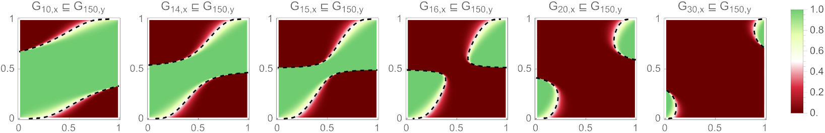
Figure 1: Theorem 1 establishes a sharp threshold around $n^{*}=n^{*}(p_{1},p_{2},N):=2\log_{a}N+1$ for the appearance of the binomial random graph $G_{n,p_{1}}$ as an induced subgraph of the independent random graph $G_{N,p_{2}}$. It also yields the induced containment probability estimate ${\mathbb{P}(G_{n^{*}+c,p_{1}}\sqsubseteq G_{N,p_{2}})\approx f_{p_{1},p_{2}}(c)}$, which allows us to reproduce an idealized version of Figure 5 in [15], where $\mathbb{P}(G_{n,x}\sqsubseteq G_{N,y})$ with $N=150$ is empirically plotted for all $x,y\in[0,1]$ and ${n\in\{10,14,15,16,20,30\}}$; the dashed line corresponds to the threshold $n^{*}$. Previous work [4] applied to the special case $p_{1}=p_{2}=1/2$, i.e., only reproduced the central point in each plot.

Our first result establishes a sharp threshold for the appearance of the binomial random graph $G_{n,p_{1}}$ as an induced subgraph of the independent random graph $G_{N,p_{2}}$, resolving an open problem of Chatterjee and Diaconis [4]. Below the abbreviation $F\sqsubseteq G$ means that $G$ contains an induced copy of $F$.

Theorem 1 (Sharp threshold).

Let $p_{1},p_{2}\in(0,1)$ be constants. Define $a:={1/\bigl{(}p_{2}^{p_{1}}(1-p_{2})^{1-p_{1}}\bigr{)}}$ and ${\varepsilon_{N}:=(\log\log N)^{2}/\log N}$. Then the following holds, for independent binomial random graphs $G_{n,p_{1}}$ and $G_{N,p_{2}}$:

1. If $p_{2}=1/2$, then

   $$\vspace{-0.25em}\lim_{N\to\infty}\mathbb{P}\bigl{(}G_{n,p_{1}}\sqsubseteq G_{N,p_{2}}\bigr{)} =\begin{cases}1\ \ \ \ &\text{if $n\leq 2\log_{a}N+1-\varepsilon_{N}$,}\\ 0\ \ \ \ &\text{if $n\geq 2\log_{a}N+1+\varepsilon_{N}$.}\end{cases}\hskip 25.00003pt\vspace{-0.25em}$$ (1)

   $$\lim_{N\to\infty}\mathbb{P}\bigl{(}G_{n,p_{1}}\sqsubseteq G_{N,p_{2}}\bigr{)} =\begin{cases}1&\text{if $n-(2\log_{a}N+1)\to-\infty$,}\\ f(c)&\text{if $n-(2\log_{a}N+1)\to c\in(-\infty,+\infty)$,}\\ 0&\text{if $n-(2\log_{a}N+1)\to\infty$,}\end{cases}\hskip 25.00003pt\vspace{-0.125em}$$ (2)

   where $f(c)=f_{p_{1},p_{2}}(c):=\mathbb{P}\bigl{(}\mathrm{N}(0,\sigma^{2})\geq c\bigr{)}$ for a normal random variable $\mathrm{N}(0,\sigma^{2})$ with mean $0$ and variance $\sigma^{2}:=2p_{1}(1-p_{1}){\log^{2}_{a}(1/p_{2}-1)}$.

In concrete words, Theorem 1 shows that, around the threshold $n\approx 2\log_{a}N+1$, the induced containment probability $\mathbb{P}(G_{n,p_{1}}\sqsubseteq G_{N,p_{2}})$ drops from $1-o(1)$ to $o(1)$ in a window of size at most two when ${p_{2}=1/2}$, whereas this window has unbounded size when ${p_{2}\neq 1/2}$. Our proof explains why this new phenomenon happens in the non-uniform case ${p_{2}\neq 1/2}$: here the asymmetry of edges and non-edges makes ${\mathbb{P}(G_{n,p_{1}}\sqsubseteq G_{N,p_{2}}\mid G_{n,p_{1}})}$ strongly dependent on the number of edges in $G_{n,p_{1}}$, which does not occur in the uniform case ${p_{2}=1/2}$ considered in previous work [4]. This edge-deviation effect turns out to be the driving force behind the limiting probability ${f(c)\in(0,1)}$ in (2); see Section 1.3.1 for more proof heuristics.

Theorem 1 confirms the simulation based predictions of McCreesh, Prosser, Solnon and Trimble [16, 15], who empirically plotted the induced containment probability $\mathbb{P}(G_{n,x}\sqsubseteq G_{N,y})$ for $N=150$ and predicted a phase transition near ${n\approx 2\log_{a}N}$; see Figure 5 and Section 3.1 in [15]. Figure 1 illustrates that the fuzziness they found near their predicted threshold can be explained by the limiting probability $f(c)$ in (2), whose existence was not predicted in earlier work (of course, the ‘small number of vertices’ effect also leads to some discrepancies in the plots, in particular for very small and large edge-probabilities in Figure 1).

The classical problems of determining the size of the largest independent set and clique of $G_{N,p_{2}}$ are both related to Theorem 1, as they would correspond to the excluded edge-probabilities ${p_{1}\in\{0,1\}}$. These two classical parameters $\alpha(G_{N,p_{2}})$ and $\omega(G_{N,p_{2}})$ are well-known [2, 13] to typically have size ${2\log_{a}N-\Theta(\log\log N)}$ for $a\in\{1/(1-p_{2}),1/p_{2}\}$, and this additive $\Theta(\log\log N)$ left-shift compared to the threshold from Theorem 1 stems from an important conceptual difference: $n$-vertex cliques and independent sets have an automorphism group of size $n!$, whereas $G_{n,p_{1}}$ typically has a trivial automorphism group. This is one reason why our proof needs to take pseudorandom properties of random graphs into account; see also Sections 1.3.1 and 1.3.3.

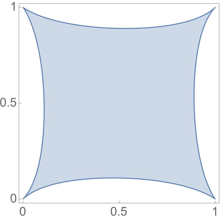
(a)

(b)

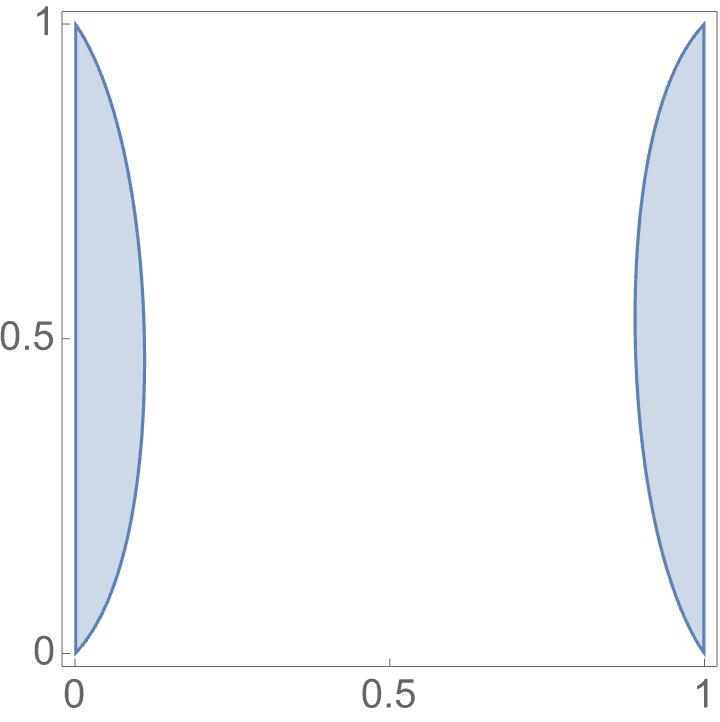
(c)

Figure 2: Theorem 3 establishes two-point concentration around $n_{N}$ of the maximum common induced subgraph of two independent binomial random graphs $G_{N,p_{1}}$ and $G_{N,p_{2}}$. The plots illustrate how the form of $n_{N}$ subdivides the unit square of edge-probabilities ${(p_{1},p_{2})\in(0,1)^{2}}$: we have ${n_{N}=x^{(0)}_{N}(\hat{p})\sim 4\log_{b_{0}(\hat{p})}N}$ in region (a), ${n_{N}\sim x^{(1)}_{N}(p^{*}_{1})\sim 2\log_{b_{1}(p^{*}_{1})}N}$ in region (b), and ${n_{N}\sim x^{(2)}_{N}(p^{*}_{2})\sim 2\log_{b_{2}(p^{*}_{2})}N}$ in region (c), where $\hat{p}$ is defined as in (8) and $p^{*}_{i}$ is the unique solution of $\log b_{0}(p)=2\log b_{i}(p)$; see Lemma 8 in Appendix A. Previous work [4] applied to the special case $p_{1}=p_{2}=1/2$, i.e., only to the central point in region (a).

As a consequence of our proof of Theorem 1, we are able to determine the asymptotic distribution of the number of induced copies of $G_{n,p_{1}}$ in $G_{N,p_{2}}$, resolving another open problem of Chatterjee and Diaconis [4]. In concrete words, Theorem 2 (i) shows that the number of induced copies has a Poisson distribution for ${p_{2}=1/2}$ and $n$ close to the sharp threshold location ${2\log_{a}N+1}$. Furthermore, Theorem 2 LABEL:enum:contain:dist:other shows that the number of induced copies has a ‘squashed’ log-normal distribution for ${p_{2}\neq 1/2}$ and ${n=2\log_{a}N+\Theta(1)}$, which is a rather unusual limiting distribution for random discrete structures (that intuitively arises since the number of such induced copies is so strongly dependent on the number of edges in $G_{n,p_{1}}$; see Section 2.2).

Theorem 2 (Asymptotic distribution).

Let $p_{1},p_{2}\in(0,1)$ be constants. Define $a:={1/\bigl{(}p_{2}^{p_{1}}(1-p_{2})^{1-p_{1}}\bigr{)}}$ and ${\varepsilon_{N}:=(\log\log N)^{2}/\log N}$ as in Theorem 1. For independent binomial random graphs $G_{n,p_{1}}$ and $G_{N,p_{2}}$, let $X=X_{n,N}$ denote the number of induced copies of $G_{n,p_{1}}$ in $G_{N,p_{2}}$. Then the following holds, as $N\to\infty$:

1. If $p_{2}=1/2$ and $2\log_{a}N-1+\varepsilon_{N}\leq n\leq N$, then $X$ has asymptotically Poisson distribution with mean $\mu=\mu_{n,N}:=(N)_{n}2^{-\binom{n}{2}}=\bigl{(}N\cdot 2^{-(n-1)/2+O(n/N)}\bigr{)}^{n}$, i.e.,

   $$\mathrm{d}_{\mathrm{TV}}\bigl{(}X,\>\mathrm{Po}(\mu)\bigr{)}\> \to\>0.$$ (3)

   $$\frac{\log(1+X)}{\log N}\> \overset{\mathrm{d}}{\to}\>\mathrm{SN}\Bigl{(}-c,\;2p_{1}(1-p_{1}){\log^{2}_{a}(1/p_{2}-1)}\Bigr{)},$$ (4)

   where $\mathrm{SN}(\mu,\sigma^{2})$ has cumulative distribution function $F(x):={\mathbbm{1}_{\{{x\geq 0}\}}\mathbb{P}(\mathrm{N}(\mu,\sigma^{2})\leq x)}$.

1.2 Maximum common induced subgraph problem for random graphs

In the maximum common induced subgraph problem the objective is to determine the maximum size of an induced subgraph of $F$ that is isomorphic to an induced subgraph of $G$, where the maximum size is with respect to the number of vertices (this generalizes the induced subgraph isomorphism problem, since the maximum common induced subgraph is $F$ if and only if $F$ is isomorphic to an induced subgraph of $G$). In this paper we focus on this problem for two independent binomial random graphs $F=G_{N,p_{1}}$ and $G=G_{N,p_{2}}$, with constant edge-probabilities $p_{1},p_{2}\in(0,1)$. One motivation here comes from combinatorial probability theory [4], where the following paradox was recently pointed out: two independent infinite random graphs with edge-probabilities $p_{1},p_{2}\in(0,1)$ are isomorphic with probability one, but two independent finite random graphs $G_{N,p_{1}}$ and $G_{N,p_{2}}$ are isomorphic with probability tending to zero as $N\to\infty$. This discontinuity of limits raises the question of finding the size of the maximum common induced subgraph of $G_{N,p_{1}}$ and $G_{N,p_{2}}$, which also is a natural random graph problem in its own right. Chatterjee and Diaconis [4] answered this question in the special case $p_{1}=p_{2}=1/2$. In this paper we resolve the general case with edge-probabilities ${(p_{1},p_{2})\in(0,1)^{2}}$: we discover that the general form of the maximum size is significantly more complicated than for uniform random graphs, which in fact is closely linked to large variance difficulties.

Our next result establishes two-point concentration of the size $I_{N}$ of the maximum common induced subgraph of two independent binomial random graphs $G_{N,p_{1}}$ and $G_{N,p_{2}}$, resolving an open problem of Chatterjee and Diaconis [4]. In concrete words, Theorem 3 shows that $I_{N}$ equals, with probability tending to one as $N\to\infty$, one of (at most) two consecutive integers; see (5)–(6) below.

Theorem 3 (Two-point concentration).

Let $p_{1},p_{2}\in(0,1)$ be constants. For independent binomial random graphs $G_{N,p_{1}}$ and $G_{N,p_{2}}$, define $I_{N}$ as the size of the maximum common induced subgraph. Then

$$\lim_{N\to\infty}\mathbb{P}\bigl{(}I_{N}\in\{\left\lfloor n_{N}-\varepsilon_{N}\right\rfloor,\left\lfloor n_{N}+\varepsilon_{N}\right\rfloor\}\bigr{)}=1,$$ (5)

where $\varepsilon_{N}:=(\log\log N)^{2}/\log N$ and the parameter $n_{N}=n_{N}(p_{1},p_{2})$ defined in Remark 1 satisfies

$$n_{N}=\frac{4\log N+O(\log\log N)}{\min_{p\in[0,1]}\max\bigl{\{}\log b_{0}(p),\>2\log b_{1}(p),\>2\log b_{2}(p)\bigr{\}}},$$ (6)

where, using the convention $0^{0}=1$, we have

$${b_{0}}={b_{0}}(p):=\left(\frac{p}{p_{1}p_{2}}\right)^{p}\left(\frac{1-p}{(1-p_{1})(1-p_{2})}\right)^{1-p}\quad\text{ and }\quad b_{i}=b_{i}(p):=\left(\frac{p}{p_{i}}\right)^{p}\left(\frac{1-p}{1-p_{i}}\right)^{1-p}.$$ (7)

Interestingly, Figure 2 shows that the form of the two-point concentration location $n_{N}=n_{N}(p_{1},p_{2})$ changes as we vary the edge-probabilities $(p_{1},p_{2})\in(0,1)^{2}$, which is a rather surprising phenomenon for random graphs with constant edge-probabilities. In Section 1.3.2 we discuss how the three different forms of $n_{N}$ heuristically arise (due to containment in $G_{N,p_{1}}$, containment in $G_{N,p_{2}}$, and containment in both). The value of $p$ which attains the minimum in (6) is an approximation of the edge-density of a maximum common induced subgraph in $G_{N,p_{1}}$ and $G_{N,p_{2}}$. There is a natural guess for the ‘correct’ edge-density: if we condition on $G_{n,p_{1}}$ and $G_{n,p_{2}}$ being equal, then using linearity of expectation the expected edge-density equals

$$\mathbb{E}\biggl{(}\frac{e\bigl{(}G_{n,p_{1}}\bigr{)}}{\binom{n}{2}}\>\bigg{|}\>G_{n,p_{1}}=G_{n,p_{2}}\biggr{)}=\frac{p_{1}p_{2}}{p_{1}p_{2}+(1-p_{1})(1-p_{2})}=:\hat{p}(p_{1},p_{2})=\hat{p}.$$ (8)

It turns out that $\hat{p}$ is indeed the correct edge-density for a range of edge-probabilities ${(p_{1},p_{2})\in(0,1)^{2}}$; see region (a) in Figure 2. In those cases Corollary 4 gives the two-point concentration location explicitly (the derivation is deferred to Appendix A), which in the special case $p_{1}=p_{2}=1/2$ recovers [4, Theorem 1.1].

Corollary 4 (Special cases).

Let $p_{1},p_{2}\in(0,1)$ be constants satisfying $\log b_{0}(\hat{p})>\max\bigl{\{}2\log b_{1}(\hat{p}),\>2\log b_{2}(\hat{p})\bigr{\}}$ for $b_{j}(p)$ is as defined in (7), which in particular holds when $p_{1}=p_{2}$. For independent binomial random graphs $G_{N,p_{1}}$ and $G_{N,p_{2}}$, define $I_{N}$ as the size of the maximum common induced subgraph. Then

$$\lim_{N\to\infty}\mathbb{P}\bigl{(}I_{N}\in\bigl{\{}\bigl{\lfloor}x^{(0)}_{N}(\hat{p})-\varepsilon_{N}\bigr{\rfloor},\bigl{\lfloor}x^{(0)}_{N}(\hat{p})+\varepsilon_{N}\bigr{\rfloor}\bigr{\}}\bigr{)}=1,$$ (9)

where $\varepsilon_{N}:=(\log\log N)^{2}/\log N$, $\hat{p}=\hat{p}(p_{1},p_{2})$ is defined as in (8), $b_{0}=b_{0}(p)$ is defined as in (7), and

$$x^{(0)}_{N}(p) :=4\log_{b_{0}}N-2\log_{b_{0}}\log_{b_{0}}N-2\log_{b_{0}}(4/e)+1.$$ (10)

In general, the two-point concentration location $n_{N}=n_{N}(p_{1},p_{2})$ is defined in (11) as the solution of an optimization problem over all edge-densities $p\in[0,1]$ of a potential maximum common subgraph. In Section 1.3.2 we discuss how this more complicated form of $n_{N}$ stems from large variance difficulties that can arise in the second moment method arguments (where the typical number of copies can be zero even when the expected number of copies tends to infinity). While the definition (11) of $n_{N}$ involves two implicitly defined (12) parameters $x^{(i)}_{N}(p)$, we remark that when $n_{N}=x^{(i)}_{N}(p)$ holds for $i\in\{1,2\}$, then $x^{(i)}_{N}(p)$ has the explicit form given in (13) below; see Lemma 8 in Appendix A for further estimates of $n_{N}$.

Remark 1 (Explicit expression for $n_{N}$).

The proof of Theorem 3 uses

$$n_{N}=n_{N}(p_{1},p_{2}):=\max_{p\in[0,1]}\;\min\left\{x^{(0)}_{N}(p),\>x^{(1)}_{N}(p),\>x^{(2)}_{N}(p)\right\},$$ (11)

where $x^{(0)}_{N}(p)$ is as defined in (10), and $x^{(i)}_{N}=x^{(i)}_{N}(p)$ with $i\in\{1,2\}$ is the unique solution to

$$e\cdot N\;=\;x^{(i)}_{N}(p)\cdot b_{i}^{\bigl{(}x^{(i)}_{N}(p)-1\bigr{)}/2},$$ (12)

where $b_{i}=b_{i}(p)$ is as defined in (7). Furthermore, if $n_{N}=x^{(i)}_{N}(p)$ holds in (11) for $i\in\{1,2\}$, then

$$x^{(i)}_{N}(p) =2\log_{b_{i}}N-2\log_{b_{i}}\log_{b_{i}}N-2\log_{b_{i}}(2/e)+1+O\left(\frac{\log\log N}{\log N}\right).$$ (13)

1.3 Intuition and proof heuristics

The proofs of our main results are based on involved applications of the first and second moment method, which each require an extra twist due to large variance (that prevents standard applications of these methods). In the following we highlight some of the key intuition and heuristics going into our arguments.

1.3.1 Induced subgraph isomorphism problem

We now heuristically discuss the sharp threshold for induced containment ${G_{n,p_{1}}\sqsubseteq G_{N,p_{2}}}$. Besides outlining the reasoning behind our proof approach for Theorem 1, we also motivate why the threshold is located around ${n\approx 2\log_{a}N+1}$, and clarify why the case ${p=1/2}$ behaves so differently than the case ${p\neq 1/2}$.

The natural proof approach would be to apply the first and second moment method to the random variable $X$ that counts the number of induced copies of $G_{n,p_{1}}$ in $G_{N,p_{2}}$. While this approach can indeed be used to establish (1) when ${p_{2}=1/2}$ (as done in [4] for $p_{1}=p_{2}=1/2$), it fails when ${p_{2}\neq 1/2}$: the reason is $\operatorname{Var}X\gg(\mathbb{E}X)^{2}$, i.e., that the variance of $X$ is too large to apply the second moment method.

We overcome this second moment challenge for $p_{2}\neq 1/2$ by identifying the key reason for the large variance, which turns out to be random fluctuations of the number of edges in $G_{n,p_{1}}$. To work around the effect of these edge-fluctuations we use a multi-round exposure approach, where we first reveal $G_{n,p_{1}}$ and then $G_{N,p_{2}}$ (which conveniently allows us to deal with one source of randomness at a time). When we reveal $G_{n,p_{1}}$, we exploit that $H:=G_{n,p_{1}}$ will typically be asymmetric and satisfy other pseudorandom properties. Writing $X_{H}$ for the number of induced copies of $H$ in $G_{N,p_{2}}$, we then focus on the conditional probability

$$\operatorname{\mathbb{P}}(G_{n,p_{1}}\sqsubseteq G_{N,p_{2}}\mid G_{n,p_{1}}=H)=\mathbb{P}(H\sqsubseteq G_{N,p_{2}})=\operatorname{\mathbb{P}}(X_{H}\geq 1).$$ (14)

To see how the number of edges in $H$ affects this containment probability, suppose for concreteness that $H$ has $m=\binom{n}{2}p_{1}+\delta n/2$ edges. Recalling $a={1/\bigl{(}p_{2}^{p_{1}}(1-p_{2})^{1-p_{1}}\bigr{)}}$, it turns out (see (31)–(32) in Section 2.1 for the routine details) that the expected number of induced copies of $H$ in $G_{N,p_{2}}$ satisfies

$$\mathbb{E}X_{H}=(N)_{n}\cdot p_{2}^{m}(1-p_{2})^{\binom{n}{2}-m}=\biggl{[}\left(\frac{p_{2}}{1-p_{2}}\right)^{\delta/2}Ne^{-\log a\cdot(n-1)/2+O(n/N)}\biggr{]}^{n}.$$ (15)

For $n=2\log_{a}N+1+c$ and $p_{2}\neq 1/2$ it follows from (15) that the value of the edge-deviation parameter $\delta$ determines whether $\mathbb{E}X_{H}$ goes to $\infty$ or $0$, i.e., depending on whether ${\delta\log\bigl{(}p_{2}/(1-p_{2})\bigr{)}}$ is smaller or larger than ${c\log a}$ (here we also see why the case $p_{2}=1/2$ behaves so differently: in (15) the term involving $\delta$ equals one and thus disappears). With some technical effort, we can make the first moment heuristic that $\mathbb{E}X_{H}\to\infty$ implies $\operatorname{\mathbb{P}}(X_{H}\geq 1)\to 1$ rigorous, i.e., use the first and second moment method to show that

$$\operatorname{\mathbb{P}}(X_{H}\geq 1)=\begin{cases}o(1)\quad&\text{if~{}$\delta\log\bigl{(}p_{2}/(1-p_{2})\bigr{)}<c\log a$,}\\ 1-o(1)\quad&\text{if~{}$\delta\log\bigl{(}p_{2}/(1-p_{2})\bigr{)}>c\log a$,}\end{cases}$$ (16)

where a good control of the ‘overlaps’ of different $H$ in the variance calculations requires us to identify and exploit suitable pseudorandom properties of $H$ (which we can ‘with foresight’ insert into our argument when we first reveal ${H=G_{n,p_{1}}}$). The crux is that the containment conditions in (16) only depend on deviations in the number $e(G_{n,p_{1}})={\binom{n}{2}p_{1}+\delta n/2}$ of edges in $G_{n,p_{1}}$, which in view of (14) intuitively translates into

$$\operatorname{\mathbb{P}}(G_{n,p_{1}}\sqsubseteq G_{N,p_{2}})=\mathbb{P}\biggl{(}\frac{e(G_{n,p_{1}})-\tbinom{n}{2}p_{1}}{n/2}\cdot\log\bigl{(}p_{2}/(1-p_{2})\bigr{)}>c\log a\biggr{)}+o(1)$$ (17)

for $n=2\log_{a}N+1+c$. This in turn makes the threshold result (2) plausible via the Central Limit Theorem (in fact, (17) is also consistent with the form of (1) for $p_{2}=1/2$, since then ${\log\bigl{(}p_{2}/(1-p_{2})\bigr{)}=0}$); see Section 2.1 for the full technical details of the proof of Theorem 1.

With this knowledge about $X_{H}$ in hand, the distributional result Theorem 2 follows without much extra conceptual work. Indeed, for $p\neq 1/2$ we obtain the unusual limiting distribution (4) by exploiting that the event $X_{H}\geq 1$ in the second moment method based $1-o(1)$ statement in (16) can be strengthened to $X_{H}\approx\mathbb{E}X_{H}$; see Section 2.2. Furthermore, for $p=1/2$ we obtain the Poisson limiting distribution (3) by refining our variance estimates in order to apply the Stein-Chen method to $X_{H}$; see Section 2.3.

1.3.2 Maximum common induced subgraph problem

We now heuristically discuss the two-point concentration of the size $I_{N}$ of the maximum common induced subgraph in $G_{N,p_{1}}$ and $G_{N,p_{2}}$. Our main focus is on motivating the ‘correct’ typical value $I_{N}\approx n_{N}$ in Theorem 3, which requires a refinement of the vanilla first and second moment approach. For ease of exposition, here we shall restrict our attention to the first-order asymptotics of $n_{N}=n_{N}(p_{1},p_{2})$ from (6).

Armed with the first and second moment insights for $X_{H}$ from the heuristic discussion in Section 1.3.1, the natural approach towards determining the typical value of $I_{N}$ would be to focus on the random variables $X_{n,m}:=\sum_{H\in\mathcal{G}_{n,m}}X^{(1)}_{H}X^{(2)}_{H}$, where $\mathcal{G}_{n,m}$ denotes the set of all unlabeled graphs with $n$ vertices and $m$ edges, and $X^{(i)}_{H}$ counts the number of induced copies of $H$ in $G_{N,p_{i}}$. Here the crux is that

$$I_{N}=\max\bigl{\{}n\>:\>\text{$X_{n,m}\geq 1$ for some~{}$0\leq m\leq\tbinom{n}{2}$}\bigr{\}}.$$ (18)

Using $|\mathcal{G}_{n,m}|=\binom{\binom{n}{2}}{m}e^{O(n\log n)}$ and the independence of $G_{N,p_{1}}$ and $G_{N,p_{2}}$, similar to (15) it turns out (see (60) and (68) in Section 3.1 for the details) that for edge-density $p=p(m,n):=m/\binom{n}{2}$ we have

$$\begin{split}\mathbb{E}X_{n,m}&=e^{O(n\log n)}\binom{\binom{n}{2}}{m}\prod_{i\in\{1,2\}}(N)_{n}p_{i}^{m}(1-p_{i})^{\binom{n}{2}-m}=\left[N^{2}e^{-\frac{n}{2}\log{b_{0}}(p)+O(\log n)}\right]^{n}.\end{split}$$ (19)

Taking into account when these expectations go to $0$ and $\infty$, in view of (18) and standard first moment heuristics it then is natural to guess that the typical value of $I_{N}$ should be approximately

$$n_{N}\approx\max_{p\in[0,1]}4\log_{b_{0}(p)}N=\frac{4\log N}{\min_{p\in[0,1]}\log b_{0}(p)}=4\log_{b_{0}(\hat{p})}N,$$ (20)

where $\hat{p}=\hat{p}(p_{1},p_{2})$ from (8) turns out to be the unique minimizer of $\log b_{0}(p)$ from (7). For this choice of $n_{N}$ it turns out that we indeed typically have ${I_{N}\approx n_{N}}$ for a range of edge-probabilities ${(p_{1},p_{2})\in(0,1)^{2}}$, including the special case $p_{1}=p_{2}$; see Corollary 4 and region (a) in Figure 2.

For general edge-probabilities ${(p_{1},p_{2})\in(0,1)^{2}}$ the ‘correct’ form of $n_{N}$ is more complicated than our first guess (20), and the key reason turns out to be that due to large variance we can have ${\mathbb{P}(X_{n,m}\geq 1)\to 0}$ despite ${\mathbb{E}X_{n,m}\to\infty}$. We overcome this difficulty by realizing that containment in $G_{N,p_{i}}$ can, from a ‘first moment perspective’, sometimes be harder than containment in both $G_{N,p_{1}}$ and $G_{N,p_{2}}$, i.e., that we can have ${\mathbb{E}X^{(i)}_{n,m}\to 0}$ for $X^{(i)}_{n,m}:=\sum_{H\in\mathcal{G}_{n,m}}X^{(i)}_{H}$ despite ${\mathbb{E}X_{n,m}\to\infty}$. Similarly to (19) and (15) it turns out (see (58) in Section 3.1 for the details) that for edge-density $p=p(m,n)=m/\binom{n}{2}$ we have

$$\begin{split}\mathbb{E}X^{(i)}_{n,m}&=e^{O(n\log n)}\binom{\binom{n}{2}}{m}\cdot(N)_{n}p_{i}^{m}(1-p_{i})^{\binom{n}{2}-m}=\left[Ne^{-\frac{n}{2}\log{b_{i}}(p)+O(\log n)}\right]^{n}.\end{split}$$ (21)

Note that $X_{n,m}\geq 1$ implies both $X^{(1)}_{n,m}\geq 1$ and $X^{(2)}_{n,m}\geq 1$. Taking into account when the two expectations in (21) go to $0$, we thus refine our first guess (20) for the typical value of $I_{N}$ to approximately

$$\begin{split}n_{N}&\approx\max_{p\in[0,1]}\min\bigl{\{}4\log_{b_{0}(p)}N,\>2\log_{b_{1}(p)}N,\>2\log_{b_{2}(p)}N\bigr{\}}\\ &=\frac{4\log N}{\min_{p\in[0,1]}\max\bigl{\{}\log b_{0}(p),\>2\log b_{1}(p),\>2\log b_{2}(p)\bigr{\}}}.\end{split}$$ (22)

This turns out to be the ‘correct’ value of $n_{N}$ up to second order correction terms, see (6) and Figure 2. Indeed, with substantial technical effort (more involved than for the induced subgraph isomorphism problem) we can use refinements of the first and second moment method to prove two-point concentration of form ${I_{N}\approx n_{N}}$ for all edge-probabilities ${(p_{1},p_{2})\in(0,1)^{2}}$; see Section 3 for the full technical details of the proof of Theorem 3.

1.3.3 Pseudorandom properties of random graphs

To enable the technical variance estimates in the proofs of our main results, we need to get good control over the ‘overlaps’ of different induced copies. To this end it will be important to take the pseudorandom properties of random graphs into account, by restricting our attention to graphs $H$ from the following three classes:

• The set of all $n$-vertex graphs $H$ where, for all vertex-subsets ${L\subseteq[n]}$ of size ${|L|\geq n-n^{2/3}}$, the induced subgraph $H[L]$ is asymmetric, i.e., satisfies $|\mathrm{Aut}(H[L])|=1$.

• The set of all $n$-vertex graphs $H$ where, for all non-empty vertex-subsets ${L\subseteq[n]}$, the induced subgraph $H[L]$ contains $e(H[L])=\tbinom{|L|}{2}m/\tbinom{n}{2}\pm n^{2/3}(n-|L|)$ edges.

• The set of all $n$-vertex graphs $H$ with $e(H)=\tbinom{n}{2}p\pm n^{4/3}$ edges.

In concrete words, the first property $\mathcal{A}_{n}$ formalizes the folklore fact that all very large subsets of random graphs are asymmetric; see [2, 9, 14]. The second and third properties $\mathcal{E}_{n,m}$ and $\mathcal{F}_{n,p}$ formalize the well-known fact that the edges of a random graph are well-distributed; see [1, 2, 10]. The following auxiliary lemma states that these are indeed typical properties of dense random graphs (we defer the proof to Appendix B, since it is rather tangential to our main arguments). Below $G_{n,m}$ denotes the uniform random graph, which is chosen uniformly at random from all $n$-vertex graphs with exactly $m$ edges. Furthermore, the abbreviation whp (with high probability) means with probability tending to one as the number of vertices goes to infinity.

Lemma 5 (Random graphs are pseudorandom).

Let $p,\gamma\in(0,1)$ be constants. Then the following holds:

1. For all $\gamma\tbinom{n}{2}\leq m\leq(1-\gamma)\tbinom{n}{2}$, the uniform random graph whp satisfies $G_{n,m}\in\mathcal{A}_{n}\cap\mathcal{E}_{n,m}$.

2. The binomial random graph whp satisfies $G_{n,p}\in\mathcal{A}_{n}\cap\mathcal{F}_{n,p}$.

The reason for why we only consider the edge-property $\mathcal{E}_{n,m}$ for the uniform random graph $G_{n,m}$ is conceptual: the edges of $G_{n,m}$ are simply more well-distributed than the edges of the binomial random $G_{n,p}$ with $p:=m/\binom{n}{2}\in[\gamma,1-\gamma]$, where for large vertex-subsets $L\subseteq[n]$ of size $|L|=n-o(n^{1/3})$ we expect that typically $\bigl{|}e(G_{n,p}[L])-\tbinom{|L}{2}p\bigr{|}=\Omega\bigl{(}|L|\sqrt{p(1-p)}\bigr{)}\gg n^{2/3}(n-|L|)$ holds.

2 Induced subgraph isomorphism problem

This section is devoted to the induced subgraph isomorphism problem for two independent random graphs $G_{n,p_{1}}$ and $G_{N,p_{2}}$ with constant edge-probabilities ${p_{1},p_{2}\in(0,1)}$. It naturally splits into several parts: in the core Section 2.1 we prove the sharp threshold result Theorem 1, and in the subsequent Sections 2.2–2.3 we then separately prove the two parts of the distributional result Theorem 2.

2.1 Sharp Threshold: Proof of Theorem 1

In this section we prove Theorem 1, i.e., establish a sharp threshold for the appearance of an induced copy of $G_{n,p_{1}}$ in $G_{N,p_{2}}$, where $p_{1},p_{2}\in(0,1)$. Our proof-strategy is somewhat roundabout, since we need to deal with the difficulty that for $p_{2}\neq 1/2$ the induced containment event $G_{n,p_{1}}\sqsubseteq G_{N,p_{2}}$ is sensitive towards small variations in the number of edges of $G_{n,p_{1}}$ (as discussed in Sections 1.1 and 1.3.1). For this reason we first prove a sharp threshold result for the event that $G_{N,p_{2}}$ contains an induced copy of a particular $n$-vertex pseudorandom graph $H$ with $m$ edges (see Lemma 6 below). Since $G_{n,p_{1}}$ will typically be pseudorandom by Lemma 5, this then effectively reduces the problem of estimating ${\mathbb{P}(G_{n,p_{1}}\sqsubseteq G_{N,p_{2}})}$ to understanding deviations in the number of edges of $G_{n,p_{1}}$, which is a well-understood and much simpler problem.

Turning to the details, to restrict our attention to graphs with pseudorandom properties we introduce

$$\mathcal{T}_{n,m}:=\mathcal{A}_{n}\cap\mathcal{E}_{n,m},$$ (23)

where the asymmetry property $\mathcal{A}_{n}$ and the edge-distribution property $\mathcal{E}_{n,m}$ are defined as in Section 1.3.3. For edge-counts $m$ of interest, Lemma 5 shows that the uniform random graph whp satisfies $G_{n,m}\in\mathcal{T}_{n,m}$, so Lemma 6 effectively gives a sharp threshold result for the induced containment $G_{n,m}\sqsubseteq G_{N,p_{2}}$.

Lemma 6 (Sharp threshold for pseudorandom graphs).

Let $p_{1},p_{2}\in(0,1)$ be constants. Define $a:={1/(p_{2}^{p_{1}}(1-p_{2})^{1-p_{1}})}$, $\varepsilon_{N}:={(\log\log N)^{2}/\log N}$, and $\psi:={\log_{a}\bigl{(}p_{2}/(1-p_{2})\bigr{)}}$. If $\delta_{m}:={\bigl{[}m-\tbinom{n}{2}p_{1}\bigr{]}/(n/2)}$ and $c_{N}:={n-(2\log_{a}N+1)}$ satisfy ${\left|\psi\delta_{m}\right|=o(n)}$ and ${\left|c_{N}\right|=o(\log_{a}N)}$, then the following holds: as $N\to\infty$, for any graph $H\in\mathcal{T}_{n,m}$:

$$\mathbb{P}\bigl{(}H\sqsubseteq G_{N,p_{2}}\bigr{)}=\begin{cases}o(1)\quad&\text{if~{}$\psi\delta_{m}-c_{N}\leq-\varepsilon_{N}$,}\\ 1-o(1)\quad&\text{if~{}$\psi\delta_{m}-c_{N}\geq\varepsilon_{N}$.}\end{cases}$$ (24)

Remark 2.

The $o(1)$ statement in (24) remains valid for any $n$-vertex graph $H$ with $e(H)=m$ edges.

Before giving the (first and second moment based) proof of Lemma 6, we first show how it implies Theorem 1 using a multi-round exposure argument, where we first reveal the number of edges of $G_{n,p_{1}}$, then reveal the random graph $G_{n,p_{1}}$, and afterwards try to embed $G_{n,p_{1}}$ into the random graph $G_{N,p_{2}}$, each time discarding atypical outcomes along the way (so that we can focus on pseudorandom $G_{n,p_{1}}$).

Proof of Theorem 1.

To estimate the probability that $G_{n,p_{1}}\sqsubseteq G_{N,p_{2}}$ holds, by monotonicity in $n$ it suffices to consider the case where $c_{N}=o(\log\log N)$ holds (in fact $c_{N}=O(1)$ suffices, since $\lim_{c\to\infty}f(c)=0$ and $\lim_{c\to-\infty}f(c)=1$ when $p_{2}\neq 1/2$). Since $G_{n,p_{1}}$ conditioned on having $m$ edges has the same distribution as $G_{n,m}$, by using Lemma 5 to handle outcomes of $G_{n,p_{1}}$ with an atypical number of edges $e(G_{n,p_{1}})$ it follows that

$$\begin{split}\Bigl{|}\mathbb{P}(G_{n,p_{1}}\sqsubseteq G_{N,p_{2}})-\!\sum_{m:\bigl{|}m-\tbinom{n}{2}p_{1}\bigr{|}\leq n^{4/3}}\!\!\!\!\!\!\!\!\!\!\!\!\mathbb{P}(G_{n,m}\sqsubseteq G_{N,p_{2}})\mathbb{P}(e(G_{n,p_{1}})=m)\Bigr{|}\>\leq\>\mathbb{P}(G_{n,p_{1}}\not\in\mathcal{F}_{n,p_{1}})=o(1).\end{split}$$ (25)

If $\bigl{|}m-\tbinom{n}{2}p_{1}\bigr{|}\leq n^{4/3}$, then by using Lemma 5 to handle the atypical event $G_{n,m}\not\in\mathcal{T}_{n,m}$ it follows that

$$\begin{split}\Bigl{|}\mathbb{P}(G_{n,m}\sqsubseteq G_{N,p_{2}})-\sum_{H\in\mathcal{T}_{n,m}}\mathbb{P}(H\sqsubseteq G_{N,p_{2}})\mathbb{P}(G_{n,m}=H)\Bigr{|}\>\leq\>\mathbb{P}(G_{n,m}\not\in\mathcal{T}_{n,m})=o(1).\end{split}$$ (26)

In particular, using the sharp threshold result Lemma 6 for the event $H\sqsubseteq G_{N,p_{2}}$ (which applies since $|\psi\delta_{m}|=o(n)$ holds) and Lemma 5 for the typical event $G_{n,m}\in\mathcal{T}_{n,m}$, it follows that (26) implies

$$\mathbb{P}(G_{n,m}\sqsubseteq G_{N,p_{2}})=\begin{cases}o(1)\quad&\text{if~{}$\psi\delta_{m}-c_{N}\leq-\varepsilon_{N}$,}\\ 1-o(1)\quad&\text{if~{}$\psi\delta_{m}-c_{N}\geq\varepsilon_{N}$.}\end{cases}$$ (27)

If $p_{2}=1/2$, then in the setting of (1) we have $\psi=0$ and $\left|c_{N}\right|\geq\varepsilon_{N}$, so the sharp threshold result (1) follows by first inserting estimate (27) into (25) and finally using Lemma 5 to infer $\mathbb{P}(G_{n,p_{1}}\in\mathcal{F}_{n,p_{1}})=1-o(1)$.

We focus on the case $p_{2}\neq 1/2$ in the remainder of the proof. Note that estimate (27) does not apply when $|\psi\delta_{m}-c_{N}|<\varepsilon_{N}$, but we shall now argue that we can effectively ignore this small range of edge-counts $m$ in (25) above. Recall that $n\to\infty$ as $N\to\infty$. By the Central Limit Theorem it thus follows that, as $N\to\infty$,

$$Z:=\psi\delta_{e(G_{n,p_{1}})}=\psi\cdot\frac{e(G_{n,p_{1}})-\tbinom{n}{2}p_{1}}{n/2}\>\overset{\mathrm{d}}{\to}\>\mathrm{N}\bigl{(}0,\;2p_{1}(1-p_{1})\psi^{2}\bigr{)}.$$ (28)

Recalling that $\varepsilon_{N}=o(1)$ and $0<\operatorname{Var}Z=2p_{1}(1-p_{1})\psi^{2}=\Theta(1)$, it follows that

$$\mathbb{P}(|Z-c_{N}|<\varepsilon_{N})\>=\>o(1).$$ (29)

(This alternatively follows from $\max_{k}\mathbb{P}(e(G_{n,p_{1}})=k)\leq O(1)/\sqrt{n^{2}p_{1}(1-p_{1})}\leq O(1/n)$, say.) Inserting estimates (27) and (29) into (25), using Lemma 5 to infer $\mathbb{P}(G_{n,p_{1}}\in\mathcal{F}_{n,p_{1}})=1-o(1)$ it follows that

$$\bigl{|}\mathbb{P}(G_{n,p_{1}}\sqsubseteq G_{N,p_{2}})-\mathbb{P}(Z-c_{N}\geq 0)\bigr{|}\>=\>o(1),$$ (30)

which together with the convergence result (28) and ${\varepsilon_{N}=o(1)}$ establishes the threshold result (2). ∎

In the following proof of Lemma 6 we shall apply the first and second moment method to the random variable $X_{H}$, which we define as the number of induced copies of $H$ in $G_{N,p_{2}}$. Here the restriction to pseudorandom graphs $H\in\mathcal{T}_{n,m}$ will be key for controlling the expectation $\mathbb{E}X_{H}$ and variance $\operatorname{Var}X_{H}$.

Proof of Lemma 6.

Let $H$ be any $n$-vertex graph with $e(H)=m$ edges. Note that ${X_{H}=\sum_{S\in\binom{[N]}{n}}I_{S}}$, where $I_{S}$ is the indicator random variable for the event that the induced subgraph $G_{N,p_{2}}[S]$ is isomorphic to $H$. Note that there are exactly $n!/\left|\mathrm{Aut}(H)\right|$ distinct embeddings of $H$ into $S$. Using linearity of expectation and the standard shorthand $(N)_{n}:=N!/(N-n)!$, in view of $m=\tbinom{n}{2}p_{1}+\delta_{m}n/2$, $a={1/(p_{2}^{p_{1}}(1-p_{2})^{1-p_{1}})}$, $p_{2}/(1-p_{2})=a^{\psi}$ and $(n-1)/2=\log_{a}N+c_{N}/2$ it follows that the expected number of induced copies of $H$ in $G_{N,p_{2}}$ satisfies

$$\begin{split}\mathbb{E}X_{H}&=\sum_{S\in\binom{[N]}{n}}\mathbb{E}I_{S}=\binom{N}{n}\cdot\frac{n!}{\left|\mathrm{Aut}(H)\right|}\cdot p_{2}^{e(H)}(1-p_{2})^{\binom{n}{2}-e(H)}\\ &=\frac{1}{\left|\mathrm{Aut}(H)\right|}\cdot(N)_{n}\cdot p_{2}^{m}(1-p_{2})^{\binom{n}{2}-m}\\ &=\frac{1}{\left|\mathrm{Aut}(H)\right|}\cdot\left[Ne^{O(n/N)}\cdot\left(\frac{p_{2}}{1-p_{2}}\right)^{\delta_{m}/2}a^{-(n-1)/2}\right]^{n}\\ &=\frac{1}{\left|\mathrm{Aut}(H)\right|}\cdot\left[a^{\psi\delta_{m}-c_{N}+o(\varepsilon_{N})}\right]^{n/2},\end{split}$$ (31)

where we used $n/N=\Theta((\log N)/N)=o(\varepsilon_{N})$ and $1<a=O(1)$ for the last step. If ${\psi\delta_{m}-c_{N}\leq-\varepsilon_{N}}$, then using ${|\mathrm{Aut}(H)|\geq 1}$ and Markov’s inequality together with ${\varepsilon_{N}n\to\infty}$ as ${N\to\infty}$, we see that

$$\mathbb{P}(X_{H}>0)\leq\mathbb{E}X_{H}\leq a^{-\Omega(\varepsilon_{N}n)}=o(1),$$

establishing the $o(1)$ statement in (24).

In the remainder we focus on the $1-o(1)$ statement in (24), i.e., we henceforth fix ${H\in\mathcal{T}_{n,m}}$ and assume that ${\psi\delta_{m}-c_{N}\geq\varepsilon_{N}}$. Since ${H\in\mathcal{T}_{n,m}\subseteq\mathcal{A}_{N}}$ implies $\left|\mathrm{Aut}(H)\right|=1$, using estimate (31) we infer that

$$\mu:=\mathbb{E}X_{H}=(N)_{n}\cdot p_{2}^{m}(1-p_{2})^{\binom{n}{2}-m}=\left[a^{\psi\delta_{m}-c_{N}+o(\varepsilon_{N})}\right]^{n/2}\geq a^{\Omega(\varepsilon_{N}n)}\to\infty.$$ (32)

To complete the proof of (24), using Chebyshev’s inequality it thus suffices to show that ${\operatorname{Var}X_{H}=o\bigl{(}(\mathbb{E}X_{H})^{2}\bigr{)}}$. Recall that ${X_{H}=\sum_{S\in\binom{[N]}{n}}I_{S}}$, where $I_{S}$ is the indicator random variable for the event that the induced subgraph $G_{N,p_{2}}[S]$ is isomorphic to $H$. Since $I_{R}$ and $I_{S}$ are independent when ${|R\cap S|\leq 1}$, we have

$$\operatorname{Var}X_{H}\>\leq\>\sum_{2\leq\ell\leq n}\underbrace{\sum_{R,S\in\binom{[N]}{n}:\left|R\cap S\right|=\ell}\mathbb{E}(I_{R}I_{S})}_{=:w_{\ell}}\>=\>\sum_{2\leq\ell<n}w_{\ell}+\underbrace{\mathbb{E}X_{H}}_{=\mu}.$$ (33)

To bound the parameter $w_{\ell}$ defined in (33) for $2\leq\ell<n$, we first note that there are $\binom{N}{n}\binom{n}{\ell}\binom{N-n}{n-\ell}$ ways of choosing $R,S\in\binom{[N]}{n}$ with $|R\cap S|=\ell$. To then get a handle on $\mathbb{E}(I_{R}I_{S})$, we count the number of ways we can embed two induced copies of $H$ into $R\cup S$ so that $G_{N,p_{2}}[R]$ and $G_{N,p_{2}}[S]$ are both isomorphic to $H$: there are $n!$ ways of embedding an induced copy of $H$ into $R$, at most $\binom{n}{n-\ell}\cdot(n-\ell)!=(n)_{n-\ell}$ ways of choosing and embedding $n-\ell$ vertices of a second induced copy of $H$ into $S\setminus R$, and at most $\max_{H\in\mathcal{T}_{n,m},|L|=\ell}|\mathrm{Aut}(H[L])|$ ways of embedding the remaining $\ell$ vertices of the second induced copy of $H$ into $R\cap S$, where the maximum is taken over all vertex-subsets $L\subseteq V(H)$ of size $|L|=\ell$. As these embeddings determine all edges and non-edges in $G_{N,p_{2}}[R\cup S]$, it follows that

$$\begin{split}w_{\ell}\leq\binom{N}{n}\binom{n}{\ell}&\binom{N-n}{n-\ell}\cdot n!\cdot(n)_{n-\ell}\cdot\max_{H\in\mathcal{T}_{n,m},\>\left|L\right|=\ell}|\mathrm{Aut}(H[L])|\\ &\cdot\max_{H\in\mathcal{T}_{n,m},\>\left|L\right|=\ell}p_{2}^{2m-e(H[L])}(1-p_{2})^{2\binom{n}{2}-\binom{\ell}{2}-2m+e(H[L])},\end{split}$$ (34)

where the two maxima in (34) are each taken over all vertex-subsets $L\subseteq V(H)$ of size $|L|=\ell$, as above. Note that ${n=(2+o(1))\log_{a}N}$, which implies $N-n>n-\ell$ for all sufficiently large $N$. Recalling that $\mu=(N)_{n}p_{2}^{m}(1-p_{2})^{\binom{n}{2}-m}$ by (32), using $n^{2}/N=o(1)$ it follows that

$$\frac{w_{\ell}}{\mu^{2}}\leq\underbrace{\frac{(N-n)_{n-\ell}}{(N)_{n}}}_{=(1+o(1))N^{-\ell}}\cdot\binom{n}{\ell}^{2}\cdot\max_{H\in\mathcal{T}_{n,m},\>\left|L\right|=\ell}\left|\mathrm{Aut}(H[L])\right|\cdot\underbrace{\max_{H\in\mathcal{T}_{n,m},\>\left|L\right|=\ell}\biggl{(}\frac{1-p_{2}}{p_{2}}\biggr{)}^{e(H[L])}(1-p_{2})^{-\binom{\ell}{2}}}_{=:P_{\ell}}.$$ (35)

Setting $\zeta:=1/\max\bigl{\{}-2\log_{a}(1-p_{2}),-2\log_{a}(p_{2}),2\bigr{\}}>0$, we now bound $w_{\ell}/\mu^{2}$ further using a case distinction.

Case $2\leq\ell\leq\zeta n$: Here we use $0\leq e(H[L])\leq\binom{\ell}{2}$ to deduce that the parameter $P_{\ell}$ from (35) satisfies

$$P_{\ell}\leq\max_{0\leq k\leq\binom{\ell}{2}}p_{2}^{-k}(1-p_{2})^{-\binom{\ell}{2}+k}\leq\biggl{[}\max\biggl{\{}\frac{1}{p_{2}},\frac{1}{1-p_{2}}\biggr{\}}\biggr{]}^{\binom{\ell}{2}}.$$ (36)

Inserting this estimate and the trivial bound $|\mathrm{Aut}(H[L])|\leq|L|!$ into (35), using $\tbinom{n}{\ell}\leq n^{\ell}/\ell!$ together with $n=(2+o(1))\log_{a}N$ and $\ell\leq\zeta n\leq(1+o(1))\log_{\max\{1/p_{2},1/(1-p_{2})\}}N$, it follows for all large enough $N$ that

$$\begin{split}\frac{w_{\ell}}{\mu^{2}}&\leq 2N^{-\ell}\cdot\binom{n}{\ell}^{2}\ell!\cdot P_{\ell}\leq\Biggl{[}N^{-1}n^{2}\cdot\biggl{[}\max\biggl{\{}\frac{1}{p_{2}},\frac{1}{1-p_{2}}\biggr{\}}\biggr{]}^{(\ell-1)/2}\Biggr{]}^{\ell}\leq N^{-\ell/3}\leq a^{-\Omega(n)}.\end{split}$$ (37)

Case $\zeta n\leq\ell<n$: Here we improve the estimate (36) for $P_{\ell}$ using that $H\in{\mathcal{T}_{n,m}\subseteq\mathcal{E}_{n,m}}$: this pseudorandom edge-property implies that, for any vertex-subset $L\subseteq[n]$ of size $|L|=\ell$, the induced number of edges satisfies $e(H[L])=\tbinom{\ell}{2}m/\tbinom{n}{2}+O(n^{2/3}(n-\ell))$. Recalling $a={1/(p_{2}^{p_{1}}(1-p_{2})^{1-p_{1}})}$, using $m/\tbinom{n}{2}=p_{1}+\delta_{m}/n+O(1/n^{2})$ and $(1-p_{2})/p_{2}=a^{-\psi}$ it follows that the parameter $P_{\ell}$ from (35) satisfies

$$P_{\ell}=a^{\binom{\ell}{2}}\cdot\biggl{(}\frac{1-p_{2}}{p_{2}}\biggr{)}^{\binom{\ell}{2}\delta_{m}/n+O(n^{2/3}(n-\ell))}=a^{(1-\psi\delta_{m}/n)\binom{\ell}{2}+O(\psi n^{2/3}(n-\ell))}.$$ (38)

For $\zeta n\leq\ell<n-n^{2/3}$ we then estimate $|\mathrm{Aut}(H[L])|\leq\ell!\leq n^{\ell}\leq e^{O(n^{2/3}(n-\ell))}$, and for $n-n^{2/3}\leq\ell<n$ we use ${H\in\mathcal{T}_{n,m}\subseteq\mathcal{A}_{n}}$ to obtain $\max_{|L|=\ell}|\mathrm{Aut}(H[L])|=1$. Note that $1<a=O(1)$ and $\psi=O(1)$. We now insert these estimates and ${\tbinom{n}{\ell}=\tbinom{n}{n-\ell}\leq n^{n-\ell}}$ into (35). Then, using $\ell-1=(n-1)-(n-\ell)$ and $\left|\psi\delta_{m}/n\right|=o(1)$ as well as $(n-1)/2=\log_{a}N+c_{N}/2$ and $n-\ell\geq 1$, it follows for all large enough $N$ that

$$\begin{split}\frac{w_{\ell}}{\mu^{2}}&\leq 2N^{-\ell}n^{2(n-\ell)}\cdot a^{(1-\psi\delta_{m}/n)\binom{\ell}{2}}\cdot e^{O(n^{2/3}(n-\ell))}\\ &\leq\left[N^{-1}a^{(1-\psi\delta_{m}/n)(\ell-1)/2}\cdot e^{O(n^{2/3}(n-\ell)/\ell)}\right]^{\ell}\\ &\leq\left[N^{-1}a^{(n-1)/2-\psi\delta_{m}/2+o(1)-(1-o(1))(n-\ell)/2}\cdot e^{o(n-\ell)}\right]^{\ell}\\ &\leq\Bigl{[}a^{c_{N}-\psi\delta_{m}}\Bigr{]}^{\ell/2}\leq a^{-\Omega(\varepsilon_{N}n)}\leq n^{-\Omega(\log n)},\end{split}$$ (39)

where for the second last inequality we used that $c_{N}-\psi\delta_{m}=-(\psi\delta_{m}-c_{N})\leq-\varepsilon_{N}$.

To sum up: inserting the estimates (37) and (39) into the variance bound (33), using (32) it follows that

$$\frac{\operatorname{Var}X_{H}}{(\mathbb{E}X_{H})^{2}}\leq\frac{\sum_{2\leq\ell<n}w_{\ell}+\mu}{\mu^{2}}\leq o(1)+\frac{1}{\mu}=o(1),$$

which completes the proof of Lemma 6, as discussed. ∎

Remark 3.

If $H\in\mathcal{T}_{n,m}$ and ${\psi\delta_{m}-c_{N}\geq\varepsilon_{N}}$, then the above proof of Lemma 6 shows that

$$\mathbb{P}\bigl{(}|X_{H}-\mathbb{E}X_{H}|<\xi\mathbb{E}X_{H}\bigr{)}=1-o(1)$$

for any $\xi>0$, where the expected value $\mathbb{E}X_{H}$ satisfies the asymptotic estimate (32).

2.2 Asymptotic Distribution: Proof of Theorem 2 LABEL:enum:contain:dist:other

In this section we prove the distributional result Theorem 2 LABEL:enum:contain:dist:other as a corollary of the results from Section 2.1, i.e., establish that for $p_{2}\neq 1/2$ the number of induced copies of $G_{n,p_{1}}$ in $G_{N,p_{2}}$ has a ‘squashed’ log-normal limiting distribution. Here the crux is $X_{H}$ is strongly dependent on the number of edges: indeed, $X_{H}$ quickly changes from $0$ to $(1+o(1))\mathbb{E}X_{H}\to\infty$ as the number of edges $m=e(H)$ passes through the threshold ${\psi\delta_{m}\sim c_{N}}$, see Remarks 2 and 3. This makes it plausible that ${\log(1+X_{H})/\log N}$ changes abruptly around that threshold, which together with $c_{N}\to c$ and the normal convergence result (28) for $\psi\delta_{e(G_{n,p_{1}})}$ intuitively explains the form of the limiting distribution of $\log(1+X_{G_{n,p_{1}}})/\log N$ in the convergence result (4).

Proof of Theorem 2 LABEL:enum:contain:dist:other.

Note that $c_{N}\to c$ and thus $c_{N}=O(1)$ by assumption. In view of Remark 3, define $\mathcal{T}_{n}$ as the union of all $\mathcal{T}_{n,m}$ from Section 2.1 with $\bigl{|}m-\tbinom{n}{2}p_{1}\bigr{|}\leq n^{4/3}$. With analogous reasoning as for (25)–(26), using Lemma 5 it follows that

$$\mathbb{P}(G_{n,p_{1}}\not\in\mathcal{T}_{n})\>\leq\>\mathbb{P}(G_{n,p_{1}}\not\in\mathcal{F}_{n,p_{1}})+\max_{m:\bigl{|}m-\tbinom{n}{2}p_{1}\bigr{|}\leq n^{4/3}}\!\!\!\!\!\!\mathbb{P}(G_{n,m}\not\in\mathcal{T}_{n,m})\>=\>o(1).$$ (40)

Furthermore, with an eye on the form (32) of $\mathbb{E}X_{H}$ in Lemma 6, as in (28) we have

$$Z:=\psi\cdot\delta_{e(G_{n,p_{1}})}=\psi\cdot\frac{e(G_{n,p_{1}})-\binom{n}{2}p_{1}}{n/2}\>\>\overset{\mathrm{d}}{\to}\>\>\mathrm{N}\bigl{(}0,\>2p_{1}(1-p_{1})\psi^{2}\bigr{)}.$$ (41)

We now condition on $G_{n,p_{1}}=H\in\mathcal{T}_{n}$, so that $X|_{G_{n,p_{1}}=H}=X_{H}$ and $|Z|\leq 2|\psi|n^{1/3}=o(\sqrt{\log N})$. In particular, if ${Z-c_{N}\leq-\varepsilon_{N}}$ holds, then by applying Lemma 6 it follows that whp

$$\frac{\log(1+X_{H})}{\log N}=\frac{\log 1}{\log N}=0.$$ (42)

Furthermore, if ${Z-c_{N}\geq\varepsilon_{N}}$ holds, then by combining Remark 3 and estimate (32) with ${c_{N}=O(1)}$ and ${|Z|=o(\sqrt{\log N})}$ as well as ${n=2\log_{a}N+O(1)}$ and ${a=O(1)}$ it follows that whp

$$\frac{\log(1+X_{H})}{\log N}=\frac{\log\bigl{(}\mathbb{E}X_{H}\bigr{)}}{\log N}+\frac{O(1)}{\log N}=\frac{n(Z-c_{n})}{2\log_{a}N}+\frac{O(1)}{\log N}=Z-c_{N}+\frac{o(\sqrt{\log N})}{\log N}.$$ (43)

Finally, by combining estimates (40) and (29) with the conclusions of (42)–(43), it follows that

$$\mathbb{P}\biggl{(}\biggl{|}\frac{\log(1+X)}{\log N}-\bigl{(}Z-c_{n}\bigr{)}\mathbbm{1}_{\{{Z-c_{N}\geq\varepsilon_{N}}\}}\biggr{|}\geq\frac{1}{\sqrt{\log N}}\biggr{)}=o(1),$$

which together with (41) as well as $c_{N}\to c$ and $\varepsilon_{N}\to 0$ establishes the convergence result (4). ∎

Note that the above proof only uses the first and second moment method, i.e., does not require the asymptotics of $\operatorname{Var}X_{H}$. Given the somewhat complicated limiting distribution of $X_{H}$, we leave it as an interesting open problem to complement (4) with near-optimal estimates on the rate of convergence.

2.3 Asymptotic Poisson Distribution: Proof of Theorem 2 (i)

In this section we complete the proof of Theorem 2 by proving Theorem 2 (i), i.e., establishing that for ${p_{2}=1/2}$ the number of induced copies of $G_{n,p_{1}}$ in $G_{N,p_{2}}$ has asymptotically Poisson distribution. To this end we shall use a version of the Stein-Chen method for Poisson approximation together with a two-round exposure argument and a refinement of the variance estimates from Section 2.1 for ${p_{2}=1/2}$.

Proof of Theorem 2 (i).

Note that $X=X_{n,N}$ conditional on $G_{n,p_{1}}=H$ has the same distribution as $X_{H}$. This enables us to again use a two-round exposure argument, where we first reveal $G_{n,p_{1}}$ and then afterwards count the number of induced copies of $G_{n,p_{1}}$ in $G_{N,1/2}$. To this end, let $\mathcal{G}_{n}$ be the set of all $n$-vertex graphs. Together with $\mathcal{A}_{n}\subseteq\mathcal{G}_{n}$ as defined in Section 1.3.3, by applying Lemma 5 it follows that

$$\mathrm{d}_{\mathrm{TV}}\bigl{(}X,\>\mathrm{Po}(\mu)\bigr{)} =\sup_{S\subseteq\mathbb{N}}\bigl{|}\operatorname{\mathbb{P}}(X\in S)-\operatorname{\mathbb{P}}(\mathrm{Po}(\mu)\in S)\bigr{|}$$

$$=\sup_{S\subseteq\mathbb{N}}\Bigl{|}\sum_{H\in\mathcal{G}_{n}}\operatorname{\mathbb{P}}(G_{n,p_{1}}=H)\cdot\bigl{[}\mathbb{P}(X_{H}\in S)-\mathbb{P}(\mathrm{Po}(\mu)\in S)\bigr{]}\Bigr{|}$$

$$\leq\sum_{H\in\mathcal{A}_{n}}\operatorname{\mathbb{P}}(G_{n,p_{1}}=H)\cdot\sup_{S\subseteq\mathbb{N}}\bigl{|}\mathbb{P}(X_{H}\in S)-\operatorname{\mathbb{P}}(\mathrm{Po}(\mu)\in S)\bigr{|}+\mathbb{P}(G_{n,p_{1}}\not\in\mathcal{A}_{n})$$

$$\leq\max_{H\in\mathcal{A}_{n}}\mathrm{d}_{\mathrm{TV}}\bigl{(}X_{H},\>\mathrm{Po}(\mu)\bigr{)}+o(1).$$

It thus remains to show that $\mathrm{d}_{\mathrm{TV}}(X_{H},\mathrm{Po}(\mu))=o(1)$ for any $H\in\mathcal{A}_{n}$. Fix a graph $H\in\mathcal{A}_{n}$. As in Section 2.1 we write $X_{H}=\sum_{S\in\binom{[N]}{n}}I_{S}$, where $I_{S}$ is the indicator random variable for the event that $G_{N,p_{2}}[S]$ is isomorphic to $H$. Since $H\in\mathcal{A}_{n}$ implies $|\mathrm{Aut}(H)|=1$, using (31) with $p_{2}=1/2$ it follows that

$$\mathbb{E}X_{H}=(N)_{n}\left(\tfrac{1}{2}\right)^{\binom{n}{2}}=\mu\qquad\text{ for all~{}$H\in\mathcal{A}_{n}$}.$$ (44)

Note that $\mathrm{d}_{\mathrm{TV}}(X_{H},\mathrm{Po}(\mu))=o(1)$ immediately follows when $\mu\to 0$ (since then $X_{H}$ and $\mathrm{Po}(\mu)$ are both whp zero). We may thus henceforth assume that $\mu=\Omega(1)$, which in view of $\mu=\bigl{(}N\cdot 2^{-(n-1)/2+O(n/N)}\bigr{)}^{n}$ and ${n\geq 2\log_{2}N-1+\varepsilon_{N}}$ implies $n=2\log_{2}N+O(1)$. Since $I_{R}$ and $I_{S}$ are independent when ${|R\cap S|\leq 1}$, by applying the well-known version of the Stein-Chen method for Poisson approximation (based on so-called dependency graphs) stated in [13, Theorem 6.23] it routinely follows that

$$\mathrm{d}_{\mathrm{TV}}\bigl{(}X_{H},\>\mathrm{Po}(\mu)\bigr{)}\>\leq\>\underbrace{\min\bigl{\{}\mu^{-1},1\bigr{\}}}_{=O(\mu^{-1})}\cdot\Biggl{[}\underbrace{\>\sum_{\begin{subarray}{c}R,S\in\binom{[N]}{n}:\\ 2\leq|R\cap S|<n\end{subarray}}\mathbb{E}(I_{R}I_{S})}_{=:\Lambda_{1}}\ +\ \underbrace{\sum_{\begin{subarray}{c}R,S\in\binom{[N]}{n}:\\ 2\leq|R\cap S|\leq n\end{subarray}}\mathbb{E}I_{R}\mathbb{E}I_{S}}_{=:\Lambda_{2}}\>\Biggr{]}.$$ (45)

To establish the convergence result (3), it thus remains to show that $\Lambda_{1}$ and $\Lambda_{2}$ are both $o(\mu)$.

We first estimate $\Lambda_{2}$ using basic counting arguments. In particular, note that

$$\Lambda_{2}=\sum_{R\in\binom{[N]}{n}}\mathbb{E}I_{R}\sum_{\begin{subarray}{c}S\in\binom{[N]}{n}:\\ 2\leq|R\cap S|\leq n\end{subarray}}\mathbb{E}I_{S}\>\leq\>\mu\cdot\sum_{2\leq k\leq n}\binom{n}{k}\binom{N-n}{n-k}n!2^{-\binom{n}{2}}.$$

Recalling that $n=2\log_{2}N+O(1)$, for all $2\leq k\leq n-1$ we see (with room to spare) that

$$\frac{\binom{n}{k}\binom{N-n}{n-k}}{\binom{n}{k+1}\binom{N-n}{n-k-1}}=\frac{(k+1)(N-2n+k+1)}{(n-k)^{2}}\geq\frac{N-2n}{n}>1$$

for all sufficiently large $N$. Using $n=2\log_{2}N+O(1)$ and $n\geq 2\log_{2}N-1+\varepsilon_{N}$, it follows that

$$\frac{\Lambda_{2}}{\mu} \leq n\cdot\binom{n}{2}\binom{N-n}{n-2}\cdot n!2^{-\binom{n}{2}}$$

$$\leq n^{5}N^{n-2}\cdot 2^{-\binom{n}{2}}$$

$$\leq N^{-2}\cdot\Bigl{(}n^{5/n}N\cdot 2^{-(n-1)/2}\Bigr{)}^{n}$$

$$\leq O(2^{-n})\cdot\Bigl{(}2^{1-\varepsilon_{N}/2+o(\varepsilon_{N})}\Bigr{)}^{n}\leq 2^{-\Omega(\varepsilon_{N}n)}\leq n^{-\Omega(\log n)}.$$

Finally, we estimate $\Lambda_{1}$ from (45) by refining the variance estimates from the proof of Lemma 6. Namely, bounding the following parameter $w_{\ell}$ from (33) as in (34), by setting $p_{2}=1/2$ we infer that

$$w_{\ell}:=\sum_{\begin{subarray}{c}R,S\in\binom{[N]}{n}:\\ |R\cap S|=\ell\end{subarray}}\mathbb{E}(I_{R}I_{S})\leq\binom{N}{n}\binom{n}{\ell}\binom{N-n}{n-\ell}\cdot n!\cdot(n)_{n-\ell}\cdot\max_{H\in\mathcal{T}_{n},\>\left|L\right|=\ell}|\mathrm{Aut}(H[L])|\cdot 2^{\binom{\ell}{2}-2\binom{n}{2}}.$$

Using similar (but simpler) arguments as for inequality (35), in view of (44) it then follows that

$$\frac{w_{\ell}}{\mu}\leq N^{n-\ell}\cdot\binom{n}{\ell}^{2}\cdot\max_{H\in\mathcal{T}_{n},\>\left|L\right|=\ell}\left|\mathrm{Aut}(H[L])\right|\cdot 2^{\binom{\ell}{2}-\binom{n}{2}}.$$ (46)

We now bound $w_{\ell}/\mu$ further using a case distinction.

Case $2\leq\ell\leq n-n^{2/3}$: Here we insert the trivial bound $|\mathrm{Aut}(H[L])|\leq\ell!$ into inequality (46). Writing ${\tbinom{\ell}{2}-\tbinom{n}{2}}={-(n-\ell)(n+\ell-1)/2}$, using $\tbinom{n}{\ell}\leq n^{\ell}/\ell!$ and ${n\geq 2\log_{2}N-1+\varepsilon_{N}}$ it follows that

$$\begin{split}\frac{w_{\ell}}{\mu}&\leq N^{n-\ell}\cdot\binom{n}{\ell}^{2}\cdot\ell!\cdot 2^{\binom{\ell}{2}-\binom{n}{2}}\\ &\leq\left(N\cdot n^{2\ell/(n-\ell)}\cdot 2^{-(n-1+\ell)/2}\right)^{n-\ell}\\ &\leq\left(2^{2-\varepsilon_{N}-\ell(1-4(\log n)/(n-\ell))}\right)^{(n-\ell)/2}\leq 2^{-\Omega(\varepsilon_{N}n)}\leq n^{-\Omega(\log n)},\end{split}$$ (47)

where for the second last inequality we optimized over all $2\leq\ell\leq n-n^{2/3}$, using $(\log n)/n=o(\varepsilon_{N})$.

Case $n-n^{2/3}\leq\ell<n$: Here we exploit $H\in\mathcal{A}_{n}$ to insert $|\mathrm{Aut}(H[L])|=1$ into inequality (46). Writing again ${\tbinom{\ell}{2}-\tbinom{n}{2}}={-(n-\ell)(n+\ell-1)/2}$, using $\tbinom{n}{\ell}=\tbinom{n}{n-\ell}\leq n^{n-\ell}$ and $\ell-2+\varepsilon_{N}=\Omega(n)$ it follows that

$$\begin{split}\frac{w_{\ell}}{\mu}&\leq N^{n-\ell}\cdot\binom{n}{\ell}^{2}\cdot 2^{\binom{\ell}{2}-\binom{n}{2}}\\ &\leq\left(N\cdot n^{2}\cdot 2^{-(n-1+\ell)/2}\right)^{n-\ell}\\ &\leq\left(2^{-(\ell-2+\varepsilon_{N})+4\log n}\right)^{(n-\ell)/2}\leq 2^{-\Omega(n)}.\end{split}$$ (48)

To sum up: combining (47)–(48) implies $\Lambda_{1}=\sum_{2\leq\ell<n}w_{\ell}=o(\mu)$, which completes the proof of (3). ∎

The above calculations yield $\operatorname{Var}X_{H}=(1+o(1))\mathbb{E}X_{H}$ by (33), and can thus also be used to give an alternative (and compared to Section 2.1 more direct) proof of the sharp threshold result Theorem 1 (i) for $p_{2}=1/2$. We leave the optimal rate of convergence in (3) as an intriguing open problem.

3 Maximum common induced subgraph problem

In this section we prove Theorem 3, i.e., establish two-point concentration of the size $I_{N}$ of the maximum common induced subgraph of two independent random graphs $G_{N,p_{1}}$ and $G_{N,p_{2}}$ with constant edge-probabilities ${p_{1},p_{2}\in(0,1)}$. It naturally splits into two parts: we prove the whp upper bound ${I_{N}\leq\left\lfloor n_{N}+\varepsilon_{N}\right\rfloor}$ in Section 3.1, and prove the whp lower bound ${I_{N}\geq\left\lfloor n_{N}-\varepsilon_{N}\right\rfloor}$ in Section 3.2.

To analyze the parameter $n_{N}$ defined in (11), it will be convenient to study the auxiliary function

$$g(p):=\max\bigl{\{}\log b_{0}(p),\>2\log b_{1}(p),\>2\log b_{2}(p)\bigr{\}}\qquad\text{for~{}$p\in[0,1]$,}$$ (49)

where the functions $b_{0}(p)$ and $b_{i}(p)$ are defined as in (7). Note that $g(p)$ depends on $p_{1},p_{2}\in(0,1)$, but not on $N$. The following key analytic lemma establishes lower bounds on $b_{0},b_{1}$ and $b_{2}$, as well as properties of $g$ (the proof is based on standard calculus techniques, and thus deferred to Appendix A).

Lemma 7.

The functions $g(p)$ and $b_{j}(p)$ with $j\in\{0,1,2\}$ have the following properties:

1. The function $g:[0,1]\to(0,\infty)$ has a unique minimizer $p_{0}\in(0,1)$. Furthermore, there is $\xi=\xi(p_{1},p_{2})\in(0,1/2)$ such that $g(p)\geq g(p_{0})+\xi$ for all ${p\in[0,\xi]\cup[1-\xi,1]}$.

2. We have $\min_{p\in[0,1]}b_{i}(p)\geq 1$ for $i\in\{1,2\}$. Furthermore, there is $\lambda=\lambda(p_{1},p_{2})>1$ such that $\min_{p\in[0,1]}b_{0}(p)\geq\lambda$, and for sufficiently large $N\geq N_{0}(p_{1},p_{2})$ the following holds for any ${p=p(N)\in[0,1]}$ and $i\in\{1,2\}$: if $x^{(i)}_{N}(p)\leq x^{(0)}_{N}(p)$, then $b_{i}(p)\geq\lambda$. In particular, for any ${p=p(N)\in[0,1]}$ we have

   $$\min\left\{x^{(0)}_{N}(p),\>x^{(1)}_{N}(p),\>x^{(2)}_{N}(p)\right\}=\frac{4\log N}{g(p)}+O(\log\log N)$$ (50)

   where the implicit constants in (50) depend only on $p_{1},p_{2}$ (and not on $p$).

Note that, using the uniformity of estimate (50), now (6) and $n_{N}=\Theta(\log N)$ follow readily from

$$n_{N}=\max_{p\in[0,1]}\;\min\left\{x^{(0)}_{N}(p),\>x^{(1)}_{N}(p),\>x^{(2)}_{N}(p)\right\}\ =\frac{4\log N}{g(p_{0})}+O(\log\log N).$$ (51)

3.1 Upper bound: No common induced subgraph of size $\left\lceil n_{N}+\varepsilon_{N}\right\rceil$

In this section we prove the upper bound in (5) of Theorem 3. More precisely, we show that whp there is no common induced subgraph of size $\left\lceil n_{N}+\varepsilon_{N}\right\rceil$ in $G_{N,p_{1}}$ and $G_{N,p_{2}}$, which implies the desired whp upper bound $I_{N}\leq\left\lceil n_{N}+\varepsilon_{N}\right\rceil-1\leq\left\lfloor n_{N}+\varepsilon_{N}\right\rfloor$. Our proof-strategy employs a refinement of the standard first moment method: the idea is to apply different first moment bounds for different densities of the potential common induced subgraphs, which in turn deal with the three containment bottlenecks discussed in Section 1.3.2 (i.e., containment in $G_{N,p_{1}}$, containment in $G_{N,p_{2}}$, and containment in both). As we shall see, these estimates are enabled by the corresponding three terms appearing in the definition (11) of $n_{N}$.

Turning to the details, to avoid clutter we define

$$n:=\left\lceil n_{N}+\varepsilon_{N}\right\rceil.$$ (52)

Writing $\mathcal{B}_{m}$ for the ‘bad’ event that $G_{N,p_{1}}$ and $G_{N,p_{2}}$ have a common induced subgraph with $n$ vertices and $m$ edges, using a standard union bound argument it follows that

$$\mathbb{P}(I_{N}\geq\left\lceil n_{N}+\varepsilon_{N}\right\rceil)\leq\sum_{0\leq m\leq\binom{n}{2}}\mathbb{P}(\mathcal{B}_{m}).$$ (53)

Since we are only interested in equality of common subgraphs up to isomorphisms, we define $\mathcal{G}_{n,m}$ as the set of all unlabeled graphs with $n$ vertices and $m$ edges. Let $X^{(1)}_{H}$ and $X^{(2)}_{H}$ denote the number of induced copies of $H$ in $G_{N,p_{1}}$ and $G_{N,p_{2}}$, respectively. The crux is that if $\mathcal{B}_{m}$ holds, then the three inequalities $\sum_{H\in\mathcal{G}_{n,m}}X^{(1)}_{H}\geq 1$ and $\sum_{H\in\mathcal{G}_{n,m}}X^{(2)}_{H}\geq 1$ as well as $\sum_{H\in\mathcal{G}_{n,m}}X^{(1)}_{H}X^{(2)}_{H}\geq 1$ all hold. Invoking Markov’s inequality three times, it thus follows that the bad event $\mathcal{B}_{m}$ holds with probability at most

$$\begin{split}\operatorname{\mathbb{P}}(\mathcal{B}_{m})&\leq\min\Biggl{\{}\mathbb{E}\sum_{H\in\mathcal{G}_{n,m}}X^{(1)}_{H},\ \ \mathbb{E}\sum_{H\in\mathcal{G}_{n,m}}X^{(2)}_{H},\ \ \mathbb{E}\sum_{H\in\mathcal{G}_{n,m}}X^{(1)}_{H}X^{(2)}_{H}\Biggr{\}},\end{split}$$ (54)

where the three expectations correspond to the three containment bottlenecks discussed in Section 1.3.2. Let

$$p=p(m,n):=\frac{m}{\binom{n}{2}}.$$ (55)

The form of (54) suggests that we might need a good estimate of $|\mathcal{G}_{n,m}|$, but it turns out that we can avoid this: by double-counting labeled graphs on $n$ vertices with $m$ edges, the crux is that we obtain the identity

$$\sum_{H\in\mathcal{G}_{n,m}}\frac{n!}{\left|\mathrm{Aut}(H)\right|}=\binom{\binom{n}{2}}{m},$$ (56)

which in view of (31) for $G_{N,p_{2}}$ interacts favorably with the form of the expectations $\mathbb{E}X^{(1)}_{H}$ and $X^{(2)}_{H}$. We shall further approximate (56) using the following consequence of Stirling’s approximation formula:

$$\binom{\binom{n}{2}}{m}=e^{O(\log n)}\left(\frac{1}{p^{p}(1-p)^{1-p}}\right)^{\binom{n}{2}}\qquad\text{when~{}$m=p\binom{n}{2}$.}$$ (57)

The heuristic idea for bounding $\operatorname{\mathbb{P}}(\mathcal{B}_{m})$ is to focus on the smallest expectation in (54) for $m=p\binom{n}{2}$, but due to the definition (11) of the parameter $n_{N}$ in ${n=\left\lceil n_{N}+\varepsilon_{N}\right\rceil}$ it will be easier to use a case distinction depending on which term attains the minimum among $x^{(0)}_{N}(p)$, $x^{(1)}_{N}(p)$ and $x^{(2)}_{N}(p)$.

Case $x^{(i)}_{N}(p)=\min\bigl{\{}x^{(0)}_{N}(p),x^{(1)}_{N}(p),x^{(2)}_{N}(p)\bigr{\}}$ for $i\in\{1,2\}$: Here we focus on on $\mathbb{E}\sum_{H\in\mathcal{G}_{n,m}}X^{(i)}_{H}$ in (54). Invoking the estimates (56)–(57) to bound $\sum_{H\in\mathcal{G}_{n,m}}1/\left|\mathrm{Aut}(H)\right|$, by using the definition (7) of $b_{i}=b_{i}(p)=(p/p_{i})^{p}[(1-p)/(1-p_{i})]^{1-p}$ and $n^{2}/N=O((\log N)^{2}/N)=o(1)$ it follows similarly to (31) that

$$\begin{split}\operatorname{\mathbb{P}}(\mathcal{B}_{m})&\leq\mathbb{E}\sum_{H\in\mathcal{G}_{n,m}}X^{(i)}_{H}=\sum_{H\in\mathcal{G}_{n,m}}\mathbb{E}X^{(i)}_{H}\\ &=\sum_{H\in\mathcal{G}_{n,m}}\frac{1}{\left|\mathrm{Aut}(H)\right|}\cdot(N)_{n}\cdot p_{i}^{p\binom{n}{2}}(1-p_{i})^{(1-p)\binom{n}{2}}\\ &=e^{O(\log n)}\frac{N^{n}}{n!}b_{i}^{-\binom{n}{2}}.\end{split}$$ (58)

Since $x^{(i)}_{N}=x^{(i)}_{N}(p)\leq x^{(0)}_{N}(p)$, by Lemma 7 (ii) we have $b_{i}=b_{i}(p)\geq\lambda$ for some constant ${\lambda=\lambda(p_{1},p_{2})>1}$. Inserting Stirling’s approximation formula $n!=e^{O(\log n)}(n/e)^{n}$ and the identity $eN=x^{(i)}_{N}b_{i}^{(x^{(i)}_{N}-1)/2}$ from (12) into estimate (58), using $n\geq n_{N}+\varepsilon_{N}=x_{N}^{(i)}+\varepsilon_{N}$ (which implies $x_{N}^{(i)}\leq n$ and $n-x_{N}^{(i)}\geq\varepsilon_{N}$) it follows that

$$\begin{split}\operatorname{\mathbb{P}}(\mathcal{B}_{m})&\leq\left[e^{O(\log n/n)}\tfrac{eN}{n}b_{i}^{-(n-1)/2}\right]^{n}=\left[e^{O(\log n/n)}\tfrac{x^{(i)}_{N}}{n}b_{i}^{-(n-x^{(i)}_{N})/2}\right]^{n}\leq\lambda^{-\Omega(\varepsilon_{N}n)}\leq n^{-\Omega(\log n)}.\end{split}$$ (59)

Case $x^{(0)}_{N}(p)=\min\bigl{\{}x^{(0)}_{N}(p),x^{(1)}_{N}(p),x^{(2)}_{N}(p)\bigr{\}}$: Here we focus on $\mathbb{E}\sum_{H\in\mathcal{G}_{n,m}}X^{(1)}_{H}X^{(2)}_{H}$ in (54). Exploiting independence of the two random graphs $G_{N,p_{1}}$ and $G_{N,p_{2}}$, using $\left|\mathrm{Aut}(H)\right|^{2}\geq\left|\mathrm{Aut}(H)\right|$, and applying the definition (7) of $b_{0}=b_{0}(p)$ it follows similarly to (58) that

$$\begin{split}\operatorname{\mathbb{P}}(\mathcal{B}_{m})&\leq\mathbb{E}\sum_{H\in\mathcal{G}_{n,m}}X^{(1)}_{H}X^{(2)}_{H}=\sum_{H\in\mathcal{G}_{n,m}}\mathbb{E}X^{(1)}_{H}\mathbb{E}X^{(2)}_{H}\\ &=\sum_{H\in\mathcal{G}_{n,m}}\frac{1}{\left|\mathrm{Aut}(H)\right|^{2}}\cdot(N)_{n}^{2}\cdot\bigl{(}p_{1}p_{2}\bigr{)}^{p\binom{n}{2}}\bigl{(}(1-p_{1})(1-p_{2})\bigr{)}^{(1-p)\binom{n}{2}}\\ &\leq e^{O(\log n)}\frac{N^{2n}}{n!}{b_{0}}^{-\binom{n}{2}}.\end{split}$$ (60)

By Lemma 7 (ii) we have $b_{0}=b_{0}(p)\geq\lambda$ for some constant ${\lambda=\lambda(p_{1},p_{2})>1}$. Recalling that $\log N=\Theta(n)$ by (51), observe that the definition (10) of $x^{(0)}_{N}=x^{(0)}_{N}(p)$ ensures that

$$x^{(0)}_{N}b_{0}^{(x^{(0)}_{N}-1)/2}=\tfrac{x^{(0)}_{N}}{4\log_{b_{0}}(N)}\cdot eN^{2}=\Bigl{(}1+O\bigl{(}\tfrac{\log\log N}{\log N}\bigr{)}\Bigr{)}\cdot eN^{2}=e^{O((\log n)/n)}eN^{2}.$$ (61)

Inserting Stirling’s approximation formula $n!=e^{O(\log n)}(n/e)^{n}$ and (61) into (60), using $n\geq n_{N}+\varepsilon_{N}=x_{N}^{(0)}+\varepsilon_{N}$ (which implies $x_{N}^{(0)}\leq n$ and $n-x_{N}^{(0)}\geq\varepsilon_{N}$) it follows that

$$\begin{split}\operatorname{\mathbb{P}}(\mathcal{B}_{m})&\leq\left[e^{O(\log n/n)}\tfrac{eN^{2}}{n}{b_{0}}^{-(n-1)/{2}}\right]^{n}=\left[e^{O(\log n/n)}\tfrac{x^{(0)}_{N}}{n}b_{0}^{-(n-x^{(0)}_{N})/2}\right]^{n}\leq\lambda^{-\Omega(\varepsilon_{N}n)}\leq n^{-\Omega(\log n)}.\end{split}$$ (62)

To sum up: inserting (59) and (62) into (53) readily gives $\mathbb{P}(I_{N}\geq\left\lceil n_{N}+\varepsilon_{N}\right\rceil)=o(1)$, which as discussed completes the proof of the upper bound in (5), i.e., that whp $I_{N}\leq\left\lfloor n_{N}+\varepsilon_{N}\right\rfloor$.

3.2 Lower bound: Common induced subgraph of size $\left\lfloor n_{N}-\varepsilon_{N}\right\rfloor$

In this section we prove the lower bound in (5) of Theorem 3. More precisely, we establish the desired whp lower bound $I_{N}\geq\left\lfloor n_{N}-\varepsilon_{N}\right\rfloor$ by showing that whp there is a common induced subgraph of size $\left\lfloor n_{N}-\varepsilon_{N}\right\rfloor$ in $G_{N,p_{1}}$ and $G_{N,p_{2}}$. Our proof-strategy is inspired by that of Lemma 6 from Section 2.1, though the technical details are significantly more involved: the idea is to pick an ‘optimal’ edge-density $p$, and then apply the second moment method to the total number of pairs of induced copies of $H$ in $G_{N,p_{1}}$ and $G_{N,p_{2}}$, where we consider only pseudorandom graphs $H$ with $\left\lfloor n_{N}-\varepsilon_{N}\right\rfloor$ vertices and $\left\lfloor p\binom{n}{2}\right\rfloor$ edges. Here the restriction to pseudorandom $H$ will again be key for controlling the expectation and variance, with the extra wrinkle that the resulting involved variance calculations share some similarities with fourth moment arguments (that require some new ideas to control the ‘overlaps’ of different $H$, including more careful enumeration arguments).

Turning to the details, we pick $p$ as a maximizer of $\min\bigl{\{}x^{(0)}_{N}(p),x^{(1)}_{N}(p),x^{(2)}_{N}(p)\bigr{\}}$. By comparing the asymptotic estimate (50) with the asymptotics (51) of $n_{N}$, it follows from Lemma 7 that there is a constant $\xi=\xi(p_{1},p_{2})\in(0,1/2)$ such that ${p\in[\xi,1-\xi]}$ for all sufficiently large $N$ (otherwise the first order asymptotics of (50) and (51) would differ, contradicting our choice of $p$). To avoid clutter, we define

$$n:=\left\lfloor n_{N}-\varepsilon_{N}\right\rfloor\qquad\text{and}\qquad m:=\left\lfloor p\tbinom{n}{2}\right\rfloor.$$ (63)

Recall that in Section 2.1 we introduced the set $\mathcal{T}_{n,m}=\mathcal{A}_{n}\cap\mathcal{E}_{n,m}$ of pseudorandom graphs with $n$ vertices and $m$ edges, where $\mathcal{A}_{n}$ and $\mathcal{E}_{n,m}$ are defined as in Section 1.3.3. Since we are only interested in the existence of isomorphisms between induced subgraphs, we now define $\mathcal{U}_{n,m}$ as the unlabeled variant of $\mathcal{T}_{n,m}$, which can formally be constructed by ignoring labels of the graphs in $\mathcal{T}_{n,m}$. Since any graph in $\mathcal{T}_{n,m}\subseteq\mathcal{A}_{n}$ is asymmetric, we have $|\mathcal{U}_{n,m}|=|\mathcal{T}_{n,m}|/n!$, and so it follows from Lemma 5 that

$$|\mathcal{U}_{n,m}|=(1+o(1))\binom{\binom{n}{2}}{m}\frac{1}{n!}.$$ (64)

As in Section 3.1, let $X^{(1)}_{H}$ and $X^{(2)}_{H}$ denote the number of induced copies of $H$ in $G_{N,p_{1}}$ and $G_{N,p_{2}}$, respectively. We then define the random variable

$$X:=\sum_{H\in\mathcal{U}_{n,m}}X^{(1)}_{H}X^{(2)}_{H},$$ (65)

where $X>0$ implies that $G_{N,p_{1}}$ and $G_{N,p_{2}}$ have a common induced subgraph on $n$ vertices, i.e., that ${I_{N}\geq n}$. To complete the proof of $\mathbb{P}(I_{N}\geq\left\lfloor n_{N}-\varepsilon_{N}\right\rfloor)=1-o(1)$, using Chebyshev’s inequality it thus suffices to show that $\mathbb{E}X\to\infty$ and $\operatorname{Var}X=o\bigl{(}(\mathbb{E}X)^{2}\bigr{)}$ as $N\to\infty$.

We start by showing that $\mathbb{E}X\to\infty$ as $N\to\infty$. Analogous to Section 2.1 we have ${X^{(i)}_{H}=\sum_{R_{i}\in\binom{[N]}{n}}I^{(i)}_{H,R_{i}}}$, where $I^{(i)}_{H,R_{i}}$ is the indicator random variable for the event that the induced subgraph $G_{N,p_{i}}[R_{i}]$ is isomorphic to $H$. Note that every unlabeled graph $H\in\mathcal{U}_{n,m}$ satisfies the asymmetry property $\mathcal{A}_{n,m}$ from Section 1.3.3, so that $|\mathrm{Aut}(H)|=1$. It thus follows similarly to (60) in Section 3.1 that

$$\mu:=\mathbb{E}X=\sum_{H\in\mathcal{U}_{n,m}}\mathbb{E}X^{(1)}_{H}\mathbb{E}X^{(2)}_{H}=|\mathcal{U}_{n,m}|\cdot\tbinom{N}{n}^{2}\cdot\mu_{1}\mu_{2},$$ (66)

where

$$\mu_{i}:=\mathbb{E}I^{(i)}_{H,R_{i}}=n!p_{i}^{m}(1-p_{i})^{\binom{n}{2}-m}.$$ (67)

Inspecting the form of (66) and (56), note that the asymptotic estimate (64) of $|\mathcal{U}_{n,m}|$ allows us to estimate $\mathbb{E}X$ analogously to $\mathbb{E}\sum_{H\in\mathcal{G}_{n,m}}X^{(1)}_{H}X^{(2)}_{H}$ in (60)–(62). Indeed, using ${b_{0}=b_{0}(p)\geq\lambda=\lambda(p_{1},p_{2})>1}$ and ${n\leq n_{N}-\varepsilon_{N}\leq x_{N}^{(0)}-\varepsilon_{N}}$ (which implies $x_{N}^{(0)}\geq n$ and $x_{N}^{(0)}-n\geq\varepsilon_{N}$) it here follows that

$$\begin{split}\mathbb{E}X&=(1+o(1))\binom{\binom{n}{2}}{m}\frac{1}{n!}\cdot(N)_{n}^{2}\bigl{(}p_{1}p_{2}\bigr{)}^{p\binom{n}{2}}\bigl{(}(1-p_{1})(1-p_{2})\bigr{)}^{(1-p)\binom{n}{2}}\\ &=e^{O(\log n)}\frac{N^{2n}}{n!}{b_{0}}^{-\binom{n}{2}}=\left[e^{O(\log n/n)}\tfrac{x^{(0)}_{N}}{n}b_{0}^{(x^{(0)}_{N}-n)/2}\right]^{n}\geq{\lambda}^{\Omega(\varepsilon_{N}n)}\geq n^{\Omega(\log n)}\to\infty.\end{split}$$ (68)

The remainder of this section is devoted to showing that $\operatorname{Var}X=o\bigl{(}(\mathbb{E}X)^{2}\bigr{)}$. Note that $I^{(1)}_{H,R_{1}}$ and $I^{(2)}_{H^{\prime},R_{2}}$ are always independent. Since $I^{(i)}_{H,R_{i}}$ and $I^{(i)}_{H^{\prime},S_{i}}$ are independent when $\left|R_{i}\cap S_{i}\right|\leq 1$, it follows that

$$\operatorname{Var}X\leq\sum_{\begin{subarray}{c}0\leq\ell_{1},\ell_{2}\leq n:\\ \max\{\ell_{1},\ell_{2}\}\geq 2\end{subarray}}\underbrace{\sum_{H,H^{\prime}\in\mathcal{U}_{n,m}}\Biggl{(}\sum_{\begin{subarray}{c}R_{1},S_{1}\in\binom{[N]}{n}:\\ |R_{1}\cap S_{1}|=\ell_{1}\end{subarray}}\mathbb{E}I^{(1)}_{H,R_{1}}I^{(1)}_{H^{\prime},S_{1}}\Biggr{)}\biggl{(}\sum_{\begin{subarray}{c}R_{2},S_{2}\in\binom{[N]}{n}:\\ |R_{2}\cap S_{2}|=\ell_{2}\end{subarray}}\mathbb{E}I^{(2)}_{H,R_{2}}I^{(2)}_{H^{\prime},S_{2}}\biggr{)}}_{=:w_{\ell_{1},\ell_{2}}}.$$ (69)

Our upcoming estimates of this somewhat elaborate variance expression use a case distinction depending on whether $\ell_{1}\geq\max\{\ell_{2},2\}$ or $\ell_{2}\geq\max\{\ell_{1},2\}$ holds. Both cases can be handled by the same argument (with the roles of $G_{N,p_{1}}$ and $G_{N,p_{2}}$ in the below definition (70) of $u_{\ell_{1}}$ and $v_{\ell_{2}}$ interchanged), so we shall henceforth focus on the case where $\ell_{1}\geq\max\{\ell_{2},2\}$ holds. In this case we find it convenient to estimate

$$\frac{w_{\ell_{1},\ell_{2}}}{\mu^{2}}\leq\underbrace{\frac{\sum_{H,H^{\prime}\in\mathcal{U}_{n,m}}\sum_{R_{1},S_{1}:|R_{1}\cap S_{1}|=\ell_{1}}\mathbb{E}I^{(1)}_{H,R_{1}}I^{(1)}_{H^{\prime},S_{1}}}{|\mathcal{U}_{n,m}|^{2}\binom{N}{n}^{2}\mu_{1}^{2}}}_{=:u_{\ell_{1}}}\cdot\underbrace{\max_{H,H^{\prime}\in\mathcal{U}_{n,m}}\frac{\sum_{R_{2},S_{2}:|R_{2}\cap S_{2}|=\ell_{2}}\mathbb{E}I^{(2)}_{H,R_{2}}I^{(2)}_{H^{\prime},S_{2}}}{\binom{N}{n}^{2}\mu_{2}^{2}}}_{=:v_{\ell_{2}}},$$ (70)

where the sums are taken over all vertex sets $R_{1},S_{1}\in\tbinom{[N]}{n}$ and $R_{2},S_{2}\in\binom{[N]}{n}$, as in (69) above. This splitting allows us to deal with one random graph $G_{N,p_{i}}$ at a time, which we shall exploit when bounding $u_{\ell_{1}}$ and $v_{\ell_{2}}$ in the upcoming Sections 3.2.1–3.2.2. For later reference, we now define the (sufficiently small) constant

$$\zeta:=\min\Biggl{\{}\frac{\log b_{0}}{4\log\max\Bigl{\{}\frac{1}{p_{1}},\frac{1}{1-p_{1}},\frac{1}{p_{2}},\frac{1}{1-p_{2}}\Bigr{\}}},\>\frac{1}{2}\Biggr{\}}.$$ (71)

3.2.1 Contribution of $G_{N,p_{2}}$ to variance: Bounding $v_{\ell}$

We first bound the parameter $v_{\ell}$ defined in (70) for $0\leq\ell\leq n$, using similar arguments as for the variance calculations from Section 2.1. We start with the pathological case $0\leq\ell\leq 1$, where in view of (67) we trivially (due to independence of $I^{(2)}_{H,R_{2}}$ and $I^{(2)}_{H^{\prime},S_{2}}$ when $|R_{2}\cap S_{2}|\leq 1$) have

$$v_{\ell}=\max_{H,H^{\prime}\in\mathcal{U}_{n,m}}\frac{\sum_{R_{2},S_{2}:|R_{2}\cap S_{2}|=\ell}\mathbb{E}I^{(2)}_{H,R_{2}}\mathbb{E}I^{(2)}_{H^{\prime},S_{2}}}{\binom{N}{n}^{2}\mu_{2}^{2}}\leq 1\qquad\text{when~{}$0\leq\ell\leq 1$.}$$ (72)

It remains to bound $v_{\ell}$ for $2\leq\ell\leq n$. Here we shall reuse some ideas from Section 2.1: bounding the numerator in the definition (70) of $v_{\ell}$ as in (34)–(35), in view of $\mu_{2}={n!p_{2}^{m}(1-p_{2})^{\binom{n}{2}-m}}$ it follows that

$$\begin{split}v_{\ell}&\leq\frac{\binom{N}{n}\binom{n}{\ell}\binom{N-n}{n-\ell}\cdot n!\cdot(n)_{n-\ell}}{\binom{N}{n}^{2}(n!)^{2}}\cdot\max_{H\in\mathcal{U}_{n,m},\>|L|=\ell}|\mathrm{Aut}(H[L])|\\ &\phantom{\leq\frac{\binom{N}{n}\binom{n}{\ell}\binom{N-n}{n-\ell}\cdot n!\cdot(n)_{n-\ell}}{\binom{N}{n}^{2}(n!)^{2}}}\cdot\max_{\begin{subarray}{c}H\in\mathcal{U}_{n,m},\>|L|=\ell\end{subarray}}\frac{p_{2}^{2m-e(H[L])}(1-p_{2})^{2\binom{n}{2}-2m-\binom{\ell}{2}+e(H[L])}}{p_{2}^{2m}(1-p_{2})^{2\binom{n}{2}-2m}}\\ &\leq\underbrace{\frac{(N-n)_{n-\ell}}{(N)_{n}}}_{=(1+o(1))N^{-\ell}}\cdot\binom{n}{\ell}^{2}\cdot\max_{H\in\mathcal{U}_{n,m},\>|L|=\ell}|\mathrm{Aut}(H[L])|\cdot\underbrace{\max_{H\in\mathcal{U}_{n,m},\>|L|=\ell}{p_{2}^{-e(H[L])}(1-p_{2})^{-\binom{\ell}{2}+e(H[L])}}}_{=:P_{\ell,2}},\end{split}$$ (73)

where the four maxima in (73) are each taken over all vertex-subsets $L\subseteq V(H)$ of size $|L|=\ell$, as before. We define the parameter $P_{\ell,1}$ analogously to $P_{\ell,2}$ (by replacing $p_{2}$ with $p_{1}$). Since every unlabeled graph ${H\in\mathcal{U}_{n,m}}$ satisfies the pseudorandom edge-properties of $\mathcal{E}_{n,m}$ from Section 1.3.3, it follows that

$$\begin{split}P_{\ell,i}&\leq\max_{k:\left|k-\binom{\ell}{2}m/\binom{n}{2}\right|\leq n^{2/3}(n-\ell)}p_{i}^{-k}(1-p_{i})^{-\binom{\ell}{2}+k}\end{split}$$ (74)

for any $0\leq\ell\leq n$, which in view of $m=\left\lfloor p\tbinom{n}{2}\right\rfloor$ yields, similarly to (36) and (38) from Section 2.1, that

$$\begin{split}P_{\ell,i}&\leq\begin{cases}\biggl{[}\max\biggl{\{}\frac{1}{p_{i}},\frac{1}{1-p_{i}}\biggr{\}}\biggr{]}^{\binom{\ell}{2}}\quad&\text{if~{}$0\leq\ell\leq\zeta n$,}\\ e^{O\left(n^{2/3}(n-\ell)+1\right)}\cdot\left({p_{i}^{p}(1-p_{i})^{1-p}}\right)^{-\binom{\ell}{2}}\quad&\text{if~{}$\zeta n\leq\ell\leq n$.}\end{cases}\end{split}$$ (75)

After these preparations, we are now ready to bound $v_{\ell}$ further using a case distinction.

Case $2\leq\ell\leq\zeta n$: Here we proceed similarly to (36)–(37), and exploit that for all large enough $N$ we have

$$\ell\leq\zeta n\leq\zeta\cdot n_{N}\leq\zeta\cdot x^{(0)}_{N}(p)\leq\zeta\cdot\frac{4\log N}{\log b_{0}}\leq\frac{\log N}{\log\max\Bigl{\{}\frac{1}{p_{1}},\frac{1}{1-p_{1}},\frac{1}{p_{2}},\frac{1}{1-p_{2}}\Bigr{\}}}$$ (76)

by our choice of $\zeta$. Inserting (75) and the trivial bound $\left|\mathrm{Aut}(H[L])\right|\leq\left|L\right|!=\ell!$ into (73), using $\binom{n}{\ell}\leq n^{\ell}/\ell!$ and (76) it follows for all large enough $N$ that

$$v_{\ell} \leq 2N^{-\ell}\cdot\binom{n}{\ell}^{2}\ell!\cdot P_{\ell,2}\leq\Biggl{(}N^{-1}n^{2}\cdot\biggl{[}\max\biggl{\{}\frac{1}{p_{2}},\frac{1}{1-p_{2}}\biggr{\}}\biggr{]}^{(\ell-1)/2}\Biggr{)}^{\ell}\leq N^{-\ell/3}\leq e^{-\Omega(n)}.$$ (77)

Case $\zeta n\leq\ell\leq n$: Here we refine the previous argument, proceeding similarly to (39). For $\zeta n\leq\ell<n-n^{2/3}$ we estimate $|\mathrm{Aut}(H[L])|\leq\ell!\leq n^{\ell}\leq e^{O(n^{2/3}(n-\ell))}$, and for $n-n^{2/3}\leq\ell\leq n$ we have $|\mathrm{Aut}(H[L])|=1$ since every unlabeled graph $H\in\mathcal{U}_{n,m}$ satisfies the asymmetry property $\mathcal{A}_{n,m}$ from Section 1.3.3. Inserting these estimates and $\binom{n}{\ell}=\binom{n}{n-\ell}\leq n^{n-\ell}=e^{O(n^{2/3}(n-\ell))}$ into (73), using (75) it follows that

$$\begin{split}v_{\ell}&\leq 2N^{-\ell}\cdot\binom{n}{\ell}^{2}\cdot e^{O\left(n^{2/3}(n-\ell)+1\right)}\cdot P_{\ell,2}\leq O(1)\cdot\Bigl{[}N^{-1}(p_{2}^{p}(1-p_{2})^{1-p})^{-(\ell-1)/2}e^{O\left(n^{-1/3}(n-\ell)\right)}\Bigr{]}^{\ell},\end{split}$$ (78)

which in Section 3.2.3 will later turn out to be a useful upper bound.

3.2.2 Contribution of $G_{N,p_{1}}$ to variance: Bounding $u_{\ell}$

We now bound the parameter $u_{\ell}$ defined in (70) for $2\leq\ell\leq n$. For the simpler case $2\leq\ell\leq\zeta n$ we shall reuse the argument from Section 3.2.1, while the more elaborate case $\zeta n\leq\ell\leq n$ requires further new ideas.

Case $2\leq\ell\leq\zeta n$: Using the pair $H,H^{\prime}\in\mathcal{U}_{n,m}$ which maximizes the summand as an upper bound reduces this case to the analogous bounds for $v_{\ell}$ from Section 3.2.1. Indeed, by proceeding this way we obtain that

$$u_{\ell}\leq\max_{H,H^{\prime}\in\mathcal{U}_{n,m}}\frac{\sum_{R_{1},S_{1}:|R_{1}\cap S_{1}|=\ell}\mathbb{E}I^{(1)}_{H,R_{1}}I^{(1)}_{H^{\prime},S_{1}}}{\binom{N}{n}^{2}\mu_{1}^{2}}\leq e^{-\Omega(n)},$$ (79)

where the last inequality follows word-by-word (with $p_{2}$ replaced by $p_{1}$, and $P_{\ell,2}$ replaced by $P_{\ell,1}$) from the arguments leading to (76)–(77).

Case $\zeta n\leq\ell\leq n$: Here one key idea is to interchange the order of summation in the numerator to obtain

$$u_{\ell}=\frac{\sum_{R_{1},S_{1}:|R_{1}\cap S_{1}|=\ell}\sum_{H,H^{\prime}\in\mathcal{U}_{n,m}}\mathbb{E}I^{(1)}_{H,R_{1}}I^{(1)}_{H^{\prime},S_{1}}}{\binom{N}{n}^{2}|\mathcal{U}_{n,m}|^{2}\mu_{1}^{2}},$$ (80)

which then allows us to exploit that not too many choices of the pseudorandom graphs $H,H^{\prime}\in\mathcal{U}_{n,m}$ can intersect in a ‘compatible’ way. Indeed, if we proceeded similarly to the argument leading to (73), (77) and (79), then after choosing ${R_{1},S_{1}\in\binom{[N]}{n}}$ with $\left|R_{1}\cap S_{1}\right|=\ell$, in the numerator of (80) we would use

$$|\mathcal{U}_{n,m}|^{2}\cdot n!\cdot(n)_{n-\ell}\cdot\max_{H\in\mathcal{U}_{n,m},\>|L|=\ell}|\mathrm{Aut}(H[L])|\>\leq\>|\mathcal{U}_{n,m}|^{2}(n!)^{2}$$

as a simple upper bound on the number $\Lambda_{\ell}(R_{1},S_{1})$ of labeled graphs $F$ on $R_{1}\cup S_{1}$ such that $F[R_{1}]$ and $F[S_{1}]$ are isomorphic to some $H$ and $H^{\prime}$, respectively, where $H,H^{\prime}\in\mathcal{U}_{n,m}$. Here our key improvement idea is to more carefully enumerate all possible such graphs $F$, by first choosing the edges in the intersection $R_{1}\cap S_{1}$ of size $|R_{1}\cap S_{1}|=\ell$, and only then the remaining edges of $F$. The crux is that since all possible $H,H^{\prime}\in\mathcal{U}_{n,m}$ satisfy the pseudorandom edge-properties of $\mathcal{E}_{n,m}$ from Section 1.3.3, we know in advance that all possible numbers $k$ of edges inside $R_{1}\cap S_{1}$ must satisfy $\bigl{|}k-\binom{\ell}{2}m/\binom{n}{2}\bigr{|}\leq n^{2/3}(n-\ell)$. Hence, by first choosing $k$ edges in the intersection $R_{1}\cap S_{1}$, and then the remaining $2(m-k)$ edges, using $m=\left\lfloor p\binom{n}{2}\right\rfloor$ it follows that

$$\begin{split}\Lambda_{\ell}(R_{1},S_{1})&\leq\sum_{k:\left|k-\binom{\ell}{2}m/\binom{n}{2}\right|\leq n^{2/3}(n-\ell)}\binom{\binom{\ell}{2}}{k}\binom{2\bigl{[}\binom{n}{2}-\binom{\ell}{2}\bigr{]}}{2(m-k)}\\ &\leq n^{2}\cdot\binom{\binom{\ell}{2}}{\left\lfloor p\binom{\ell}{2}\right\rfloor}\binom{2\bigl{[}\binom{n}{2}-\binom{\ell}{2}\bigr{]}}{\left\lfloor 2p\bigl{[}\binom{n}{2}-\binom{\ell}{2}\bigr{]}\right\rfloor}\cdot n^{O\left(n^{2/3}(n-\ell)+1\right)}\\ &\leq\left({p^{p}(1-p)^{1-p}}\right)^{-2\binom{n}{2}+\binom{\ell}{2}}\cdot e^{O\left(\log n+n^{3/4}(n-\ell)\right)},\end{split}$$ (81)

where for the last inequality we used Stirling’s approximation formula similarly to (57). Using again Stirling’s approximation formula similarly to (57), from the asymptotic estimate (64) for $|\mathcal{U}_{n,m}|$ it follows that

$$|\mathcal{U}_{n,m}|^{2}(n!)^{2}=(1+o(1))\binom{\binom{n}{2}}{m}^{2}=e^{O(\log n)}\left({p^{p}(1-p)^{1-p}}\right)^{-2\binom{n}{2}},$$ (82)

which in view of $\binom{\ell}{2}=\Theta(n^{2})$ makes it transparent that the refined upper bound (81) on $\Lambda_{\ell}(R_{1},S_{1})$ is significantly smaller than the simple upper bound $|\mathcal{U}_{n,m}|^{2}(n!)^{2}$ mentioned above. After these preparations, we are now ready to estimate $u_{\ell}$ as written in (80): namely, (i) we bound the numerator as in (73), the key difference being that we use $\Lambda_{\ell}(R_{1},S_{1})$ to account for the choices of ${H,H^{\prime}\in\mathcal{U}_{n,m}}$ and their embeddings into $R_{1}$ and $S_{1}$, and (ii) we also use (82) to estimate the denominator in (80). Taking these differences to (73) into account, using $\mu_{1}={n!p_{1}^{m}(1-p_{1})^{\binom{n}{2}-m}}$ it then follows that

$$\begin{split}u_{\ell}&\leq\frac{\binom{N}{n}\binom{n}{\ell}\binom{N-n}{n-\ell}}{\binom{N}{n}^{2}|\mathcal{U}_{n,m}|^{2}(n!)^{2}}\cdot\max_{R_{1},S_{1}:|R_{1}\cap S_{1}|=\ell}\Lambda_{\ell}(R_{1},S_{1})\cdot\max_{\begin{subarray}{c}H\in\mathcal{U}_{n,m},\>|L|=\ell\end{subarray}}\frac{p_{1}^{2m-e(H[L])}(1-p_{1})^{2\binom{n}{2}-2m-\binom{\ell}{2}+e(H[L])}}{p_{1}^{2m}(1-p_{1})^{2\binom{n}{2}-2m}}\\ &\leq(1+o(1))N^{-\ell}\cdot\binom{n}{\ell}^{2}\ell!\cdot\left({p^{p}(1-p)^{1-p}}\right)^{\binom{\ell}{2}}e^{O\left(\log n+n^{3/4}(n-\ell)\right)}\cdot P_{\ell,1},\end{split}$$

where $P_{\ell,1}$ is defined as below (73). Combining the upper bound (74)–(75) for $P_{\ell,1}$ with the definition (7) of ${b_{1}=b_{1}(p)}={(p/p_{1})^{p}[(1-p)/(1-p_{1})]^{1-p}}$, using Stirling’s approximation formula $\ell!=e^{O(\log n)}(\ell/e)^{\ell}$ and $\binom{n}{\ell}^{2}=\binom{n}{n-\ell}^{2}\leq n^{2(n-\ell)}=e^{O(n^{3/4}(n-\ell))}$ it follows that

$$u_{\ell}\leq\left(\tfrac{\ell}{eN}\right)^{\ell}\cdot b_{1}^{\binom{\ell}{2}}\cdot e^{O\left(\log n+n^{3/4}(n-\ell)\right)}\leq\left[e^{O\left(\log n/n+n^{-1/4}(n-\ell)\right)}\tfrac{\ell}{eN}b_{1}^{(\ell-1)/2}\right]^{\ell}.$$ (83)

We now find it convenient to treat the case where $b_{1}$ is close to $1$ separately from the case where $b_{1}$ is bounded away from $1$. From (51) we know that $\ell\leq n=O(\log N)$, so there exists a constant $\rho=\rho(p_{1},p_{2})>0$ such that $b_{1}\leq 1+\rho$ implies $b_{1}^{(\ell-1)/2}\leq e^{\rho(\ell-1)/2}\leq\sqrt{N}$. In case of $b_{1}\leq 1+\rho$ we thus infer that

$$u_{\ell}\leq\left[e^{O(n^{3/4})}\tfrac{\ell}{eN}b_{1}^{(\ell-1)/2}\right]^{\ell}\leq\left[e^{O(n^{3/4})}\tfrac{\ell}{\sqrt{N}}\right]^{\ell}\leq n^{-\Omega(\log n)}.$$ (84)

In case of $b_{1}\geq 1+\rho$ we insert the identity $eN=x^{(1)}_{N}b_{1}^{(x^{(1)}_{N}-1)/2}$ from (12) into estimate (83), and then use $\zeta n\leq\ell\leq n\leq x^{(1)}_{N}$ (which implies $0\leq n-\ell\leq x^{(1)}_{N}-\ell$ and $\ell\leq x^{(1)}_{N}$ as well as $x^{(1)}_{N}-\ell\geq x^{(1)}_{N}-n\geq\varepsilon_{N}$ and $\ell\geq\zeta n$) to infer that

$$u_{\ell}\leq\left[e^{O(\log n/n)+o(n-\ell)}\tfrac{\ell}{x^{(1)}_{N}}b_{1}^{(\ell-x^{(1)}_{N})/2}\right]^{\ell}\leq\left[e^{O(\log n/n)}(1+\rho)^{-(x^{(1)}_{N}-\ell)/3}\right]^{\ell}\leq e^{-\Omega(\varepsilon_{N}n)}\leq n^{-\Omega(\log n)}.$$ (85)

To sum up: from the two estimates (84)–(85) it follows that we always have

$$u_{\ell}\leq n^{-\Omega(\log n)}\qquad\text{when~{}$\zeta n\leq\ell\leq n$.}$$ (86)

3.2.3 Putting things together: Bounding $w_{\ell_{1},\ell_{2}}/\mu^{2}$

Using the estimates from Sections 3.2.1–3.2.2, in the case $\ell_{1}\geq\max\{\ell_{2},2\}$ we are now ready to bound the parameter $w_{\ell_{1},\ell_{2}}/\mu^{2}\leq u_{\ell_{1}}v_{\ell_{2}}$ from (70) using a case distinction based on whether or not $\ell_{2}\leq\zeta n$.

Case $0\leq\ell_{2}\leq\zeta n$ and $2\leq\ell_{1}\leq n$: From (72) and (77), we infer that $v_{\ell_{2}}\leq 1$ for all $0\leq\ell_{2}\leq\zeta n$. From (79) and (86), we infer that $u_{\ell_{1}}\leq n^{-\Omega(\log n)}$ for all $2\leq\ell_{1}\leq n$. Hence

$$u_{\ell_{1}}v_{\ell_{2}}\leq n^{-\Omega(\log n)}.$$ (87)

Case $\zeta n\leq\ell_{2}\leq\ell_{1}\leq n$:. Here we split our analysis into two cases, based on whether or not the upper bound (78) on $v_{\ell_{2}}$ is effective on its own. We start with the case where $N(p_{2}^{p}(1-p_{2})^{1-p})^{(\ell_{2}-1)/2}\geq e^{n^{3/4}}$ holds: here estimate (78) implies $v_{\ell_{2}}\leq e^{-\Omega(\ell_{2}n^{3/4})}=o(1)$, which together with (86) yields that

$$u_{\ell_{1}}v_{\ell_{2}}\leq n^{-\Omega(\log n)}.$$ (88)

We henceforth consider the remaining case, where in view of $\ell_{1}=\Omega(n)$ we have

$$N(p_{2}^{p}(1-p_{2})^{1-p})^{(\ell_{1}+\ell_{2}-1)/2}\leq e^{n^{3/4}}\cdot(p_{2}^{p}(1-p_{2})^{1-p})^{\ell_{1}/2}\leq e^{-\Omega(n)}.$$

By combining the estimates (83) and (78) for $u_{\ell_{1}}$ and $v_{\ell_{2}}$ with $\binom{\ell_{2}}{2}={\binom{\ell_{1}}{2}-(\ell_{1}-\ell_{2})(\ell_{1}+\ell_{2}-1)/2}$ as well as $b_{0}={b_{1}\cdot p_{2}^{-p}(1-p_{2})^{-(1-p)}}$ and the identity (61), in view of $\ell_{2}=O(n)$ and $\ell_{1}=\Omega(n)$ it follows that

$$\begin{split}u_{\ell_{1}}v_{\ell_{2}}&\leq\Bigl{(}\left(\tfrac{\ell_{1}}{eN}\right)^{\ell_{1}}b_{1}^{\binom{\ell_{1}}{2}}\Bigr{)}\cdot\Bigl{(}N^{-\ell_{2}}(p_{2}^{p}(1-p_{2})^{1-p})^{-\binom{\ell_{2}}{2}}\Bigr{)}\cdot e^{O\left(\log n+n^{3/4}(n-\ell_{2})\right)}\\ &\leq\left[\tfrac{\ell_{1}}{eN^{2}}b_{0}^{(\ell_{1}-1)/2}\right]^{\ell_{1}}\cdot\left[N(p_{2}^{p}(1-p_{2})^{1-p})^{(\ell_{1}+\ell_{2}-1)/2}\right]^{\ell_{1}-\ell_{2}}\cdot e^{O\left(\log n+n^{3/4}(n-\ell_{1})+n^{3/4}(\ell_{1}-\ell_{2})\right)}\\ &\leq\left[e^{O(\log n/n)+o(n-\ell_{1})}\tfrac{\ell_{1}}{x^{(0)}_{N}}b_{0}^{-(x^{(0)}_{N}-\ell_{1})/2}\right]^{\ell_{1}}\cdot e^{-\Omega(n(\ell_{1}-\ell_{2}))}.\end{split}$$

Recall that by Lemma 7 (ii) we have $b_{0}=b_{0}(p)\geq\lambda$ for some constant ${\lambda=\lambda(p_{1},p_{2})>1}$. Using ${\zeta n\leq\ell_{1}\leq n}\leq{n_{N}-\varepsilon_{N}}\leq{x^{(0)}_{N}-\varepsilon_{N}}$ (which implies $0\leq n-\ell_{1}\leq x^{(0)}_{N}-\ell_{1}$ and $\ell_{1}\leq x^{(0)}_{N}$ as well as $x^{(0)}_{N}-\ell_{1}\geq\varepsilon_{N}$ and $\ell_{1}\geq\zeta n$) it follows that

$$\begin{split}u_{\ell_{1}}v_{\ell_{2}}&\leq\left[e^{O(\log n/n)}\lambda^{-(x^{(0)}_{N}-\ell_{1})/3}\right]^{\ell_{1}}\leq e^{-\Omega(\varepsilon_{N}n)}\leq n^{-\Omega(\log n)}.\end{split}$$ (89)

To sum up: in the case $\ell_{1}\geq\max\{\ell_{2},2\}$ we each time obtained $w_{\ell_{1},\ell_{2}}/\mu^{2}\leq n^{-\Omega(\log n)}$. The same argument (with the roles of $G_{N,p_{1}}$ and $G_{N,p_{2}}$ interchanged in the definition (70) of $u_{\ell_{1}}$ and $v_{\ell_{2}}$) also gives $w_{\ell_{1},\ell_{2}}/\mu^{2}\leq n^{-\Omega(\log n)}$ when $\ell_{2}\geq\max\{\ell_{1},2\}$. Inserting these estimates into (69) readily implies $\operatorname{Var}X=o((\mathbb{E}X)^{2})$. As discussed, this completes the proof of the lower bound in (5), i.e., that whp $I_{N}\geq\left\lfloor n_{N}-\varepsilon_{N}\right\rfloor$, which together with the upper bound from Section 3.1 completes the proof of Theorem 3.∎

From Theorem 3 it readily follows that there is a set $M\subseteq\mathbb{N}$ with density $1$ such that, for any $N\in M$, we have $\left\lfloor n_{N}-\varepsilon_{N}\right\rfloor=\left\lfloor n_{N}+\varepsilon_{N}\right\rfloor$ and thus whp $I_{N}=\left\lfloor n_{N}-\varepsilon_{N}\right\rfloor$. We leave it as an interesting open problem to show, that for infinitely many $N$, the size $I_{N}$ can be equal to the each of the two different numbers $\left\lfloor n_{N}-\varepsilon_{N}\right\rfloor$ and $\left\lfloor n_{N}+\varepsilon_{N}\right\rfloor$ with probabilities bounded away from $0$ (similar as for cliques in $G_{N,p}$; see [2, Theorem 11.7]).

4 Concluding remarks

In this paper we resolved the induced subgraph isomorphism problem and the maximum common induced subgraph problem for dense random graphs, i.e., with constant edge-probabilities. Besides the convergence questions already mentioned in Sections 2.2, 2.3 and 3, there are two main directions for further research: extensions of our main results to sparse random graphs, where edge-probabilities $p_{i}\to 0$ are allowed (Problem 1), and generalizations of the graph-sizes (Problem 2).

Problem 1 (Edge-Sparsity).

Prove versions of the induced subgraph isomorphism results Theorems 1–2 and maximum common induced subgraph result Theorem 3 for sparse random graphs.

As a first step towards such sparse extensions of our main results, one can initially aim at slightly weaker results in the sparse case. For example, in Theorem 3 one could instead try to show that typically $I_{N}=(1+o(1))\Lambda_{N}$ for some explicit $\Lambda_{N}=\Lambda_{N}(p_{1},p_{2})$. Furthermore, in Theorem 1 one could instead try to determine some explicit $n^{*}=n^{*}(N,p_{1},p_{2})$ such that $\mathbb{P}(G_{n,p_{1}}\sqsubseteq G_{N,p_{2}})$ changes from $1-o(1)$ to $o(1)$ for $n\leq(1-\varepsilon)n^{*}$ and $n\geq(1+\varepsilon)n^{*}$, respectively. As another example, in Theorem 3 with $p_{1}=p_{2}=p$ and $p=p(N)\to 0$ we wonder if two-point concentration of $I_{N}$ remains valid for $p\gg N^{-2/3+\varepsilon}$.

Problem 2 (Generalization).

Fix constants $p_{1},p_{2}\in(0,1)$. Determine, as $N_{1},N_{2}\to\infty$, the typical size $I_{N_{1},N_{2}}$ of the maximum common induced subgraph of the independent random graphs $G_{N_{1},p_{1}}$ and $G_{N_{2},p_{2}}$.

This problem aims at a common generalization of our main results, since for $N_{1}\leq N_{2}$ the two extreme cases $N_{1}\leq 2\log_{a}N_{2}-\omega(1)$ and $N_{1}=N_{2}$ are already covered by Theorems 1 and 3. So the real question is what happens in-between: will, similar as in this paper, new concentration phenomena occur?

Appendix A Locating the parameter $n_{N}$ from Theorem 3

In this appendix we approximately determine the value of the parameter $n_{N}$ from Theorem 3, which in (11) of Section 1.2 is defined as the solution to an optimization problem over all edge-densities $p\in[0,1]$. In particular, Lemma 8 below locates $n_{N}$ in terms of the unique minimizer $p_{0}$ of the auxiliary function

$$g(p)=g_{p_{1},p_{2}}(p):=\max\bigl{\{}\log b_{0}(p),\>2\log b_{1}(p),\>2\log b_{2}(p)\bigr{\}}\qquad\text{for~{}$p\in[0,1]$,}$$ (90)

where the functions $b_{0}(p)$ and $b_{i}(p)$ that depend on $p_{1},p_{2}$ are defined as in (7). Using the standard convention that $0\log 0=\lim_{x\searrow 0}x\log x=0$ (which is consistent with $0^{0}=1$), for $i\in\{1,2\}$ we here continuously extend $\log b_{i}(p)$ to $p\in\{0,1\}$, as usual. As in Section 1.2. we also introduce the parameter

$$\hat{p}=\hat{p}(p_{1},p_{2}):=\frac{p_{1}p_{2}}{p_{1}p_{2}+(1-p_{1})(1-p_{2})}$$ (91)

that occurs in the different cases of Lemma 8, which each assume information about the form of $g(\hat{p})$. In (92)–(93) below we use $a_{N}\sim b_{N}$ as a shorthand for $a_{N}=(1+o(1))b_{N}$ as $N\to\infty$, as usual.

Lemma 8 (Locating the parameter $n_{N}$).

Fix $p_{1},p_{2}\in(0,1)$. Then the function $g=g_{p_{1},p_{2}}:[0,1]\to(0,\infty)$ from (90) is strictly convex, and has a unique minimizer $p_{0}\in(0,1)$. Furthermore, writing $\hat{p}=\hat{p}(p_{1},p_{2})$ as in (91), the following holds for $p_{0}$ and the parameter $n_{N}$ from Theorem 3 defined in (11):

1. If $\log b_{0}(\hat{p})>\max\bigl{\{}2\log b_{1}(\hat{p}),\>2\log b_{2}(\hat{p})\bigr{\}}$, then $p_{0}=\hat{p}$. Moreover, for all large enough $N$, we have

   $$n_{N}=x^{(0)}_{N}(\hat{p})\sim 4\log_{b_{0}(\hat{p})}N.$$ (92)

2. If $\log b_{0}(\hat{p})\leq 2\log b_{i}(\hat{p})$ for $i\in\{1,2\}$, then $p_{0}$ is the unique solution of $\log b_{0}(p)=2\log b_{i}(p)$, and $p_{0}$ lies between $\hat{p}$ and $p_{i}$, with $p_{0}\neq p_{i}$. Moreover, for all large enough $N$, we have

   $$n_{N}=x^{(i)}_{N}(p_{0})+O(\log\log N)\sim 2\log_{b_{i}(p_{0})}N.$$ (93)

The proof of Lemma 8 is based on standard calculus techniques (mainly using convexity), and is spread across the following subsections. As a byproduct of these techniques, in Appendix A.1 and A.2 we also give the deferred proofs of the closely related results Corollary 4, Remark 1 and Lemma 7.

A.1 Proofs of Remark 1 and Lemma 7

The functions $g(p)$ and ${\log b_{j}(p)}$ appearing in the following auxiliary lemma of course depend on $p_{1},p_{2}\in(0,1)$, but to avoid clutter we henceforth suppress the dependence on $p_{1},p_{2}$ in the notation, as usual.

Lemma 9.

Fix $p_{1},p_{2}\in(0,1)$. The functions $\log b_{0}(p)$, $\log b_{1}(p)$ and $\log b_{2}(p)$ are strictly convex functions for $p\in[0,1]$, and achieve their unique minima in $[0,1]$ at $\hat{p}$, $p_{1}$ and $p_{2}$, respectively. Furthermore, the function $g:[0,1]\to(0,\infty)$ is strictly convex, and has a unique minimizer in $[0,1]$ at $p_{0}\in(0,1)$.

Proof.

We start with the functions $\log b_{j}(p)$. By routine calculus, the first and second derivatives are

$$\begin{split}\frac{\partial}{\partial p}\log b_{0}(p)&=\log\left(\frac{p(1-p_{1})(1-p_{2})}{(1-p)p_{1}p_{2}}\right),\\ \frac{\partial}{\partial p}\log b_{i}(p)&=\log\left(\frac{p(1-p_{i})}{(1-p)p_{i}}\right)\phantom{\frac{1}{p(1-p)}}\quad\text{for~{}$i\in\{1,2\}$,}\\ \frac{\partial^{2}}{\partial^{2}p}\log b_{j}(p)&=\frac{1}{p(1-p)}\phantom{\log\left(\frac{p(1-p_{i})}{(1-p)p_{i}}\right)}\quad\text{for~{}$j\in\{0,1,2\}$.}\end{split}$$ (94)

Note that the $\log b_{j}(p)$ with $j\in\{0,1,2\}$ are all strictly convex functions for $p\in[0,1]$, since each function is continuous on $[0,1]$ with a strictly positive second derivative for $p\in(0,1)$. Note that the first derivatives (94) of the $\log b_{j}(p)$ are all negative near $0$ and positive near $1$. So by solving for the zeroes of the first derivative, it follows that $\log b_{0}(p)$, $\log b_{1}(p)$ and $\log b_{2}(p)$ achieve their unique minima at $\hat{p}$, $p_{1}$ and $p_{2}$, respectively.

We now turn to the function $g(p)$. Letting $f_{0}(x)=\log b_{0}(x)$, $f_{1}(x)=2\log b_{1}(x)$ and $f_{2}(x)=2\log b_{2}(x)$, note that for any $a,b\in[0,1]$ and $t\in(0,1)$ with $a\neq b$, by strict convexity of the functions $f_{j}(x)$ it follows that

$$g(ta+(1-t)b) =\max_{j\in\{0,1,2\}}\{f_{j}(ta+(1-t)b)\}<\max_{j\in\{0,1,2\}}\{tf_{j}(a)+(1-t)f_{j}(b)\}\leq tg(a)+(1-t)g(b),$$

which establishes that $g(p)$ is a strictly convex function for $p\in[0,1]$. As uniqueness of the minimizer $p_{0}$ of $g(p)$ over $p\in[0,1]$ follows from strict convexity, it suffices to check that the minimum of $g(p)$ is not attained at the endpoints ${p\in\{0,1\}}$. This follows from the behavior of the first derivatives (94) of the $\log b_{j}(p)$ established above, which imply that $g(p)$ is decreasing near $0$ and increasing near $1$. Finally, it remains to determine the range of $g(p)$ for all $p\in[0,1]$: the upper bound $g(p)\leq\max\{g(0),g(1)\}<\infty$ follows from strict convexity of $g(p)$ and the convention $0\log 0=0$ (mentioned at the beginning of Appendix A), and the lower bound $g(p)\geq\log b_{0}(p)\geq\log b_{0}(\hat{p})>0$ follows from the properties of $\log b_{0}(p)$ established above. ∎

Proof of Lemma 7.

(i): From Lemma 9 we know that $g:[0,1]\to(0,\infty)$ has a unique minimizer $p_{0}\in(0,1)$, and that $g(p)$ is strictly convex, which together readily establishes Lemma 7 (i).

(ii): From Lemma 9, for any $p\in[0,1]$ we know that $b_{0}(p)\geq b_{0}(\hat{p})>1$ and $b_{i}(p)\geq b_{i}(p_{i})\geq 1$ for $i\in\{1,2\}$. This enables us to pick $\eta=\eta(p_{1},p_{2})>0$ sufficiently small such that, for all sufficiently large $N$, we have

$$(4\log_{b_{0}(\hat{p})}N+1)\cdot(1+\eta)^{4\log_{b_{0}(\hat{p})}N}\leq N\qquad\text{and}\qquad\log b_{0}(\hat{p})\geq 3\log(1+\eta).$$ (95)

Setting $\lambda:=1+\eta$, we first analyze properties of $x^{(0)}_{N}(p)$. Since $\log b_{0}(p)\geq\log b_{0}(\hat{p})>\log\lambda>0$, by inspecting the definition (10) of $x^{(0)}_{N}(p)$ we infer that, for all sufficiently large $N$ (depending only on $\lambda$), we have

$$x^{(0)}_{N}(p) \leq 4\log_{b_{0}(\hat{p})}N+1,$$ (96)

$$x^{(0)}_{N}(p) =4\log_{b_{0}(p)}N+O(\log\log N),$$ (97)

where the asymptotic estimate in (97) is uniform in $p$, i.e., the implicit error term $O(\log\log N)$ depends only on $p_{1},p_{2}$ (and not on $p$). We next turn to $x^{(i)}_{N}(p)$ with $i\in\{1,2\}$, where ${b_{i}=b_{i}(p)\geq 1}$ holds. Using the definition (12) it is easy to see that $x^{(i)}_{N}(p)>1$ holds for all $N\geq 1$ (since $x^{(i)}_{N}(p)\leq 1$ implies that $e\leq eN\leq 1\cdot b_{i}^{-(1-x^{(i)}_{N}(p))/2}\leq 1$). For technical reasons we now distinguish whether ${b_{i}=b_{i}(p)}$ is smaller or larger than $\lambda$. We start with the case ${1\leq b_{i}<\lambda}$, where using (12) and (95) we infer that

$$x^{(i)}_{N}(p)\cdot\lambda^{(x^{(i)}_{N}(p)-1)/2}\geq eN>(4\log_{b_{0}(\hat{p})}N+1)\cdot\lambda^{[(4\log_{b_{0}(\hat{p})}N+1)-1]/2},$$

which in turn, by noting that $x\lambda^{(x-1)/2}$ is increasing for $x\geq 1$, implies together with (96) that

$$x^{(i)}_{N}(p)>4\log_{b_{0}(\hat{p})}N+1\geq x^{(0)}_{N}(p).$$ (98)

In this case, gearing up towards (50), using (95) we also infer that

$$\frac{2\log N}{\log b_{i}(p)}\geq\frac{2\log N}{\log\lambda}>\frac{4\log N}{\log b_{0}(p)}.$$ (99)

We next consider the case $b_{i}\geq\lambda>1$. Applying a bootstrapping argument to the implicit definition (12) of $x^{(i)}_{N}(p)$, i.e., $eN=x^{(i)}_{N}(p)b_{i}^{(x^{(i)}_{N}(p)-1)/2}$, for all sufficiently large $N$ (depending only on $\lambda$) it follows that

$$\begin{split}x^{(i)}_{N}(p)&=2\log_{b_{i}}N-2\log_{b_{i}}x^{(i)}_{N}(p)+2\log_{b_{i}}e+1\\ &=2\log_{b_{i}}N-2\log_{b_{i}}(2\log_{b_{i}}N-2\log_{b_{i}}x^{(i)}_{N}(p)+2\log_{b_{i}}e+1)+2\log_{b_{i}}(e)+1\\ &=2\log_{b_{i}}N-2\log_{b_{i}}\log_{b_{i}}N-2\log_{b_{i}}(2/e)+1+O\left(\frac{\log\log N}{\log N}\right)\\ &=2\log_{b_{i}}N+O(\log\log N),\end{split}$$ (100)

where all the asymptotic estimates in (100) are uniform, i.e., do not depend on $p$ (here we exploit that ${b_{i}\geq\lambda>1}$ in this case). In both cases, by combining (97) with (98)–(99) and (100), we obtain the uniform estimate

$$\begin{split}\min\bigl{\{}x^{(0)}_{N}(p),\>x^{(i)}_{N}(p)\bigr{\}}&=\min\left\{\frac{4\log N}{\log b_{0}(p)},\>\frac{2\log N}{\log b_{i}(p)}\right\}+O(\log\log N).\end{split}$$ (101)

Applying (101) for both $i\in\{1,2\}$ then establishes the desired estimate (50) by definition of $g(p)$, completing the proof of Lemma 7 (ii). ∎

Proof of Remark 1.

The definition of $n_{N}$ is exactly as in the proof of Theorem 3, so we only need to establish the asymptotic estimate (13). Here the crux is that from (98) we know that $x^{(i)}_{N}(p)\leq x^{(0)}_{N}(p)$ implies $b_{i}\geq\lambda$, so that estimate (100) applies to $x^{(i)}_{N}(p)$, which immediately establishes (13), as desired. ∎

A.2 Proofs of Corollary 4 and Lemma 8

Proof of Corollary 4.

By assumption, Lemma 8 (i) implies that $n_{N}=x^{(0)}_{N}(\hat{p})$ for all $N$ large enough, Invoking Theorem 3, it thus only remains to verify that $\log b_{0}(\hat{p})>\max\{2\log b_{1}(\hat{p}),2\log b_{2}(\hat{p})\}$ holds when $p_{1}=p_{2}=p$. To this end, we start with the trivial inequality

$$\frac{p^{4}+(1-p)^{4}}{p^{2}+(1-p)^{2}}<p^{2}+(1-p)^{2}.$$

Since $\log(x)$ is a concave function, using $\hat{p}=\hat{p}(p,p)=p^{2}/(p^{2}+(1-p)^{2})$ and Jensen’s inequality it follows that

$$\hat{p}\log p^{2}+(1-\hat{p})\log(1-p)^{2}\leq\log\left(\frac{p^{4}+(1-p)^{4}}{p^{2}+(1-p)^{2}}\right)<\log\bigl{(}p^{2}+(1-p)^{2}\bigr{)}.$$

Exponentiating both sides, we infer that

$$p^{2\hat{p}}(1-p)^{2(1-\hat{p})}<p^{2}+(1-p)^{2}.$$

Dividing both sides by $(p^{2}+(1-p)^{2})^{2}>0$, using $p_{1}=p_{2}=p$ we conclude that

$$b_{1}(\hat{p})^{2}=b_{2}(\hat{p})^{2}=\left(\frac{\hat{p}}{p}\right)^{2\hat{p}}\left(\frac{1-\hat{p}}{1-p}\right)^{2(1-\hat{p})}=\frac{p^{2\hat{p}}(1-p)^{2(1-\hat{p})}}{(p^{2}+(1-p)^{2})^{2}}<\frac{1}{p^{2}+(1-p)^{2}}=b_{0}(\hat{p}),$$

which establishes that $\log b_{0}(\hat{p})>\max\{2\log b_{1}(\hat{p}),2\log b_{2}(\hat{p})\}$, as desired. ∎

Proof of Lemma 8.

(i): From Lemma 9, we know that $\log b_{0}(p)$ achieves its unique minimum at $p=\hat{p}$. Our assumption implies that $g(\hat{p})=\log b_{0}(\hat{p})$. For any $p\in[0,1]$ we thus have

$$g(p)\geq\log b_{0}(p)\geq\log b_{0}(\hat{p})=g(\hat{p}),$$

which establishes that $\hat{p}$ is the unique (see Lemma 9) minimizer $p_{0}$ of the function $g(p)$.

It remains to prove that $n_{N}=x^{(0)}_{N}(\hat{p})$ for all large enough $N$. Our assumption implies $\tfrac{1}{4}\log b_{0}(\hat{p})>\max\{\tfrac{1}{2}\log b_{1}(\hat{p}),\tfrac{1}{2}\log b_{2}(\hat{p})\}$, which by comparing the first order terms in (101) implies

$$x^{(0)}_{N}(\hat{p})<\min\left\{x^{(1)}_{N}(\hat{p}),\>x^{(2)}_{N}(\hat{p})\right\}$$ (102)

for all $N$ large enough (depending only on the functions $\log b_{j}(\hat{p})$ and thus $p_{1},p_{2}$). Fix $p\in[0,1]$ with $p\neq\hat{p}$. Setting $r:=\log b_{0}(\hat{p})>0$ and $\gamma:=\log b_{0}(p)-r>0$ (where $\gamma>0$ follows from $p\neq\hat{p}$, as $\hat{p}$ is the unique minimizer of $\log b_{0}(p)$ by Lemma 9), using ${\log(1+\gamma/r)\leq\gamma/r}$ it follows for all $N$ large enough (depending only on $\log b_{0}(\hat{p})$ and thus $p_{1},p_{2}$) that

$$\begin{split}&x^{(0)}_{N}(\hat{p})-x^{(0)}_{N}(p)\\ &=\frac{4\log N-2\log\log N-2\log(4/e)+2\log r}{r}-\frac{4\log N-2\log\log N-2\log(4/e)+2\log(r+\gamma)}{r+\gamma}\\ &=\frac{\gamma}{r(r+\gamma)}\biggl{[}4\log N-2\log\log N-2\log(4/e)-\frac{2r}{\gamma}\log\left(1+\frac{\gamma}{r}\right)+2\log r\biggr{]}\\ &\geq\frac{\gamma}{r(r+\gamma)}\Bigl{[}2\log N-1+2\log\log b_{0}(\hat{p})\Bigr{]}\geq\frac{\gamma\log N}{r(r+\gamma)}>0.\end{split}$$ (103)

Combining inequalities (102) and (103) with the definition (11) of $n_{N}$, it then follows that

$$x^{(0)}_{N}(\hat{p})=\min\left\{x^{(0)}_{N}(\hat{p}),\>x^{(1)}_{N}(\hat{p}),\>x^{(2)}_{N}(\hat{p})\right\}\leq n_{N}\leq\max_{p\in[0,1]}x^{(0)}_{N}(p)=x^{(0)}_{N}(\hat{p}).$$

Hence $n_{N}=x^{(0)}_{N}(\hat{p})$ for all large enough $N$ (depending only on $p_{1},p_{2}$), completing the proof of Lemma 8 (i).

(ii): First, we show that the solution $p^{*}$ of $\log b_{0}(p)=2\log b_{i}(p)$ is unique, and that $p^{*}$ lies between $\hat{p}$ and $p_{i}$, with $p^{*}\neq p_{i}$. To this end we introduce the auxiliary function

$$h(p):=2\log b_{1}(p)-\log{b_{0}}(p)=p\log\left(\frac{pp_{1}p_{2}}{p_{i}^{2}}\right)+(1-p)\log\left(\frac{(1-p)(1-p_{1})(1-p_{2})}{(1-p_{i})^{2}}\right).$$

Using (94) we see that the second derivative is $h^{\prime\prime}(p)=1/[p(1-p)]$. Hence $h(p)$ is a strictly convex function for $p\in[0,1]$, since it is a continuous function on $[0,1]$ with a strictly positive second derivative for $p\in(0,1)$. The above proof of Corollary 4 shows that $p_{1}=p_{2}$ falls in the previous case (i), so that we here have $p_{1}\neq p_{2}$. Consequently, $h(0)$ and $h(1)$ are both not equal to $0$, and in particular have different signs (using $0\log 0=0$, as mentioned at the beginning of Appendix A). Using strict convexity it follows that $h(p)$ has a unique zero in $[0,1]$, which by construction is the unique solution $p^{*}$ of $\log b_{0}(p)=2\log b_{i}(p)$. Furthermore, since our assumptions imply $2\log b_{i}(\hat{p})\geq\log b_{0}(\hat{p})$ and $p_{1},p_{2}\in(0,1)$, for $j\in\{1,2\}\setminus\{i\}$ it follows that

$$h(\hat{p})\geq 0\qquad\text{and}\qquad h(p_{i})=p_{i}\log p_{j}+(1-p_{i})\log(1-p_{j})<0.$$

which establishes that $p^{*}$ lies between $\hat{p}$ and $p_{i}$, with $p^{*}\neq p_{i}$.

Second, we claim that $f(p):=\max\{\log b_{0}(p),2\log b_{i}(p)\}$ is decreasing in $[0,p^{*}]$ and increasing in $[p^{*},1]$, which together with $\log b_{0}(p^{*})=2\log b_{i}(p^{*})$ establishes the useful fact

$$\min_{p\in[0,1]}\max\bigl{\{}\log b_{0}(p),\>2\log b_{i}(p)\bigr{\}}=2\log b_{i}(p^{*}).$$ (104)

By Lemma 9, $\log b_{0}(p)$ is decreasing in $[0,\hat{p}]$ and increasing in $[\hat{p},1]$. Furthermore, $2\log b_{i}(p)$ is decreasing in $[0,p_{1}]$ and increasing in $[p_{1},1]$. Hence $f(p)$ is increasing in $[\max\{p_{1},\hat{p}\},1]$. Furthermore, recalling that $p^{*}$ lies between $\hat{p}$ and $p_{1}$, it follows that in $[p^{*},\max\{p_{1},\hat{p}\}]$ one of $\log b_{0}(p)$ or $2\log b_{i}(p)$ is increasing, whereas the other one is decreasing. Since $\log b_{0}(p^{*})=2\log b_{i}(p^{*})$, it follows that $f(p)$ is increasing in $[p^{*},\max\{p_{1},\hat{p}\}]$, establishing that $f(p)$ is increasing in $[p^{*},1]$. A similar argument shows that $f(p)$ is decreasing in $[0,p^{*}]$.

Third, we show that $p^{*}$ is the minimizer of $g(p)$. To see this, note that $\log b_{0}(p^{*})=2\log b_{i}(p^{*})$ implies

$$b_{0}(p^{*})=b_{0}(p^{*})\cdot\frac{b_{0}(p^{*})}{b_{i}(p^{*})^{2}}=\left[\left(\frac{1}{p_{j}}\right)^{p}\left(\frac{1}{1-p_{j}}\right)^{1-p}\right]^{2}\geq b_{j}(p^{*})^{2}$$

for $j\in\{1,2\}\setminus\{i\}$, so that $g(p^{*})=f(p^{*})=2\log b_{i}(p^{*})$. Using (104), for any $p\in[0,1]$ it then follows that

$$g(p)\geq\max\bigl{\{}\log b_{0}(p),\>2\log b_{i}(p)\bigr{\}}\geq 2\log b_{i}(p^{*})=g(p^{*}),$$

which establishes that $p^{*}$ is the unique (see Lemma 9) minimizer $p_{0}$ of the function $g(p)$.

Finally, from Lemma 7 (ii) and (51), using $p_{0}=p^{*}\in(0,1)$ and $g(p_{0})=2\log b_{i}(p_{0})>0$ it follows that

$$n_{N}=\frac{4\log N}{g(p_{0})}+O(\log\log N)=x^{(i)}_{N}(p_{0})+O(\log\log N)=(1+o(1))2\log_{b_{i}(p_{0})}N,$$

which establishes (93) and thus completes the proof of Lemma 8 (ii). ∎

Appendix B Proof of Lemma 5: Pseudorandom properties

Proof of Lemma 5.

We start with the binomial random $G_{n,p}$, whose number of edges has a binomial distribution with expected value $\tbinom{n}{2}\cdot p$. Using Chebyshev’s inequality (or Chernoff bounds), it easily follows that

$$\mathbb{P}(G_{n,p}\not\in\mathcal{F}_{n,p})=o(1).$$ (105)

Furthermore, the estimate

$$\mathbb{P}(G_{n,p}\text{ is not asymmetric})\leq e^{-\Theta(np(1-p))}$$ (106)

follows, for instance, by the proof of Theorem 3.1 in [14] when replacing the $\varepsilon$ in their proof by some small constant (their proof in fact works for any $p=p(n)$ satisfying $np(1-p)\gg\log n$). Note that the induced subgraph $G_{n,p}[L]$ has the same distribution as $G_{|L|,p}$. Taking a union bound over all possible vertex-subsets $L\subseteq[n]$ of size $\ell:=|L|\geq n-n^{2/3}$, using (106) and $\tbinom{n}{\ell}=\tbinom{n}{n-\ell}\leq n^{n-\ell}\leq n^{n^{2/3}}$ we obtain

$$\mathbb{P}(G_{n,p}\not\in\mathcal{A}_{n})\leq\sum_{n-n^{2/3}\leq\ell\leq n}\binom{n}{\ell}\cdot e^{-\Theta(\ell p(1-p))}\leq e^{-\Theta(np(1-p))}=o(1),$$ (107)

which in fact holds for any edge-probability $p=p(n)$ satisfying $n^{1/3}p(1-p)\gg\log n$. Combining (105) and (107) establishes that $G_{n,p}\in\mathcal{A}_{n}\cap\mathcal{F}_{n,p}$ whp.

We next consider the uniform random graph $G_{n,m}$. Using Pittel’s inequality (see [2, Theorem 2.2]) with $p^{\prime}=p^{\prime}(n):=m/\tbinom{n}{2}\in[\gamma,1-\gamma]$, it routinely follows from inequality (107) that

$$\mathbb{P}(G_{n,m}\not\in\mathcal{A}_{n})\leq 3\sqrt{m}\cdot\mathbb{P}(G_{n,p^{\prime}}\not\in\mathcal{A}_{n})\leq O(n)\cdot e^{-\Theta(np^{\prime}(1-p^{\prime}))}=o(1).$$ (108)

Turning to $\mathcal{E}_{n,m}$, fix any $L\subseteq[n]$ and write $\ell:=|L|$ for the size of $L$, as before. To estimate the number of edges contained in the induced subgraph $G_{n,m}[L]$, we use that by definition of $G_{n,m}$ we have

$$\underbrace{|E(G_{n,m})|}_{=m}=|E(G_{n,m}[L])|+\underbrace{|E(G_{n,m})\setminus E(G_{n,m}[L])|}_{=:X_{L}}.$$ (109)

For $L=[n]$ this already gives $|E(G_{n,m}[L])|=\tbinom{|L|}{2}m/\tbinom{n}{2}$, so it remains to consider the case ${L\subsetneq[n]}$. The random variable $X_{L}$ has a hypergeometric distribution with parameters $K:=\tbinom{n}{2}$, $m=\Theta(n^{2})$ and

$$k_{\ell}:=\binom{n}{2}-\binom{\ell}{2}=\frac{(n-\ell)(n+\ell-1)}{2},$$

with expected value $\mathbb{E}X_{L}=k_{\ell}\cdot m/K=\Theta(n(n-\ell))$, since we have $k_{\ell}$ random draws (without replacement) out of a total of $K=\tbinom{n}{2}$ potential edges, where $m\in{[\gamma\tbinom{n}{2},(1-\gamma)\tbinom{n}{2}]}$ out of the potential edges are present. Since standard Chernoff bounds for binomial random variables with expected value $k_{\ell}\cdot m/K$ also apply to $X_{L}$, see [13, Theorem 2.1 and 2.10], it routinely follows that

$$\mathbb{P}\bigl{(}|X_{L}-k_{\ell}m/K|\geq n^{2/3}(n-\ell)\bigr{)}\leq 2\exp\left(\frac{-n^{4/3}(n-\ell)^{2}}{3\mathbb{E}X_{L}}\right)\leq e^{-\Theta(n^{1/3}(n-\ell))}.$$

Writing $\mathcal{E}^{\prime}_{n,m}$ for the event that $|X_{L}-k_{\ell}m/K|<n^{2/3}(n-\ell)$ for all $L\subsetneq[n]$, using a standard union bound argument and $\tbinom{n}{\ell}=\tbinom{n}{n-\ell}\leq n^{n-\ell}$ it readily follows that

$$\mathbb{P}(G_{n,m}\not\in\mathcal{E}^{\prime}_{n,m})\leq\sum_{0\leq\ell\leq n-1}\binom{n}{\ell}\cdot e^{-\Theta(n^{1/3}(n-\ell))}=o(1).$$ (110)

Combining (108) and (110) establishes that $G_{n,m}\in\mathcal{A}_{n}\cap\mathcal{E}^{\prime}_{n,m}$ whp. It remains to show that $G_{n,m}\in\mathcal{E}^{\prime}_{n,m}$ implies $G_{n,m}\in\mathcal{E}_{n,m}$. To see this note that, for any $L\subsetneq[n]$, equation (109) and $G_{n,m}\in\mathcal{E}^{\prime}_{n,m}$ imply

$$|E(G_{n,m}[L])|=m-X_{L}=m-\frac{\bigl{[}\binom{n}{2}-\binom{|L|}{2}\bigr{]}m}{\binom{n}{2}}\pm n^{2/3}(n-|L|)=\frac{\tbinom{|L|}{2}m}{\binom{n}{2}}\pm n^{2/3}(n-|L|),$$

which completes the proof of Lemma 5 (since this edge-estimate is trivially true for $L=[n]$, as discussed). ∎

References

• [1] P. Balister, B. Bollobás, J. Sahasrabudhe, and A. Veremyev. Dense subgraphs in random graphs. Discrete Applied Mathematics 260 (2019), 66–74.
• [2] B. Bollobás, Random Graphs. 2nd ed., Cambridge University Press, Cambridge (2001).
• [3] V. Bonnici, R. Giugno, A. Pulvirenti, D. Shasha, and A. Ferro. A subgraph isomorphism algorithm and its application to biochemical data. BMC Bioinformatics 14 (2013), 996–1010.
• [4] S. Chatterjee and P. Diaconis. Isomorphisms between random graphs. Journal of Combinatorial Theory, Series B 160 (2023), 144–162.
• [5] D. Conte, P. Foggia, C. Sansone, and M. Vento. Thirty years of graph matching in pattern recognition. International Journal of Pattern Recognition and Artificial Intelligence 18 (2004), 265–298.
• [6] D.J. Cook and L.B. Holder. Substructure discovery using minimum description length and background knowledge. Journal of Artificial Intelligence Research 1 (1994), 231–255.
• [7] G. Damiand, C. Solnon, C. de la Higuera, J.-C. Janodet, and É. Samuel. Polynomial algorithms for subisomorphism of nd open combinatorial maps. Computer Vision and Image Understanding 115 (2011). 996–1010,
• [8] H.-C. Ehrlich and M. Rarey. Maximum common subgraph isomorphism algorithms and their applications in molecular science: a review. Wiley Interdisciplinary Reviews: Computational Molecular Science 1 (2011), 680–79.
• [9] P. Erdős and A. Rényi. Asymmetric graphs. Acta Mathematica Hungarica 14 (1963), 295–315.
• [10] N. Fountoulakis, R.J. Kang, and C. McDiarmid. Largest sparse subgraphs of random graphs. European Journal of Combinatorics 35 (2014), 232–244.
• [11] R. Giugno, V. Bonnici, N. Bombieri, A. Pulvirenti, A. Ferro, and D. Shasha. Grapes: A software for parallel searching on biological graphs targeting multi-core architectures. PLOS ONE 8 (2013), 1–11.
• [12] S. Janson. Personal communication (2022).
• [13] S. Janson, T. Łuczak, and A. Ruciński. Random Graphs. Wiley-Interscience, New York (2000).
• [14] J. H. Kim, B. Sudakov, and V.H. Vu. On the asymmetry of random regular graphs and random graphs. Random Structures & Algorithms 21 (2002), 216–224.
• [15] C. McCreesh, P. Prosser, C. Solnon, and J. Trimble. When subgraph isomorphism is really hard, and why this matters for graph databases. Journal of Artificial Intelligence Research 61 (2018), 723–759.
• [16] C. McCreesh, P. Prosser, and J. Trimble. Heuristics and really hard instances for subgraph isomorphism problems. In Proceedings of the Twenty-Fifth International Joint Conference on Artificial Intelligence (IJCAI’16), pp.631–638, AAAI Press, New York (2016).
• [17] J. W. Raymond and P. Willett. Maximum common subgraph isomorphism algorithms for the matching of chemical structures. Journal of Computer-Aided Molecular Design 16 (2002), 1573–4951.