BiRT: Bio-inspired Replay in Vision Transformers for Continual Learning

Abstract

The ability of deep neural networks to continually learn and adapt to a sequence of tasks has remained challenging due to catastrophic forgetting of previously learned tasks. Humans, on the other hand, have a remarkable ability to acquire, assimilate, and transfer knowledge across tasks throughout their lifetime without catastrophic forgetting. The versatility of the brain can be attributed to the rehearsal of abstract experiences through a complementary learning system. However, representation rehearsal in vision transformers lacks diversity, resulting in overfitting and consequently, performance drops significantly compared to raw image rehearsal. Therefore, we propose BiRT, a novel representation rehearsal-based continual learning approach using vision transformers. Specifically, we introduce constructive noises at various stages of the vision transformer and enforce consistency in predictions with respect to an exponential moving average of the working model. Our method provides consistent performance gain over raw image and vanilla representation rehearsal on several challenging CL benchmarks, while being memory efficient and robust to natural and adversarial corruptions.

1 Introduction

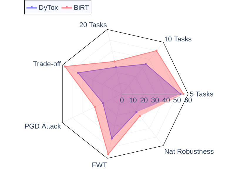
Figure 1: Overall performance of our proposed method, BiRT, vs. DyTox trained continually on CIFAR-100 with 500 buffer size on different metrics; Top-1 accuracy is reported for all metrics. Therefore, a CL method with full coverage of the octagon has all the ideal features: highest accuracy (on varying task sequences), natural/adversarial robustness, forward transfer, and stability-plasticity trade-off.

Computational systems operating in the real world are normally exposed to a sequence of multiple tasks with non-stationary data streams. Similar to biological organisms, it is desirable for these artificial systems to be able to learn on a continual basis to successfully act and adapt to new scenarios in the real world. However, deep neural networks (DNNs) are inherently designed for training on stationary, independent, and identically distributed (i.i.d.) data. The sequential nature of continual learning (CL) violates this strong assumption, leading to catastrophic forgetting of older tasks. Catastrophic forgetting often leads to a rapid decline in the performance of old tasks and, in the worst case, the previously acquired information is completely overwritten by the new one (Parisi et al.,, 2019).

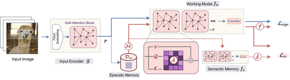
Figure 2: BiRT employs a bio-inspired non-veridical experience replay in a dual memory system based on vision transformers. The semantic memory, $f_{s}$, gradually assimilates learned knowledge from working model, $f_{w}$, by taking an exponential moving average over its weights. The semantic memory interacts with the episodic memory which stores the learned representations of the previous tasks ($r$). To effectively replay these abstract high-level representations, we inject constructive noise by mixing up representations ($\tilde{\mathcal{M}}$), adding noise to the internal attention maps ($\tilde{\mathcal{A}}$), and emulating trial-to-trial variability through adding noise to the outputs of semantic memory ($\tilde{\mathcal{S}}$) and to the targets ($\tilde{\mathcal{T}}$). To retrieve the knowledge, the consolidated knowledge from semantic memory is enforced to the working model in the functional space via a consistency regularization.

Rehearsal-based approaches, which store and replay previous task samples, have been fairly successful in mitigating catastrophic forgetting in CL. Recent evidence suggests that replay might even be unavoidable in certain CL scenarios (Farquhar and Gal,, 2018). However, replaying raw pixels from past experiences is not consistent with neurophysiological mechanisms in the brain (Kudithipudi et al.,, 2022; Hayes et al.,, 2019). Furthermore, the replay of raw pixels is memory inefficient and raises data privacy and security concerns (Mai et al.,, 2022). Juxtaposing biological and artificial experience rehearsal, representation rehearsal is a lucrative alternative to address the problems associated with raw image rehearsal in CL. Representation rehearsal, either generative (van de Ven et al.,, 2020; Lao et al.,, 2020) or by storing (Hayes et al.,, 2020; Caccia et al.,, 2020; Iscen et al.,, 2020), entails replaying the latent features of the intermediate layers of DNNs to mitigate catastrophic forgetting. In generative methods, the generator itself is as large as the CL model and is prone to catastrophic forgetting. Additionally, generative models are difficult to train and suffer mode collapse. However, although storing representations is memory and computation efficient, choosing an ideal layer for rehearsal remains an open question. Furthermore, stored representations in a bounded memory lack diversity, resulting in overfitting.

In contrast, the human brain learns, stores, and remembers experiences without catastrophically forgetting previous tasks. The versatility of the brain can be attributed to the rehearsal of abstract experiences through multiple memory systems (Hassabis et al.,, 2017) and a rich set of neurophysiological processing principles (Parisi et al.,, 2019). In addition, the brain harbors random disturbances of signals, termed noise, that contribute to cellular and behavioral trial-to-trial variability (Faisal et al.,, 2008). Although noise is sometimes considered a nuisance, noise forms a notable component of the computational strategy of the brain. The brain exploits noise to perform tasks, such as probabilistic inference through sampling, that facilitate learning and adaptation in dynamic environments (Maass,, 2014). As is the case in the brain, we hypothesize that noise can be a valuable tool in improving generalization in representation rehearsal in vision transformers.

To this end, we propose BiRT, a novel representation rehearsal-based continual learning method based on vision transformers, architectures composed of self-attention modules inspired by human visual attention (Lindsay,, 2020). Specifically, our method consists of two complementary learning systems: a working model and semantic memory, an exponential moving average of the working model. To reduce overfitting and bring diversity in representation rehearsal, BiRT introduces various controllable noises at various stages of the vision transformer and enforces consistency in predictions with respect to semantic memory. As semantic memory consolidates semantic information, consistency regularization in the presence of meaningful noise promotes generalization while effectively reducing overfitting. BiRT provides a consistent performance gain over the raw image and the vanilla representation rehearsal on several CL scenarios and metrics while being robust to natural and adversarial corruptions (Figure 1).

2 Related Work

Continual Learning: DNNs are typically designed to incrementally adapt to stationary i.i.d. data streams shown in isolation and random order (Parisi et al.,, 2019). Therefore, sequential learning over non-i.i.d. data causes catastrophic forgetting of previous tasks and overfitting of the current task. Approaches to address catastrophic forgetting can be broadly divided into three categories: regularization-based approaches (Kirkpatrick et al.,, 2017; Zenke et al.,, 2017; Li and Hoiem,, 2017) penalize changes in important parameters pertaining to previous tasks, parameter isolation methods (Rusu et al.,, 2016; Aljundi et al.,, 2017; Fernando et al.,, 2017) allocate a distinct set of parameters for distinct tasks, and rehearsal-based approaches (Ratcliff,, 1990; Rebuffi et al.,, 2017; Lopez-Paz and Ranzato,, 2017; Bhat et al.,, 2023) store old task samples and replay them alongside current task samples. Among different approaches to mitigate catastrophic forgetting, experience rehearsal is fairly successful in multiple CL scenarios (Parisi et al.,, 2019).

Rehearsal-based approaches replay raw pixels from past experiences, inconsistent with how humans continually learn (Kudithipudi et al.,, 2022). Furthermore, the replay of raw pixels can have other ramifications, including a large memory footprint, data privacy, and security concerns (Mai et al.,, 2022). Therefore, several works (Pellegrini et al.,, 2020; Iscen et al.,, 2020; Caccia et al.,, 2020) mimic abstract representation rehearsal in the brain by storing and replaying representations from intermediate layers in DNNs. Representation rehearsal can be done by employing generative models (van de Ven et al.,, 2020; Lao et al.,, 2020) or by storing previous task representations in the buffer (Hayes et al.,, 2020; Iscen et al.,, 2020). While generative models themselves are prone to forgetting and mode collapse, storing representations in a bounded memory buffer lacks diversity due to the unavailability of proper augmentation mechanisms. Although high-level representation replay can potentially mitigate memory overhead and privacy concerns, replaying representations over and over again leads to overfitting.

Transformers for CL: Transformer architectures (Vaswani et al.,, 2017) were first developed for machine translation and later expanded to computer vision tasks (Dosovitskiy et al.,, 2020; Touvron et al.,, 2021; Jeeveswaran. et al.,, 2022) by considering image patches as replacements for tokens. Despite their success in several benchmarks, vision transformers have not been widely considered for continual learning. Yu et al., (2021) studied transformers in a class-incremental learning setting and pointed out several problems in naively applying transformers in CL. DyTox (Douillard et al.,, 2021) proposed a dynamically expanding architecture using separate task tokens to model the context of different classes in CL. LVT (Wang et al., 2022a, ) proposed an external key and an attention bias to stabilize the attention map between tasks and used a dual classifier structure to avoid catastrophic interference while learning new tasks. Pelosin et al., (2022) proposed an asymmetric regularization loss on pooled attention maps with respect to the model learned on the previous task to continually learn in an exemplar-free approach. Several other concurrent works (Ermis et al.,, 2022; Wang et al., 2022c, ; Wang et al., 2022b, ) harnessed the pre-trained model and incorporated the learning of generic and task-specific parameters. Unlike these works, we do not use pre-trained models and replay intermediate representations instead of raw image inputs.

We seek to improve the performance of vision transformers under representation rehearsal in CL. As noise plays a constructive role in the brain, we mimic the prevalence of noise in the brain and the consequent trial-to-trial variability by injecting noise into our proposed method.

3 Proposed Method

The CL paradigm normally consists of $T$ sequential tasks, with the data gradually becoming available over time. During each task $t\in\{1,2,..,T\}$, the samples and the corresponding labels $(x_{i},y_{i})_{i=1}^{N}$ are drawn from the task-specific distribution $\mathcal{D}_{t}$. The continual learning model $f_{\theta}$ is optimized sequentially on one task at a time, and inference is carried out on all the tasks seen so far. CL is especially challenging for vision transformers due to the limited training data for every task (Raghu et al.,, 2021; Touvron et al.,, 2021) in addition to the issue of catastrophic forgetting. By mimicking the association of past and present experiences in the brain, experience rehearsal (ER) partially addresses the problem of catastrophic forgetting. Thus, the learning objective of ER is as follows:

$$\begin{split}\mathcal{L}_{er}\triangleq\displaystyle&\mathop{\mathbb{E}}_{(x_{i},y_{i})\sim\mathcal{D}_{t}}\left[\>\mathcal{L}_{ce}(f_{\theta}({x}_{i}),y_{i})\>\right]\\ &+\alpha\displaystyle\mathop{\mathbb{E}}_{(x_{j},y_{j})\sim\mathcal{D}_{m}}\left[\;\mathcal{L}_{ce}(f_{\theta}({x}_{j}),y_{j})\;\right],\end{split}$$ (1)

where $\alpha$ represents a balancing parameter, $\mathcal{D}_{m}$ is episodic memory, and $\mathcal{L}_{ce}$ is cross-entropy loss. To further reduce catastrophic forgetting, we employ a complementary learning system based on abstract, high-level representation rehearsal. To promote diversity and generalization in representation rehearsal, we introduce various controllable noises at different stages of the vision transformer and enforce consistency in predictions with respect to the semantic memory. In the following sections, we describe in detail different components of BiRT.

3.1 Knowledge Consolidation through complementary learning system

Complementary learning system (CLS) theory posits that the hippocampus and neocortex entail complementary properties necessary to capture complex interactions in the brain (McNaughton and O’Reilly,, 1995). Inspired by CLS theory, we propose a dual memory transformer-based learning system that acquires and assimilates knowledge over short and long periods of time. The working model encounters new tasks and consolidates knowledge over short periods of time. We then gradually aggregate the weights of the working model into semantic memory during intermittent stages of inactivity. Following Arani et al., (2021), we design the semantic memory as an exponential moving average of the working model as follows:

$$\theta_{s}=\gamma\theta_{s}+(1-\gamma)\theta_{w}$$ (2)

where $\theta_{w}$ and $\theta_{s}$ are the weights of the working model and semantic memory, respectively, and $\gamma$ is a decay parameter. As the working model focuses on specializing on the current task, the copy of the working model at each training step can be considered as an expert on a particular task. Therefore, the aggregation of weights throughout CL training can be deemed as an ensemble of expert models that consolidate knowledge across tasks, resulting in smoother decision boundaries.

3.2 Episodic Memory

In line with experience rehearsal in the brain (Ji and Wilson,, 2007), we propose an abstract, high-level representation rehearsal for vision transformers. The working model comprises two nested functions: $g(.)$ and $f_{w}(.)$. The first few layers of the encoder, $g(.)$, process the raw image input, and the output along with the ground truth label is stored in episodic memory $\mathcal{D}_{m}$. To ensure consistency in intermediate representations, $g(.)$ can be initialized using pre-trained weights and fixed before starting CL training or fixed after learning some tasks. On the other hand, $f_{w}(.)$, the later layers of the transformer, process abstract high-level representations, and remain learnable throughout the CL training. During intermittent stages of inactivity, the stable counterpart semantic memory $f_{s}(.)$ is updated according to Eq. 2.

The episodic memory is populated at the task boundary using iCaRL herding (Rebuffi et al.,, 2017). Representations $r_{j}=g(x_{j})$, stored in episodic memory, are interleaved with current task representations and are processed synchronously by $f_{w}(.)$ and $f_{s}(.)$. The learning objective for representation rehearsal can thus be obtained by adapting Eq. 1 as follows:

$$\begin{split}\mathcal{L}_{repr}\triangleq\displaystyle\mathop{\mathbb{E}}_{(x_{i},y_{i})\sim\mathcal{D}_{t}}\left[\>\mathcal{L}_{ce}(f_{w}(g(x_{i})),y_{i})\>\right]\\ +\;\alpha\displaystyle\mathop{\mathbb{E}}_{(r_{j},y_{j})\sim\mathcal{D}_{m}}\left[\;\mathcal{L}_{ce}(f_{w}(r_{j}),y_{j})\;\right]\end{split}$$ (3)

Algorithm 1 BiRT Algorithm

  input: Data streams $\mathcal{D}_{t}$, buffer $\mathcal{D}_{m}$, working model $f_{w}$, hyperparameters $\gamma$, $\alpha_{t}$, $\alpha_{m}$, $\alpha_{a}$, $\alpha_{s}$

  for all tasks $t\in\{1,2,..,T\}$ do

     for epochs $e\in\{1,2,..,E\}$ do

        sample a mini-batch ${(x,y)}\sim\mathcal{D}_{t}$

        $x=augment(x)$

        if $\mathcal{D}_{m}\neq\emptyset$ then

           sample a mini-batch ${(r,y)}\sim\mathcal{D}_{m}$

           $a,b,c,d,e\sim\mathcal{U}(0,1)$

           $\tilde{y}\leftarrow\tilde{\mathcal{T}}(y)$                  if $a<\alpha_{t}$

           $(\tilde{r},\tilde{y})\leftarrow\tilde{\mathcal{M}}(r,y)$      if $b<\alpha_{m}$      $\blacktriangleright$ (Eq. 4)

           $\tilde{A}\leftarrow\tilde{\mathcal{A}}(A)$                if $c<\alpha_{a}$      $\blacktriangleright$ (Eq. 5)

           $f_{s}(r)\leftarrow\tilde{\mathcal{S}}(f_{s}(r),\delta)$  if $d<\alpha_{s}$      $\blacktriangleright$ (Eq. 7)

        end if

        Compute outputs of $f_{w}(.)$ and $f_{s}(.)$

        Compute $\mathcal{L}=\mathcal{L}_{repr}+\rho\mathcal{L}_{cr}\;$       $\blacktriangleright$ (Eqs. 3, 6, 8)

        $\theta_{w}\leftarrow\theta_{w}+\nabla_{\theta_{w}}\mathcal{L}$

        $\theta_{s}\leftarrow\gamma\theta_{s}+(1-\gamma)\theta_{w}$  if $e<\alpha_{e}$ and $t>1$

     end for

     if task-end = True then

        if t = 1 then

           Freeze $g(.)$

           $\theta_{s}=\text{copy}(\theta_{w})$

        end if

        $\mathcal{D}_{m}\leftarrow(r,y)$

     end if

  end for

  Return:working model $\theta_{w}$, and semantic memory $\theta_{s}$

3.3 Noise and Trial-to-Trial Variability

Noise is prevalent at every level of the nervous system and has recently been shown to play a constructive role in the brain (Faisal et al.,, 2008; McDonnell and Ward,, 2011). Trial-to-trial variability, a common phenomenon in biological systems in which the neural response to the same stimuli differs across trials, is often the result of noise (Faisal et al.,, 2008). Trial-to-trial variability has been shown to be one of the key components of the computational mechanism in the brain (Maass,, 2014). Furthermore, injecting noise into the neural network learning pipeline has been shown to result in faster convergence to the global optimum (Zhou et al.,, 2019), better generalization (Srivastava et al.,, 2014), and effective knowledge distillation.

To simulate noise and trial-to-trial variability, we stochastically inject constructive noise into various components of our CL setup. In the following sections, we describe in detail how exactly we leverage noise during CL training.

Table 1: Results on multiple datasets learned with 10 tasks with varying buffer sizes, averaged over multiple class orders. BiRT achieves consistent improvements over DyTox in different metrics, i.e. accuracy, forgetting, BWT, and FWT. The last accuracy determines the performance on past tasks after learning the last task, and the average accuracy shows the average of the last accuracy after learning every task.

	Buffer Size		500		1000		2000
		Joint	DyTox	BiRT	DyTox	BiRT	DyTox	BiRT
CIFAR-100	Last Acc $\uparrow$	74.99$\pm$0.22	34.54$\pm$1.82	50.20$\pm$0.67	43.92$\pm$0.84	51.20$\pm$1.46	52.34$\pm$0.46	53.01$\pm$0.57
	Avg Acc $\uparrow$		58.35$\pm$1.54	63.82$\pm$1.80	63.67$\pm$1.31	64.56$\pm$2.31	68.42$\pm$1.13	66.70$\pm$0.36
	BWT $\uparrow$		-39.79$\pm$1.16	-15.62$\pm$0.29	-32.05$\pm$0.33	-15.25$\pm$0.66	-24.44$\pm$0.65	-16.30$\pm$1.31
	FWT $\uparrow$		41.51$\pm$1.61	56.14$\pm$1.52	50.04$\pm$1.17	57.04$\pm$2.2	57.77$\pm$0.77	59.74$\pm$1.30
	Forgetting $\downarrow$		53.87$\pm$1.95	17.45$\pm$0.61	43.64$\pm$0.71	17.70$\pm$1.42	33.92$\pm$0.79	19.00$\pm$1.98
TinyImageNet	Last Acc $\uparrow$	58.46$\pm$0.60	23.95$\pm$0.71	32.60$\pm$.018	33.25$\pm$1.28	38.41$\pm$0.33	37.34$\pm$0.22	40.49$\pm$0.52
	Avg Acc $\uparrow$		42.53$\pm$1.74	44.57$\pm$2.84	48.74$\pm$1.29	49.26$\pm$2.34	51.30$\pm$2.17	51.15$\pm$0.34
	BWT $\uparrow$		-40.46$\pm$0.41	-13.38$\pm$0.98	-31.12$\pm$1.19	-17.34$\pm$0.51	-27.68$\pm$0.77	-17.85$\pm$0.37
	FWT $\uparrow$		27.84$\pm$1.02	37.87$\pm$1.91	36.60$\pm$0.34	41.97$\pm$1.54	40.39$\pm$1.16	43.93$\pm$1.54
	Forgetting $\downarrow$		52.32$\pm$0.94	14.57$\pm$2.00	40.07$\pm$2.12	18.85$\pm$0.22	35.56$\pm$1.29	19.48$\pm$0.21
ImageNet-100	Last Acc $\uparrow$	79.05$\pm$0.16	39.03$\pm$1.57	51.05$\pm$0.24	50.62$\pm$1.04	52.89$\pm$0.96	58.54$\pm$0.42	59.52$\pm$1.39
	Avg Acc $\uparrow$		60.52$\pm$1.56	65.51$\pm$0.30	68.14$\pm$1.38	67.33$\pm$0.57	71.67$\pm$1.71	70.51$\pm$1.87
	BWT $\uparrow$		-38.15$\pm$0.48	-14.42$\pm$0.06	-26.87$\pm$0.72	-12.90$\pm$0.31	-21.10$\pm$0.78	-16.53$\pm$0.84
	FWT $\uparrow$		44.94$\pm$1.69	58.27$\pm$0.30	56.86$\pm$1.46	60.78$\pm$0.86	62.85$\pm$1.54	63.40$\pm$2.01
	Forgetting $\downarrow$		51.71$\pm$0.91	16.10$\pm$0.42	37.93$\pm$11.23	14.83$\pm$0.67	28.68$\pm$1.41	19.79$\pm$0.61

3.3.1 Representation noise $\mathcal{\tilde{M}}$

During CL training, the working model encounters task-specific data $\mathcal{D}_{t}$ that are first fed into $g(.)$, and then the output representations of $g(.)$ are interleaved with the representations of previous task samples from episodic memory $\mathcal{D}_{m}$. We update $\mathcal{D}_{m}$ at the task boundary using iCaRL herding. The interleaved representations are then processed by both $f_{w}(.)$ and $f_{s}(.)$. Analogous to the replay of novel samples in the brain (Liu et al.,, 2019), we linearly combine representations sampled from episodic memory using a manifold mixup (Verma et al.,, 2019):

$$\begin{split}\tilde{r}&=\lambda r_{i}+(1-\lambda)\;r_{j}\\ \tilde{y}&=\lambda y_{i}+(1-\lambda)\;y_{j},\end{split}$$ (4)

where $r_{i},r_{j}$ are stored representations of two different samples and $y_{i},y_{j}$ are the corresponding labels. Here, the mixing coefficient $\lambda$ is drawn from a Beta distribution. As manifold mixup interpolates representations of samples belonging to different classes / tasks, it brings diversity for the experience-rehearsal, thereby reducing overfitting.

3.3.2 Attention noise $\mathcal{\tilde{A}}$

As we employ vision transformer as our architecture of choice, self-attention forms the core component of BiRT. The working model $f_{w}(.)$ in BiRT consists of several multi-head self-attention layers that map a query and a set of key-value pairs to an output. We inject noise into the scaled dot-product attention at each layer of $f_{w}(.)$ while replaying the representation as follows:

$$\operatorname{Attention}(Q,K,V)=(\operatorname{softmax}\left(\frac{QK^{T}}{\sqrt{d_{k}}}\right)+\epsilon)\;V$$ (5)

where $Q$, $K$ and $V$ are query, key and value matrices, and $\epsilon\sim\mathcal{N}(0,\sigma^{2})$ is a white Gaussian noise. By stochastically injecting noise into self-attention, we discourage BiRT from attending to sample specific features, thereby potentially mitigating overfitting.

3.3.3 Supervision noise $\mathcal{\tilde{T}}$ and $\mathcal{\tilde{S}}$

We now shift our focus toward the supervision signals to further reduce overfitting in CL. Due to over-parameterization, the CL model tends to overfit on the limited number of samples from the buffer. Therefore, we introduce a synthetic label noise ($\mathcal{\tilde{T}}$) wherein a small percentage of the samples are re-assigned a random class. BiRT takes advantage of the fact that label noise is sparse, meaning that only a fraction of the labels are corrupted while the rest are intact in the real world (Liu et al.,, 2022). In addition, the harmful effects of inherent label noise on generalization can be mitigated by using additional controllable label noise (Chen et al.,, 2021).

During intermittent stages of inactivity, the knowledge in the working model is consolidated into semantic memory through Eq. 2. Therefore, knowledge of previous tasks is encoded in semantic memory weights during the learning trajectory of the working model (Hinton et al.,, 2015). Then, to retrieve the structural knowledge encoded in the semantic memory, we regularize the function learned by the working model by enforcing consistency in its predictions with respect to the semantic memory:

$$\begin{split}\mathcal{L}_{cr}\triangleq\beta_{1}&\displaystyle\mathop{\mathbb{E}}_{x_{i}\sim D_{t}}\lVert f_{w}(g(x_{i}))-f_{s}(g(x_{i}))\rVert_{p}\\ &+\beta_{2}\displaystyle\mathop{\mathbb{E}}_{r_{j}\sim D_{m}}\lVert f_{w}(r_{j})-f_{s}(r_{j})\rVert_{p},\end{split}$$ (6)

where $\beta_{1}$ and $\beta_{2}$ are balancing weights. To mimic trial-to-trial variability in the brain, we inject noise into the logits of semantic memory ($\mathcal{\tilde{S}}$) before applying consistency regularization as follows:

$$f_{s}(r_{j})\leftarrow f_{s}(r_{j})+\delta$$ (7)

where $\delta\sim\mathcal{N}(0,\sigma^{2})$ is a white Gaussian noise, $\mathcal{L}_{cr}$ represents the expected Minkowski distance between the corresponding pairs of predictions and $p=2$. Consistency regularization enables the working model to retrieve structural knowledge from the semantic memory from previous tasks. Consequently, the working model adapts the decision boundary to new tasks without catastrophically forgetting previous tasks.

Thus, the final learning objective for the working model is as follows:

$$\mathcal{L}\triangleq\mathcal{L}_{repr}+\rho\;\mathcal{L}_{cr}$$ (8)

where $\rho$ is a balancing parameter. Our proposed approach is illustrated in Figure 2 and is detailed in Algorithm 1.

Note that these noises are applied stochastically, and therefore, a single representation can have multiple noises associated with it. Although noise is generally treated as a nuisance, BiRT introduces controllable noise at various stages of the vision transformer to promote robust generalization in CL.

Table 2: Results on CIFAR-100 learned with 5, 10, and 20 tasks with varying buffer sizes. BiRT achieves consistent improvements over the state-of-the-art on average accuracy and last accuracy.

Methods	Buffer Size	#P	5 steps		10 steps		20 steps
			Avg	Last	Avg	Last	Avg	Last
ATT-asym	-	16.87	-	-	25.58 $\pm$0.01	16.31 $\pm$0.00	-	-
FUNC-asym	-	16.87	-	-	25.95 $\pm$0.00	16.21 $\pm$0.01	-	-
BiRT	-	10.73	-	-	56.40 $\pm$1.57	42.59 $\pm$0.84	-	-
DyTox		10.73	56.98 $\pm$0.61	41.50 $\pm$1.00	48.31 $\pm$1.23	23.92 $\pm$1.11	38.10 $\pm$1.72	14.27 $\pm$0.94
LVT	200	8.9	-	39.68 $\pm$1.36	-	35.41 $\pm$1.28	-	20.63 $\pm$1.14
BiRT		10.73	67.15 $\pm$0.95	54.15 $\pm$0.94	61.01 $\pm$1.58	45.59 $\pm$1.54	48.03 $\pm$0.97	29.10 $\pm$1.88
DyTox		10.73	63.85 $\pm$0.99	52.99 $\pm$0.53	58.35 $\pm$1.54	34.54 $\pm$1.82	49.98 $\pm$1.32	24.86 $\pm$0.81
LVT	500	8.9	-	44.73 $\pm$1.19	-	43.51 $\pm$1.06	-	26.75 $\pm$1.29
BiRT		10.73	68.40 $\pm$1.56	55.65 $\pm$0.99	63.82 $\pm$1.80	50.20 $\pm$0.67	50.34 $\pm$1.64	30.22 $\pm$1.63

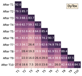
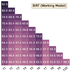
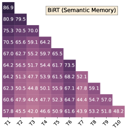
Figure 3: Comparison of task-wise performance after learning each task on CIFAR-100 with a buffer size of 500 learned for 10 tasks. The working model achieves better accuracy for the seen tasks after learning 10 tasks compared to DyTox. The semantic memory retains the performance of older tasks better than DyTox and the working model.

4 Experimental Results

We use the continuum library (Douillard and Lesort,, 2021) to implement different CL scenarios and build our approach on top of DyTox (Douillard et al.,, 2021) method, the main baseline in all our experiments. We report the last accuracy (Last), average accuracy (Avg), forward transfer (FWT), backward transfer (BWT) and forgetting. More information on experimental setup, datasets, and metrics can be found in Appendix A.

Table 1 presents the comparison of our method with standard CL benchmarks with different buffer sizes, averaged across three random seeds. We can make the following observations from Table 1: (i) Across CL settings and different buffer sizes, BiRT shows consistent performance improvement over DyTox across all metrics. (ii) BiRT enables the consolidation of rich information about the previous tasks better even under low buffer regimes, e.g. for CIFAR-100, the absolute improvement in terms of Last Acc is $7.28\%$ for buffer size 1000 while it is as much as $15.66\%$ for buffer size 500. (iii) BWT and FWT elucidate the influence of learning a new task $t$ on the performance of previous and subsequent tasks, respectively. BiRT shows a smaller negative BWT and a higher positive FWT across all CL datasets, resulting in less forgetting and better forward facilitation. (iv) TinyImageNet is one of the challenging datasets for CL considered in this work. Under low buffer regimes, the number of samples per class will be severely limited due to the large number of classes per task. BiRT consistently outperforms DyTox across all buffer sizes on TinyImageNet.

Table 2 further demonstrates the comparison of our method with transformer-based exemplar-free (ATT-asym and FUNC-asym (Pelosin et al.,, 2022); averaged over 3 seeds) and rehearsal-based (DyToX and LVT; averaged over 5 class orderings) approaches. Although originally not designed for the exemplar-free scenario, BiRT shows a significant improvement over the rehearsal-free methods. Progressing from the exemplar-free scenario, BiRT shows a further improvement in performance when provided with experience rehearsal. We also compare CL methods with different numbers of tasks in CIFAR-100 with limited buffer sizes. BiRT consolidates generalizable features rather than discriminative features specific to buffered samples, thereby exhibiting superior performance across all buffer sizes and task sequences.

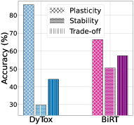
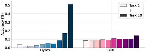
Figure 4: Comparison of CL methods in the stability-plasticity trade-off (left) and the task-recency bias (right) on C-100 (buffer size 500).

Reinforcing our earlier hypothesis, the controllable noises introduced in BiRT play a constructive role in promoting generalization and consequently reducing overfitting in CL. In addition to allaying privacy concerns, replacing raw image rehearsal with representation rehearsal reduces the memory footprint without compromising performance.

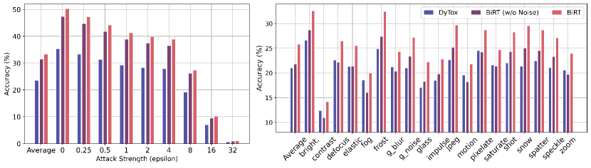
Figure 5: Robustness of CL methods to adversarial attacks (left) and 19 different natural corruptions (right) on C-100 (buffer size 500).

5 Model Analysis

Task Recency Bias: Sequential learning of multiple tasks causes classifier predictions to tilt toward recent tasks, resulting in a task recency bias (Masana et al.,, 2020). One direct consequence of task recency bias is that the classifier norm is higher for recent classes while lower for older classes, which means that older classes are less likely to be picked for prediction (Hou et al.,, 2019). Following the analysis in (Bhat et al.,, 2022), Figure 4 (right) shows the normalized probability that all classes in each task are predicted at the end of training. The probabilities in BiRT are more evenly distributed than in DyTox, resulting in a lower recency bias. We argue that supervision noises proposed in BiRT implicitly regularize the classifier towards more evenly distributed prediction probabilities.

Stability-Plasticity Dilemma: The extent to which the CL model is plastic enough to acquire new information while stable enough not to catastrophically interfere with consolidated knowledge is referred to as stability-plasticity dilemma (Parisi et al.,, 2019). Catastrophic forgetting is a direct consequence of this dilemma when the plasticity of the CL model overtakes its stability. To investigate how well our method handles the stability-plasticity dilemma, we plot the task-wise performance at the end of each task in Figure 3 for the CIFAR-100 test set. Following Sarfraz et al., (2022), we also visualize a formal trade-off measure in Figure 4 (left). Both the working model and semantic memory exhibit higher stability, while DyTox is more plastic. Therefore, DyTox is more prone to forgetting, whereas BiRT displays a better stability-plasticity trade-off compared to the baseline.

Attention Map Analysis: As learning progresses through a sequence of tasks, a CL model that retains its focus on salient regions undergoes less catastrophic forgetting. Therefore, it would be beneficial to study the variation in the salient regions of the image during the learning trajectory. Figure 6 shows a comparison of saliency maps for samples of the first task after training on the first and last task, respectively. As can be seen, BiRT retains the attention to important regions in these images better than DyTox. We contend that the attention noise proposed in BiRT helps focus on class-wide features rather than sample specific features, thereby retaining attention to important regions in test images. More explanation and extended visualizations are provided in Appendix M.

Robustness Analysis: Continual learning models are mostly evaluated on accuracy on seen tasks and forgetting metrics. However, the research community has largely neglected the susceptibility of continually learned models to adversarial attacks and corrupted data in the wild (Khan et al.,, 2022). Figure 5 illustrates the robustness of BiRT on adversarial attack of varying strengths (Kim,, 2020) and several natural corruptions (Hendrycks and Dietterich,, 2019). In addition, we evaluate the robustness of BiRT without any noise in the learning trajectory in order to elucidate the benefits of constructively inducing noise in the pipeline of continually learning models. BiRT is robust to adversarial attacks, as well as corrupted data, and learning with noise results in improved robustness. This is evident from the performance under severe noises such as ‘contrast’, ‘fog’, ‘motion blur’ and the average performance across different settings wherein learning with noise helps the model recover from the inferior performance.

This makes it well-suited for safety-critical applications, such as autonomous vehicles, where the consequences of a model failure can be severe.

6 Ablation Study

Table 3 provides an overview of the effect of the different components used in BiRT. Unlike DyTox, we employ an exponential moving average as semantic memory, resulting in the biggest jump in accuracy. BiRT entails representation, attention, and supervision noises to promote robust generalization in CL and diversify the buffered representations. As can be seen, all three components of BiRT play a constructive role in building a successful continual learner. Supervision noise, representation noise, and attention noise bring performance improvements of 0.54%, 3.30%, and 3.41%, respectively, over BiRT without any noise. In addition, compared to vanilla representation rehearsal, the right combination of controllable noises in BiRT greatly reduces overfitting and improves performance by as much as $9\%$ (relative Avg). Therefore, it is quintessential to have controllable noise to further improve representation rehearsal in CL.

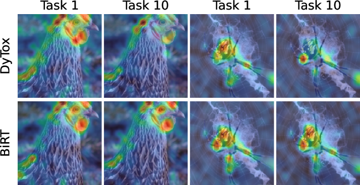
Figure 6: Comparison of attention maps on the validation set of the first task of ImageNet-100 trained for 10 tasks with buffer size 500 (red regions correspond to regions with higher attention). BiRT retains the knowledge of salient regions in the image better than DyTox, leading to better predictions and less forgetting.

Table 3: Ablations of the different key components of BiRT. The average and last accuracies are reported on CIFAR100 for the buffer size of 500 learned for 10 tasks.

Supervision Noise	Repres. Noise	Attention Noise	Last Acc	Avg Acc
✓	✓	✓	50.20$\pm$0.67	63.82$\pm$1.80
✗	✓	✓	49.63$\pm$0.30	63.67$\pm$1.55
✗	✗	✓	49.30$\pm$0.91	63.29$\pm$1.71
✓	✗	✗	49.19$\pm$0.46	62.58$\pm$1.44
✗	✓	✗	46.43$\pm$0.41	61.83$\pm$0.23
✗	✗	✗	45.89$\pm$1.25	59.58$\pm$0.58
DyTox			34.54$\pm$1.82	58.35$\pm$1.54

7 Conclusions and Future Work

We proposed BiRT, a novel representation rehearsal-based continual learning approach based on vision transformers. Specifically, we introduce controllable noises at various stages of the vision transformer and enforce consistency in predictions with respect to an exponential moving average of the working model. Our empirical results show that BiRT outperforms raw image rehearsal and vanilla representation rehearsal while being memory efficient and robust to natural and adversarial corruptions. Furthermore, the improvement is even more pronounced under low buffer regimes and longer task sequences. Reinforcing our earlier hypothesis, the controllable noises introduced in BiRT play a constructive role in promoting generalization and consequently reducing overfitting in CL. Extending our work to more realistic settings such as general CL where task boundaries are not known at training time, and exploring other efficient transformer architectures are some of the useful research directions for this work.

Appendix A Experimental setup, datasets and metrics

We use the continuum library (Douillard and Lesort,, 2021) to implement different CL scenarios and build our approach on top of DyTox (Douillard et al.,, 2021) framework, which is the main baseline in all our experiments. We use a network that consists of 5 self-attention blocks and a task-attention block. All blocks have 12 attention heads and an embedding dimension of 384. We train models with a learning rate of $5e^{-4}$, a batch size of 128, and a weight decay of $1e^{-6}$. All models, including the baseline, are trained for 500 epochs per task in CIFAR-100 (Krizhevsky et al.,, 2009), TinyImageNet (Le and Yang,, 2015), and ImageNet-100 (Deng et al.,, 2009). During the patch embedding process, we utilize patch sizes of 4 for CIFAR-100, 8 for TinyImageNet, and 16 for ImageNet-100. After each task, the model is fine-tuned on a balanced dataset with a learning rate of $5e^{-5}$ for 20 epochs. All models are trained on a single NVIDIA V100 GPU, and all evaluations are performed on a single NVIDIA RTX 2080 Ti GPU.

We focus mainly on the class-incremental learning setting (Class-IL) (Van de Ven and Tolias,, 2019), where the task ID is not known at the test time. In every task, samples belonging to a new set of classes disjoint from the previous tasks’ classes are learned by the model. Following Douillard et al., (2021) and De Lange et al., (2021), we evaluate our approach on CIFAR-100, ImageNet-100, and TinyImageNet. CIFAR-100 consists of 50,000 training images and 10,000 test images of size 32$\times$32 belonging to 100 classes. ImageNet-100 consists of 129k train and 5,000 validation images of size 224$\times$224 belonging to 100 classes. TinyImageNet consists of 100,000 training images and 10,000 test images of size 96$\times$96 belonging to 200 classes.

Except for the analysis of longer task sequences, all other experiments are carried out in the Class-IL setting with 10 tasks. In the case of CIFAR-100, 100 classes are divided into 10 tasks, with 10 classes in each task. Similarly, 20 classes per task are learned on TinyImageNet and 10 classes per task on ImageNet-100. The order in which classes are learned can affect the performance of a CL model (Yoon et al.,, 2019). We use “class order 1” from (Douillard et al.,, 2021) for CIFAR-100 and ImageNet-100, and the sequential class order from 1 to 200 for TinyImageNet-200.

Although the performance of task-incremental learning (Task-IL) can be evaluated in our proposed approach, we exclude them in our analysis because it simplifies the CL scenario by assuming the availability of task id at the test time, which translates into choosing the right prediction head during inference.

A.1 Evaluation Metrics

To evaluate the performance of different models under different settings, we select five different metrics widely used in the CL literature. We formalize each metric below.

1. Last Accuracy (Douillard et al.,, 2021) defines the final performance of the CL model on the validation set of all the tasks seen so far. Concretely, given that tasks are sampled from a set $t\in{1,2...,T}$, where $T$ is the total number of tasks and $a_{k,j}$ is the accuracy of a CL model on the validation set of the task $k$ after learning task $j$, last accuracy $A_{last}$ is as follows:

   $$A_{last}=\frac{1}{T}\sum_{k=1}^{T}a_{k,T}$$ (9)

2. Average Accuracy (Rebuffi et al.,, 2017) defines the average performance of the learned CL model on the validation set of all tasks seen so far after learning each task. Given that $K$ is the number of tasks seen so far and $T$ is the total number of tasks, the average accuracy $A_{avg}$ is as follows:

   $$A_{avg}=\frac{1}{T}\sum_{j=1}^{T}\frac{1}{K}\sum_{k=1}^{K}a_{k,j}$$ (10)

3. Backward Transfer (BWT) (Lopez-Paz and Ranzato,, 2017) defines the influence of the learning task $t$ on previously seen tasks $k<t$. Positive BWT implies that the learning task $t$ increased performance on previous tasks, while negative BWT indicates that the learning task $t$ affected the performance of the model on previous tasks. Formally, BWT is as follows:

   $$BWT=\frac{1}{T-1}\sum_{j=1}^{T-1}a_{T,j}-a_{j,j}$$ (11)

4. Forward Transfer (FWT) (Lopez-Paz and Ranzato,, 2017) defines the influence of learning the task $t$ on future tasks $k>t$. Positive FWT implies that learning the task $t$ increased performance in future tasks and vice versa. Positive FWT occurs when the model learns generalizable features that can help it learn future tasks. Formally, given that $\hat{a}_{j}$ is the accuracy of the task $j$ at random initialization, the FWT is as follows:

   $$FWT=\frac{1}{T-1}\sum_{j=2}^{T}a_{j-1,j}-\hat{a}_{j}$$ (12)

5. Forgetting (Chaudhry et al.,, 2018) quantifies the forgetting of previously learned tasks given the current state of the model. It is defined as the difference between the maximum accuracy of the model in previously learned tasks throughout the learning process and the current accuracy of the task. Concretely, forgetting for the task $k$ is as follows:

   $$\text{Forgetting}=\max_{l\in{1,2,...,k-1}}a_{k,l}-a_{k,T}$$ (13)

Appendix B Quantitative results for figures

To facilitate comparisons with BiRT, we provide quantitative results for the figures in the main text.

B.1 Effect of Longer Sequences

Given a limited buffer size, catastrophic forgetting worsens with increasing number of tasks, since the number of representative samples per task/class will be more limited (Peng et al.,, 2021). To perform better, it is quintessential for the CL model to consolidate generalizable features rather than discriminative features specific to buffered samples. Figure 7 presents the performance of CL models in sequences of 5, 10, and 20 tasks on CIFAR-100 with a buffer size of 500. Even as the number of tasks increases, BiRT maintains a substantial improvement over DyTox across all task sequences. As is the case with low-buffer regimes, BiRT consolidates the past task information better than the baseline, thereby further mitigating catastrophic forgetting.

B.2 Stability-plasticity dilemma

Figure 4 (left) shows that BiRT achieves better stability, while DyTox is more plastic. We concluded that DyTox is more prone to forgetting, while BiRT exhibits a better stability-plasticity trade-off. We provide the numerical values for the same in Table 4. Note that the semantic memory of BiRT achieves a slightly higher stability-plasticity trade-off compared to the working model of BiRT (which is not clear in the illustration).

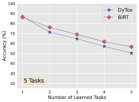
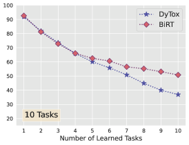
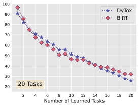
Figure 7: Comparison of performance across learning longer sequence of tasks on CIFAR-100.

Table 4: Quantitative results for the stability-plasticity trade-off in CIFAR-100 for 10 tasks with buffer size 500.

	Plasticity	Stability	Trade-off
DyTox	86.06	29.74	44.16
BiRT - Working Model	66.42	50.52	57.38
BiRT - Semantic Memory	66.08	50.37	57.16

Appendix C Working Principle of DyTox

As mentioned in Section A, we build our proposed approach on top of DyTox framework (Douillard et al.,, 2021), an architecture expansion approach to continual learning with Transformers as the working model. DyTox uses the information about the task id during the training time to learn task-specific classifiers and task tokens. However, no task oracle is used during inference.

DyTox architecture consists of 5 blocks of Self-Attention Blocks (SABs, implemented using ConVit (d’Ascoli et al.,, 2021)) as an encoder to process the input image after the tokenization process. The features predicted by the encoder are then combined with a task token (which is specific to that task) and fed into a Task-Attention Block (TAB), in which the task token attends to the features and extracts the task-specific information. A task-specific classifier projects the processed task token to the number of classes in the task. Thus, the task token and classifier are expanded with respect to every task, while the SAB and TAB blocks are shared between tasks. Furthermore, it employs the copy of the working model at the task boundary as a teacher model to distill the information about past tasks into the working model. DyTox freezes the task tokens and classifier heads of previously learned tasks in order to retain the performance on old tasks.

Appendix D Model Analysis on Other Datasets

We analyze task-wise probability (in Figure 3), stability-plasticity trade-off, and task-recency bias (in Figure 4) on the CIFAR-100 dataset learned for 10 tasks with buffer size 500 in the main text. Here, we show additional results on other datasets (TinyImageNet and ImageNet-100).

Figure 8 illustrates the task-wise accuracy of BiRT vs. DyTox in TinyImageNet. It is evident that BiRT (Semantic Memory) retains more knowledge about past tasks, which in turn helps BiRT (Working Model) achieve better overall performance compared to DyTox. The stability-plasticity trade-off shown in Figure 9 corroborates this conclusion by showing that both the working model and the semantic memory of BiRT have better stability and trade-off values compared to the baseline.

Given that TinyImageNet is one of the challenging benchmarks used in our study, we can see a very high task recency bias in DyTox in Figure 9, suggesting that the model is more likely to predict classes from the last few tasks for samples during inference. The skew toward recent tasks is more pronounced in the TinyImageNet data set compared to CIFAR-100. On the other hand, we can see a more balanced distribution of prediction probabilities in the working model and semantic memory of BiRT.

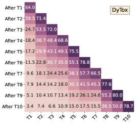
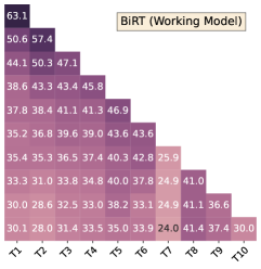
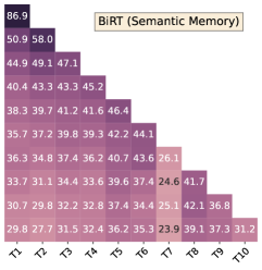
Figure 8: Comparison of task-wise performance after learning every task on TinyImageNet with a buffer size of 500 learned for 10 tasks. The working model achieves better accuracy for the seen tasks after learning 10 tasks compared to DyTox. Semantic memory retains the performance of older tasks better than the baseline and working model.

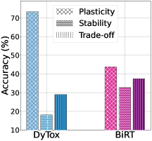
Figure 9: Comparison of the stability-plasticity trade-off (left) and the task-recency bias (right) trained for 10 tasks on TinyImageNet with buffer size 500.

Appendix E Hyperparameters for the Empirical Results

We provide the hyperparameters that we used in our proposed approach for different datasets and tasks in Table 5. Two main hyperparameters in our approach are the decay parameter $\gamma$ that is used to gradually assimilate knowledge into the semantic memory of the working model with frequency $\alpha_{e}$ in Eq. 2 and the weighting parameters $\beta_{1}$ and $\beta_{2}$ in Eq. 6 used to enforce consistency between the working model and the knowledge consolidated in the semantic memory with respect to images from the current task and representations from the buffer memory.

Table 5: Hyperparameters used in BiRT for different datasets and tasks.

Dataset	# of Tasks	Buffer Size	$\gamma$	$\alpha_{e}$	$\beta_{1}$	$\beta_{2}$
CIFAR-100	5	200	0.0005	0.001	0.05	0.01
		500	0.005	0.003	0.05	0.01
	10	200	0.001	0.003	0.05	0.001
		500	0.001	0.003	0.05	0.001
		1000	0.0005	0.0008	0.05	0.01
		2000	0.0002	0.0015	0.05	0.01
	20	200	0.005	0.001	0.05	0.08
		500	0.0005	0.003	0.05	0.1
TinyImageNet	10	500	0.001	0.003	0.05	0.01
		1000	0.01	0.0008	0.01	0.001
		2000	0.0001	0.008	0.01	0.0008
ImageNet-100	10	500	0.0001	0.003	0.05	0.001
		1000	0.0001	0.003	0.05	0.001
		2000	0.01	0.005	0.01	0.001

Table 6: Robustness of BiRT under individual noise in CIFAR-100 dataset.

	BiRT w/o Noise	Supervision Noise	Representation Noise	Attention Noise
Last Acc	45.89	49.64	46.43	49.06
Adv Acc ($\epsilon$=4)	36.52	37.95	36.64	38.39
Adv Acc ($\epsilon$=8)	26.17	26.26	25.64	27.04
Nat Cor Acc	21.82	24.33	21.07	24.42

Appendix F Robustness Analysis with Individual Noise

In order to elucidate the improvements in robustness of BiRT brought about by different noises, we conducted more experiments to ablate the same. As shown in Table 6, overall, every noise proposed in this paper contributes to improving the generalization of stored representations, enabling effective CL in vision transformers. Every noise makes the model less susceptible to adversarial attacks and more robust to natural corruption on the data.

Table 7: Comparison of performance across different noise strengths on CIFAR-100 dataset with buffer size 500.

Supervision Noise		Representation Noise		Attention Noise
Strength (p)	Last Acc	Strength (p)	Last Acc	Strength (p)	Last Acc
0.2	50.90	0.2	51.45	0.2	49.93
0.7	49.85	0.7	49.27	0.8	49.82

Table 8: Comparison of training time taken to learn one task in CIFAR-100 dataset with buffer size 500.

	CIFAR-100	TinyImangeNet	ImageNet-100
DyTox	$\sim$44 mins	$\sim$2 hours 10 mins	$\sim$11 hours 22 mins
BiRT	$\sim$45 mins	$\sim$2 hours 6 mins	$\sim$10 hours 52 mins

Table 9: Comparison between the working model and the semantic memory of BiRT for different datasets and buffer sizes.

Dataset	Buffer Size	Working Model	Semantic Memory
CIFAR-100	500	50.20 $\pm$0.67	50.11 $\pm$0.75
	1000	51.20 $\pm$1.46	51.17 $\pm$1.41
TinyImageNet	500	32.60 $\pm$0.18	32.58 $\pm$0.24
	1000	38.42 $\pm$0.34	38.24 $\pm$0.37
ImageNet-100	500	51.06 $\pm$0.24	50.80 $\pm$0.56
	1000	52.21 $\pm$0.00	51.69$\pm$0.00

Appendix G Sensitivity Analysis to Noise

We control the strength and amount of noise added at different stages of the training process, based on the percentage of samples to which noise is added in each batch. We conducted additional experiments on CIFAR-100 with 10 tasks and a buffer size of 500, varying the percentage of samples to which each noise type is added. The results are shown in Table 7. ‘p’ denotes the percentage of samples to which the corresponding noise is added during the replay of the representation in each batch (batch_size = 128). It is evident that different levels of noise change the last accuracy; however, the performance at different levels of noise reveals that BiRT is not very sensitive to hyperparameters.

Appendix H Training Time Analysis

We conducted an experiment to compare the training time of different CL models considered in this work. The training time on an NVIDIA RTX 2080 Ti for various datasets with buffer size 500 to learn a single task (500 epochs) in CIFAR-100 dataset is enumerated in Table 8. As can be seen, both DyTox and BiRT entail similar training times, indicating that the proposed noise-based approach in BiRT does not increase the training time. In fact, our proposed approach improves generalization performance to a large extent with minimal/no additional computational cost.

Appendix I Analysis on Working Model and Semantic Memory

We compare the performance between DyTox and the BiRT working model in Table 1. However, stochastically assimilating the knowledge learned in the working model into the semantic memory throughout the learning process and at the end of tasks results in a generalized working model with lesser forgetting. We show the last accuracy of the working model and semantic memory for different datasets and buffer sizes in Table 9.

Table 10: Quantitative results for the stability-plasticity analysis of different CL models.

	Plasticity	Stability	Trade-off
DyTox	73.30	18.08	29.01
BiRT	43.73	32.75	37.45

Table 11: Quantitative results of different CL models to different levels of adversarial attacks. Noise in BiRT improves its robustness against adversarial attacks across different epsilon values.

	Average	0	0.25	0.5	1	2	4	8	16	32
DyTox	23.59	35.29	33.35	31.43	29.30	28.26	27.88	19.16	7.03	0.67
BiRT w/o Noise	31.50	47.45	44.74	41.77	38.92	37.54	36.53	26.18	9.54	0.90
BiRT	33.37	50.27	47.32	44.23	41.30	39.79	38.95	27.37	10.12	1.03

Table 12: Quantitative results of different CL models to different levels of natural corruption. Noise in BiRT improves its robustness against natural corruption across different strengths.

	Average	bright.	contrast	defocus	elastic	fog	frost	g_blur	g_noise	glass
DyTox	21.06	26.66	12.38	22.64	21.32	18.57	24.92	21.21	20.99	17.08
BiRT w/o Noise	21.82	28.71	10.99	22.19	21.34	16.07	27.44	20.40	23.41	18.32
BiRT	25.81	32.59	14.19	26.49	25.53	20.04	32.46	24.34	27.17	22.22
	impulse	jpeg	motion	pixelate	saturate	shot	snow	spatter	speckle	zoom
DyTox	18.51	22.69	19.56	24.54	21.60	22.00	21.39	22.43	21.11	20.57
BiRT w/o Noise	19.83	25.23	18.22	24.25	21.36	24.36	25.05	24.57	23.30	19.71
BiRT	22.86	29.71	21.84	28.71	24.68	28.32	29.58	28.67	27.09	23.98

Appendix J Quantitative Results for Model Analysis

Figure 4 in the main text illustrates the stability-plasticity trade-off between DyTox and BiRT. We provide the quantitative results for the same in Table 10. DyTox is more prone to forgetting, whereas BiRT displays a better stability-plasticity trade-off compared to the baseline. We evaluated the robustness of DyTox, BiRT without noise, and BiRT across different strengths of adversarial attacks and natural corruptions. Qualitative results are presented in Figure 5 in the main text. Table 11 and 12 enumerate the quantitative results of the same.

Appendix K Extended Related Works

In addition to the CL methods discussed in the Related Works section in the main text, there is another line of work that pursues the ‘Deep Inversion’ technique to synthesize replay images for old tasks. Deep inversion works by inverting a neural network’s feature extractor to generate synthetic input data that is similar to the original input data. In the context of class incremental learning, deep inversion can be used to generate synthetic data for the new classes that the model needs to learn without requiring access to any real data for those classes (Yin et al.,, 2020; Gao et al.,, 2022; Smith et al.,, 2021). Though this approach alleviates any privacy issues and is more memory-efficient, the model responsible for generating the synthetic data might undergo catastrophic forgetting and this can be exacerbated in long-task sequences.

The theory of a complementary learning system (CLS) posits that the ability to continually acquire and assimilate knowledge over time in the brain is mediated by multiple memory systems (Hassabis et al.,, 2017; Kumaran et al.,, 2016). Inspired by CLS theory, CLS-ER (Arani et al.,, 2021) proposed a dual memory method that maintains multiple semantic memories that interact with episodic memory. On the other hand, FearNet (Kemker and Kanan,, 2017) utilizes a brain-inspired dual-memory system coupled with pseudo rehearsal (Robins,, 1995) in order to efficiently learn new tasks.

Appendix L Limitations

BiRT is a novel continual learning approach that can be applied to various tasks. However, the effectiveness of different levels of noise in BiRT varies in terms of generalization and robustness. The impact of hyperparameters on the effectiveness of different types of noise can also affect accuracy to some extent. However, our empirical results reveal that BiRT is not very sensitive to hyperparameters. BiRT may not be well-suited for datasets with small images (e.g., 32 x 32) since the representations stored in the buffer for such datasets may require more memory compared to storing images. Nonetheless, since real-world datasets typically contain high-resolution images (as in ImageNet-100 and TinyImageNet), BiRT can enable efficient CL in most cases. BiRT does not raise privacy concerns as we do not store personal data, and there are no known bias and fairness issues since we do not use any pretrained weights.

Appendix M Attention Map Analysis

A CL model that is able to preserve the salient regions learned in the first task (when those samples were trained) as learning progresses through the subsequent tasks would provide less catastrophic forgetting (Ebrahimi et al.,, 2021). The [CLS] token in Vision Transformers, which is utilized to infer the class of a sample (Dosovitskiy et al.,, 2020), attends to the salient regions of an image in order to extract rich features pertaining to the task learned by the model. Therefore, it would be beneficial to study the drift in the regions that the model considers to be salient in the image as learning progresses.

Concretely, we study the attention maps calculated by the last Class-Attention block in BiRT for samples in the validation set of the first task as the learning progresses from the first task to the last task. We overlay the attention map as a heatmap (interpolated to the image size) on the image. Figures 10 and 11 show that the BiRT working model preserves the attention map learned in the first task better than DyTox as the training progresses.

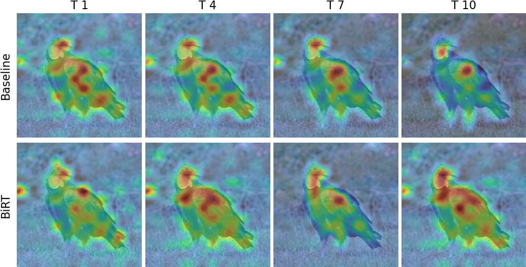
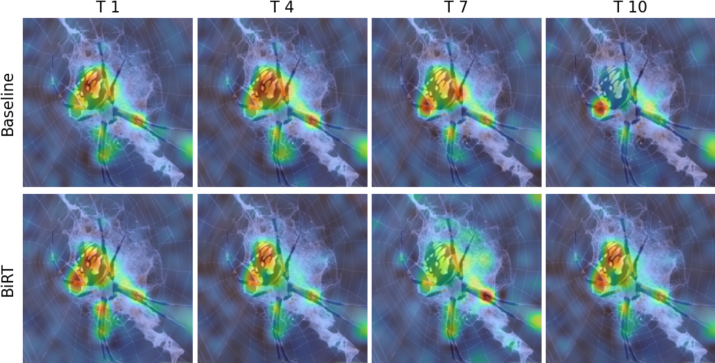
Figure 10: Comparison of attention maps with respect to the class token on the validation set of the first task of ImageNet-100 trained for 10 tasks with buffer size 500. The attention maps are plotted after learning the first, fourth, seventh, and last tasks (red regions correspond to regions with higher attention). BiRT retains the knowledge of salient regions in the image better than DyTox, leading to better predictions and less forgetting.

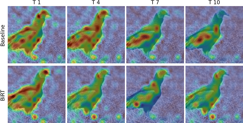
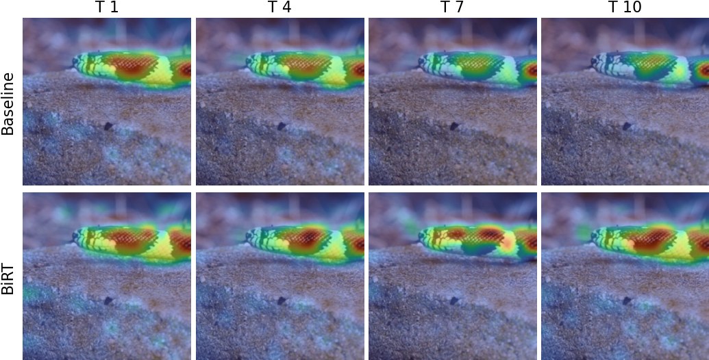
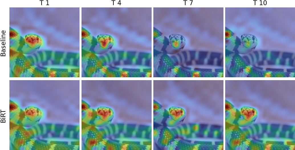
Figure 11: Comparison of attention maps with respect to the class token on the validation set of the first task of ImageNet-100 trained for 10 tasks with buffer size 500. The attention maps are plotted after learning the first, fourth, seventh, and last tasks (red regions correspond to regions with higher attention). BiRT retains the knowledge of salient regions in the image better than DyTox, leading to better predictions and less forgetting.

References

- Aljundi et al., (2017) Aljundi, R., Chakravarty, P., and Tuytelaars, T. (2017). Expert gate: Lifelong learning with a network of experts. In Proceedings of the IEEE Conference on Computer Vision and Pattern Recognition, pages 3366–3375.
- Arani et al., (2021) Arani, E., Sarfraz, F., and Zonooz, B. (2021). Learning fast, learning slow: A general continual learning method based on complementary learning system. In International Conference on Learning Representations.
- Bhat et al., (2022) Bhat, P. S., Zonooz, B., and Arani, E. (2022). Consistency is the key to further mitigating catastrophic forgetting in continual learning. In Conference on Lifelong Learning Agents, pages 1195–1212. PMLR.
- Bhat et al., (2023) Bhat, P. S., Zonooz, B., and Arani, E. (2023). Task-aware information routing from common representation space in lifelong learning. In The Eleventh International Conference on Learning Representations.
- Caccia et al., (2020) Caccia, L., Belilovsky, E., Caccia, M., and Pineau, J. (2020). Online learned continual compression with adaptive quantization modules. In International conference on machine learning, pages 1240–1250. PMLR.
- Chaudhry et al., (2018) Chaudhry, A., Dokania, P. K., Ajanthan, T., and Torr, P. H. (2018). Riemannian walk for incremental learning: Understanding forgetting and intransigence. In Proceedings of the European Conference on Computer Vision (ECCV), pages 532–547.
- Chen et al., (2021) Chen, P., Chen, G., Ye, J., Heng, P.-A., et al. (2021). Noise against noise: stochastic label noise helps combat inherent label noise. In International Conference on Learning Representations.
- d’Ascoli et al., (2021) d’Ascoli, S., Touvron, H., Leavitt, M. L., Morcos, A. S., Biroli, G., and Sagun, L. (2021). Convit: Improving vision transformers with soft convolutional inductive biases. CoRR, abs/2103.10697.
- De Lange et al., (2021) De Lange, M., Aljundi, R., Masana, M., Parisot, S., Jia, X., Leonardis, A., Slabaugh, G., and Tuytelaars, T. (2021). A continual learning survey: Defying forgetting in classification tasks. IEEE transactions on pattern analysis and machine intelligence, 44(7):3366–3385.
- Deng et al., (2009) Deng, J., Dong, W., Socher, R., Li, L.-J., Li, K., and Fei-Fei, L. (2009). Imagenet: A large-scale hierarchical image database. In 2009 IEEE conference on computer vision and pattern recognition, pages 248–255. Ieee.
- Dosovitskiy et al., (2020) Dosovitskiy, A., Beyer, L., Kolesnikov, A., Weissenborn, D., Zhai, X., Unterthiner, T., Dehghani, M., Minderer, M., Heigold, G., Gelly, S., et al. (2020). An image is worth 16x16 words: Transformers for image recognition at scale. arXiv preprint arXiv:2010.11929.
- Douillard and Lesort, (2021) Douillard, A. and Lesort, T. (2021). Continuum: Simple management of complex continual learning scenarios.
- Douillard et al., (2021) Douillard, A., Ramé, A., Couairon, G., and Cord, M. (2021). Dytox: Transformers for continual learning with dynamic token expansion. arXiv preprint arXiv:2111.11326.
- Ebrahimi et al., (2021) Ebrahimi, S., Petryk, S., Gokul, A., Gan, W., Gonzalez, J. E., Rohrbach, M., and Darrell, T. (2021). Remembering for the right reasons: Explanations reduce catastrophic forgetting. Applied AI Letters, 2(4):e44.
- Ermis et al., (2022) Ermis, B., Zappella, G., Wistuba, M., Rawal, A., and Archambeau, C. (2022). Continual learning with transformers for image classification. In Proceedings of the IEEE/CVF Conference on Computer Vision and Pattern Recognition, pages 3774–3781.
- Faisal et al., (2008) Faisal, A. A., Selen, L. P., and Wolpert, D. M. (2008). Noise in the nervous system. Nature reviews neuroscience, 9(4):292–303.
- Farquhar and Gal, (2018) Farquhar, S. and Gal, Y. (2018). Towards robust evaluations of continual learning. arXiv preprint arXiv:1805.09733.
- Fernando et al., (2017) Fernando, C., Banarse, D., Blundell, C., Zwols, Y., Ha, D., Rusu, A. A., Pritzel, A., and Wierstra, D. (2017). Pathnet: Evolution channels gradient descent in super neural networks. arXiv preprint arXiv:1701.08734.
- Gao et al., (2022) Gao, Q., Zhao, C., Ghanem, B., and Zhang, J. (2022). R-dfcil: Relation-guided representation learning for data-free class incremental learning. In Computer Vision–ECCV 2022: 17th European Conference, Tel Aviv, Israel, October 23–27, 2022, Proceedings, Part XXIII, pages 423–439. Springer.
- Hassabis et al., (2017) Hassabis, D., Kumaran, D., Summerfield, C., and Botvinick, M. (2017). Neuroscience-inspired artificial intelligence. Neuron, 95(2):245–258.
- Hayes et al., (2019) Hayes, T. L., Cahill, N. D., and Kanan, C. (2019). Memory efficient experience replay for streaming learning. In 2019 International Conference on Robotics and Automation (ICRA), pages 9769–9776. IEEE.
- Hayes et al., (2020) Hayes, T. L., Kafle, K., Shrestha, R., Acharya, M., and Kanan, C. (2020). Remind your neural network to prevent catastrophic forgetting. In European Conference on Computer Vision, pages 466–483. Springer.
- Hendrycks and Dietterich, (2019) Hendrycks, D. and Dietterich, T. (2019). Benchmarking neural network robustness to common corruptions and perturbations. arXiv preprint arXiv:1903.12261.
- Hinton et al., (2015) Hinton, G., Vinyals, O., and Dean, J. (2015). Distilling the knowledge in a neural network.
- Hou et al., (2019) Hou, S., Pan, X., Loy, C. C., Wang, Z., and Lin, D. (2019). Learning a unified classifier incrementally via rebalancing. In Proceedings of the IEEE/CVF Conference on Computer Vision and Pattern Recognition, pages 831–839.
- Iscen et al., (2020) Iscen, A., Zhang, J., Lazebnik, S., and Schmid, C. (2020). Memory-efficient incremental learning through feature adaptation. In European conference on computer vision, pages 699–715. Springer.
- Jeeveswaran. et al., (2022) Jeeveswaran., K., Kathiresan., S., Varma., A., Magdy., O., Zonooz., B., and Arani., E. (2022). A comprehensive study of vision transformers on dense prediction tasks. In Proceedings of the 17th International Joint Conference on Computer Vision, Imaging and Computer Graphics Theory and Applications - Volume 4: VISAPP,, pages 213–223. INSTICC, SciTePress.
- Ji and Wilson, (2007) Ji, D. and Wilson, M. A. (2007). Coordinated memory replay in the visual cortex and hippocampus during sleep. Nature neuroscience, 10(1):100–107.
- Kemker and Kanan, (2017) Kemker, R. and Kanan, C. (2017). Fearnet: Brain-inspired model for incremental learning. arXiv preprint arXiv:1711.10563.
- Khan et al., (2022) Khan, H., Shah, P. M., Zaidi, S. F. A., et al. (2022). Susceptibility of continual learning against adversarial attacks. arXiv preprint arXiv:2207.05225.
- Kim, (2020) Kim, H. (2020). Torchattacks: A pytorch repository for adversarial attacks. arXiv preprint arXiv:2010.01950.
- Kirkpatrick et al., (2017) Kirkpatrick, J., Pascanu, R., Rabinowitz, N., Veness, J., Desjardins, G., Rusu, A. A., Milan, K., Quan, J., Ramalho, T., Grabska-Barwinska, A., et al. (2017). Overcoming catastrophic forgetting in neural networks. Proceedings of the national academy of sciences, 114(13):3521–3526.
- Krizhevsky et al., (2009) Krizhevsky, A., Hinton, G., et al. (2009). Learning multiple layers of features from tiny images.
- Kudithipudi et al., (2022) Kudithipudi, D., Aguilar-Simon, M., Babb, J., Bazhenov, M., Blackiston, D., Bongard, J., Brna, A. P., Chakravarthi Raja, S., Cheney, N., Clune, J., et al. (2022). Biological underpinnings for lifelong learning machines. Nature Machine Intelligence, 4(3):196–210.
- Kumaran et al., (2016) Kumaran, D., Hassabis, D., and McClelland, J. L. (2016). What learning systems do intelligent agents need? complementary learning systems theory updated. Trends in cognitive sciences, 20(7):512–534.
- Lao et al., (2020) Lao, Q., Jiang, X., Havaei, M., and Bengio, Y. (2020). Continuous domain adaptation with variational domain-agnostic feature replay. arXiv preprint arXiv:2003.04382.
- Le and Yang, (2015) Le, Y. and Yang, X. (2015). Tiny imagenet visual recognition challenge. CS 231N, 7(7):3.
- Li and Hoiem, (2017) Li, Z. and Hoiem, D. (2017). Learning without forgetting. IEEE transactions on pattern analysis and machine intelligence, 40(12):2935–2947.
- Lindsay, (2020) Lindsay, G. W. (2020). Attention in psychology, neuroscience, and machine learning. Frontiers in computational neuroscience, page 29.
- Liu et al., (2022) Liu, S., Zhu, Z., Qu, Q., and You, C. (2022). Robust training under label noise by over-parameterization. In International Conference on Machine Learning, pages 14153–14172. PMLR.
- Liu et al., (2019) Liu, Y., Dolan, R. J., Kurth-Nelson, Z., and Behrens, T. E. (2019). Human replay spontaneously reorganizes experience. Cell, 178(3):640–652.
- Lopez-Paz and Ranzato, (2017) Lopez-Paz, D. and Ranzato, M. (2017). Gradient episodic memory for continual learning. Advances in neural information processing systems, 30.
- Maass, (2014) Maass, W. (2014). Noise as a resource for computation and learning in networks of spiking neurons. Proceedings of the IEEE, 102(5):860–880.
- Mai et al., (2022) Mai, Z., Li, R., Jeong, J., Quispe, D., Kim, H., and Sanner, S. (2022). Online continual learning in image classification: An empirical survey. Neurocomputing, 469:28–51.
- Masana et al., (2020) Masana, M., Liu, X., Twardowski, B., Menta, M., Bagdanov, A. D., and van de Weijer, J. (2020). Class-incremental learning: survey and performance evaluation on image classification. arXiv preprint arXiv:2010.15277.
- McDonnell and Ward, (2011) McDonnell, M. D. and Ward, L. M. (2011). The benefits of noise in neural systems: bridging theory and experiment. Nature Reviews Neuroscience, 12(7):415–425.
- McNaughton and O’Reilly, (1995) McNaughton, B. L. and O’Reilly, R. C. (1995). Why there are complementary learning systems in the hippocampus and neocortex: Insights from the successes and failures of. Psychological Review, 102(3):419–457.
- Parisi et al., (2019) Parisi, G. I., Kemker, R., Part, J. L., Kanan, C., and Wermter, S. (2019). Continual lifelong learning with neural networks: A review. Neural Networks, 113:54–71.
- Pellegrini et al., (2020) Pellegrini, L., Graffieti, G., Lomonaco, V., and Maltoni, D. (2020). Latent replay for real-time continual learning. In 2020 IEEE/RSJ International Conference on Intelligent Robots and Systems (IROS), pages 10203–10209. IEEE.
- Pelosin et al., (2022) Pelosin, F., Jha, S., Torsello, A., Raducanu, B., and van de Weijer, J. (2022). Towards exemplar-free continual learning in vision transformers: an account of attention, functional and weight regularization. In Proceedings of the IEEE/CVF Conference on Computer Vision and Pattern Recognition, pages 3820–3829.
- Peng et al., (2021) Peng, J., Tang, B., Jiang, H., Li, Z., Lei, Y., Lin, T., and Li, H. (2021). Overcoming long-term catastrophic forgetting through adversarial neural pruning and synaptic consolidation. IEEE Transactions on Neural Networks and Learning Systems.
- Raghu et al., (2021) Raghu, M., Unterthiner, T., Kornblith, S., Zhang, C., and Dosovitskiy, A. (2021). Do vision transformers see like convolutional neural networks? Advances in Neural Information Processing Systems, 34.
- Ratcliff, (1990) Ratcliff, R. (1990). Connectionist models of recognition memory: constraints imposed by learning and forgetting functions. Psychological review, 97(2):285.
- Rebuffi et al., (2017) Rebuffi, S.-A., Kolesnikov, A., Sperl, G., and Lampert, C. H. (2017). icarl: Incremental classifier and representation learning. In Proceedings of the IEEE conference on Computer Vision and Pattern Recognition, pages 2001–2010.
- Robins, (1995) Robins, A. (1995). Catastrophic forgetting, rehearsal and pseudorehearsal. Connection Science, 7(2):123–146.
- Rusu et al., (2016) Rusu, A. A., Rabinowitz, N. C., Desjardins, G., Soyer, H., Kirkpatrick, J., Kavukcuoglu, K., Pascanu, R., and Hadsell, R. (2016). Progressive neural networks. arXiv preprint arXiv:1606.04671.
- Sarfraz et al., (2022) Sarfraz, F., Arani, E., and Zonooz, B. (2022). Synergy between synaptic consolidation and experience replay for general continual learning. In Conference on Lifelong Learning Agents, pages 920–936. PMLR.
- Smith et al., (2021) Smith, J., Hsu, Y.-C., Balloch, J., Shen, Y., Jin, H., and Kira, Z. (2021). Always be dreaming: A new approach for data-free class-incremental learning. In Proceedings of the IEEE/CVF International Conference on Computer Vision, pages 9374–9384.
- Srivastava et al., (2014) Srivastava, N., Hinton, G., Krizhevsky, A., Sutskever, I., and Salakhutdinov, R. (2014). Dropout: a simple way to prevent neural networks from overfitting. The journal of machine learning research, 15(1):1929–1958.
- Touvron et al., (2021) Touvron, H., Cord, M., Douze, M., Massa, F., Sablayrolles, A., and Jégou, H. (2021). Training data-efficient image transformers & distillation through attention. In International Conference on Machine Learning, pages 10347–10357. PMLR.
- van de Ven et al., (2020) van de Ven, G. M., Siegelmann, H. T., and Tolias, A. S. (2020). Brain-inspired replay for continual learning with artificial neural networks. Nature communications, 11(1):1–14.
- Van de Ven and Tolias, (2019) Van de Ven, G. M. and Tolias, A. S. (2019). Three scenarios for continual learning. arXiv preprint arXiv:1904.07734.
- Vaswani et al., (2017) Vaswani, A., Shazeer, N., Parmar, N., Uszkoreit, J., Jones, L., Gomez, A. N., Kaiser, Ł., and Polosukhin, I. (2017). Attention is all you need. In Advances in neural information processing systems, pages 5998–6008.
- Verma et al., (2019) Verma, V., Lamb, A., Beckham, C., Najafi, A., Mitliagkas, I., Lopez-Paz, D., and Bengio, Y. (2019). Manifold mixup: Better representations by interpolating hidden states. In International Conference on Machine Learning, pages 6438–6447. PMLR.
- (65) Wang, Z., Liu, L., Duan, Y., Kong, Y., and Tao, D. (2022a). Continual learning with lifelong vision transformer. In Proceedings of the IEEE/CVF Conference on Computer Vision and Pattern Recognition, pages 171–181.
- (66) Wang, Z., Zhang, Z., Ebrahimi, S., Sun, R., Zhang, H., Lee, C.-Y., Ren, X., Su, G., Perot, V., Dy, J., et al. (2022b). Dualprompt: Complementary prompting for rehearsal-free continual learning. arXiv preprint arXiv:2204.04799.
- (67) Wang, Z., Zhang, Z., Lee, C.-Y., Zhang, H., Sun, R., Ren, X., Su, G., Perot, V., Dy, J., and Pfister, T. (2022c). Learning to prompt for continual learning. In Proceedings of the IEEE/CVF Conference on Computer Vision and Pattern Recognition, pages 139–149.
- Yin et al., (2020) Yin, H., Molchanov, P., Alvarez, J. M., Li, Z., Mallya, A., Hoiem, D., Jha, N. K., and Kautz, J. (2020). Dreaming to distill: Data-free knowledge transfer via deepinversion. In Proceedings of the IEEE/CVF Conference on Computer Vision and Pattern Recognition, pages 8715–8724.
- Yoon et al., (2019) Yoon, J., Kim, S., Yang, E., and Hwang, S. J. (2019). Scalable and order-robust continual learning with additive parameter decomposition. arXiv preprint arXiv:1902.09432.
- Yu et al., (2021) Yu, P., Chen, Y., Jin, Y., and Liu, Z. (2021). Improving vision transformers for incremental learning. arXiv preprint arXiv:2112.06103.
- Zenke et al., (2017) Zenke, F., Poole, B., and Ganguli, S. (2017). Continual learning through synaptic intelligence. In International Conference on Machine Learning, pages 3987–3995. PMLR.
- Zhou et al., (2019) Zhou, M., Liu, T., Li, Y., Lin, D., Zhou, E., and Zhao, T. (2019). Toward understanding the importance of noise in training neural networks. In International Conference on Machine Learning, pages 7594–7602. PMLR.