A Closest Point Method for Surface PDEs with Interior Boundary Conditions for Geometry Processing

Abstract.

Many geometry processing techniques require the solution of partial differential equations (PDEs) on surfaces. Such surface PDEs often involve boundary conditions (e.g., Dirichlet or Neumann) prescribed on the surface, at points or curves on its interior or along the geometric (exterior) boundary of an open surface. However, input surfaces can take many forms (e.g., triangle meshes, parametric surfaces, point clouds, level sets, neural implicits, etc.). One must therefore generate a mesh to apply finite element-type techniques or derive specialized discretization procedures for each surface representation.

We propose instead to address such problems through a novel extension of the closest point method (CPM) to handle interior boundary conditions specified at surface points or curves. CPM solves the surface PDE by solving a volumetric PDE defined over the Cartesian embedding space containing the surface; only a closest point function is required to represent the surface. As such, CPM supports surfaces that are open or closed, orientable or not, and of any codimension or even mixed-codimension. To enable support for interior boundary conditions, as required for many geometry processing problems, we develop a method to implicitly partition the embedding space across interior boundaries. CPM’s finite difference and interpolation stencils are adapted to respect this partition while preserving second-order accuracy. Furthermore, an efficient sparse-grid implementation and numerical solver is developed that can scale to tens of millions of degrees of freedom, allowing PDEs to be solved on more complex surfaces. We demonstrate our method’s convergence behaviour on selected model PDEs. Several geometry processing problems are explored: diffusion curves on surfaces, geodesic distance, tangent vector field design, and harmonic map construction. Our proposed approach thus offers a powerful and flexible new tool for a range of geometry processing tasks on general surface representations.

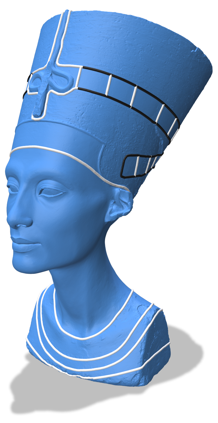
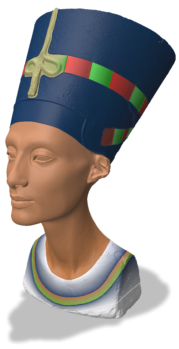
(a) Diffusion Curves

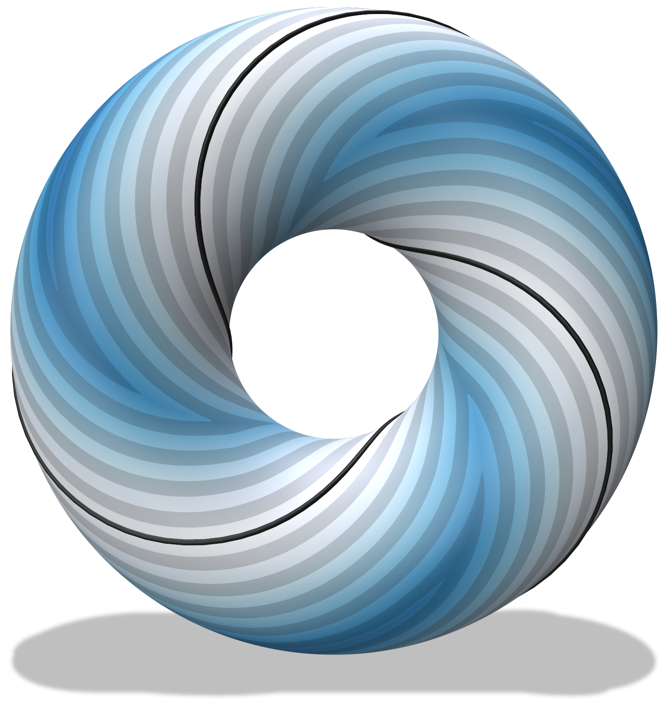
(b) Geodesic Distance

(c) Vector Field Design

Figure 3. We extend the closest point method to support solving surface PDEs with interior boundary conditions. Our method enables the solution of various geometry processing tasks on general surfaces, given only the ability to perform closest point queries. (a) colouring a triangulated surface using diffusion curves. (b) Geodesic distance to a parametric curve (black) on an analytical closest point surface. (c) Vector field design on a Möbius strip, which is an open and nonorientable surface.

1. Introduction

A surface partial differential equation is a partial differential equation (PDE) whose solution is restricted to lie on a surface ${\mathcal{S}}$. Such PDEs arise naturally in many fields, including applied math, mathematical physics, image processing, computer vision, fluid dynamics, and computer graphics. We focus on geometry processing, where a numerical solution is typically sought by approximating the surface as a mesh and discretizing the PDE using finite element or discrete exterior calculus techniques. However, the introduction of a mesh entails some drawbacks. One must perform mesh generation if the input surface is not given as a mesh. The mesh quality also strongly influences the resulting solution. Therefore, remeshing is required if the input mesh is of low quality or inappropriate resolution. Both mesh generation and remeshing are nontrivial tasks. Finally, depending on the chosen method, the discretization of a particular surface PDE can differ significantly from the corresponding discretized PDE on Cartesian domains; further analysis can be needed to derive an appropriate convergent scheme.

A powerful alternative is the use of embedding techniques, which solve the surface problem by embedding it into a surrounding higher-dimensional Cartesian space. The closest point method (CPM) (Ruuth and Merriman, 2008) is an especially attractive instance of this strategy, as it offers a remarkable combination of simplicity and generality. Its simplicity lies in its ability to leverage standard Cartesian numerical methods in the embedding space to solve the desired surface problem, given only a closest point function for the surface. Its generality lies in its support for diverse surface characteristics, surface representations, and surface PDEs.

Requiring only a closest point function allows surfaces that are open or closed, orientable or not, and of any codimension or even mixed codimension. Closest point queries are available for many common surface representations (as recently highlighted by Sawhney and Crane (2020)), and therefore CPM can be applied to meshes, level sets, point clouds, parametric surfaces, constructive solid geometry, neural implicit surfaces, etc. Such generality is appealing given the increasing demand for algorithms that can ingest general “in-the-wild” and high-order geometries ((Hu et al., 2018; Barill et al., 2018; Sawhney and Crane, 2020; Marschner et al., 2021)). Furthermore, the embedding PDE solved on the Cartesian domain is often simply the Cartesian analog of the desired surface PDE. Therefore, prior work has successfully applied CPM to the heat equation, Poisson and screened-Poisson equations, Laplace-Beltrami eigenproblem, biharmonic equation, advection-diffusion and reaction-diffusion equations, Hamilton-Jacobi/level-set equations, Navier-Stokes equation, Cahn-Hilliard equation, computation of ($p$-)harmonic maps, and more.

Yet, despite the desirable properties of CPM and its adoption in applied mathematics, CPM has only infrequently been employed by computer graphics researchers, and almost exclusively for fluid animation (Hong et al., 2010; Auer et al., 2012; Auer and Westermann, 2013; Kim et al., 2013; Morgenroth et al., 2020). In the present work, we demonstrate CPM’s wider potential value for computer graphics problems by extending CPM to handle several applications in geometry processing: diffusion curves on surfaces, geodesic distance, tangent vector field design, and harmonic maps with feature (landmark) points and curves.

However, a crucial limitation of the existing CPM stands in the way of the objective above. CPM supports standard boundary conditions on the geometric (exterior) boundary of an open surface, $\partial{\mathcal{S}}$, but it does not yet support accurate interior boundary conditions (IBCs), i.e., boundary conditions at surface points or curves away from $\partial{\mathcal{S}}$. CPM’s use of the embedding space makes enforcing IBCs nontrivial, but they are vital for the applications above. For example, the curves in diffusion curves or the source points for geodesic distance computation generally lie on the interior of ${\mathcal{S}}$. Therefore, we propose a novel mechanism that enables accurate IBC enforcement in CPM, while retaining its simplicity and generality.

To scale up to surfaces with finer details, we further develop a tailored numerical framework and solver. The computational domain is only required near ${\mathcal{S}}$, so a sparse grid structure is used to improve memory efficiency. The solver also reduces memory consumption by avoiding explicit construction of the full linear system. This is achieved by exploiting a key property of iterative Krylov solvers: explicit construction of the system matrix is not required (in contrast to direct solvers). For iterative Krylov solvers, only the action of the matrix on a given input vector is required (i.e., the matrix-vector product). Thus, we develop a custom preconditioned BiCGSTAB solver for solving the linear system that better utilizes memory. The combination of the sparse grid structure near ${\mathcal{S}}$ and the custom solver allows us to efficiently scale to tens of millions of degrees of freedom. To foster wider adoption of CPM, our code will be released publicly upon acceptance of the paper.

In summary, the key contributions of our work are to:

• introduce a novel treatment of interior boundary conditions for CPM with up to second-order accuracy;

• employ a sparse grid structure and develop a custom solver for memory efficiency, which enables scaling to tens of millions of degrees of freedom; and

• demonstrate the effectiveness of our new CPM scheme for several geometry processing tasks.

2. Related Work

2.1. CPM in Applied Mathematics

CPM was introduced by Ruuth and Merriman (2008), who applied it to diffusion, advection, advection-diffusion, mean curvature flow of curves on surfaces, and reaction-diffusion. They drew inspiration from earlier embedding methods based on level-set surfaces (Bertalmıo et al., 2001; Greer, 2006), while eliminating the restriction to closed surfaces, supporting more general PDEs, and allowing for narrow-banding without loss of convergence order. Subsequently, CPM has been shown to be effective for a wide range of additional PDEs including the screened-Poisson (a.k.a. positive-Helmholtz) equation (Chen and Macdonald, 2015; May et al., 2020), Hamilton-Jacobi equations/level-set equations (Macdonald and Ruuth, 2008), biharmonic equations (Macdonald and Ruuth, 2010), Cahn-Hilliard equation (Gera and Salac, 2017), Navier-Stokes equation (Auer et al., 2012; Yang et al., 2020), construction of ($p$-)harmonic maps (King and Ruuth, 2017), and more. Despite being initially designed for surface PDEs, CPM can additionally be applied to volumetric (codimension-0) problems and surface-to-bulk coupling scenarios (Macdonald et al., 2013). Related closest point mapping approaches have also been used to handle integral equations (Kublik et al., 2013; Kublik and Tsai, 2016; Chen and Tsai, 2017; Chu and Tsai, 2018).

Some prior work on CPM has focused on problems of relevance to geometry processing. For example, Macdonald et al. (2011) computed eigenvalues and eigenfunctions of the Laplace-Beltrami operator via CPM, and the resulting eigenvalues of surfaces were used by Arteaga and Ruuth (2015) to compute the ‘Shape-DNA’ (Reuter et al., 2006) for clustering similar surfaces into groups. Segmentation of data on surfaces was demonstrated by Tian et al. (2009) who adapted the Chan-Vese algorithm common in image processing. Different approaches to compute normals and curvatures were discussed in the appendix of the original CPM paper (Ruuth and Merriman, 2008).

CPM has mostly been used on static surfaces with a uniform grid in the embedding space as the computational domain. However, Petras and Ruuth (2016) combined CPM with a grid-based particle method to solve PDEs on moving surfaces. A mesh-free CPM approach was investigated in (Piret, 2012; Cheung et al., 2015; Petras et al., 2018, 2019, 2022) using radial-basis functions.

The CutFEM family of methods (Burman et al., 2015a) represent another embedding approach but, instead of finite differences, they use a finite element formulation on a non-conforming simplicial embedding mesh. It has been used to solve various surface PDEs (e.g., Laplace-Beltrami (Burman et al., 2015b), convection (Burman et al., 2019).)

2.2. CPM in Computer Graphics

Embedding methods similar to CPM have also been proposed and used in the computer graphics community. Most closely related is the work of Chuang et al. (2009) who estimated the Laplace-Beltrami operator by solving a volumetric grid-based finite element discretization and restricting the solution to the surface. They demonstrated geometry processing applications such as texture back-projection and curvature estimation. They also showed that the observed eigenspectra are much less dependent on the surface triangulation than with standard mesh-based methods. While their approach shares conceptual similarities with CPM, it does not possess the same degree of simplicity or generality as CPM, nor does it support IBCs.

CPM itself has been applied in computer graphics, primarily for fluid animation problems. Hong et al. (2010) used a modified CPM to evolve and control the motion of flame fronts restricted to surfaces. The work of Kim et al. (2013) increased the apparent spatial resolution of an existing volumetric liquid simulation by solving a wave simulation on the liquid surface via CPM. The surface wave equation and Navier-Stokes equations were solved by Auer et al. (2012) with a real-time implementation on the GPU. Auer and Westermann (2013) subsequently extended this method to support deforming surfaces given by a sequence of time-varying triangle meshes (predating the moving surface work of Petras and Ruuth (2016) in computational physics). Morgenroth et al. (2020) employed CPM for one-way coupling between a volumetric fluid simulation and a surface fluid simulation for applications such as oil films spreading on liquid surfaces.

Wang et al. (2020) coupled moving-least-squares approximations on codimension-1 and 2 objects with grid-based approximations for codimension-0 operators in surface-tension driven Navier-Stokes systems. The ability of CPM to handle mixed-codimension objects makes it an ideal candidate for a unified solver.

2.3. Interior Boundary Conditions on Surfaces

Existing numerical methods for surface PDEs support IBCs in various ways depending on the chosen surface representation and method of discretization. In the Dirichlet case, the nearest degrees of freedom (DOFs) to the interior boundary can often simply be assigned the desired Dirichlet value. For example, on a point cloud representation the nearest (interior) points in the cloud can be set to the Dirichlet value, similar to how exterior Dirichlet BCs have been handled in point clouds (Liang and Zhao, 2013). With triangle mesh-based discretizations (finite element, discrete exterior calculus, etc.) one can similarly enforce the Dirichlet condition at the nearest surface vertices to the interior boundaries. However, enforcing the IBC at the nearest DOF is inaccurate if the DOF does not lie exactly on the interior boundary ${\mathcal{C}}$ (i.e., the mesh does not precisely conform to ${\mathcal{C}}$). Specifically, an error of $O(\|{\mathbf{h}}\|)$ is introduced where $\|{\mathbf{h}}\|$ is the distance between the nearest DOF and ${\mathcal{C}}$.

For Dirichlet BCs in CPM, Auer et al. (2012; 2013) fixed all the nearest DOFs in the embedding space within a ball centred around ${\mathcal{C}}$ (considering only the case when ${\mathcal{C}}$ is a point). This again is only first-order accurate, incurring an $O(\Delta x)$ error, where $\Delta x$ is the grid spacing in the embedding space. Enforcing the BC over a ball effectively inflates the boundary region to a wider area of the surface. That is, a circular region of the surface around the point ${\mathcal{C}}$ will be fixed with the prescribed condition. We show in Section 6 that this approach can also be applied to boundary curves, but the observed error is much larger compared to our proposed method. Moreover, it cannot be applied when Dirichlet values differ on each side of ${\mathcal{C}}$.

With a surface triangulation, a more accurate approach is to remesh the surface with constrained Delaunay refinement (possibly with an intrinsic triangulation) so that vertices or edges of the mesh conform to ${\mathcal{C}}$, as discussed for example by Sharp and Crane (2020). However, this necessarily introduces remeshing as an extra preprocess. Another mesh-based approach, which avoids remeshing, is the extended finite element method (Moës et al., 1999; Kaufmann et al., 2009), which uses modified basis functions to enforce non-conforming boundaries or discontinuities.

Most similar to our approach is that of Shi et al. (2007) who enforced Dirichlet IBCs for a surface PDE method based on level-set surfaces. As with CPM, solving surface PDEs with level-set surfaces (Bertalmıo et al., 2001) involves extending the problem to the surrounding embedding space. For such embedding methods, not only does the interior boundary itself need to be considered, but its influence into the embedding space as well. To do so, the approach of Shi et al. (2007) explicitly constructs a triangulation to represent a normal surface ${\mathcal{S}}_{\perp}$ (see (6)) extending outwards from the interior boundary curve ${\mathcal{C}}$ (notably contrasting with the implicit nature of level-sets). They then perform geometric tests to determine if stencils intersect ${\mathcal{S}}_{\perp}$ and modify the discretization locally. We instead introduce a simple triangulation-free approach to determine if stencils cross ${\mathcal{S}}_{\perp}$ that only involves closest points, bypassing explicit construction of ${\mathcal{S}}_{\perp}$. Moreover, such level-set approaches necessarily require a well-defined inside and outside, which makes handling open manifolds, nonorientable surfaces, and manifolds of codimension-two or higher impossible with a single level-set.

Depending on the chosen surface representation and/or discretization, it is also not always obvious how to modify the nearest DOFs to enforce other, non-Dirichlet types of boundary conditions (e.g., Neumann).

Our proposed CPM extension overcomes these and other limitations of the method used by Auer et al. (2012). We demonstrate that our proposed method can easily be extended to second-order, for both Dirichlet and zero-Neumann cases. It can also handle jump discontinuities in Dirichlet values across interior boundary curves. Furthermore, our approach even supports what we call mixed boundary conditions, e.g., Dirichlet on one side and Neumann on the other. Both jump discontinuities and mixed BCs are useful for applications such as diffusion curves (Orzan et al., 2008).

The key attribute of our IBC approach that allows the above flexibility for BC types is the introduction of new DOFs near ${\mathcal{C}}$. This idea shares conceptual similarities with virtual node algorithms (Molino et al., 2004), which have been used for codimension-zero problems (Bedrossian et al., 2010; Hellrung Jr. et al., 2012; Azevedo et al., 2016). It is also similar to the CPM work of  Cheung et al. (2015), who used new DOFs near sharp features of ${\mathcal{S}}$ (albeit with the radial-basis function discretization of CPM).

2.4. Efficiency of CPM

CPM involves constructing a computational domain $\Omega({\mathcal{S}})$ in the embedding space $\mathbb{R}^{d}$ surrounding ${\mathcal{S}}$. Linear systems resulting from the PDE discretization on $\Omega({\mathcal{S}})$ must then be solved. For large linear systems (usually resulting from CPM for problems with $d\geq 3$) memory consumption is dominated by the construction procedure for $\Omega({\mathcal{S}})$. However, computation time is dominated by the linear system solve.

CPM naturally allows $\Omega({\mathcal{S}})$ to occupy only a narrow tubular region of the embedding space near ${\mathcal{S}}$. Therefore, the number of unknowns scales with $\rm{dim}({\mathcal{S}})$ rather than $d$. Note that $\rm{dim}({\mathcal{S}})$ is strictly less than $d$ for surface PDEs. The linear system solve will be faster with fewer unknowns, so it is important that the construction of the computational domain produce a sparse grid, i.e., a grid local to ${\mathcal{S}}$ only. Ruuth and Merriman (2008) used a simple procedure to construct $\Omega({\mathcal{S}})$ that involved storing a uniform grid in a bounding box of ${\mathcal{S}}$ and computing the closest point for every grid point in the bounding box. Finally, an indexing array was used to label which grid points are within a distance $r_{\Omega({\mathcal{S}})}$ of ${\mathcal{S}},$ where $r_{\Omega({\mathcal{S}})}$ is the computational tube-radius (see (4)).

The procedure of Ruuth and Merriman (2008) gives linear systems that scale with $\rm{dim}({\mathcal{S}})$, but memory usage and closest point computation still scale with $d$. Macdonald and Ruuth (2010) used a breadth-first-search (BFS), starting at a grid point near ${\mathcal{S}}$, that allows the number of closest points computed to scale with $\rm{dim}({\mathcal{S}})$. We use a similar BFS when constructing $\Omega({\mathcal{S}})$; see Section 5 for details. However, Macdonald and Ruuth (2010) still required storing the grid in the bounding box of ${\mathcal{S}}$, while we adopt sparse grid structures which achieve efficient memory use by allocating only cells of interest instead of the full grid.

May et al. (2020) overcame memory restrictions due to storing the full bounding-box grid by using domain decomposition to solve the PDE with distributed memory parallelism. The code detailed by May et al. (2022) is publicly available but requires specialized hardware to exploit distributed memory parallelism.

Auer et al. (2012) also used specialized hardware, i.e., their CPM-based fluid simulator was implemented on a GPU. However, they employed a two-level sparse block structure for memory-efficient construction of $\Omega({\mathcal{S}})$ that is also suitable for the CPU. A coarse-level grid in the bounding box of ${\mathcal{S}}$ is used to find blocks of the fine-level grid (used to solve the PDE) that intersect ${\mathcal{S}}$. Thus, the memory usage to construct the fine-level grid $\Omega({\mathcal{S}})$ scales with $\rm{dim}({\mathcal{S}})$, as desired. The coarse-level grid still scales with $d,$ but does not cause memory issues because its resolution is much lower than the fine-level one. We adopt a similar approach for constructing $\Omega({\mathcal{S}})$, although our implementation is purely CPU-based.

There has also been work on efficient linear system solvers for CPM. Chen and Macdonald (2015) developed a geometric multigrid solver for the surface screened-Poisson equation. May et al. (2020, 2022) proposed Schwarz-based domain decomposition solvers and preconditioners for elliptic and parabolic surface PDEs. We implement a custom BiCGSTAB solver (with OpenMP parallelism), as detailed in Section 5.4, that avoids explicit construction of the full linear system. Our solver is more efficient, with respect to memory and computation time (see Section 6.5), compared to Eigen’s SparseLU and BiCGSTAB implementations (Guennebaud et al., 2010). It further avoids the implementation complexities of multigrid or domain decomposition.

3. Closest Point Method and Exterior Boundary Conditions

3.1. Continuous Setting

Consider a surface ${\mathcal{S}}$ embedded in $\mathbb{R}^{d},$ where $d>\rm{dim}({\mathcal{S}})$. The closest point method uses a closest point (CP) surface representation of ${\mathcal{S}}$, which is a mapping from points ${\mathbf{x}}\in\mathbb{R}^{d}$ to points $\text{cp}_{{\mathcal{S}}}({\mathbf{x}})\in{\mathcal{S}}$. The point $\text{cp}_{{\mathcal{S}}}({\mathbf{x}})$ is defined as the closest point on ${\mathcal{S}}$ to ${\mathbf{x}}$ in Euclidean distance, i.e.,

$$\textnormal{\text{cp}}_{{\mathcal{S}}}({\mathbf{x}})=\textnormal{arg}\hskip 0.28436pt\min_{\mathbf{y}\in{\mathcal{S}}}\|{\mathbf{x}}-{\mathbf{y}}\|.$$

A CP surface can be viewed as both an implicit and explicit surface representation: the mapping $\text{cp}_{{\mathcal{S}}}:\mathbb{R}^{d}\rightarrow{\mathcal{S}}$ is an implicit representation, while the closest points themselves give an explicit representation of ${\mathcal{S}}$.

For general ${\mathcal{S}}$, the closest point $\text{cp}_{{\mathcal{S}}}({\mathbf{x}})$ is rarely unique for all ${\mathbf{x}}\in\mathbb{R}^{d}$. For smooth surfaces, however, $\text{cp}_{{\mathcal{S}}}({\mathbf{x}})$ is unique for ${\mathbf{x}}$ in a sufficiently narrow tubular neighbourhood ${\mathcal{N}}({\mathcal{S}})\subseteq\mathbb{R}^{d}$ surrounding ${\mathcal{S}}$ (Marz and Macdonald, 2012). A tubular neighbourhood is defined as

$${\mathcal{N}}({\mathcal{S}})=\left\{{\mathbf{x}}\in\mathbb{R}^{d}\;\Big{|}\;\|{\mathbf{x}}-\text{cp}_{{\mathcal{S}}}({\mathbf{x}})\|<r_{{\mathcal{N}}({\mathcal{S}})}\right\},$$

where $r_{{\mathcal{N}}({\mathcal{S}})}$ is called the tube-radius.

Uniqueness of $\text{cp}_{{\mathcal{S}}}$ is equivalent to requiring ${\mathcal{N}}({\mathcal{S}})\cap\rm{med}({\mathcal{S}})=\emptyset$, since by definition the medial axis of ${\mathcal{S}}$, denoted $\rm{med}({\mathcal{S}}),$ is the subset of $\mathbb{R}^{d}$ that has at least two closest points on ${\mathcal{S}}$. The $\rm{reach}({\mathcal{S}})$ is the minimum distance from ${\mathcal{S}}$ to $\rm{med}({\mathcal{S}})$. Thus, for a uniform radius tube, to ensure uniqueness of $\text{cp}_{{\mathcal{S}}}$ the (maximum) tube-radius is $r_{{\mathcal{N}}({\mathcal{S}})}=\rm{reach}({\mathcal{S}})$. Hence, ${\mathcal{N}}({\mathcal{S}})$ depends on the geometry of ${\mathcal{S}}$ since $\rm{reach}({\mathcal{S}})$ depends on curvatures and bottlenecks (thin regions) of ${\mathcal{S}}$ (see Section 3 of (Aamari et al., 2019)). An adaptive tube-radius for ${\mathcal{N}}({\mathcal{S}})$ could be defined in terms of the local feature size (Amenta and Bern, 1998), but in the present work, only uniform tube-radii are considered for simplicity.

The inset (top) shows an example of a uniform tube ${\mathcal{N}}({\mathcal{S}})$ (gray)

around a 1D surface ${\mathcal{S}}$ (coloured) embedded in $\mathbb{R}^{2}$. To solve surface PDEs with CPM an embedding PDE is constructed on ${\mathcal{N}}({\mathcal{S}})$, whose solution agrees with the solution of the surface PDE at points ${\mathbf{y}}\in{\mathcal{S}}$. Let $\hat{u}({\mathbf{y}}),$ for ${\mathbf{y}}\in{\mathcal{S}},$ and $u({\mathbf{x}})$, for ${\mathbf{x}}\in{\mathcal{N}}({\mathcal{S}}),$ denote the solutions to the surface PDE and embedding PDE, respectively. Fundamentally, CPM is based on extending surface data $\hat{u}$ from ${\mathcal{S}}$ onto ${\mathcal{N}}({\mathcal{S}})$ such that the data is constant in the normal direction of ${\mathcal{S}}$. This task is accomplished using the closest point extension, which is the composition of $\hat{u}$ with $\text{cp}_{{\mathcal{S}}}$, i.e., we take $u({\mathbf{x}})=\hat{u}(\text{cp}_{{\mathcal{S}}}({\mathbf{x}}))$ for all ${\mathbf{x}}\in{\mathcal{N}}({\mathcal{S}})$. In words, the CP extension assigns surface data at the closest point of ${\mathbf{x}}$ to ${\mathbf{x}}$ itself. The inset (bottom) visualizes the data $u\in{\mathcal{N}}({\mathcal{S}})$ resulting from performing this CP extension from surface data $\hat{u}\in{\mathcal{S}}$ (inset, top).

Crucially, Ruuth and Merriman (2008) observed that this extension allows surface differential operators ${\mathcal{L}}_{{\mathcal{S}}}$ on ${\mathcal{S}}$ to be replaced with Cartesian differential operators ${\mathcal{L}}$ on ${\mathcal{N}}({\mathcal{S}})$. Since the function $u$ on ${\mathcal{N}}({\mathcal{S}})$ is constant in the normal direction, $u$ only changes in the tangential direction of ${\mathcal{S}}$. Hence, Cartesian gradients on ${\mathcal{N}}({\mathcal{S}})$ are equivalent to surface gradients for points on the surface. By a similar argument, surface divergence operators can be replaced by Cartesian divergence operators on ${\mathcal{N}}({\mathcal{S}})$. Higher order derivatives are handled by combining these gradient and divergence principles with CP extensions onto ${\mathcal{N}}({\mathcal{S}})$.

Therefore, the embedding PDE to be solved is simply the Cartesian analog of the surface PDE. Throughout this section, we illustrate CPM for solving the surface Poisson equation $\Delta_{{\mathcal{S}}}\hat{u}=\hat{f}$, whose embedding PDE is $\Delta\hat{u}(\text{cp}_{{\mathcal{S}}}({\mathbf{x}}))=\hat{f}(\text{cp}_{{\mathcal{S}}}({\mathbf{x}}))$ or equivalently $\Delta u({\mathbf{x}})=f({\mathbf{x}}).$

3.2. Discrete Setting

In the discrete setting, the computational domain is an irregularly shaped grid $\Omega({\mathcal{S}})\subseteq{\mathcal{N}}({\mathcal{S}})$ with uniform spacing $\Delta x$. The closest point $\text{cp}_{{\mathcal{S}}}({\mathbf{x}}_{i})$ to each grid point ${\mathbf{x}}_{i}\in\Omega({\mathcal{S}})$ is computed and stored. Discrete approximations of the CP extension and the differential operators are needed to solve the embedding PDE. For our example Poisson equation, $\Delta u({\mathbf{x}})=f({\mathbf{x}}),$ we need to approximate the CP extensions $u({\mathbf{x}})=\hat{u}(\text{cp}_{{\mathcal{S}}}({\mathbf{x}}))$ and $f({\mathbf{x}})=\hat{f}(\text{cp}_{{\mathcal{S}}}({\mathbf{x}}))$, as well as the Laplacian $\Delta$. Interpolation is used to approximate the CP extension and finite-differences (FDs) are used for differential operators.

Interpolation is used to perform the CP extension since $\text{cp}_{{\mathcal{S}}}({\mathbf{x}}_{i})$ is generally not a grid point in $\Omega({\mathcal{S}})$. Thus, the surface value $\hat{u}(\text{cp}_{{\mathcal{S}}}({\mathbf{x}}_{i}))$ is approximated by interpolating from discrete values $u_{i}\approx u({\mathbf{x}}_{i})$ stored at grid points ${\mathbf{x}}_{i}\in\Omega({\mathcal{S}})$ surrounding $\text{cp}_{{\mathcal{S}}}({\mathbf{x}}_{i})$. The interpolation order should be chosen such that interpolation error does not dominate the solution. Throughout this paper, we use barycentric-Lagrange interpolation with polynomial degree $p$ (Berrut and Trefethen, 2004). (Surface data given in the surface PDE problem statement, e.g., the function $\hat{f}$ or an initial condition for time-dependent problems, is extended onto $\Omega({\mathcal{S}})$ initially in a different way that depends on the representation of the data. See Section 5 for details.)

More specifically, for a given grid point ${\mathbf{x}}_{k}\in\Omega({\mathcal{S}}),$ we have the following approximation of the closest point extension:

(1) $$\hat{u}(\text{cp}_{{\mathcal{S}}}({\mathbf{x}}_{k}))=u({\mathbf{x}}_{k})\approx\sum_{j\in{\mathcal{I}}_{k}}w_{j}^{k}u_{j},$$

where ${\mathcal{I}}_{k}$ denotes the set of indices corresponding to grid points in the interpolation stencil for the query point $\text{cp}_{{\mathcal{S}}}({\mathbf{x}}_{k})$ and $w_{j}^{k}$ are the barycentric-Lagrange interpolation weights corresponding to each grid point in ${\mathcal{I}}_{k}$.

FD discretizations on $\Omega({\mathcal{S}})$ are used to approximate ${\mathcal{L}}$ as

(2) $${\mathcal{L}}u({\mathbf{x}}_{i})\approx\sum_{k\in{\mathcal{D}}_{i}}l_{k}^{i}u_{k},$$

where ${\mathcal{D}}_{i}$ denotes the set of indices corresponding to grid points in the FD stencil centred at the grid point ${\mathbf{x}}_{i}$. The FD weights are denoted $l_{k}^{i}$ for each ${\mathbf{x}}_{k}$ with $k\in{\mathcal{D}}_{i}$. For example, the common second-order centred-difference for the discrete Laplacian has weights $1/(\Delta x)^{2}$ if $k\neq i$ and $-2d/(\Delta x)^{2}$ if $k=i$.

Given these CP extension and differential operator approximations, the Laplace-Beltrami operator $\Delta_{{\mathcal{S}}}\hat{u}$ is approximated on $\Omega({\mathcal{S}})$ as

(3) $$\Delta_{{\mathcal{S}}}\hat{u}(\text{cp}_{{\mathcal{S}}}({\mathbf{x}}_{i}))\approx\sum_{k\in{\mathcal{D}}_{i}}l_{k}^{i}\left(\sum_{j\in{\mathcal{I}}_{k}}w_{j}^{k}u_{j}\right).$$

Hence, to solve the discrete embedding PDE (for $\Delta_{{\mathcal{S}}}\hat{u}=\hat{f}$) the equation

$$\sum_{k\in{\mathcal{D}}_{i}}l_{k}^{i}\left(\sum_{j\in{\mathcal{I}}_{k}}w_{j}^{k}u_{j}\right)=f_{i},$$

is used to form a linear system to solve for unknowns $u_{i}$ at grid points ${\mathbf{x}}_{i}\in\Omega({\mathcal{S}})$. Finally, the solution to the original surface PDE can be recovered at any ${\mathbf{y}}\in{\mathcal{S}}$ by interpolation as needed. Refer to (Ruuth and Merriman, 2008; Macdonald and Ruuth, 2010; Macdonald et al., 2011) for further background on CPM.

3.2.1. Banding of the Computational Domain

One could use a grid $\Omega({\mathcal{S}})$ that completely fills ${\mathcal{N}}({\mathcal{S}})$, but this choice is inefficient since

only a subset of those points (i.e., those near ${\mathcal{S}}$) affect the numerical solution on the surface. The inset figure shows an example of a grid $\Omega({\mathcal{S}})$ (black) that is smaller than ${\mathcal{N}}({\mathcal{S}})$ (gray) surrounding a surface ${\mathcal{S}}$ (blue). It is only required that all grid points within the interpolation stencil of any surface point have accurate approximations of the differential operators.

Barycentric-Lagrange interpolation uses a hypercube stencil of ${p+1}$ grid points in each dimension. Consider a hyper-cross FD stencil that uses $q$ grid points from the centre of the stencil in each dimension. An upper bound estimate of the computational tube-radius, $r_{\Omega({\mathcal{S}})}$, for the computational domain $\Omega({\mathcal{S}})$ is (Macdonald and Ruuth, 2008; Ruuth and Merriman, 2008)

(4) $$r_{\Omega({\mathcal{S}})}=\Delta x\sqrt{(d-1)\left(\frac{p+1}{2}\right)^{2}+\left(q+\frac{p+1}{2}\right)^{2}}.$$

Therefore, our computational domain $\Omega({\mathcal{S}})$ consists of all grid points ${\mathbf{x}}_{i}$ satisfying $\|{\mathbf{x}}_{i}-\text{cp}_{{\mathcal{S}}}({\mathbf{x}}_{i})\|\leq r_{\Omega({\mathcal{S}})}.$ Explicit construction of $\Omega({\mathcal{S}})$ is discussed in Section 5.

3.3. Exterior Boundary Conditions for Open Surfaces

When the surface ${\mathcal{S}}$ is open (i.e., its geometric boundary $\partial{\mathcal{S}}\neq\emptyset$) some choice of boundary conditions (BC) must usually be imposed on $\partial{\mathcal{S}}$ (e.g., Dirichlet, Neumann, etc.). We will refer to these as exterior boundary conditions. In many applications, however, similar types of boundary conditions may be needed at locations on the interior of ${\mathcal{S}}$, irrespective of ${\mathcal{S}}$ being open or closed. In this case, interior boundary conditions (IBCs) should be enforced on a subset ${\mathcal{C}}\subset{\mathcal{S}}$, which typically consists of points ${\mathcal{C}}$ on a 1D curve ${\mathcal{S}}$, or points and/or curves ${\mathcal{C}}$ on a 2D surface ${\mathcal{S}}$. Our proposed approach for IBCs in Section 4 builds on existing CPM techniques for applying exterior BCs at open surface boundaries, which we review below.

A subset $\Omega(\partial{\mathcal{S}})\subset\Omega({\mathcal{S}})$ of grid points called the boundary subset is used to enforce exterior BCs. $\Omega(\partial{\mathcal{S}})$ consists of all ${\mathbf{x}}_{i}$ satisfying $\text{cp}_{{\mathcal{S}}}({\mathbf{x}}_{i})\in\partial{\mathcal{S}}$, i.e., grid points whose closest surface point is on the boundary of ${\mathcal{S}}$. Equivalently, ${\mathbf{x}}_{i}\in\Omega(\partial{\mathcal{S}})$ has $\text{cp}_{{\mathcal{S}}}({\mathbf{x}}_{i})=\text{cp}_{\partial{\mathcal{S}}}({\mathbf{x}}_{i}),$ where $\text{cp}_{\partial{\mathcal{S}}}$ is the closest point function to $\partial{\mathcal{S}}$:

(5) $$\Omega(\partial{\mathcal{S}})=\big{\{}{\mathbf{x}}_{i}\in\Omega({\mathcal{S}})\;\big{|}\;\|{\mathbf{x}}_{i}-\text{cp}_{\partial{\mathcal{S}}} ({\mathbf{x}}_{i})\|\leq r_{\Omega({\mathcal{S}})},$$

$$\text{cp}_{{\mathcal{S}}}({\mathbf{x}}_{i})=\text{cp}_{\partial{\mathcal{S}}}({\mathbf{x}}_{i})\big{\}}.$$

Geometrically, $\Omega(\partial{\mathcal{S}})$ is a half-tubular region of grid points past $\partial{\mathcal{S}}$. The tube is halved by the surface orthogonal to ${\mathcal{S}}$ at $\partial{\mathcal{S}}$, defined as

(6) $${\mathcal{S}}_{\perp}=\{{\mathbf{x}}\in{\mathcal{N}}({\mathcal{S}})\;|\;{\mathbf{x}}={\mathbf{y}}+t\,{\mathbf{n}}_{{\mathcal{S}}}({\mathbf{y}}),\;{\mathbf{y}}\in\partial{\mathcal{S}},\;|t|\leq r_{{\mathcal{N}}({\mathcal{S}})}\}.$$

The surface normal at ${\mathbf{y}}\in\partial{\mathcal{S}}$ is defined as the limiting normal ${\mathbf{n}}_{{\mathcal{S}}}({\mathbf{y}})=\lim_{\mathbf{z}\rightarrow{\mathbf{y}}}{\mathbf{n}}_{{\mathcal{S}}}(\mathbf{z})$, where $\mathbf{z}\in{\mathcal{S}}$ and ${\mathbf{n}}_{{\mathcal{S}}}({\mathbf{z}})$ is the normal of ${\mathcal{S}}$ at ${\mathbf{z}}$. See Figure 4 for an example of a 1D curve embedded in $\mathbb{R}^{2}$.

Figure 4. The boundary subset $\Omega(\partial{\mathcal{S}})$ (purple points) for a surface ${\mathcal{S}}$ (blue) comprises those grid points in $\Omega({\mathcal{S}})$ (black grid) whose closest point is on the boundary $\partial{\mathcal{S}}$ (white point). The points ${\mathbf{x}}_{i}\in\Omega(\partial{\mathcal{S}})$ are those past the normal surface ${\mathcal{S}}_{\perp}$ based at $\partial{\mathcal{S}}$ (green).

CPM naturally applies first-order homogeneous Neumann BCs, $\nabla_{{\mathcal{S}}}\hat{u}\cdot{\mathbf{n}}_{\partial{\mathcal{S}}}=0$, where ${\mathbf{n}}_{\partial{\mathcal{S}}}$ is the unit conormal of $\partial{\mathcal{S}}$. The conormal is a vector normal to $\partial{\mathcal{S}}$, tangential to ${\mathcal{S}}$, and oriented outward (Dziuk and Elliott, 2007). Therefore, ${\mathbf{n}}_{\partial{\mathcal{S}}}({\mathbf{y}})\neq{\mathbf{n}}_{{\mathcal{S}}}({\mathbf{y}})$ for ${\mathbf{y}}\in\partial{\mathcal{S}},$ but ${\mathbf{n}}_{\partial{\mathcal{S}}}({\mathbf{y}})$ is orthogonal to ${\mathbf{n}}_{{\mathcal{S}}}({\mathbf{y}})$ since ${\mathbf{n}}_{\partial{\mathcal{S}}}({\mathbf{y}})$ is in the tangent space of ${\mathcal{S}}$. The CP extension propagates surface data constant in both ${\mathbf{n}}_{{\mathcal{S}}}$ and ${\mathbf{n}}_{\partial{\mathcal{S}}}$ at $\partial{\mathcal{S}}$, hence, finite differencing across the boundary subset $\Omega(\partial{\mathcal{S}})$ will measure zero conormal derivatives (Ruuth and Merriman, 2008). Therefore, the discretization of the surface differential operator can be used without any changes at ${\mathbf{x}}_{i}\in\Omega(\partial{\mathcal{S}})$.

However, to enforce first-order Dirichlet BCs on $\partial{\mathcal{S}}$, changes must be made to the CP extension step. The prescribed Dirichlet value at the closest point of ${\mathbf{x}}_{i}\in\Omega(\partial{\mathcal{S}})$ is extended to ${\mathbf{x}}_{i}$ (instead of the interpolated value in (1)). That is, the CP extension assigns $u_{i}=\hat{u}(\text{cp}_{{\mathcal{S}}}({\mathbf{x}}_{i}))$ for all ${\mathbf{x}}_{i}\in\Omega(\partial{\mathcal{S}})$, where $\hat{u}(\text{cp}_{{\mathcal{S}}}({\mathbf{x}}_{i}))$ is the prescribed Dirichlet condition at $\text{cp}_{{\mathcal{S}}}({\mathbf{x}}_{i})\in\partial{\mathcal{S}}$. Only this extension procedure changes; the FD discretization is still applied as usual for all exterior BC types and orders.

For improved accuracy, second-order Dirichlet and homogeneous Neumann exterior BCs were introduced by Macdonald et al. (2011) using a simple modification to the closest point function. The closest point function is replaced with

(7) $$\overline{\text{cp}}_{{\mathcal{S}}}({\mathbf{x}})=\text{cp}_{{\mathcal{S}}}(2\text{cp}_{{\mathcal{S}}}({\mathbf{x}})-{\mathbf{x}}).$$

Effectively, rather than finding the closest point, this expression determines a “reflected” point, and returns its closest point instead.

Observe that $\overline{\text{cp}}_{{\mathcal{S}}}$ satisfies $\overline{\text{cp}}_{{\mathcal{S}}}({\mathbf{x}}_{j})=\text{cp}_{{\mathcal{S}}}({\mathbf{x}}_{j})$ if ${\mathbf{x}}_{j}\not\in\Omega(\partial{\mathcal{S}})$

(and $\text{cp}_{{\mathcal{S}}}({\mathbf{x}})$ is unique). Therefore, no change occurs to CPM on the interior of ${\mathcal{S}}$ (see inset, bottom), so we continue to use $\text{cp}_{{\mathcal{S}}}({\mathbf{x}})$ for ${\mathbf{x}}\in\Omega({\mathcal{S}})\setminus\Omega(\partial{\mathcal{S}})$. However, for boundary points ${\mathbf{x}}_{k}\in\Omega(\partial{\mathcal{S}})$, we have $\overline{\text{cp}}_{{\mathcal{S}}}({\mathbf{x}}_{k})\neq\text{cp}_{{\mathcal{S}}}({\mathbf{x}}_{k}),$ since $\overline{\text{cp}}_{{\mathcal{S}}}({\mathbf{x}}_{k})$ is a point on the interior of ${\mathcal{S}}$ while $\text{cp}_{{\mathcal{S}}}({\mathbf{x}}_{k})$ is a point on $\partial{\mathcal{S}}$ (see inset, top). Hence, for a planar surface, $\hat{u}(\overline{\text{cp}}_{{\mathcal{S}}}({\mathbf{x}}_{k}))$ gives the interior mirror value for ${\mathbf{x}}_{k}$. For a general, curved surface this construction gives an approximate mirror value.

Thus, replacing $\text{cp}_{{\mathcal{S}}}$ with $\overline{\text{cp}}_{{\mathcal{S}}}$ will naturally apply second-order homogeneous Neumann exterior BCs: approximate mirror values are extended to ${\mathbf{x}}_{k}\in\Omega(\partial{\mathcal{S}})$, so the effective conormal derivative becomes zero at $\partial{\mathcal{S}}$. This approach generalizes popular methods for codimension-zero problems with embedded boundaries, where mirror values are also assigned to ghost points (see e.g., “second approach” in Section 2.12 of (LeVeque, 2007)). In practice, the only change required is to replace ${\mathcal{I}}_{k}$ and corresponding weights in (1) with those for $\overline{\text{cp}}_{{\mathcal{S}}}({\mathbf{x}}_{k})$.

Second-order Dirichlet exterior BCs similarly generalize their codimension-zero counterparts, e.g., the ghost fluid method (Gibou et al., 2002) that fills ghost point values by linear extrapolation. The CP extension at ${\mathbf{x}}_{k}\in\Omega(\partial{\mathcal{S}})$ becomes $u({\mathbf{x}}_{k})=2\hat{u}(\text{cp}_{{\mathcal{S}}}({\mathbf{x}}_{k}))-u(\overline{\text{cp}}_{{\mathcal{S}}}({\mathbf{x}})),$ where $\hat{u}(\text{cp}_{{\mathcal{S}}}({\mathbf{x}}_{k}))$ is the prescribed Dirichlet value on $\partial{\mathcal{S}}$. Hence, for ${\mathbf{x}}_{k}\in\Omega(\partial{\mathcal{S}})$ we change (1) to

(8) $$u_{k}=2\hat{u}(\text{cp}_{{\mathcal{S}}}({\mathbf{x}}_{k}))-\sum_{j\in\overline{{\mathcal{I}}}_{k}}\overline{w}_{j}^{k}u_{j},$$

where $\overline{{\mathcal{I}}}_{k}$ and $\overline{w}_{j}^{k}$ are the interpolation stencil indices and weights for $\overline{\text{cp}}_{{\mathcal{S}}}({\mathbf{x}}_{k})$, respectively.

Remark that ${\mathcal{S}}$ can have multiple boundaries, so there may be multiple $\Omega(\partial{\mathcal{S}})$ regions where this BC treatment must be applied.

4. Interior Boundary Conditions

As discussed in Section 3, the discrete setting of CPM involves two main operations: interpolation for closest point extensions and FDs for differential operators. Exterior BCs are handled by modifying the CP extension interpolation while keeping the finite differencing the same (Section 3.3). Below we describe our proposed technique to extend CPM with support for interior BCs, which consists of two key changes: adding new degrees of freedom (DOFs) and carefully altering both the interpolation and FD stencils.

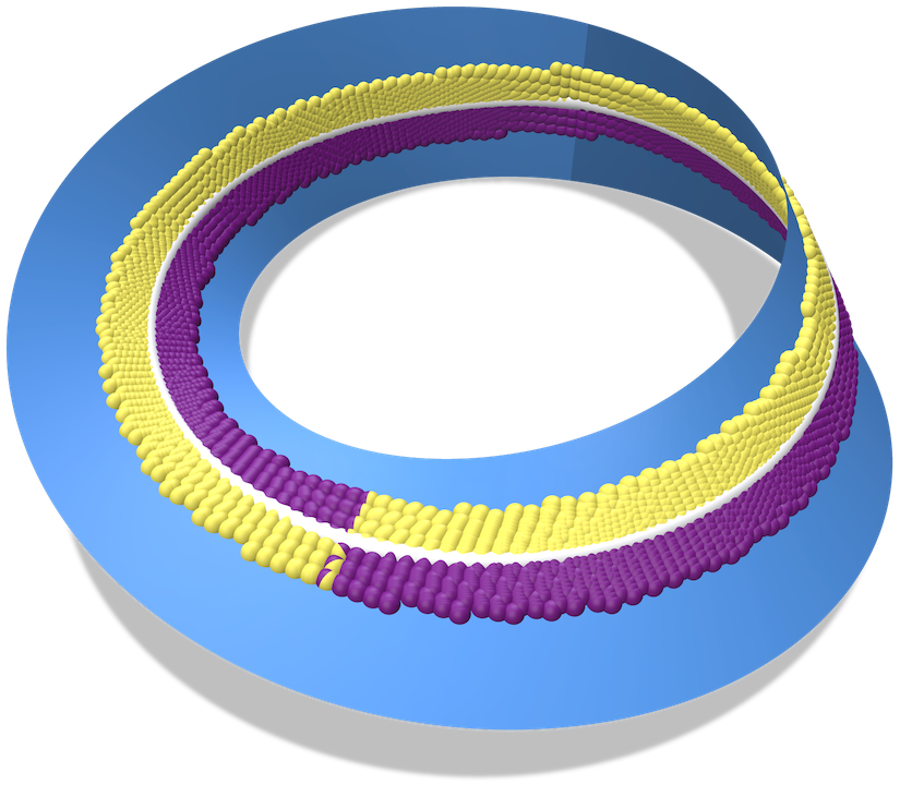
Figure 6. On the left, the (virtual) normal surface ${\mathcal{S}}_{\perp}$ (green) extends perpendicularly outwards from the curve ${\mathcal{C}}$ (white) where IBCs are to be applied on the surface ${\mathcal{S}}$ (blue). On the right, closest points $\text{cp}_{{\mathcal{S}}}({\mathbf{x}}_{i})$ for ${\mathbf{x}}_{i}\in\Omega({\mathcal{C}})$ (yellow and purple points) cannot be globally partitioned into two disjoint sides by a curve ${\mathcal{C}}$ on a nonorientable surface ${\mathcal{S}}$.

Table 1 gives a summary of some of the notation used throughout this paper. Let ${\mathcal{C}}\subset{\mathcal{S}}$ denote the interior region where the BC is to be applied. ${\mathcal{C}}$ can be a point (in 2D or 3D) or an open or closed curve (in 3D). Since CPM is an embedding method we must consider how the effect of ${\mathcal{C}}$ should extend into the embedding space ${\mathcal{N}}({\mathcal{S}})$. Let ${\mathcal{S}}_{\perp}$ denote a (conceptual) surface orthogonal to ${\mathcal{S}}$ along ${\mathcal{C}}$, i.e., analogous to ${\mathcal{S}}_{\perp}$ defined in (6) for the exterior boundary case, but with $\partial{\mathcal{S}}$ replaced by ${\mathcal{C}}$. See Figure 6 (left) for an example curve ${\mathcal{C}}$ on a surface ${\mathcal{S}}$ and its normal surface ${\mathcal{S}}_{\perp}$ at ${\mathcal{C}}$.

Symbol	Description
${\mathcal{S}}$	Surface
${\mathcal{C}}$	Subset of ${\mathcal{S}}$ where IBC is enforced
$\rm{dim({\mathcal{S}})}$	Dimension of surface ${\mathcal{S}}$
$d$	Dimension of embedding space surrounding ${\mathcal{S}}$
$\hat{u}$	Surface function
$u$	Function in embedding space $\mathbb{R}^{d}$
${\mathcal{N}}({\mathcal{S}})$	Tubular neighbourhood surrounding ${\mathcal{S}}$
${\mathbf{n}}_{{\mathcal{S}}}$	Unit surface normal vector
${\mathbf{n}}_{\partial{\mathcal{S}}}$	Unit conormal vector along $\partial{\mathcal{S}}$
${\mathcal{S}}_{\perp}$	Surface orthogonal to ${\mathcal{S}}$ along ${\mathcal{C}}$
$\text{cp}_{{\mathcal{S}}}({\mathbf{x}})$	Closest point in ${\mathcal{S}}$ to ${\mathbf{x}}\in\mathbb{R}^{d}$
$\text{cp}_{{\mathcal{C}}}({\mathbf{x}})$	Closest point in ${\mathcal{C}}$ to ${\mathbf{x}}\in\mathbb{R}^{d}$
$\text{cp}_{{\mathcal{S}}-{\mathcal{C}}}({\mathbf{x}})$	Difference between closest point to ${\mathcal{S}}$ and ${\mathcal{C}}$
$\Omega({\mathcal{S}})$	Irregularly shaped grid surrounding ${\mathcal{S}}$ (subset of ${\mathcal{N}}({\mathcal{S}})$)
$\Omega({\mathcal{C}})$	Interior boundary subset of $\Omega({\mathcal{S}})$
$\Omega(\partial{\mathcal{S}})$	(Exterior) boundary subset of $\Omega({\mathcal{S}})$
$\Omega(\partial{\mathcal{C}})$	Boundary subset of interior boundary subset $\Omega({\mathcal{C}})$
$r_{{\mathcal{N}}({\mathcal{S}})}$	Tube-radius of ${\mathcal{N}}({\mathcal{S}})$
$r_{\Omega({\mathcal{S}})}$	Computational tube-radius
$N_{{\mathcal{S}}}$	Number of grid points in $\Omega({\mathcal{S}})$
$N_{{\mathcal{C}}}$	Number of grid points in $\Omega({\mathcal{C}})$
$J_{{\mathcal{S}}}$	Set of indices for ${\mathbf{x}}_{i}\in\Omega({\mathcal{S}})$
$J_{{\mathcal{C}}}$	Set of indices for ${\mathbf{x}}_{\alpha}\in\Omega({\mathcal{C}})$
$i$	Index in $J_{{\mathcal{S}}}$
$\alpha$	Index in $J_{{\mathcal{C}}}$
${\mathbf{x}}_{i}$	Grid point in $\Omega({\mathcal{S}})$
${\mathbf{x}}_{\alpha}$	Grid point in $\Omega({\mathcal{C}})$

Table 1. A summary of symbols used in this paper.

4.1. Adding Interior Boundary DOFs

Exterior BCs incorporate the BC using grid points ${\mathbf{x}}_{i}\in\Omega(\partial{\mathcal{S}})$ as defined in (5). ${\mathcal{S}}$ does not go through $\Omega(\partial{\mathcal{S}})$ because $\partial{\mathcal{S}}$ is the surface’s (geometric) boundary, i.e., $\Omega(\partial{\mathcal{S}})\cap{\mathcal{S}}=\emptyset$. Therefore, CP extension stencils for ${\mathbf{x}}_{i}\in\Omega(\partial{\mathcal{S}})$ can be safely modified to enforce exterior BCs.

For interior BCs, the situation is more challenging. Similar to $\Omega(\partial{\mathcal{S}})$, a new interior boundary subset $\Omega({\mathcal{C}})\subset\Omega({\mathcal{S}})$ can be defined as

(9) $$\Omega({\mathcal{C}})=\{{\mathbf{x}}_{i}\in\Omega({\mathcal{S}})\;|\;\|{\mathbf{x}}_{i}-\text{cp}_{{\mathcal{C}}}({\mathbf{x}}_{i})\|\leq r_{\Omega({\mathcal{S}})}\},$$

where $\text{cp}_{{\mathcal{C}}}$ is the closest point function of ${\mathcal{C}}$. The subsets $\Omega(\partial{\mathcal{S}})$ and $\Omega({\mathcal{C}})$ are defined in the same way, except $\Omega(\partial{\mathcal{S}})$ has the extra property $\text{cp}_{{\mathcal{S}}}({\mathbf{x}}_{i})=\text{cp}_{\partial{\mathcal{S}}}({\mathbf{x}}_{i})$ for all ${\mathbf{x}}_{i}\in\Omega(\partial{\mathcal{S}})$; i.e., points in the exterior boundary subset have a closest surface point that is also their closest boundary point. Grid points with ${\mathbf{x}}_{i}\in\Omega({\mathcal{C}})$ will in general have $\text{cp}_{{\mathcal{S}}}({\mathbf{x}}_{i})\neq\text{cp}_{{\mathcal{C}}}({\mathbf{x}}_{i}),$ unless the point ${\mathbf{x}}_{i}\in{\mathcal{S}}_{\perp}$.

These facts imply that the intersection of ${\mathcal{S}}$ with $\Omega({\mathcal{C}})$ is not empty. Therefore, we cannot simply repurpose and modify CP extension stencils for ${\mathbf{x}}_{i}\in\Omega({\mathcal{C}})$, since they are needed to solve the surface PDE on ${\mathcal{S}}\setminus{\mathcal{C}}$. A second set of spatially colocated DOFs, called the BC DOFs, must be added at all ${\mathbf{x}}_{i}\in\Omega({\mathcal{C}})$. The BC DOFs allow us to apply similar techniques for interior BCs as was done for exterior BCs.

Specifically, given a computational domain $\Omega({\mathcal{S}})$ of $N_{{\mathcal{S}}}$ grid points and the subset $\Omega({\mathcal{C}})$ of $N_{{\mathcal{C}}}$ grid points, the discrete linear system to be solved will now involve $N_{{\mathcal{S}}}+N_{{\mathcal{C}}}$ DOFs. We order the BC DOFs after the original PDE DOFs. That is, indices in the set $J_{{\mathcal{S}}}=\{j\in\mathbb{N}\;|\;0\leq j<N_{{\mathcal{S}}}\}$ give ${\mathbf{x}}_{j}\in\Omega({\mathcal{S}})$ while indices in the set $J_{{\mathcal{C}}}=\{\alpha\in\mathbb{N}\;|\;N_{{\mathcal{S}}}\leq\alpha<N_{{\mathcal{S}}}+N_{{\mathcal{C}}}\}$ give ${\mathbf{x}}_{\alpha}\in\Omega({\mathcal{C}}).$ Throughout we use Greek letters to denote indices in $J_{{\mathcal{C}}}$ to clearly distinguish from indices in $J_{{\mathcal{S}}}.$ Note that for every BC DOF $\alpha\in J_{{\mathcal{C}}}$ there is a corresponding PDE DOF $j\in J_{{\mathcal{S}}}$ such that ${\mathbf{x}}_{\alpha}={\mathbf{x}}_{j}.$ The key question then becomes: when do we use PDE DOFs versus BC DOFS?

Intuitively, the answer is simple: interpolation and FD stencils (${\mathcal{I}}_{i}$ and ${\mathcal{D}}_{i}$ from (1) and (2)) must only use surface data $\hat{u}$ from the same side of ${\mathcal{S}}_{\perp}$ that the stencil belongs to. Therefore, if a stencil involves surface data on the opposite side of ${\mathcal{S}}_{\perp}$, the IBC must be applied using indices in $J_{{\mathcal{C}}}$, i.e., using the BC DOFs.

Figure 8. A conceptual illustration of our approach to interior boundaries for a point ${\mathcal{C}}$ (white) on a curve ${\mathcal{S}}$ (blue) in $\mathbb{R}^{2}$. Left column: Duplicated BC DOFs are generated in the boundary subset $\Omega({\mathcal{C}})$ around ${\mathcal{C}}$ (thick black grid). Middle column: The normal surface ${\mathcal{S}}_{\perp}$ (green) locally partitions the grid into two sides (yellow, purple). Right column: The modified grid connectivity is illustrated by warping it into $\mathbb{R}^{3}$.

A conceptual illustration of the process for a point ${\mathcal{C}}$ on a circle ${\mathcal{S}}$ embedded in $\mathbb{R}^{2}$ is given in Figure 8. Both BC DOFs and PDE DOFs are present in the region of $\Omega(C)$. The BC DOFs are partitioned into one of two sets depending on which side of ${\mathcal{S}}_{\perp}$ the closest point $\text{cp}_{{\mathcal{S}}}({\mathbf{x}}_{i})$ is on. The original grid $\Omega({\mathcal{S}})$ and duplicated portion $\Omega({\mathcal{C}})$ are cut, and then each half of $\Omega({\mathcal{C}})$ is joined to the opposing side of $\Omega({\mathcal{S}})$.

Figure 9. For two points ${\mathbf{x}}_{1},{\mathbf{x}}_{2}\in{\mathcal{N}}({\mathcal{S}})$, we can determine if the closest points, $\text{cp}_{{\mathcal{S}}}({\mathbf{x}}_{1})$, $\text{cp}_{{\mathcal{S}}}({\mathbf{x}}_{2})$, lie on opposite sides of ${\mathcal{C}}$ based on their orientations relative to the corresponding closest points on ${\mathcal{C}}$, $\text{cp}_{{\mathcal{C}}}({\mathbf{x}}_{1})$, $\text{cp}_{{\mathcal{C}}}({\mathbf{x}}_{2})$.

The same treatment of BCs as in the exterior case is then applied on this nonmanifold grid $\Omega({\mathcal{S}})\cup\Omega({\mathcal{C}})$. That is, the required modifications to the CP extension interpolation stencils in Section 3.3 are applied. Unlike the exerior BC case, however, changes to FD stencils do occur for IBCs since $\Omega({\mathcal{C}})$ and $\Omega({\mathcal{S}})$ are cut and joined to opposite sides of each other.

If the surface ${\mathcal{S}}$ is orientable then this intuitive picture in Figure 8 is an accurate depiction of the necessary grid connectivity. That is, near ${\mathcal{C}}$ we must duplicate DOFs and cut and join opposite pieces of $\Omega({\mathcal{S}})$ and $\Omega({\mathcal{C}})$ to produce regions (similar to $\Omega(\partial{\mathcal{S}})$) where BCs can be imposed. However, if ${\mathcal{S}}$ is nonorientable the closest points $\text{cp}_{{\mathcal{S}}}({\mathbf{x}}_{i})$ for ${\mathbf{x}}_{i}\in\Omega({\mathcal{C}})$ cannot be globally partitioned into two sides. For example, on the Möbius strip in Figure 6 (right), an apparent flip in the partitioning of $\text{cp}_{{\mathcal{S}}}({\mathbf{x}}_{i})$ is unavoidable as one moves along a curve ${\mathcal{C}}$ that loops around the whole strip.

Fortunately, IBCs can still be enforced on nonorientable surfaces because the surface can be oriented locally. The interpolation and FD stencils only perform operations in a small local region of $\Omega({\mathcal{S}})$. Therefore, locally orienting the surface is sufficient to enforce IBCs.

4.2. ${\mathcal{S}}_{\perp}$ Crossing Test

We must keep computation local to each stencil to handle nonorientable surfaces. Therefore, first consider testing if any two closest points of ${\mathbf{x}}_{1},{\mathbf{x}}_{2}\in{\mathcal{N}}({\mathcal{S}})$ are on opposite sides of ${\mathcal{S}}_{\perp}$. A naive approach would be to construct ${\mathcal{S}}_{\perp}$ explicitly, e.g., with a surface triangulation (as was done by Shi et al. (2007)), and then test if the line segment between $\text{cp}_{{\mathcal{S}}}({\mathbf{x}}_{1})$ and $\text{cp}_{{\mathcal{S}}}({\mathbf{x}}_{2})$ intersects the triangulation. However, building an explicit surface is counter to the implicit spirit of CPM.

Determining if $\text{cp}_{{\mathcal{S}}}({\mathbf{x}}_{1})$ and $\text{cp}_{{\mathcal{S}}}({\mathbf{x}}_{2})$ are on opposite sides of ${\mathcal{S}}_{\perp}$ can instead be accomplished based on closest points on ${\mathcal{C}}$. Let $\text{cp}_{{\mathcal{C}}}({\mathbf{x}}_{1})$ and $\text{cp}_{{\mathcal{C}}}({\mathbf{x}}_{2})$ be the closest points to ${\mathbf{x}}_{1}$ and ${\mathbf{x}}_{2}$ on ${\mathcal{C}}$, respectively. Define the vector $\text{cp}_{{\mathcal{S}}-{\mathcal{C}}}({\mathbf{x}})$ as

(10) $$\text{cp}_{{\mathcal{S}}-{\mathcal{C}}}({\mathbf{x}})\equiv\text{cp}_{{\mathcal{S}}}({\mathbf{x}})-\text{cp}_{{\mathcal{C}}}({\mathbf{x}}).$$

Denote the locally-oriented unit normal to ${\mathcal{S}}_{\perp}$ at ${\mathbf{y}}\in{\mathcal{C}}$ as ${\mathbf{n}}_{{\mathcal{S}}_{\perp}}({\mathbf{y}})$. The function

(11) $$F({\mathbf{x}})\equiv\text{cp}_{{\mathcal{S}}-{\mathcal{C}}}({\mathbf{x}})\cdot{\mathbf{n}}_{{\mathcal{S}}_{\perp}}(\text{cp}_{{\mathcal{C}}}({\mathbf{x}}))$$

will have different signs for $F({\mathbf{x}}_{1})$ and $F({\mathbf{x}}_{2})$ if $\text{cp}_{{\mathcal{S}}}({\mathbf{x}}_{1})$ and $\text{cp}_{{\mathcal{S}}}({\mathbf{x}}_{2})$ are on different sides of ${\mathcal{S}}_{\perp}$, or equivalently $F({\mathbf{x}}_{1})F({\mathbf{x}}_{2})<0$. However, this direct test would require computing ${\mathbf{n}}_{{\mathcal{S}}_{\perp}}$ along ${\mathcal{C}}$ and locally orienting that normal vector.

Instead of checking the directions $\text{cp}_{{\mathcal{S}}-{\mathcal{C}}}$ relative to the locally oriented normals ${\mathbf{n}}_{{\mathcal{S}}_{\perp}}$, we can check the directions of $\text{cp}_{{\mathcal{S}}-{\mathcal{C}}}({\mathbf{x}}_{1})$ and $\text{cp}_{{\mathcal{S}}-{\mathcal{C}}}({\mathbf{x}}_{2})$ relative to each other. As illustrated in Figure 9, if $\text{cp}_{{\mathcal{S}}}({\mathbf{x}}_{1})$ and $\text{cp}_{{\mathcal{S}}}({\mathbf{x}}_{2})$ are on opposite sides of ${\mathcal{S}}_{\perp}$ the associated $\text{cp}_{{\mathcal{S}}-{\mathcal{C}}}({\mathbf{x}})$ vectors will point in opposing directions; thus, we can simply check if their dot product is negative:

(12) $$\text{cp}_{{\mathcal{S}}-{\mathcal{C}}}({\mathbf{x}}_{1})\cdot\text{cp}_{{\mathcal{S}}-{\mathcal{C}}}({\mathbf{x}}_{2})<0.$$

In practice, we have found (12) to be sufficient to obtain second-order accuracy in the convergence studies of Section 6 on smooth ${\mathcal{S}}$ and ${\mathcal{C}}$.

When ${\mathbf{x}}$ is close to ${\mathcal{S}}_{\perp}$ the vector $\text{cp}_{{\mathcal{S}}-{\mathcal{C}}}({\mathbf{x}})\approx\mathbf{0},$ which can result in an inaccurate classification of which side $\text{cp}_{{\mathcal{S}}}({\mathbf{x}})$ is on. Therefore, if $\|\text{cp}_{{\mathcal{S}}-{\mathcal{C}}}({\mathbf{x}})\|=\mathcal{O}(\Delta x^{2})$ the point $\text{cp}_{{\mathcal{S}}}({\mathbf{x}})$ is considered to lie on ${\mathcal{C}}$ and can be safely assigned to either side, while maintaining second-order accuracy. In practice, we consider $\text{cp}_{{\mathcal{S}}}({\mathbf{x}})$ to lie on ${\mathcal{C}}$ if $\|\text{cp}_{{\mathcal{S}}-{\mathcal{C}}}({\mathbf{x}})\|<0.1\Delta x^{2}$.

Another benefit of this test (besides not explicitly constructing ${\mathcal{S}}_{\perp}$) is that it can be applied locally in the neighbourhood of a stencil. Therefore, this ${\mathcal{S}}_{\perp}$ crossing test can handle nonorientable surfaces with CPM and IBCs. However, on orientable surfaces one can still globally orient stencils in $\Omega({\mathcal{C}})$ to impose different values or types of IBCs on either side of ${\mathcal{C}}$. For example, different prescribed Dirichlet values on each side of ${\mathcal{C}}$ are useful for vector field design. Mixing Dirichlet and Neumann IBCs on ${\mathcal{C}}$ in this way can also be useful for diffusion curves.

4.3. Stencil Modifications

In this section, we describe how to use the ${\mathcal{S}}_{\perp}$ crossing test to impose IBCs by altering interpolation and FD stencils. The ${\mathcal{S}}_{\perp}$ crossing test (12) allows us to determine if any two points ${\mathbf{x}}_{1},{\mathbf{x}}_{2}\in{\mathcal{N}}({\mathcal{S}})$ have closest points $\text{cp}_{{\mathcal{S}}}({\mathbf{x}}_{1}),\;\text{cp}_{{\mathcal{S}}}({\mathbf{x}}_{2})$ on opposite sides of ${\mathcal{S}}_{\perp}$. Ultimately, we employ this test to determine if the closest points $\text{cp}_{{\mathcal{S}}}({\mathbf{x}}_{j})$ for $j\in{\mathcal{I}}_{i}\;\rm{or}\;{\mathcal{D}}_{i}$ are on the opposite side of ${\mathcal{S}}_{\perp}$ relative to a stencil for ${\mathbf{x}}_{i}$, so the stencil can use the correct PDE vs. BC data.

A stencil is itself assigned to a particular side of ${\mathcal{S}}_{\perp}$ based on the location of an associated point on ${\mathcal{S}}$ that we call the stencil director, denoted ${\mathbf{y}}^{\star}$. For the FD stencil of ${\mathbf{x}}_{i}$ the stencil director is ${\mathbf{y}}^{\star}_{i}=\text{cp}_{{\mathcal{S}}}({\mathbf{x}}_{i})$, since grid data at ${\mathbf{x}}_{i}$ corresponds to surface data at $\text{cp}_{{\mathcal{S}}}({\mathbf{x}}_{i})$. For the interpolation stencil of ${\mathbf{x}}_{i}$ used for the CP extension, the stencil director is the interpolation query point $\text{cp}_{{\mathcal{S}}}({\mathbf{x}}_{i})$, i.e., ${\mathbf{y}}^{\star}_{i}=\text{cp}_{{\mathcal{S}}}({\mathbf{x}}_{i})$.

It is, however, not always the case that ${\mathbf{y}}^{\star}_{i}=\text{cp}_{{\mathcal{S}}}({\mathbf{x}}_{i}).$ Interpolation can also be used to obtain the final solution at any set of surface points. For example, if one desires to transfer the solution to a mesh or a point cloud (e.g., for display or downstream processing), interpolation can be used to obtain the solution on vertices of the mesh or points in the cloud (see Section 5.5). In this case, the stencil director is just the interpolation query point ${\mathbf{y}}^{\star}={\mathbf{y}}_{q}\in{\mathcal{S}}$.

PDE DOF Modifications

The first step to incorporate IBCs is to alter the stencils for the PDE DOFs in $J_{{\mathcal{S}}}$. The computation in both (1) and (2) for $i\in J_{{\mathcal{S}}}$ has the form

$$u_{i}=\sum_{j\in{\mathcal{G}}_{i}}c^{i}_{j}u_{j},$$

where ${\mathcal{G}}_{i}\subset J_{{\mathcal{S}}}$ are indices corresponding to grid points in the stencil for $i$ (i.e., ${\mathcal{G}}_{i}={\mathcal{I}}_{i}$ or ${\mathcal{G}}_{i}={\mathcal{D}}_{i}$) and $c^{i}_{j}$ are corresponding weights.

To incorporate IBCs, the index $j\in{\mathcal{G}}_{i}$ is replaced with its corresponding BC DOF index $\alpha\in J_{{\mathcal{C}}}$ if data at ${\mathbf{x}}_{j}$ comes from the opposite side of ${\mathcal{S}}_{\perp}$. The corresponding stencil weight $c^{i}_{j}$ remains unchanged. Using the ${\mathcal{S}}_{\perp}$ crossing test (12), for all $j\in{\mathcal{G}}_{i}$, we replace $j\in J_{{\mathcal{S}}}$ with its corresponding $\alpha\in J_{{\mathcal{C}}}$ if

(13) $$\text{cp}_{{\mathcal{S}}-{\mathcal{C}}}({\mathbf{y}}^{\star}_{i})\cdot\text{cp}_{{\mathcal{S}}-{\mathcal{C}}}({\mathbf{x}}_{j})<0.$$

If our equations are written in matrix form, these modifications to the PDE DOFs above would change $N_{{\mathcal{S}}}\times N_{{\mathcal{S}}}$ matrices to be size $N_{{\mathcal{S}}}\times(N_{{\mathcal{S}}}+N_{{\mathcal{C}}})$. The next step is to add the BC equations for the BC DOFs in $J_{{\mathcal{C}}}$, resulting in square matrices again of size $(N_{{\mathcal{S}}}+N_{{\mathcal{C}}})\times(N_{{\mathcal{S}}}+N_{{\mathcal{C}}})$.

BC DOF Modifications

Finite-difference stencils are added for the BC DOFs with $\alpha\in J_{{\mathcal{C}}}$ and modified in a similar way to the PDE DOFs above. The same grid connectivity is present in $\Omega({\mathcal{C}})$ as the corresponding portion of $\Omega({\mathcal{S}})$ (except at the boundary of $\Omega({\mathcal{C}})$). Therefore, the same FD stencils on $\Omega({\mathcal{S}})$ are used on $\Omega({\mathcal{C}})$ except with indices $\beta\in J_{{\mathcal{C}}}$ (and indices not present in $\Omega({\mathcal{C}})$, i.e., grid points in $\Omega({\mathcal{S}})$ around the edge of $\Omega({\mathcal{C}})$, are removed). Hence, using the ${\mathcal{S}}_{\perp}$ crossing test (12) for all $\beta\in{\mathcal{D}}_{\alpha}$, the index $\beta\in J_{{\mathcal{C}}}$ is replaced with its corresponding $j\in J_{{\mathcal{S}}}$ if

(14) $$\text{cp}_{{\mathcal{S}}-{\mathcal{C}}}({\mathbf{y}}^{\star}_{\alpha})\cdot\text{cp}_{{\mathcal{S}}-{\mathcal{C}}}({\mathbf{x}}_{\beta})<0.$$

The CP extension BC equations discussed in Section 3.3 for exterior BCs are used on the BC DOFs with $\alpha\in J_{{\mathcal{C}}}$. However, first-order zero-Neumann IBCs are no longer automatically imposed as in Section 3.3. Instead, for first-order zero-Neumann IBCs, the CP extension extends surface data $\hat{u}$ at $\text{cp}_{{\mathcal{C}}}({\mathbf{x}}_{\alpha})$ for ${\mathbf{x}}_{\alpha}\in\Omega({\mathcal{C}})$, i.e.,

$$\hat{u}(\text{cp}_{{\mathcal{C}}}({\mathbf{x}}_{\alpha}))=u({\mathbf{x}}_{\alpha})\approx\sum_{\beta\in{\mathcal{I}}_{\alpha}}w_{\beta}^{\alpha}u_{\beta}.$$

Once again the ${\mathcal{S}}_{\perp}$ crossing test (12) is used to ensure DOFs are used from the correct sides of ${\mathcal{S}}_{\perp}$. In this case, the stencil director (interpolation query point) is ${\mathbf{y}}^{\star}_{\alpha}=\text{cp}_{{\mathcal{C}}}({\mathbf{x}}_{\alpha})$, which gives $\text{cp}_{{\mathcal{S}}-{\mathcal{C}}}({\mathbf{y}}^{\star}_{\alpha})=\mathbf{0}$ since ${\mathbf{y}}^{\star}_{\alpha}$ is on both ${\mathcal{C}}$ and ${\mathcal{S}}$. However, the vector $\text{cp}_{{\mathcal{S}}-{\mathcal{C}}}({\mathbf{y}}^{\star}_{\alpha})=\text{cp}_{{\mathcal{S}}}({\mathbf{x}}_{\alpha})-\text{cp}_{{\mathcal{C}}}({\mathbf{x}}_{\alpha})$ gives the correct direction to define which side of ${\mathcal{S}}_{\perp}$ the interpolation stencil belongs to. Then, for all $\beta\in{\mathcal{I}}_{\alpha}$, we replace $\beta\in J_{{\mathcal{C}}}$ with its corresponding $j\in J_{{\mathcal{S}}}$ if (14) holds.

For second-order zero-Neumann IBCs, the only modification required is to replace $\text{cp}_{{\mathcal{C}}}({\mathbf{x}})$ with

(15) $$\overline{\text{cp}}_{{\mathcal{C}}}({\mathbf{x}})=\text{cp}_{{\mathcal{S}}}(2\text{cp}_{{\mathcal{C}}}({\mathbf{x}})-{\mathbf{x}}).$$

Note that (15) is different from the form used for exterior BCs in (7), as it involves both $\text{cp}_{{\mathcal{S}}}$ and $\text{cp}_{{\mathcal{C}}}$. However, the purpose of this modified closest point function (15) remains the same, i.e., the point $\overline{\text{cp}}_{{\mathcal{C}}}({\mathbf{x}})$ is an approximate mirror location.

The CP extension equations for BC DOFs, with $\alpha\in J_{{\mathcal{C}}},$ to enforce Dirichlet IBCs are analogous to Section 3.3. The prescribed Dirichlet value, $\hat{u}$ on ${\mathcal{C}}$, is extended for first-order Dirichlet IBCs, i.e., $u({\mathbf{x}})=\hat{u}(\text{cp}_{{\mathcal{C}}}({\mathbf{x}}))$ or in the discrete setting $u_{\alpha}=\hat{u}(\text{cp}_{{\mathcal{C}}}({\mathbf{x}}_{\alpha})).$ For second-order Dirichlet IBCs, the extension is $u({\mathbf{x}})=2\hat{u}(\text{cp}_{{\mathcal{C}}}({\mathbf{x}}))-u(\overline{\text{cp}}_{{\mathcal{C}}}({\mathbf{x}})),$ which becomes analogous to (8) in the discrete setting.

4.4. Open Curves ${\mathcal{C}}$ in $\mathbb{R}^{3}$

Past the end points of an open curve ${\mathcal{C}}$ the PDE should be solved without the IBC being enforced. However, the set $\Omega({\mathcal{C}})$ includes half-spherical regions of grid points past the boundary point $\partial{\mathcal{C}}$. These half-spherical regions are analogous to the exterior boundary subsets $\Omega(\partial{\mathcal{S}})$ in Section 3.3 and are defined as

(16) $$\Omega(\partial{\mathcal{C}})=\{{\mathbf{x}}_{\alpha}\in\Omega({\mathcal{C}})\;|\;\text{cp}_{{\mathcal{C}}}({\mathbf{x}}_{\alpha})=\text{cp}_{\partial{\mathcal{C}}}({\mathbf{x}}_{\alpha})\}.$$

We do not perform the modifications of Section 4.3 for points ${\mathbf{x}}_{\alpha}\in\Omega(\partial{\mathcal{C}})$ since this would enforce the IBC where only the PDE should be solved.

4.5. Points ${\mathcal{C}}$ in $\mathbb{R}^{3}$

Remarkably, and unlike for open curves, when ${\mathcal{C}}$ is a point on ${\mathcal{S}}$ embedded in $\mathbb{R}^{3}$ no change to the stencil modification procedure in Section 4.3 is needed. To understand why, consider two simpler options. First, without any boundary treatment whatsoever near ${\mathcal{C}}$ the PDE is solved but the IBC is ignored. Second, a naive first-order treatment simply sets either the nearest grid point or a ball of grid points around ${\mathcal{C}}$ to the Dirichlet value; however, at those grid points the PDE is now ignored. Instead, the grid points near ${\mathcal{C}}$ should be influenced by the IBC at ${\mathcal{C}}$, while also satisfying the PDE.

Under the procedure of Section 4.3, the $\text{cp}_{{\mathcal{S}}-{\mathcal{C}}}$ vectors will point radially outward from the point ${\mathcal{C}}$ (approximately in the tangent space of ${\mathcal{S}}$ at ${\mathcal{C}}$). The ${\mathcal{S}}_{\perp}$ crossing test (12) becomes a half-space test, where the plane $P$ partitioning the space goes through ${\mathcal{C}}$ with its normal given by the stencil director’s vector, $\text{cp}_{{\mathcal{S}}-{\mathcal{C}}}({\mathbf{y}}^{\star}).$ In the stencil for ${\mathbf{y}}^{\star}$, points on the same side of $P$ as ${\mathbf{y}}^{\star}$ are treated as PDE DOFs, while points on the opposite side receive the IBC treatment (either first or second-order as desired). However, the direction of $\text{cp}_{{\mathcal{S}}-{\mathcal{C}}}({\mathbf{y}}^{\star})$, and hence the half-space, changes for each grid point’s stencil (radially around ${\mathcal{C}}$). The $\text{cp}_{{\mathcal{S}}-{\mathcal{C}}}({\mathbf{y}}^{\star})$ changes because the location of $\text{cp}_{{\mathcal{S}}}({\mathbf{y}}^{\star})$ changes with $\text{cp}_{{\mathcal{C}}}({\mathbf{y}}^{\star})$ fixed at ${\mathcal{C}}$. This spinning of $P$ radially around ${\mathcal{C}}$ allows the PDE and the IBC to be enforced simultaneously.

Therefore, for a point ${\mathcal{C}}\in{\mathcal{S}}\subset\mathbb{R}^{3}$, our first-order Dirichlet IBC method acts as an improvement of the approach of Auer et al. (2012), where only points ${\mathbf{x}}_{i}\in\Omega({\mathcal{C}})$ on one side of $P$ (which revolves around ${\mathcal{C}}$) are fixed with the prescribed Dirichlet value. We observe that this reduces the error constant compared to Auer et al. (2012) in convergence studies in Section 6. Furthermore, our approach in Section 4.3 allows us to achieve second-order accuracy, whereas the method of Auer et al. (2012) is restricted to first-order accuracy. Neumann IBCs at a point ${\mathcal{C}}$ are not well-defined since there is no preferred direction conormal to ${\mathcal{C}}$.

4.6. Locally Banding Near ${\mathcal{C}}$

Computation to enforce IBCs should only be performed locally around ${\mathcal{C}}$ for efficiency. The new BC DOFs satisfy this requirement since they are only added at grid points ${\mathbf{x}}_{i}$ within a distance $r_{\Omega({\mathcal{S}})}$ of ${\mathcal{C}}$. This banding of $\Omega({\mathcal{C}})$ is possible for the same reason it is possible to band $\Omega({\mathcal{S}})$ (see Section 3.2.1): grid points are only needed near ${\mathcal{S}}$ and ${\mathcal{C}}$ because accurate approximations of differential operators are only needed at grid points within interpolation stencils.

The use of the ${\mathcal{S}}_{\perp}$ crossing test (12) has been discussed in terms of checking all interpolation and FD stencils in $\Omega({\mathcal{S}})$ and $\Omega({\mathcal{C}})$ above. However, for efficiency, we would like to only check if $\text{cp}_{{\mathcal{S}}}({\mathbf{x}}_{1})$ and $\text{cp}_{{\mathcal{S}}}({\mathbf{x}}_{2})$ are on different sides of ${\mathcal{S}}_{\perp}$ if ${\mathbf{x}}_{1}$ and ${\mathbf{x}}_{2}$ are near ${\mathcal{C}}$. Depending on the geometry of ${\mathcal{S}}$ and ${\mathcal{C}},$ it is not just ${\mathbf{x}}_{i}\in{\Omega({\mathcal{C}})}$ that can have stencils for interpolating at $\text{cp}_{{\mathcal{S}}}({\mathbf{x}}_{i})$ involving grid points that cross ${\mathcal{S}}_{\perp}$.

We therefore check stencils that include grid points ${\mathbf{x}}_{i}\in\Omega({\mathcal{S}})$ with $\|{\mathbf{x}}_{i}-\text{cp}_{{\mathcal{C}}}({\mathbf{x}}_{i})\|<2r_{\Omega({\mathcal{S}})}$ for all the examples in this paper. The closest points $\text{cp}_{{\mathcal{C}}}({\mathbf{x}}_{i})$ are needed to compute $\|{\mathbf{x}}_{i}-\text{cp}_{{\mathcal{C}}}({\mathbf{x}}_{i})\|$. Computation of $\text{cp}_{{\mathcal{C}}}$ for all ${\mathbf{x}}_{i}\in\Omega({\mathcal{S}})$ is avoided using a similar breadth-first search to the one used in the construction of $\Omega({\mathcal{S}})$ (see Algorithm 1 discussed in Section 5).

4.7. Improving Robustness of ${\mathcal{S}}_{\perp}$ Crossing Test

In practice, surfaces with small bumps of high curvature relative to the grid resolution can cause the ${\mathcal{S}}_{\perp}$ crossing test (12) to be inaccurate. For example, the headdress of the Nefertiti mesh in Figure 3 (a) has many small bumps, which causes $\text{cp}_{{\mathcal{S}}-{\mathcal{C}}}$ vectors to be far from orthogonal to ${\mathcal{S}}_{\perp}$ and ${\mathcal{C}}$. The closest points near ${\mathcal{C}}$ are then misclassified as being on the wrong side of ${\mathcal{S}}_{\perp}$.

To make (12) more robust in 3D, we modify the $\text{cp}_{{\mathcal{S}}-{\mathcal{C}}}$ vectors to be orthogonal to ${\mathcal{S}}_{\perp}$ and ${\mathcal{C}}$ before computing the dot product. That is, (12) is used with $\text{cp}_{{\mathcal{S}}-{\mathcal{C}}}({\mathbf{x}})$ replaced by

(17) $$\text{cp}^{\perp}_{{\mathcal{S}}-{\mathcal{C}}}({\mathbf{x}})=\left(\mathbf{I}-{\mathbf{n}}_{{\mathcal{S}}}{\mathbf{n}}_{{\mathcal{S}}}^{T}-{\mathbf{t}}_{{\mathcal{C}}}{\mathbf{t}}_{{\mathcal{C}}}^{T}\right)\text{cp}_{{\mathcal{S}}-{\mathcal{C}}}({\mathbf{x}}),$$

where $\mathbf{I}$ is the identity matrix and ${\mathbf{t}}_{{\mathcal{C}}}$ is the unit tangent vector along ${\mathcal{C}}$. The surface normal ${\mathbf{n}}_{{\mathcal{S}}}$ and tangent ${\mathbf{t}}_{{\mathcal{C}}}$ are evaluated at $\text{cp}_{{\mathcal{C}}}({\mathbf{x}})$. Projecting out the ${\mathbf{n}}_{{\mathcal{S}}}$ and ${\mathbf{t}}_{{\mathcal{C}}}$ components is equivalent to projecting $\text{cp}_{{\mathcal{S}}-{\mathcal{C}}}({\mathbf{x}})$ onto ${\mathbf{n}}_{{\mathcal{S}}_{\perp}}(\text{cp}_{{\mathcal{C}}}({\mathbf{x}})).$ Therefore, the ${\mathcal{S}}_{\perp}$ crossing test (12) becomes equivalent to the direct test that checks if $F({\mathbf{x}}_{1})F({\mathbf{x}}_{2})<0$ (see Section 4.2), but without needing to locally orient ${\mathbf{n}}_{{\mathcal{S}}_{\perp}}$.

The vectors ${\mathbf{n}}_{{\mathcal{S}}}$ and ${\mathbf{t}}_{{\mathcal{C}}}$ must be evaluated at $\text{cp}_{{\mathcal{C}}}({\mathbf{x}})$ since the vector $\text{cp}_{{\mathcal{S}}-{\mathcal{C}}}({\mathbf{x}})$ starts at $\text{cp}_{{\mathcal{C}}}({\mathbf{x}})$ (and goes to $\text{cp}_{{\mathcal{S}}}({\mathbf{x}})$). When ${\mathcal{C}}$ is a single point the tangent direction is undefined, so only the ${\mathbf{n}}_{{\mathcal{S}}}$ component is projected out in this case. It remains to determine ${\mathbf{n}}_{{\mathcal{S}}}$ and ${\mathbf{t}}_{{\mathcal{C}}}$.

For a codimension-one surface ${\mathcal{S}}$ the Jacobian of the closest point function, ${\mathbf{J}}_{\text{cp}_{{\mathcal{S}}}},$ is the projection operator onto the tangent space of ${\mathcal{S}}$ for points on the surface (Marz and Macdonald, 2012; King and Ruuth, 2017). Therefore, the eigenvectors of ${\mathbf{J}}_{\text{cp}_{{\mathcal{S}}}}$ are the surface normal ${\mathbf{n}}_{{\mathcal{S}}}$ and two tangent vectors. However, two arbitrary tangent vectors of ${\mathcal{S}}$ will not suffice; we need the tangent ${\mathbf{t}}_{{\mathcal{C}}}$ along ${\mathcal{C}}$.

A curve ${\mathcal{C}}\in\mathbb{R}^{3}$ has codimension two. The corresponding Jacobian for ${\mathcal{C}}$, ${\mathbf{J}}_{\text{cp}_{{\mathcal{C}}}}$, is likewise equivalent to a projection operator onto the tangent space of ${\mathcal{C}}$ (Kublik and Tsai, 2016). However, the eigenvectors of ${\mathbf{J}}_{\text{cp}_{{\mathcal{C}}}}$ only provide a unique tangent vector ${\mathbf{t}}_{{\mathcal{C}}}$, since the normal and binormal to ${\mathcal{C}}$ can freely rotate around ${\mathbf{t}}_{{\mathcal{C}}}$. Hence, we compute the surface normal ${\mathbf{n}}_{{\mathcal{S}}}$ from the eigendecomposition of ${\mathbf{J}}_{\text{cp}_{{\mathcal{S}}}},$ while ${\mathbf{t}}_{{\mathcal{C}}}$ is computed from the eigendecomposition of ${\mathbf{J}}_{\text{cp}_{{\mathcal{C}}}}.$

Second-order centred FDs in $\Omega({\mathcal{S}})$ are used to compute ${\mathbf{J}}_{\text{cp}_{{\mathcal{S}}}}$. The Jacobian ${\mathbf{J}}_{\text{cp}_{{\mathcal{S}}}}$ is only equivalent to the tangent space projection operator at points on ${\mathcal{S}}$. Therefore, a CP extension must be performed to obtain the projection operator at all points ${\mathbf{x}}_{i}\in\Omega({\mathcal{S}})$, i.e., ${\mathbf{J}}_{\text{cp}_{{\mathcal{S}}}}({\mathbf{x}}_{i})={\mathbf{J}}_{\text{cp}_{{\mathcal{S}}}}(\text{cp}_{{\mathcal{S}}}({\mathbf{x}}_{i}))$. In the discrete setting, the CP extension is computed with the same interpolation discussed in Section 3.2. The Jacobian of $\text{cp}_{{\mathcal{C}}}$ is computed similarly over $\Omega({\mathcal{C}}).$

From the above computation of ${\mathbf{J}}_{\text{cp}_{{\mathcal{S}}}}$ and ${\mathbf{J}}_{\text{cp}_{{\mathcal{C}}}}$, the projection operators are known at points $\text{cp}_{{\mathcal{S}}}({\mathbf{x}}_{i})$ and $\text{cp}_{{\mathcal{C}}}(\mathbf{x}_{i})$, respectively. As such, the ${\mathbf{n}}_{{\mathcal{S}}}$ vectors are not given where they are needed (i.e., at $\text{cp}_{{\mathcal{C}}}({\mathbf{x}}_{i})$). The ${\mathbf{n}}_{{\mathcal{S}}}$ vectors are therefore computed at $\text{cp}_{{\mathcal{C}}}({\mathbf{x}}_{i})$ via barycentric-Lagrange interpolation (with the same degree $p$ polynomials as the CP extension). Interpolating ${\mathbf{n}}_{{\mathcal{S}}}$ requires some care since they are unoriented surface normals. Therefore, when interpolating ${\mathbf{n}}_{{\mathcal{S}}},$ given at points ${\mathbf{x}}_{i}\in\Omega({\mathcal{S}}),$ we locally orient the vectors within each interpolation stencil by negating vectors satisfying

$${\mathbf{n}}_{{\mathcal{S}}}({\mathbf{x}}_{i})\cdot{\mathbf{n}}_{{\mathcal{S}}}(\tilde{{\mathbf{x}}})<0,$$

where $\tilde{{\mathbf{x}}}$ is a single, fixed grid point in the interpolation stencil. Auer et al. (2012) similarly interpolated unoriented normal vectors by locally orienting the vectors, albeit with a different interpolation scheme.

Alternatively, the (unoriented) surface normals could be computed as

$${\mathbf{n}}_{{\mathcal{S}}}({\mathbf{x}})=\frac{{\mathbf{x}}-\text{cp}_{{\mathcal{S}}}({\mathbf{x}})}{\|{\mathbf{x}}-\text{cp}_{{\mathcal{S}}}({\mathbf{x}})\|}.$$

We observed this computation of ${\mathbf{n}}_{{\mathcal{S}}}$ improved robustness somewhat, but still suffered inaccuracies for the ${\mathcal{S}}_{\perp}$ crossing test on some surfaces. By contrast, the FDs and interpolation involved in our computation of ${\mathbf{n}}_{{\mathcal{S}}}$ using ${\mathbf{J}}_{\text{cp}_{{\mathcal{S}}}}$ automatically smooths small, high curvature bumps of the surface, yielding more reliable results in practice.

4.8. A Nearest Point Approach for Dirichlet IBCs

It is also interesting to consider a nearest point approach for handling Dirichlet IBCs at ${\mathcal{C}}$. That is, simply fix the grid points ${\mathbf{x}}_{i}\in\Omega({\mathcal{S}})$ nearest to ${\mathcal{C}}$ with the prescribed Dirichlet value, and remove them as DOFs. This method is similar to techniques discussed in Section 2.3 for other surface representations, e.g., meshes or point clouds. To our knowledge, this approach has not been used with CPM in any previous work.

If ${\mathcal{C}}$ is a point, a single grid point is assigned the Dirichlet value and removed as a DOF. If ${\mathcal{C}}$ is a curve, a set of nearest grid points is obtained (i.e., a raster representation of ${\mathcal{C}}$) and removed as DOFs by assigning Dirichlet values.

This nearest point approach is attractive since new BC DOFs are unnecessary, i.e., $\Omega({\mathcal{C}})$ is not needed. However, it can only be used for Dirichlet IBCs with the same value on both sides of ${\mathcal{C}}$. That is, two-sided Dirichlet IBCs cannot be imposed with the nearest point approach, nor can Neumann IBCs. The nearest point approach is also only first-order accurate since the nearest point can be $\Delta x\sqrt{d}/2$ away from ${\mathcal{C}}$. In Section 6, we observe that the nearest point approach has a better error constant than the method of Auer et al. (2012), but a similar or worse error constant than our first-order IBC approach above (see Figure 13 (d)).

5. Implementation Aspects

5.1. Closest Points and Computational Domain Setup

The method of computing closest points, and its cost, will depend on the underlying surface representation. In Appendix A, we discuss the computation of closest points for some popular representations, including parameterized surfaces, triangulated surfaces, point clouds, signed-distance functions, and more general level-set functions (i.e., implicit surfaces).

To solve PDEs with CPM, the first step is to construct the computational domain $\Omega({\mathcal{S}})$ around ${\mathcal{S}}$. The simplest procedure (Ruuth and Merriman, 2008) involves constructing a grid in a bounding box surrounding ${\mathcal{S}}$, then computing $\text{cp}_{{\mathcal{S}}}$ for each grid point, and finally using only grid points with $\|{\mathbf{x}}_{i}-\text{cp}_{{\mathcal{S}}}({\mathbf{x}}_{i})\|<r_{\Omega({\mathcal{S}})}$ to set up the linear system. This procedure is inefficient as discussed in Section 2.4.

We use a breadth-first search (BFS) procedure to only compute $\text{cp}_{{\mathcal{S}}}$ near $\Omega({\mathcal{S}})$. Memory for the sparse-grid structure is only allocated as needed during the BFS. The BFS can be started from any grid point ${\mathbf{x}}_{0}$ within $r_{\Omega({\mathcal{S}})}$ distance to the surface. The BFS for $\Omega({\mathcal{S}})$ construction is detailed in Algorithm 1. A similar BFS to Algorithm 1 is used to construct $\Omega({\mathcal{C}})$ around ${\mathcal{C}}$.

Algorithm 1 BFS to construct $\Omega({\mathcal{S}})$

Given ${\mathbf{x}}_{0}$ near ${\mathcal{S}}$, i.e., with $\|{\mathbf{x}}_{0}-\text{cp}_{{\mathcal{S}}}({\mathbf{x}}_{0})\|\leq r_{\Omega({\mathcal{S}})}$

Add ${\mathbf{x}}_{0}$ to $\Omega({\mathcal{S}})$ and store $\text{cp}_{{\mathcal{S}}}({\mathbf{x}}_{0})$

Add ${\mathbf{x}}_{0}$ to the queue $Q$

while $Q\neq\emptyset$ do

     Set ${\mathbf{x}}_{\rm{current}}\leftarrow Q$.front()

     for each neighbour ${\mathbf{x}}_{\rm{nbr}}$ of ${\mathbf{x}}_{\rm{current}}$ do

         if ${\mathbf{x}}_{\rm{nbr}}$ has not been visited then

              Compute $\text{cp}_{{\mathcal{S}}}({\mathbf{x}}_{\rm{nbr}})$

              if  $\|{\mathbf{x}}_{\rm{nbr}}-\text{cp}_{{\mathcal{S}}}({\mathbf{x}}_{\rm{nbr}})\|\leq r_{\Omega({\mathcal{S}})}$  then

                  Add ${\mathbf{x}}_{\rm{nbr}}$ to $\Omega({\mathcal{S}})$ and store $\text{cp}_{{\mathcal{S}}}({\mathbf{x}}_{\rm{nbr}})$

                  Add ${\mathbf{x}}_{\rm{nbr}}$ to $Q$

              end if

         end if

     end for

     Pop front of $Q$

end while

The computational tube-radius $r_{\Omega({\mathcal{S}})}$ given by (4) is an upper bound on the grid points needed in $\Omega({\mathcal{S}})$. The stencil set approach to construct $\Omega({\mathcal{S}})$ given by Macdonald and Ruuth (2008, 2010) can reduce the number of DOFs by including only the strictly necessary grid points for interpolation and FD stencils. It was shown by Macdonald and Ruuth (2008) that the reduction in the number of DOFs is between 6-15% for ${\mathcal{S}}$ as the unit sphere. We opted for implementation simplicity over using the stencil set approach due to this low reduction in the number of DOFs.

5.2. Specifying Initial and Boundary Data

Surface PDEs generally involve some given surface data, for initial or boundary conditions, that must first be extended onto $\Omega({\mathcal{S}})$ or $\Omega({\mathcal{C}})$. Examples include $\hat{f}$ in Poisson problems $\Delta_{{\mathcal{S}}}\hat{u}=\hat{f}$, initial conditions $\hat{u}(t=0)$ for time-dependent problems, or Dirichlet IBC values on ${\mathcal{C}}$. The necessary extension procedure depends on the specific representation of the surface and the data, e.g., an analytical function given on a parameterization or discrete data at vertices of a mesh. However, the extension must still be a CP extension: data at $\text{cp}_{{\mathcal{S}}}({\mathbf{x}}_{i})$ (or $\text{cp}_{{\mathcal{C}}}({\mathbf{x}}_{i})$) is assigned to ${\mathbf{x}}_{i}\in\Omega({\mathcal{S}})$ (or $\in\Omega({\mathcal{C}})$).

5.3. Operator Discretization

With the initial data on $\Omega({\mathcal{S}})$ and $\Omega({\mathcal{C}})$, the PDE is then discretized using the equations given in Sections 3 and 4. Matrices $\mathbf{E}$ and $\mathbf{L}$ are constructed for the CP extension and discrete Laplacian, respectively. The standard 7-point discrete Laplacian in $\mathbb{R}^{3}$ (5-point in $\mathbb{R}^{2}$) is used.

In our implementation $\mathbf{E}$ and $\mathbf{L}$ are constructed as discussed by Macdonald and Ruuth (2010). Constructing the (sparse) matrices amounts to storing stencil weights for DOF $i$ in the columns of row $i$. The more numerically stable CPM approximation of the Laplace-Beltrami operator (Macdonald and Ruuth, 2010; Macdonald et al., 2011)

$$\mathbf{M}=\rm{diag}(\mathbf{L})+(\mathbf{L}-\rm{diag}(\mathbf{L}))\mathbf{E},$$

is used instead of $\tilde{\mathbf{M}}=\mathbf{L}\mathbf{E}.$

5.4. Linear Solver

The linear system resulting from CPM could be solved with direct solvers, e.g., Eigen’s SparseLU was used in Section 6.1, but they are only appropriate for smaller linear systems (usually obtained from 1D surfaces embedded in $\mathbb{R}^{2}$). Iterative solvers are preferred for larger linear systems (as noted in (Macdonald and Ruuth, 2010; Chen and Macdonald, 2015)), particularly from problems involving 2D surfaces embedded in $\mathbb{R}^{3}$ or higher. The linear system is non-symmetric due to the closest point extension, therefore Eigen’s BiCGSTAB is an option for larger systems. However, we show in Section 6.5, using Eigen’s BiCGSTAB with the construction of the full matrix system can be too memory intensive.

To efficiently accommodate large-scale problems, we have designed a custom BiCGSTAB solver that is tailored to CPM. Our implementation closely follows the algorithm implemented in Eigen’s BiCGSTAB solver, with subtle differences for memory-efficiency and parallelization.

Specifically, we implemented our solver with the goal of solving linear systems ${\mathbf{A}}{\mathbf{u}}=\mathbf{f}$ with

$${\mathbf{A}}=m{\mathbf{I}}+n\left[\rm{diag}({\mathbf{L}})+\left({\mathbf{L}}-\rm{diag}({\mathbf{L}})\right){\mathbf{E}}\right],$$

where $m\in\{0,1\}$ and $n\in\{1,-\Delta t,-\Delta t/2\}$. This generalized form for ${\mathbf{A}}$ supports the applications described in Sections 6 and 7. For example, setting $m=n=1$ results in the linear system for the screened-Poisson problem described in Section 6.3. The matrices ${\mathbf{E}}$ and ${\mathbf{L}}$ are stored explicitly, as discussed in Section 5.3, and the matrix-vector product ${\mathbf{A}}{\mathbf{u}}$ is computed as follows:

1. Compute $\mathbf{a}={\mathbf{E}}{\mathbf{u}}$.

2. Compute $\mathbf{b}=({\mathbf{L}}-\rm{diag}({\mathbf{L}}))\mathbf{a}$.

3. Compute $\mathbf{a}=\rm{diag}({\mathbf{L}}){\mathbf{u}}$.

4. Return $\mathbf{v}=m{\mathbf{u}}+n\mathbf{a}+n\mathbf{b}$.

OpenMP is used for parallelizing each of the steps over the DOFs.

In addition, iterative Krylov solvers allow for a preconditioner (i.e., approximate inverse operator) for improving convergence of the linear solver. The preconditioner step requires solving the equation $\mathbf{M}{\mathbf{z}}=\boldsymbol{r}$, where $\mathbf{M}$ is an approximation to ${\mathbf{A}}$ and $\boldsymbol{r}$ is the residual vector. Depending on the particular problem, we either use a diagonal preconditioner or a damped-Jacobi preconditioner. Computing the diagonal entries of ${\mathbf{A}}$ would require extra computations since the full matrix is not constructed. In practice, however, we found that the diagonal values of $m{\mathbf{I}}+n\rm{diag}({\mathbf{L}})$ are a good enough approximation. (In our experiments, we have verified that the infinity norm of the error matches the result produced by Eigen’s solver.) For damped-Jacobi preconditioning, the iteration ${\mathbf{u}}\leftarrow{\mathbf{u}}+\omega\rm{diag}({\mathbf{L}})^{-1}\boldsymbol{r}$ is applied for a fixed number of iterations with $\omega=2/3$.

5.5. Visualization

Visualization of the solution can be obtained in multiple ways. Demir and Westermann (2015) proposed a direct raycasting approach based on the closest points $\text{cp}_{{\mathcal{S}}}({\mathbf{x}}_{i})$ for ${\mathbf{x}}_{i}\in\Omega({\mathcal{S}})$. The set of $\text{cp}_{{\mathcal{S}}}({\mathbf{x}}_{i})$ can also be considered a point cloud and visualized as such. Lastly, interpolation allows the solution to be transferred to any explicit representation, e.g., triangle mesh, point cloud, etc.

For convenience, we visualize the surface solution at points $\text{cp}_{{\mathcal{S}}}({\mathbf{x}}_{i})$ (e.g., Figure 24) or interpolate onto a triangulation. If the given surface ${\mathcal{S}}$ is provided as a triangulation we use it; if a surface can be described by a parameterization, we connect evenly spaced points in the parameter space to create a triangulation. Both point clouds and triangulations are visualized using polyscope (Sharp et al., 2019b).

6. Convergence Studies

We begin our evaluation by verifying that our proposed IBC schemes achieve the expected convergence orders on various analytical problems. We also compare our approach with the existing CPM approach of Auer et al. (2012), as well as a mesh-based method. Furthermore, a comparison between our partially matrix-free solver and Eigen’s SparseLU and BiCGSTAB implementations (Guennebaud et al., 2010) is given. Throughout the rest of the paper, the hat symbol has been dropped from surface functions (e.g., $\hat{u}$), since it is apparent from the context.

6.1. Poisson Equation with Discontinuous Solution

Consider the Poisson equation

$$-\frac{\partial^{2}u}{\partial\theta^{2}} =2\cos(\theta-\theta_{{\mathcal{C}}}),$$

$$u(\theta_{{\mathcal{C}}}^{-}) =2,$$

$$u(\theta_{{\mathcal{C}}}^{+}) =22,$$

on the unit circle parameterized by $\theta$. The right-hand-side expression is found by differentiating the exact solution

$$u(\theta)=2\cos(\theta-\theta_{{\mathcal{C}}})+\frac{10}{\pi}(\theta-\theta_{{\mathcal{C}}}),$$

where $\theta_{{\mathcal{C}}}$ is the location of the Dirichlet IBC. The Dirichlet IBC is two-sided and thus discontinuous at the point $\theta_{{\mathcal{C}}}$, with $u=2$ as $\theta\rightarrow\theta_{{\mathcal{C}}}^{-}$ and $u=22$ as $\theta\rightarrow\theta_{{\mathcal{C}}}^{+}$. We use $\theta_{{\mathcal{C}}}=1.022\pi$; no grid points coincide with the IBC location.

Eigen’s SparseLU is used to solve the linear system for this problem on the circle embedded in $\mathbb{R}^{2}$. Figure 10 (a) shows that the first and second-order IBCs discussed in Section 4 achieve the expected convergence rates. The nearest point approach (Section 4.8) and the method of Auer et al. (2012) cannot handle discontinuous IBCs.

Figure 10. Convergence studies and associated geometries for the model problems in Sections  6.1-6.3. The plots show results for our CPM approach using first (blue) and second (orange) order IBCs, along with lines of slopes 1 (gray, dashed) and 2 (gray, dotted).

6.2. Heat Equation

CPM can also be applied to time-dependent problems. Consider the heat equation

(18) $$\frac{\partial u}{\partial t}=\Delta_{{\mathcal{S}}}u,\quad\rm{with}\quad\begin{cases}u=g,\;\rm{or}\\ \nabla_{{\mathcal{S}}}u\cdot{\mathbf{b}}_{{\mathcal{C}}}=0,\end{cases}\rm{on}\;{\mathcal{C}},$$

where ${\mathbf{b}}_{{\mathcal{C}}}$ is the binormal direction to ${\mathcal{C}}$ that is also in the tangent plane of ${\mathcal{S}},$ i.e., ${\mathbf{b}}_{{\mathcal{C}}}={\mathbf{n}}_{{\mathcal{S}}}\times{\mathbf{t}}_{{\mathcal{C}}}$ (see Section 4.7). If imposing the Dirichlet IBC, the exact solution, $g,$ is used as the prescribed function on ${\mathcal{C}}$. Here we solve the heat equation on the unit sphere with the exact solution

$$g(\theta,\phi,t)=e^{-2t}\cos(\phi),$$

where $\theta$ is the azimuthal angle and $\phi$ is the polar angle. The IBC is imposed with ${\mathcal{C}}$ as a circle defined by the intersection of a plane with ${\mathcal{S}}$. The initial condition is taken as $g(\theta,\phi,0)=\cos(\phi).$

Crank-Nicolson time-stepping (LeVeque, 2007) (i.e., trapezoidal rule) is used with $\Delta t=0.1\Delta x$ until time $t=0.1.$ Figure 10 (b) and (c) show convergence studies for (18) with Dirichlet and zero-Neumann IBCs imposed, respectively. The expected order of accuracy for first and second-order IBCs is achieved for both the Dirichlet and zero-Neumann cases. Recall that the nearest point approach and the method of Auer et al. (2012) cannot handle Neumann IBCs.

6.3. Screened-Poisson Equation

Exact solutions for surface PDEs can also be derived on more complex surfaces defined as level-sets. Consider the screened-Poisson problem in Section 4.6.5 of (Chen and Macdonald, 2015), which was inspired by an example by Dziuk (1988). The surface is defined as ${\mathcal{S}}=\{{\mathbf{x}}\in\mathbb{R}^{3}\;|\;(x_{1}-x_{3}^{2})^{2}+x_{2}^{2}+x_{3}^{2}=1\},$ which we refer to as the Dziuk surface.

The screened-Poisson equation we solve is

(19) $$-\Delta_{{\mathcal{S}}}u+u =f,$$

$$\nabla_{{\mathcal{S}}}u\cdot{\mathbf{b}}_{{\mathcal{C}}} =0,$$

with exact solution $u({\mathbf{x}})=x_{1}x_{2}.$ Even though the solution is simple, the function $f$ is quite complicated; we derived it by symbolic differentiation using the formulas in (Chen and Macdonald, 2015; Dziuk, 1988).

The zero-Neumann IBC of (19) is satisfied on the intersection of ${\mathcal{S}}$ with the $x_{1}x_{2}$-plane. From the definition of ${\mathcal{S}}$, this intersection is the unit circle in the $x_{1}x_{2}$-plane. Figure 10 (d) and (e) show convergence studies imposing the zero-Neumann IBC on the full circle (closed curve) and the arc with $\theta\in[-\frac{3\pi}{4},\frac{\pi}{4}]$ (open curve), respectively. The expected order of accuracy is observed for the implementations of first and second-order IBCs.

6.4. Comparison of CPM approaches and a Mesh-Based Method

CPM is principally designed to solve problems on general surfaces given by their closest point functions. The closest point function can be thought of as a black box allowing many surface representations to be handled in a unified framework. Hence, one should not expect CPM to universally surpass specially tailored and well-studied approaches for particular surface representations, such as finite elements on (quality) triangle meshes. Nevertheless, mesh-based schemes provide a useful point of reference for our evaluation. CPM retains some advantages even in that setting, such as mesh-independent behaviour.

Therefore, we compare the various CPM approaches to the standard cotangent Laplacian (Pinkall and Polthier, 1993; Dziuk, 1988) that approximates the Laplace-Beltrami operator on a triangulation of the surface. We use the implementation from geometry-central (Sharp et al., 2019a), adapted slightly to include IBCs. The Poisson equation $-\Delta_{{\mathcal{S}}}u=f$ is solved on the Dziuk surface defined in Section 6.3. The same exact solution $u({\mathbf{x}})=x_{1}x_{2}$ is used, but Dirichlet IBCs are imposed using this exact solution.

“Good” and “bad” triangulations, $\mathcal{T}_{g}$ and $\mathcal{T}_{b}$ respectively, of the Dziuk surface, are used to illustrate the dependence of the mesh-based method on triangulation quality (Figure 12). Both triangulations are constructed starting from six vertices on ${\mathcal{S}}$ as in (Dziuk, 1988). An initial round of 1:4 subdivision is performed by adding new vertices along each edge, at the midpoint for $\mathcal{T}_{g}$ and at the 20% position for $\mathcal{T}_{b}$, to induce skinnier triangles in the latter. The new vertices are projected to their closest points on ${\mathcal{S}}$.

Evaluations under refinement for the mesh-based method are performed starting with the above first-level $\mathcal{T}_{g}$ and $\mathcal{T}_{b}$. We refine with uniform 1:4 subdivision, for both $\mathcal{T}_{g}$ and $\mathcal{T}_{b},$ by adding new vertices at midpoints of edges and then projecting them onto ${\mathcal{S}}$ (see Figure 12). Delaunay edge flips are also performed to improve the quality of $\mathcal{T}_{g}$ at each refinement level.

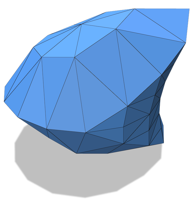
$\mathcal{T}_{g}$

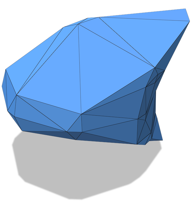
$\mathcal{T}_{b}$

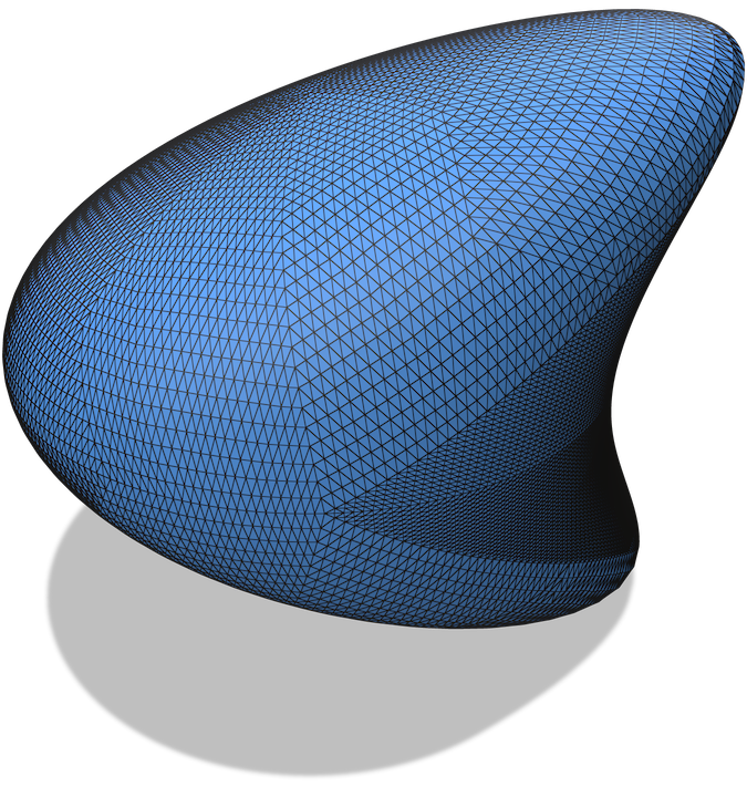
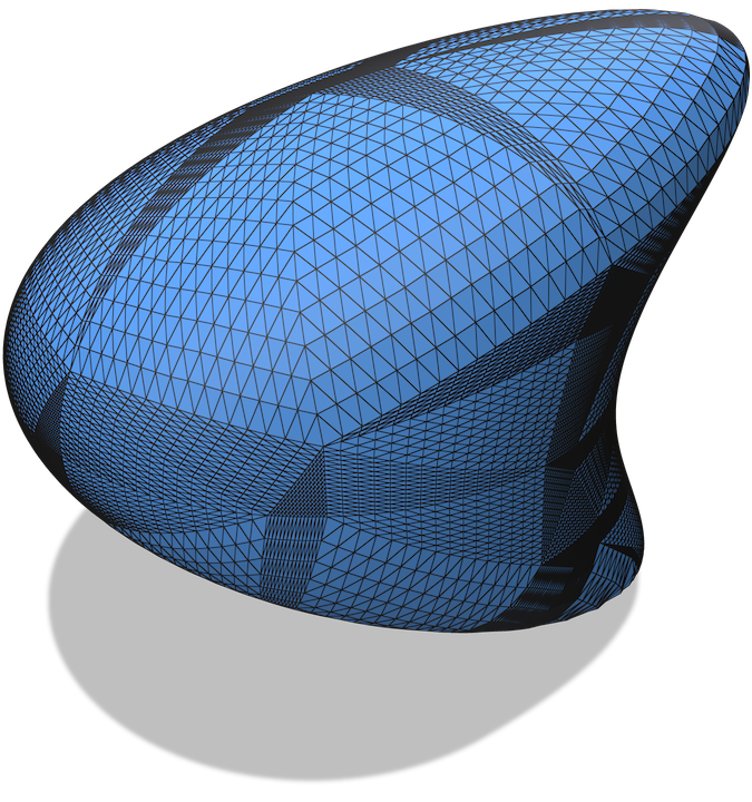
Figure 12. Triangulations of the Dziuk surface used for testing. Top-left: Good-quality base triangulation, $\mathcal{T}_{g}$. Top-right: Low-quality base triangulation, $\mathcal{T}_{b}$. Bottom row: The same triangulations after four rounds of refinement.

Triangle mesh resolution is measured as the mean edge-length in $\mathcal{T}_{g}$ or $\mathcal{T}_{b}$, whereas for CPM resolution is measured as the uniform $\Delta x$ used in the computational-tube $\Omega({\mathcal{S}})$. This core incompatibility makes it inappropriate to use resolution as the independent variable for comparative evaluations of error, computation time, or memory usage.

A more equitable comparison is to investigate computation time versus error and memory versus error. Computation times for CPM include the construction of $\Omega({\mathcal{S}})$ and $\Omega({\mathcal{C}})$ (which involves computing $\text{cp}_{{\mathcal{S}}}$ and $\text{cp}_{{\mathcal{C}}}$) and the time for constructing and solving the linear system. Computation times for the mesh-based method include the triangulation refinement and the construction and solution of the linear system. Evaluations are performed with ${\mathcal{C}}$ as a closed curve, an open curve, and a point since CPM IBC enforcement is slightly different for each type of ${\mathcal{C}}$.

Closed Curve IBC

The boundary curve ${\mathcal{C}}$ is constructed using the flip geodesics algorithm in geometry-central. The resulting ${\mathcal{C}}$ is represented as a polyline $\mathcal{P}$, which in general does not conform to edges or vertices of $\mathcal{T}$. For IBC enforcement, the nearest vertex in the triangulation $\mathcal{T}$ to each vertex in $\mathcal{P}$ is assigned the prescribed Dirichlet value.

This treatment of Dirichlet IBCs for the mesh-based method is first-order accurate in general. More accurate (and involved) Dirichlet IBC approaches could be used as discussed in Section 2.3. However, we set these options aside, as the goal of this comparison is simply to show that CPM with our first and second-order IBC approaches gives comparable results to basic mesh-based methods, that is, mesh-based methods where the representations of ${\mathcal{S}}$ and ${\mathcal{C}}$ are held fixed, e.g., no (extrinsic or intrinsic) remeshing is performed.

Figure 13 (top row) compares all types of CPM IBC approaches against the mesh-based method on $\mathcal{T}_{g}$ and $\mathcal{T}_{b}$ in columns (b) and (c). CPM with second-order IBCs achieves the lowest error for the same computation time and memory usage as other approaches. The mesh-based method with $\mathcal{T}_{g}$ outperforms the use of $\mathcal{T}_{b}$, as expected. CPM with first-order IBCs and nearest point approaches are similar and lie between the mesh-based method with $\mathcal{T}_{g}$ and $\mathcal{T}_{b}$. The method of Auer et al. (2012) has the largest error compared to all others. The expected order of convergence is seen for all CPM IBC approaches in the error versus $\Delta x$ plot of Figure 13 (top row, (d)).

Figure 13. A comparison of CPM vs. the mesh-based cotangent Laplacian for the Poisson equation with Dirichlet IBC. Top row: Closed curve ${\mathcal{C}}$. Middle row: Open curve ${\mathcal{C}}$. Bottom row: Point ${\mathcal{C}}$. Columns (b) and (c) show computation time vs. error and memory vs. error, respectively. Mesh results are shown separately for the $\mathcal{T}_{g}$ and $\mathcal{T}_{b}$ triangulations. Column (d) illustrates the convergence behaviour of error vs. $\Delta x$ for only the CPM schemes.

Open Curve IBC

The open curve ${\mathcal{C}}$ is also constructed using the flip geodesics algorithm in geometry-central. The Dirichlet IBC is enforced in the mesh-based solver in the same way as the closed curve above. Figure 13 (middle row) shows the same ranking of the methods as in the closed curve case, except CPM with first-order IBCs now outperforms both triangulations and the nearest point CPM approach. The expected order of convergence is seen for all CPM IBC approaches in Figure 13 (middle row, (d)).

Point IBC

The point ${\mathcal{C}}$ is intentionally chosen as one of the vertices in the base triangulation so that it is present in all refinements of $\mathcal{T}_{g}$ and $\mathcal{T}_{b}$. The Dirichlet IBC at ${\mathcal{C}}$ is imposed by replacing the vertex DOF in $\mathcal{T}$ with the prescribed Dirichlet value. Figure 13 (bottom row) shows the results for a point ${\mathcal{C}}$.

The mesh-based solver on $\mathcal{T}_{g}$ converges with second-order accuracy (since the IBC is a vertex), but only first-order accuracy on $\mathcal{T}_{b}$. Therefore, the mesh-based method with $\mathcal{T}_{g}$ outperforms CPM with second-order IBCs in the larger error regime. In the lower error regime, the latter methods are similar. All other methods show the same ranking as the open curve case. The expected order of convergence is seen for all CPM IBC approaches in Figure 13 (bottom row, (d)).

6.5. Linear System Solvers

Our partially matrix-free BiCGSTAB solver (see Section 5.4) is faster and more memory efficient than Eigen’s SparseLU and BiCGSTAB implementations (Guennebaud et al., 2010). An example of the improved efficiency is shown in Figure 14 for the heat problem in Section 6.2 with Dirichlet and zero-Neumann IBCs. Solving the heat equation involves multiple linear system solves (i.e., one for each time step). SparseLU requires the most computation time, even though it prefactors the matrix once and just performs forward/backward solves for each time step. SparseLU also uses the most memory, as expected.

Figure 14. Left pair: Computation time vs. $\Delta x$ plots for the heat equation (18) with Dirichlet and zero-Neumann IBCs with three solver options. Right pair: Memory vs. $\Delta x$ plots for the same problems and solvers. Our solver (orange) achieves the lowest computation time and memory costs at higher resolutions.

Table 2 gives the max and average computation time speedup, $T_{\rm{spdup}}$, and memory reduction, $M_{\rm{red}}$, for the results in Figure 14. The computation time speedup compared to Eigen’s SparseLU (similarly for BiCGSTAB) is computed as $T_{\rm{spdup}}=T(\rm{SparseLU})/T(\rm{Ours}),$ where $T(\rm{SparseLU})$ and $T(\rm{Ours})$ are the computation times of SparseLU and our solver, respectively. The memory reduction factor is calculated in an analogous manner with computation times replaced by memory consumption. The max and average $T_{\rm{spdup}}$ and $M_{\rm{red}}$ are computed over all $\Delta x$.

Solver	IBC	$T_{\rm{spdup}}$		$M_{\rm{red}}$
		Max	Avg.	Max	Avg.
Eigen’s SparseLU	Dirichlet	12.5	9.0	15.9	7.7
	Neumann	61.9	29.3	15.7	8.5
Eigen’s BiCGSTAB	Dirichlet	4.0	3.0	1.5	1.4
	Neumann	14.9	7.4	1.5	1.2

Table 2. Ratios of computation time $T_{\rm{spdup}}$ and memory usage $M_{\rm{red}}$ for Eigen’s SparseLU and BiCGSTAB as compared to our tailored BiCGSTAB solver, for the experiments of Figure 14.

The speedup of our solver is significant compared to both Eigen’s SparseLU and BiCGSTAB. The memory reduction of our method is significant compared to Eigen’s SparseLU, but less significant compared to Eigen’s BiCGSTAB. The speedup exhibits problem-dependence since $T_{\rm{spdup}}$ factors in Table 2 are larger for the zero-Neumann IBC compared to the Dirichlet IBC. However, as expected, $M_{\rm{red}}$ is not problem-dependent.

7. Applications

We now show the ability of our CPM approach to solve PDEs with IBCs that are common in applications from geometry processing: diffusion curves, geodesic distance, vector field design, and harmonic maps.

Quadratic polynomial interpolation, i.e., $p=2$, is used for all the examples in this section. Current CPM theory suggests that only first-order accuracy can be expected with quadratic polynomial interpolation, but CPM has been observed to give second-order convergence numerically (see (Macdonald and Ruuth, 2010), Section 4.1.1). This behaviour is confirmed with IBCs in Figure 15.

Figure 15. A comparison of CPM with quadratic vs. cubic interpolation stencils for the heat (top row) and Poisson (bottom row) problems of Figure 10 (b) and (d). Comparable results are achieved, but quadratic is often faster while cubic typically exhibits more regular convergence.

The main motivation for choosing quadratic interpolation is to obtain smaller computational tube-radii, $r_{\Omega({\mathcal{S}})}$, which allows higher curvature ${\mathcal{S}}$ and ${\mathcal{C}}$ to be handled with larger $\Delta x$. The resulting $\Omega({\mathcal{S}})$ and $\Omega({\mathcal{C}})$ contain fewer DOFs and therefore the computation is more efficient. Furthermore, Figure 15 shows that, for the same $\Delta x$, quadratic interpolation has lower computation times. Quadratic interpolation is 1.1-2.1 times faster than cubic interpolation in Figure 15. We used $p=3$ in the convergence studies of Section 6 because the error for second-order BCs with $p=2$ can sometimes be less regular (i.e., decreasing unevenly or non-monotonically) than with $p=3$ (Figure 15, bottom right).

CPM with first-order IBCs is used in all the examples in this section. The geodesic distance, vector field design, and harmonic map algorithms used here are themselves all inherently first-order accurate; hence using second-order IBCs would only improve accuracy near ${\mathcal{C}}$. Second-order IBCs could have been used for diffusion curves, but the first-order method was used for consistency.

7.1. Diffusion Curves

Diffusion curves offer a sparse representation of smoothly varying colours for an image (Orzan et al., 2008) or surface texture (Jeschke et al., 2009). Obtaining colours over all of ${\mathcal{S}}$ requires solving the surface Laplace equation with IBCs

(20) $$\Delta_{{\mathcal{S}}}u^{i}=0,\quad\rm{with}\quad\begin{cases}u^{i}=g^{i},\;\rm{or}\\ \nabla_{{\mathcal{S}}}u^{i}\cdot{\mathbf{b}}_{{\mathcal{C}}}=0.\end{cases}\rm{on}\;{\mathcal{C}}.$$

Laplace’s equation (20) is solved for each colour channel $u^{i}$ independently with CPM. The colour vector is composed of all the colour channels, e.g., for RGB colours ${\mathbf{u}}=[u^{1},u^{2},u^{3}]^{T}$. Dirichlet IBCs, $u^{i}=g^{i}$ on ${\mathcal{C}}$, are used to specify the colour values at sparse locations on ${\mathcal{S}}$. These colours spread over all of ${\mathcal{S}}$ when Laplace’s equation is solved. Zero-Neumann IBCs can also be used to treat ${\mathcal{C}}$ as a passive barrier that colours cannot cross. Two-sided IBCs along ${\mathcal{C}}$ are easily handled in our framework, and can even be of mixed Dirichlet-Neumann type (not to be confused with Robin BCs).

The surface of the Nefertiti bust is coloured by solving Laplace’s equation with CPM and IBCs specified by diffusion curves in Figure 3 (a). The surface triangulation is scaled (with fixed aspect ratio) to fit in $[-1,1]^{3}$ and $\Delta x=0.00315$ is used. IBC curves are polylines created using the flip geodesics algorithm in geometry-central (Sharp et al., 2019a). Most curves are two-sided Dirichlet IBCs (white curves, Figure 3 (a) left). However, the red and green band on the headdress is created using two-sided red-green Dirichlet IBCs vertically and two-sided Neumann-Dirichlet IBCs horizontally (black curves, Figure 3 (a) left).

The generality of CPM allows PDEs on mixed-codimensional surfaces to be solved. Figure 16 shows a diffusion curves example (with $\Delta x=0.05$) featuring a mixed 1D and 2D surface embedded in $\mathbb{R}^{3}$. This mixed-codimensional ${\mathcal{S}}$ is created using exact closest point functions for the torus, sphere, and line segment. The torus has minor radius $r=1$ and major radius $R=3$, while the sphere is of radius 1.25. The closest point to ${\mathcal{S}}$ is determined by computing the closest point to each of the torus, sphere, and line segments, then taking the closest of all four. The two curves ${\mathcal{C}}$ in this example are two-sided Dirichlet IBCs. ${\mathcal{C}}$ on the torus is a torus knot specified by the parametric equation

(21) $$x(s)=v(s)\cos(as),\quad y(s)=v(s)\sin(as),\quad z(s)=\sin(bs),$$

with $v(s)=R+\cos(bs),$ $a=3$, $b=7,$ and $s\in[0,2\pi]$. Closest points for the torus knot are computed using the optimization problem discussed in Appendix A. ${\mathcal{C}}$ on the sphere is an exact closest point function for a circle defined as the intersection of the sphere and a plane. Notice the colour from the torus to the sphere blends across the line segments as expected (see Figure 16 zoom).

Figure 16. Diffusion curves on a nonmanifold surface of mixed codimension. A pair of 1D segments connect the outer torus to the inner sphere.

Volumetric PDEs

Interestingly, CPM can also be applied to volumetric problems. A naive approach for volumetric problems embeds the hyper-planar surface ${\mathcal{S}}$ into $\mathbb{R}^{\rm{dim}({\mathcal{S}})+1}$. However, this is inefficient because unnecessary DOFs are included from the higher dimensional embedding space. A hyper-planar ${\mathcal{S}}$ can instead be embedded in $\mathbb{R}^{\rm{dim}({\mathcal{S}})}$, which corresponds to using CPM with $\rm{codim}({\mathcal{S}})=0$.

Consider a hyper-planar ${\mathcal{S}}$ with (irregular) boundary $\partial{\mathcal{S}}$. The computational domain $\Omega({\mathcal{S}})$ consists of all grid points ${\mathbf{x}}_{i}\in{\mathcal{S}}$ (having $\text{cp}_{{\mathcal{S}}}({\mathbf{x}}_{i})={\mathbf{x}}_{i}$) plus a layer of grid points outside ${\mathcal{S}}$ where $\text{cp}_{{\mathcal{S}}}({\mathbf{x}}_{i})\in\partial{\mathcal{S}}$ and $\|{\mathbf{x}}_{i}-\text{cp}_{{\mathcal{S}}}({\mathbf{x}}_{i})\|\leq r_{\Omega({\mathcal{S}})}.$

Figure 18 shows an example of applying CPM to the diffusion curves problem with ${\mathcal{S}}$ as the square $[-1,1]^{2}$ and $\Omega({\mathcal{S}})\subset\mathbb{R}^{2}.$

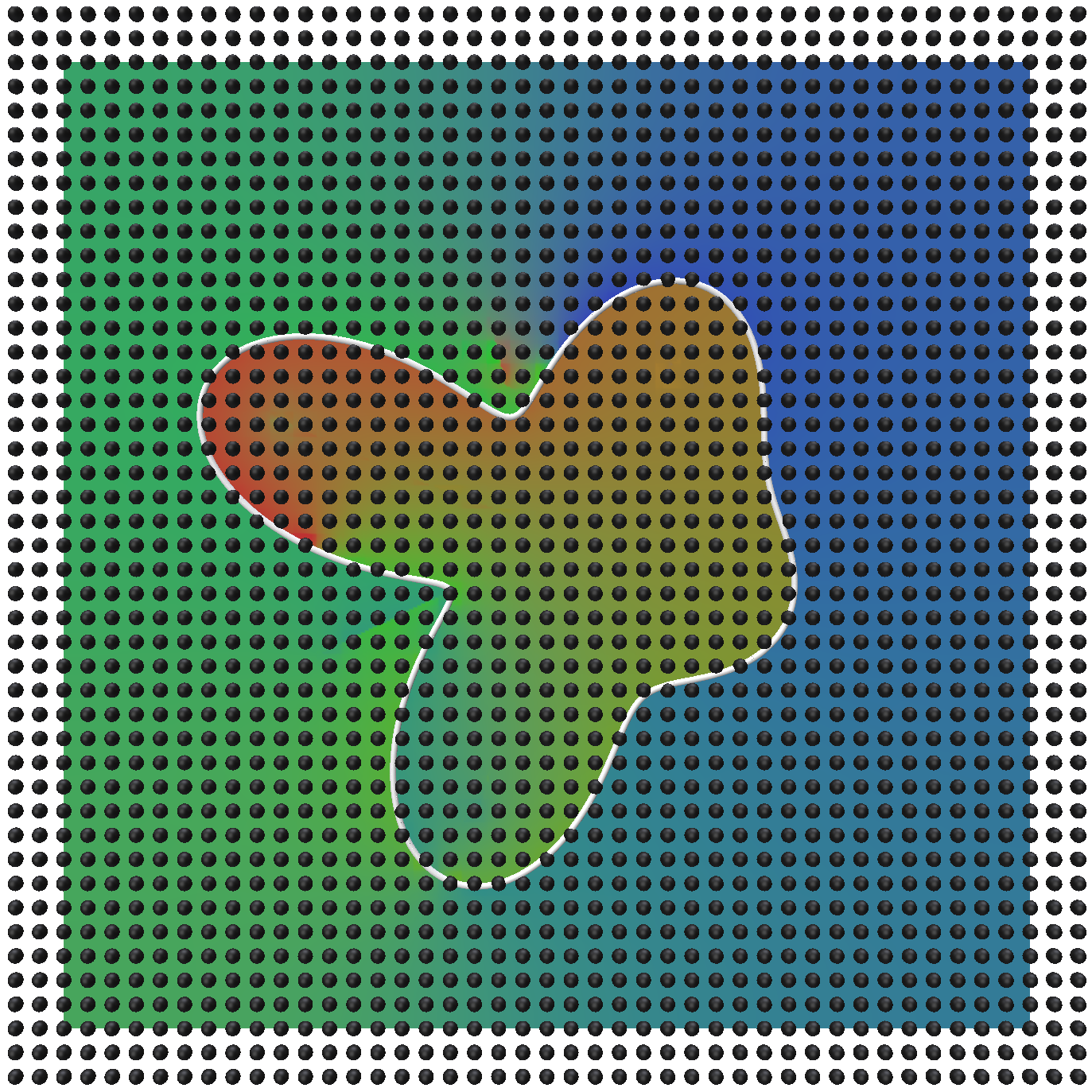
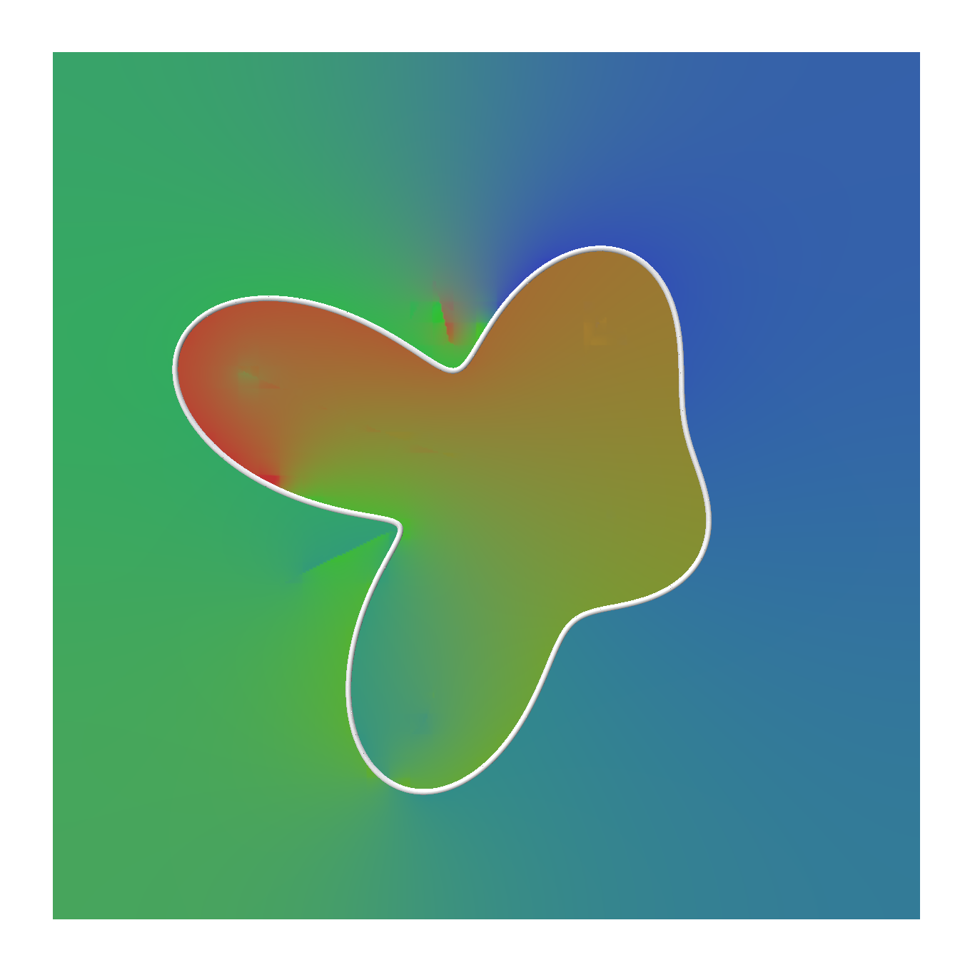
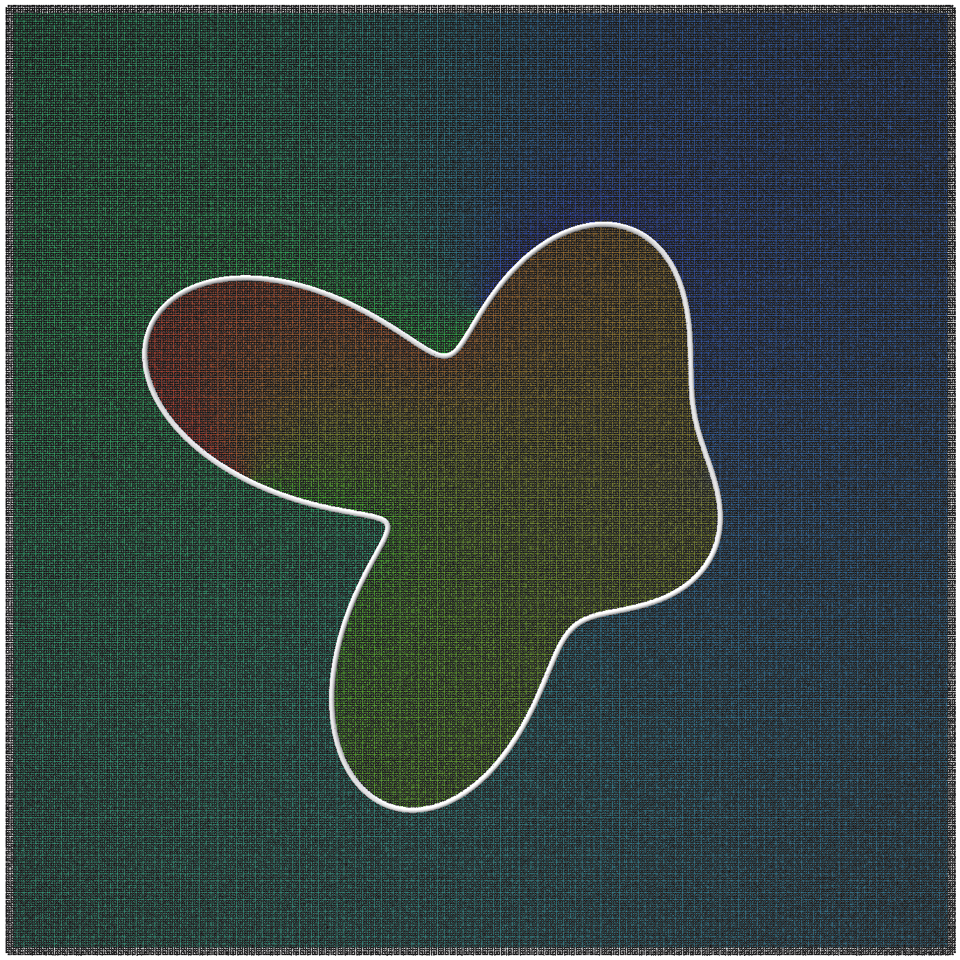
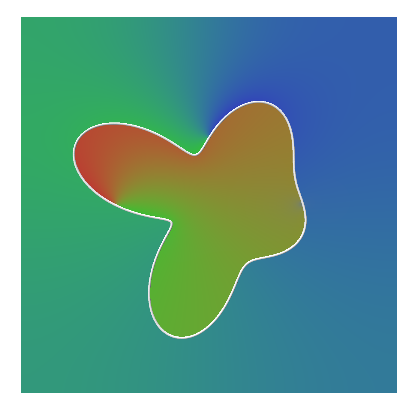
Figure 18. CPM applied to a codimension-zero diffusion curve problem, with the Dirichlet colour value varying along the white interior boundary curve. Top row: At an insufficient grid resolution of $\Delta x=0.05$ (left), high curvature regions exhibit errors near the curve’s medial axis (right). Bottom row: A high-resolution grid with $\Delta x=0.005$ (left) resolves the artifacts (right).

A parametric curve on the interior of ${\mathcal{S}}$ defines a diffusion curve ${\mathcal{C}}$ as a two-sided Dirichlet IBC, given by

(22) $$x(s)=v(s)\cos(s)+c,\quad y(s)=v(s)\sin(s)+c,$$

where

$$v(s)=\frac{\cos(s)\left(\frac{1}{2}(a+b)+\sin(as)+\sin(bs)\right)+\frac{1}{2}(a+b)}{a+b},$$

with $a=3$, $b=4$, $c=-\frac{1}{2},$ and $s\in[0,2\pi]$. Note that the colour varies along ${\mathcal{C}}$ from red to green inside ${\mathcal{C}}$ and blue to green outside ${\mathcal{C}}$. (Such colour variation along ${\mathcal{C}}$ can also easily be applied on non-hyper-planar ${\mathcal{S}}$.) First-order zero-Neumann exterior BCs are applied on $\partial{\mathcal{S}}$ naturally by CPM, which enforces no (conormal) colour gradient at $\partial{\mathcal{S}}$.

The grid spacing $\Delta x$ needs to be fine enough near ${\mathcal{C}}$ to give an accurate solution, in accordance with the requirements on the tube-radius (Section 3.1). Artifacts can occur if stencils undesirably cross the medial axis of ${\mathcal{C}}$ when $\Delta x$ is too large (cf. Figure 18 top and bottom rows). A promising direction of future work is therefore to explore the use of adaptive grids based on the geometry of ${\mathcal{C}}$. Adaptivity would reduce the total number of DOFs in the linear system and thus improve efficiency. Adaptive grids based on the geometry of ${\mathcal{S}}$ would also improve efficiency for problems with $\rm{codim}({\mathcal{S}})>0$.

Applying CPM with $\rm{codim}({\mathcal{S}})=0$ represents an alternative to (or generalization of) various existing embedded boundary methods for irregular domains, e.g., (Gibou et al., 2002; Ng et al., 2009; Schwartz et al., 2006). Advantages and disadvantages of this approach should be explored further in future work. One advantage shown by Macdonald et al. (2013) is the ability to couple volumetric and surface PDEs in a unified framework.

7.2. Geodesic Distance

The heat method for geodesic distance computation (Crane et al., 2013) has been implemented on many surface representations, including polygonal surfaces, subdivision surfaces (De Goes et al., 2016b), spline surfaces (Nguyen et al., 2016), tetrahedral meshes (Belyaev and Fayolle, 2015), and point clouds (Crane et al., 2013), with each requiring nonnegligible tailoring and implementation effort. By introducing our Dirichlet IBC treatment for CPM, we have enabled a single implementation covering all these cases, since closest points can be computed to these and many other surface representations.

The heat method approximates the geodesic distance $\phi$ using the following three steps:

1. Solve $\frac{\partial u}{\partial t}=\Delta_{{\mathcal{S}}}u$ to give $u_{t}$ at time $t,$

2. Evaluate the vector field $\mathbf{X}=-\nabla_{{\mathcal{S}}}u_{t}/\|\nabla_{{\mathcal{S}}}u_{t}\|,$

3. Solve $\Delta_{{\mathcal{S}}}\phi=\nabla_{{\mathcal{S}}}\cdot\mathbf{X}$ for $\phi$.

Step (1) uses a Dirac-delta heat source for a point ${\mathcal{C}}$ or a generalized Dirac distribution over a curve ${\mathcal{C}}$ as the initial condition. The approximation in time of step (1) uses implicit Euler, for one time-step, which is equivalent (up to a multiplicative constant) to solving

(23) $$(\mathbf{I}-t\Delta_{{\mathcal{S}}})v_{t} =0\;\text{ on }\;{\mathcal{S}}\backslash{\mathcal{C}},$$

$$v_{t} =1\;\text{ on }\;{\mathcal{C}}.$$

The discrete system for (23) can be written as $\mathbf{A}\mathbf{v}=\mathbf{f}$, where $\mathbf{A}\in\mathbb{R}^{(N_{{\mathcal{S}}}+N_{{\mathcal{C}}})\times(N_{{\mathcal{S}}}+N_{{\mathcal{C}}})}$ and $\mathbf{v},\mathbf{f}\in\mathbb{R}^{N_{{\mathcal{S}}}+N_{{\mathcal{C}}}}$.

Imposing first-order IBCs involves the Heaviside step function for $\mathbf{f}$. That is, $\mathbf{f}_{i}=0$ if $i$ is in the PDE DOF set ($i\in J_{{\mathcal{S}}}$) and $\mathbf{f}_{i}=1$ if $i$ is in the BC DOF set ($i\in J_{{\mathcal{C}}}$). When imposing this IBC in (23), CPM can experience Gibb’s phenomenon due to the polynomial interpolation used for the CP extension. Therefore, we approximate the Heaviside step function with a smooth approximation as

$$\mathbf{f}_{i}=\frac{1}{2}{\rm tanh}\left(-k\|\text{cp}_{\mathcal{S}-\mathcal{C}}(\mathbf{x}_{i})\|\right)+\frac{1}{2},\quad{\rm with}\quad k=\frac{\rm{atanh}(1-\epsilon)}{e}.$$

The parameters $e$ and $\epsilon$ correspond to the “extent” $[-e,e]$ and the maximum error of the approximation outside of the extent, respectively. That is, when $\|\text{cp}_{\mathcal{S}-\mathcal{C}}(\mathbf{x}_{i})\|=e$, the error in approximating the Heaviside function is $\epsilon$ and the error becomes smaller further outside of $[-e,e]$. We choose $e=r_{\Omega({\mathcal{S}})}$ and $\epsilon=\Delta x$ for the results here.

Step (3) of the heat method also involves a Dirichlet IBC, $\phi=0$ on ${\mathcal{C}}$, since the geodesic distance is zero for points on ${\mathcal{C}}$. No special treatment is required for this IBC. To improve accuracy steps (2) and (3) are applied iteratively as discussed by Belyaev and Fayolle (2015). Two extra iterations of steps (2) and (3) are applied in all our examples of the CPM-based heat method.

We use Eigen’s SparseLU to solve (only) the linear systems arising from step (1) of the heat method. Using BiCGSTAB (either Eigen’s or our custom solver) results in an incorrect solution despite the iterative solver successfully converging, even under a relative residual tolerance of $10^{-15}$. We observed that the small time-step of the heat method, $\Delta t=\Delta x^{2},$ causes difficulties for BiCGSTAB. The reason is that values far from the heat sources are often extremely close to zero. Tiny errors in these values are tolerated by BiCGSTAB, but lead to disastrously inaccurate gradients in step (2), and thus incorrect distances in step (3). (An alternative would be to compute smoothed distances (see Section 3.3 of (Crane et al., 2013)), by using larger time-steps of $\Delta t=m\Delta x^{2}$ with $m\geq 100$; in this case BiCGSTAB exhibits no issues.) Our partially matrix-free BiCGSTAB solver is nevertheless successfully used for step (3) of the heat method.

Figure 19 shows the geodesic distance to a single source point on the Dziuk surface, where our CPM-based approach (with $\Delta x=0.0125$) is compared to exact polyhedral geodesics (Mitchell et al., 1987) and the mesh-based heat method. Implementations of the latter two methods are drawn from geometry-central (Sharp et al., 2019a). All three approaches yield similar results.

Exact Polyhedral

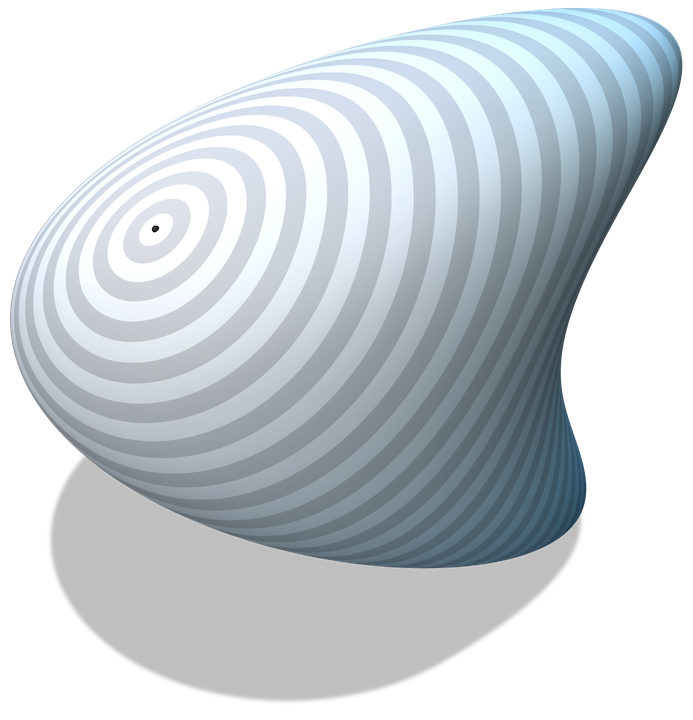
CPM Heat Method (Ours)

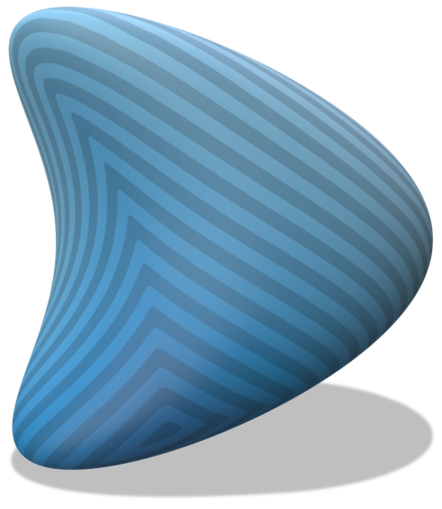
Mesh Heat Method

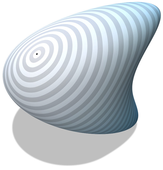
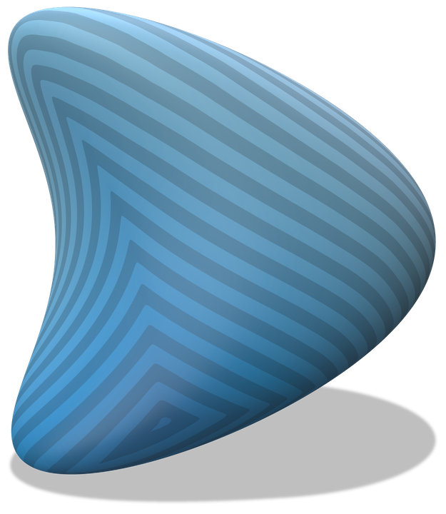
Figure 19. A comparison of CPM vs. mesh-based methods for geodesic distances to a point on the Dziuk surface. Consistent results are observed.

For the example in Figure 19, closest points are computed from the same triangulation used in the exact polyhedral and mesh-based heat method. However, closest points can also be directly computed from the level-set Dziuk surface (as in Section 6.3). To our knowledge, the heat method has not been applied on level-set surfaces before.

We showcase the ability of our CPM to compute geodesic distance on general surface representations. Figure 21 visualizes the geodesic distance to an open curve on the “DecoTetrahedron” (Palais et al., 2023) level-set surface,

$${\mathcal{S}}=\bigg{\{}{\mathbf{x}}\in\mathbb{R}^{3}\;\bigg{|}\; \sum_{i=1}^{3}\left((x_{i}-2)^{2}(x_{i}+2)^{2}-10x_{i}^{2}\right)$$

$$+3\left(x_{1}^{2}x_{2}^{2}+x_{1}^{2}x_{3}^{2}+x_{2}^{2}x_{3}^{2}\right)+6x_{1}x_{2}x_{3}=-22\bigg{\}}.$$

${\mathcal{S}}$ and ${\mathcal{C}}$ can also have mixed representations. For example, Figure 3 (b) shows the geodesic distance (using $\Delta x=0.00625$) to the trefoil knot (a.k.a. torus knot with $a=2$ and $b=3$, see (21)) on a torus with minor and major radii 1 and 2, respectively. The trefoil knot uses a parametric representation while the torus uses an exact closest point representation.

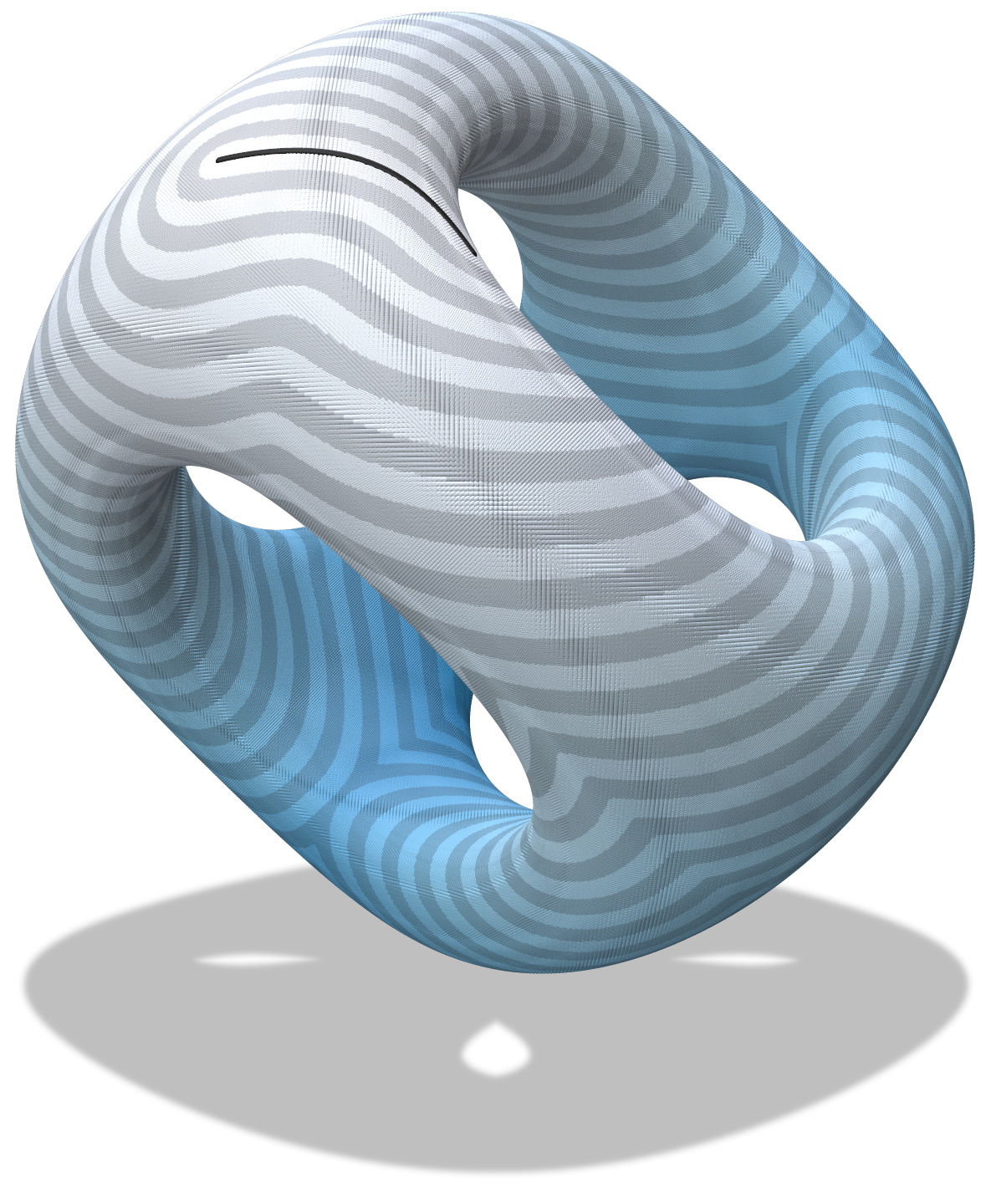
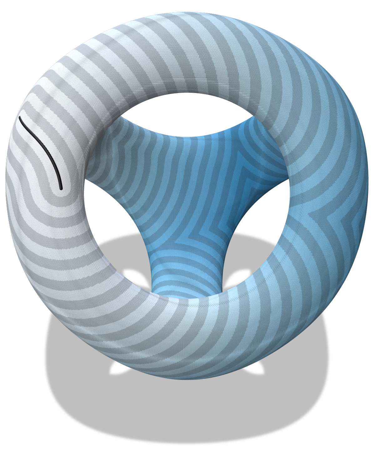
Figure 21. Geodesic distance to a curve (black) visualized on the “DecoTetrahedron” level-set surface computed using CPM with $\Delta x=0.025$. The closest points themselves are directly rendered.

7.3. Vector Field Design

Designing tangent vector fields on surfaces is useful in many applications including texture synthesis, non-photorealistic rendering, quad mesh generation, and fluid animation (De Goes et al., 2016a; Zhang et al., 2006). One approach for vector field design involves the user specifying desired directions at a sparse set of surface locations, which are then used to construct the field over the entire surface. Adapting ideas from Turk (2001) and Wei and Levoy (2001), we interpret the user-specified directions as Dirichlet IBCs and use diffusion to obtain the vector field over the whole surface.

We iterate between heat flow of the vector field and projections onto the tangent space to obtain the tangent vector field over all of ${\mathcal{S}}$. Specifically, each iteration involves the following steps:

1. Perform heat flow independently for each component of ${\mathbf{u}}=[u^{1},u^{2},u^{3}]^{T}$ according to

   $$\frac{\partial u^{i}}{\partial t}=\Delta_{{\mathcal{S}}}u^{i},\quad\rm{with}\quad\begin{cases}u^{i}=g^{i},\;\rm{or}\\ \nabla_{{\mathcal{S}}}u^{i}\cdot{\mathbf{b}}_{{\mathcal{C}}}=0,\end{cases}\rm{on}\;{\mathcal{C}},$$

   starting from the vector field after the previous iteration.

2. Project ${\mathbf{u}}({\mathbf{x}}_{i})$ onto the tangent space of ${\mathcal{S}}$ using ${\mathbf{n}}_{{\mathcal{S}}}$ at $\text{cp}_{{\mathcal{S}}}({\mathbf{x}}_{i})$

   $${\mathbf{u}}({\mathbf{x}}_{i})=(\mathbf{I}-{\mathbf{n}}_{{\mathcal{S}}}{\mathbf{n}}_{{\mathcal{S}}}^{T}){\mathbf{u}}({\mathbf{x}}_{i}).$$

One time-step of heat flow is performed on each iteration using implicit Euler with $\Delta t=0.1\Delta x.$ A total of 10 iterations are used for all examples. The vector field for the first iteration consists of zero vectors unless the direction is specified by an IBC.

Dirichlet IBCs $\mathbf{g}=[g^{1},g^{2},g^{3}]^{T}$ can be specified at points or curves. For point Dirichlet IBCs the direction of $\mathbf{g}$ is any direction in the tangent space of ${\mathcal{S}}$. Dirichlet IBCs on curves could also specify any direction in the tangent space of ${\mathcal{S}}$, but designing vector fields is more intuitive when $\mathbf{g}$ is the tangent direction ${\mathbf{t}}_{{\mathcal{C}}}$ along ${\mathcal{C}}$. Zero-Neumann IBCs are also used within our framework to block the vector field from diffusing across ${\mathcal{C}}$.

Figure 3 (c) shows an example of a vector field designed on the Möbius strip. The Möbius strip is actually a triangulated surface in this example, although its parametric form could be used instead (see (Macdonald et al., 2011)). The triangulation is scaled (with fixed aspect ratio) to fit in $[-1,1]^{3}$ and $\Delta x=0.0064$ is used. Zero-Neumann exterior BCs are imposed automatically by CPM with first-order accuracy on the geometric boundary. This example shows the ability of our approach to handle open and nonorientable surfaces. There are four points and two curves specifying the IBCs in Figure 3 (c). A circular closed curve demonstrates that vortices can be created. The other curve on the Möbius strip enforces a zero-Neumann IBC that blocks direction changes in the vector field (see Figure 3 (c) zoom).

Figure 22. Vector field design on a parametric surface of revolution, with Dirichlet IBC curve and points shown in white.

Figure 22 shows another example on a parametric surface of revolution (with $\Delta x=0.025$), which is constructed by revolving the planar parametric curve (22) with $c=\frac{1}{2}$ around the $z$-axis. All IBCs in this example are Dirichlet IBCs. Sinks and sources in the vector field are created with four Dirichlet point IBCs. The curve IBC is a two-sided Dirichlet IBC that flips the direction of the vector field across ${\mathcal{C}}$ (see Figure 22 zoom).

7.4. Harmonic Maps

A map between two surfaces, ${\mathcal{S}}_{1}$ and ${\mathcal{S}}_{2}$, matches locations on ${\mathcal{S}}_{1}$ with locations on ${\mathcal{S}}_{2}$. The map can be used to analyze differences between ${\mathcal{S}}_{1}$ and ${\mathcal{S}}_{2}$ or to transfer data from one surface to the other. Harmonic maps are a specific type of map that appears in numerous domains, e.g., mathematical physics (Bartels, 2005) and medical imaging (Shi et al., 2007, 2009). In computer graphics, harmonic maps can be used for many applications such as texture transfer, quad mesh transfer, and interpolating intermediate poses from key-frames of a character (Ezuz et al., 2019).

King and Ruuth (2017) considered applying CPM to compute harmonic maps ${\mathbf{u}}({\mathbf{y}}):{\mathcal{S}}_{1}\rightarrow{\mathcal{S}}_{2}$. Adapting their approach, we compute the harmonic map using the gradient descent flow

(24) $$\frac{\partial{\mathbf{u}}}{\partial t} =\Pi_{T_{{\mathbf{u}}}{\mathcal{S}}_{2}}(\Delta_{{\mathcal{S}}_{1}}{\mathbf{u}}),$$

$${\mathbf{u}}({\mathbf{y}},0) =\mathbf{f}({\mathbf{y}}),$$

$${\mathbf{u}}({\mathbf{y}},t) =\mathbf{g}({\mathbf{y}}),\;\rm{for}\;{\mathbf{y}}\in{\mathcal{C}}_{1},$$

where $\Pi_{T_{{\mathbf{u}}}{\mathcal{S}}_{2}}$ is the projection operator at the point ${\mathbf{u}}$ onto the tangent space of ${\mathcal{S}}_{2}$. The vector $\Delta_{{\mathcal{S}}_{1}}{\mathbf{u}}$ is defined componentwise, i.e., $\Delta_{{\mathcal{S}}_{1}}{\mathbf{u}}=[\Delta_{{\mathcal{S}}_{1}}u^{1},\Delta_{{\mathcal{S}}_{1}}u^{2},\Delta_{{\mathcal{S}}_{1}}u^{3}]^{T}.$ The $\mathbf{f}({\mathbf{y}})$ and $\mathbf{g}({\mathbf{y}})$ are the initial map (from ${\mathcal{S}}_{1}$ to ${\mathcal{S}}_{2}$) and the landmark map (from ${\mathcal{C}}_{1}\subset{\mathcal{S}}_{1}$ to ${\mathcal{C}}_{2}\subset{\mathcal{S}}_{2}$), respectively. The subsets ${\mathcal{C}}_{1}$ and ${\mathcal{C}}_{2}$ can be landmark points or curves on ${\mathcal{S}}_{1}$ and ${\mathcal{S}}_{2}$ that are enforced to match using our new Dirichlet IBC treatment; such IBCs were not considered by King and Ruuth (2017).

An operator splitting approach was used by King and Ruuth (2017), which allows (24) to be solved with a PDE on ${\mathcal{S}}_{1}$ alone. Specifically, one time-step consists of the following:

1. Solve (24) without the $\Pi_{T_{{\mathbf{u}}}{\mathcal{S}}_{2}}$ term using CPM on $\Omega({\mathcal{S}}_{1})$ with $\Omega({\mathcal{C}}_{1})$ to enforce the IBC.

2. Project the solution from (1) onto ${\mathcal{S}}_{2}$.

Denote the solution from step (1) at ${\mathbf{x}}_{i}\in\Omega({\mathcal{S}}_{1})$ and time-step $k$ by ${\mathbf{v}}^{k}_{i}$. The projection in step (2) simply moves ${\mathbf{v}}^{k}_{i}$ to its closest point on ${\mathcal{S}}_{2}$ by setting ${\mathbf{u}}^{k}_{i}=\text{cp}_{{\mathcal{S}}_{2}}({\mathbf{v}}^{k}_{i})$. One time-step of explicit Euler is used for step (1) with $\Delta t=0.1\Delta x^{2}$ starting from ${\mathbf{u}}^{k-1}$.

To perform the above gradient descent flow a valid initial map ${\mathbf{u}}^{0}$ is needed to start from. Generating such initial maps in the general case has not yet been addressed for CPM (King and Ruuth, 2017). Approaches based on geodesic distance to landmark curves/points ${\mathcal{C}}_{1},$ ${\mathcal{C}}_{2}$ could potentially be adapted (Ezuz et al., 2019; Shi et al., 2007). However, for our illustrative example of incorporating IBCs while computing harmonic maps, we opt for a simple (but restrictive) initial map construction. The surface ${\mathcal{S}}_{1}$ is given by a triangulation and deformed to create ${\mathcal{S}}_{2}$ while maintaining the same vertex connectivity. Therefore, the barycentric coordinates of each triangle can be used to initially map any point on ${\mathcal{S}}_{1}$ to a point on ${\mathcal{S}}_{2}$.

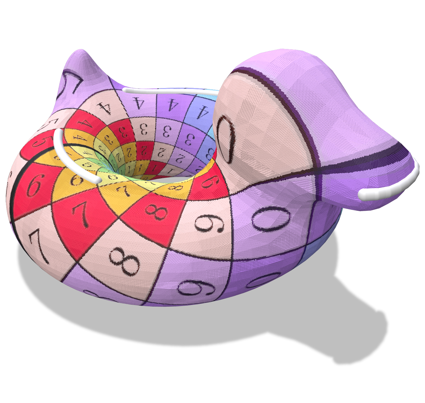
(a) ${\mathcal{S}}_{1}$ with Texture

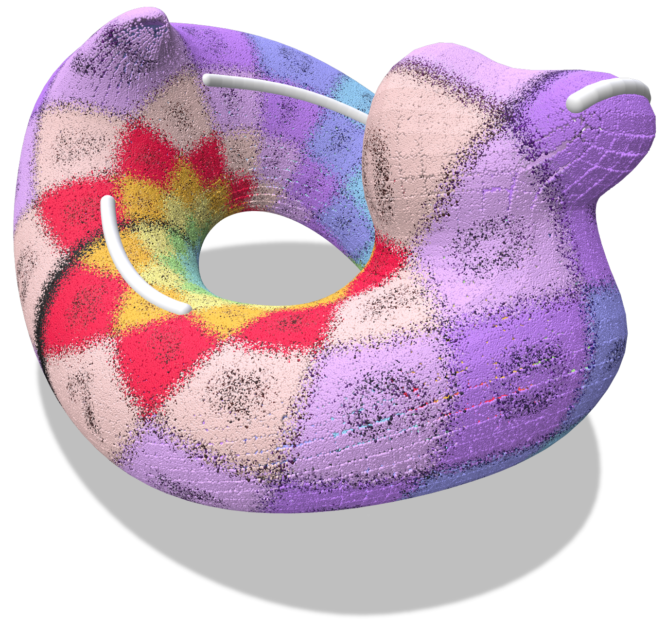
(b) Initial Map onto ${\mathcal{S}}_{2}$

(c) Harmonic Map onto ${\mathcal{S}}_{2}$ w/o IBCs

(d) Harmonic Map onto ${\mathcal{S}}_{2}$ w/ IBCs

Figure 24. Maps from ${\mathcal{S}}_{1}$ to ${\mathcal{S}}_{2}$ with a texture for visualizing the mapping. Landmark curves (Dirichlet IBCs) ${\mathcal{C}}_{1}$ and ${\mathcal{C}}_{2}$ are shown in white. (a) ${\mathcal{S}}_{1}$ with texture. (b) ${\mathcal{S}}_{2}$ with texture from a noisy initial map. (c) ${\mathcal{S}}_{2}$ with a CPM harmonic mapped texture without IBCs. (d) ${\mathcal{S}}_{2}$ with a harmonic mapped texture using our CPM approach satisfying the IBCs. The surface is displayed using the closest points.

Figure 24 shows an example of computing harmonic maps from the Bob surface ${\mathcal{S}}_{1}$ to its deformed version ${\mathcal{S}}_{2}$. The triangulation of ${\mathcal{S}}_{1}$ is scaled (with fixed aspect ratio) to fit in $[-1,1]^{3}$ and $\Delta x=0.00663$ is used for $\Omega({\mathcal{S}}_{1})$. A texture is added to the surface of ${\mathcal{S}}_{1}$ and transferred to ${\mathcal{S}}_{2}$ through the mapping ${\mathbf{u}}$. To emphasize the effect of computing the harmonic map, noise is added to the initial map (see Figure 24 (b)) before performing the gradient descent flow. The gradient descent flow is evolved to steady state using 200 time steps. Figure 24 shows the harmonic map with and without Dirichlet IBCs. The harmonic map with Dirichlet IBCs distorts near ${\mathcal{C}}_{2}$ to satisfy both the PDE and IBCs (cf. Figure 24 (c) and (d) zoom). This distortion is expected unless the IBC $\mathbf{g}$ is harmonic itself.

8. Limitations and Future Work

As we have discussed and demonstrated, CPM is a powerful tool for solving surface PDEs since it provides a unified framework for general surface characteristics, general surface representations, and general PDEs. Our work extends CPM to solve surface PDEs with interior boundary conditions (Dirichlet and zero-Neumann) while obtaining up to second-order accuracy. The ability to enforce IBCs enables CPM to be applied to many PDE-based geometry processing tasks and applications, which were not previously possible. Additionally, we have developed a runtime and memory-efficient implementation allowing for the treatment of higher-detail surfaces without specialized hardware. To encourage wider adoption of CPM, we will make the code for our framework publicly available, upon acceptance of this paper. Below, we outline some of CPM’s existing limitations and describe a few exciting directions for future work.

BC Types, Higher-Order Accuracy, and Other PDEs

CPM work to date has only addressed Dirichlet and zero-Neumann (exterior) BCs. Macdonald et al. (2013) solved a surface-to-bulk coupled PDE with Robin BCs on the boundary of the bulk (but ${\mathcal{S}}$ was closed, i.e., $\partial{\mathcal{S}}=\emptyset$). Extending CPM to impose nonhomogeneous-Neumann, Robin, and other types of BCs is an important area of future work. Fortunately, the interior BC framework developed here directly generalizes existing CPM approaches for exterior BCs; therefore, our work likely makes any future extensions of CPM for other exterior BC types immediately applicable as interior BCs as well.

Third-order and higher (exterior and interior) BCs are also important for higher-order PDE discretizations. CPM with higher-order exterior BCs has not yet been explored, although Macdonald et al. (2011) point out that a replacement for $\overline{\text{cp}}_{{\mathcal{S}}}$ is required to incorporate the curvature of ${\mathcal{S}}$ near $\partial{\mathcal{S}}$. For higher-order interior BCs an improved ${\mathcal{S}}_{\perp}$ crossing test (12), involving curvatures of ${\mathcal{S}}$ near ${\mathcal{C}},$ is likely also needed.

We have focused on problems involving the ubiquitous Laplace-Beltrami operator, but CPM has been applied to numerous other PDEs (see Section 2). In principle, our approach to IBC enforcement should also readily extend to those settings. Extending CPM to approximate previously unexplored operators, such as the relative Dirac operator (Liu et al., 2017) or the connection Laplacian (Sharp et al., 2019c), would allow other geometry processing applications to benefit from CPM.

Efficiency

The discrete setup using a uniform grid near ${\mathcal{S}}$ was chosen for its simplicity and use of well-studied Cartesian numerical methods (i.e., Lagrange interpolation and finite differences). However, the radius of CPM’s computational tube is dictated by the curvature and/or bottlenecks of ${\mathcal{S}}$ and ${\mathcal{C}}$ (see Section 3.1). Higher curvatures or narrow bottlenecks force the uniform grid spacing to be small, leading to inefficiency due to a large number of DOFs.

One way to improve the runtime and memory efficiency of CPM on uniform grids is to use parallelization on specialized hardware, e.g., GPU (Auer et al., 2012) or distributed memory (May et al., 2022). However, the number of DOFs with a uniform grid can be higher than necessary, since the grid is allowed to be coarser in low curvature regions and away from tight bottlenecks of ${\mathcal{S}}$ and ${\mathcal{C}}$. Near bottlenecks with low curvature, duplicate DOFs on either side of the medial axis could be introduced to avoid refining while ensuring data is extended from the correct part of ${\mathcal{S}}$ (similar to how the current work distinguishes different sides of an IBC). Conversely, near high curvature regions, spatial adaptivity (e.g., octrees) could be used to provide locally higher resolution. Combining duplicate DOFs and adaptivity is, therefore, a promising direction to make CPM more efficient (both in runtime and memory) for complex surfaces, without recourse to specialized hardware.

Exploring other approximations of the CP extension and differential operators in the Cartesian embedding space could also improve efficiency. For example, combining Monte Carlo methods (Sawhney and Crane, 2020; Sawhney et al., 2022; Rioux-Lavoie et al., 2022; Sugimoto et al., 2023) with CPM is one interesting avenue. Monte Carlo methods can avoid computing the global solution, so they may be more efficient when the solution is only desired on a local portion of ${\mathcal{S}}$.

Smoothness of ${\mathcal{S}}$ and ${\mathcal{C}}$

Most CPM work and theory is based on $C^{2}$-smooth surfaces. However, WENO interpolation has been used to improve the grid-based CPM (i.e., the form used in this paper) for nonsmooth surfaces (e.g., surfaces with sharp features) (Macdonald and Ruuth, 2008; Auer et al., 2012). Cheung et al. (2015) used duplicated DOFs (similar to the current work) near the sharp feature with an RBF discretization of CPM. However, RBF discretizations can suffer from ill-conditioned linear systems. Therefore, it would be interesting to instead explore altering stencils (similar to our IBC approach) for the grid-based CPM near sharp features to use data from the “best side” of the sharp feature. In this context, the BC curve ${\mathcal{C}}$ would instead be the sharp feature and the PDE is still imposed on ${\mathcal{C}}$ instead of a BC.

The theoretical restriction of $C^{2}$ smoothness also applies to the curve ${\mathcal{C}}$. Therefore, our IBC approach is theoretically restricted to curves without kinks or intersections. In practice, we are still able to obtain the expected result when ${\mathcal{C}}$ has sharp features or intersections, e.g., Figure 3 (a) involves many intersecting curves (in the band of the headdress) that also create sharp corners. Theoretical understanding of what CPM does near sharp features and intersections is interesting future work.

CPM offers an exciting, unified framework for surface PDEs on “black box” closest point surfaces, which we have extended with accurate interior BCs. The discussion above has outlined a partial roadmap of CPM’s significant untapped potential; we hope that others in the computer graphics community join us in exploring it.

APPENDIX

Appendix A Closest Point Computation

Some surfaces allow closest points to be computed analytically, e.g., lines, circles, planes, spheres, cylinders, and tori. We use the analytical expressions for exact closest points in all examples for which they exist. For parameterized surfaces, closest points can be computed using standard numerical optimization techniques, e.g., Ruuth and Merriman (2008) used Newton’s method for various surfaces, such as a helix. For examples in this paper, we solve

$$\operatorname*{argmin}_{\mathbf{t}}\frac{1}{2}\|\mathbf{p}(\mathbf{t})-{\mathbf{x}}_{i}\|^{2},$$

for the surface parameters $\mathbf{t}$ (e.g., $\mathbf{t}=t$ for a 1D surface and $\mathbf{t}=[u,v]^{T}$ for a 2D surface), where $\mathbf{p}(\mathbf{t})\in{\mathcal{S}}$ and ${\mathbf{x}}_{i}\in\Omega({\mathcal{S}})$. LBFGS++ (Qiu, 2023) is used to solve the optimization problem. An initial guess for $\text{cp}_{{\mathcal{S}}}({\mathbf{x}}_{i})$ is taken as the nearest neighbour in a point cloud $\mathcal{P}_{{\mathcal{S}}}$ of the parametric surface. The point cloud $\mathcal{P}_{{\mathcal{S}}}$ is constructed using $N$ equispaced points of the parameter $\mathbf{t}$.

Computing closest points to triangulated surfaces is also well-studied (Strain, 1999; Mauch, 2003; Auer et al., 2012). Notably, the work of Auer et al. (2012) implements the closest point evaluation on a GPU. There also exist open source libraries that support computing closest points to triangle meshes, e.g., libigl (Jacobson et al., 2018). Here we use the library fcpw (Sawhney, 2022) to compute closest points to triangulated surfaces and polyline curves.

The simplest way to compute closest points to a point cloud is to take the nearest neighbour as the closest point. As discussed by Macdonald et al. (2013) this choice can be inaccurate if the point cloud is not dense enough. Wang et al. (2020) (Figure 17) showed the inaccuracy of using nearest neighbours as closest points with CPM on a diffusion problem. Several more accurate approaches for closest points to point clouds have been developed (Martin and Tsai, 2020; Petras et al., 2022; Liu et al., 2006; Yingjie and Liling, 2011).

Closest points can also be computed from exact signed-distance functions $d({\mathbf{x}})$ as

(25) $$\text{cp}_{{\mathcal{S}}}({\mathbf{x}})={\mathbf{x}}-d({\mathbf{x}})\nabla d({\mathbf{x}}).$$

Equation (25), however, is not valid for more general level-set functions $\phi$. High-order accuracy of closest points from level-set functions (sampled on a grid) can be obtained using the method of Saye (2014). For the examples in this paper, we use the ideas of Saye (2014) but with analytical expressions for $\phi$. Specifically, an initial guess $\text{cp}^{\star}$ of the closest point is obtained using a Newton-style procedure, starting with $\text{cp}_{0}={\mathbf{x}}_{i},$ and iterating

$$\text{cp}_{k+1}=\text{cp}_{k}-\frac{\phi(\text{cp}_{k})\nabla\phi(\text{cp}_{k})}{\|\nabla\phi(\text{cp}_{k})\|^{2}},$$

with stopping criterion $\|\text{cp}_{k+1}-\text{cp}_{k}\|<10^{-10}.$ Then Newton’s method

$${\mathbf{y}}_{k+1}={\mathbf{y}}_{k}-(D^{2}f({\mathbf{y}}_{k}))^{-1}\nabla f({\mathbf{y}}_{k}),$$

is used to optimize

$$f(\text{cp},\lambda)=\frac{1}{2}\|\text{cp}-{\mathbf{x}}_{i}\|^{2}+\lambda\phi(\text{cp}),$$

where ${\mathbf{y}}=[\text{cp},\lambda]^{T}$ and $\|{\mathbf{y}}_{k+1}-{\mathbf{y}}_{k}\|<10^{-10}$ is used as the stopping criterion. The initial Lagrange multiplier is $\lambda_{0}=({\mathbf{x}}_{i}-\text{cp}^{\star})\cdot\nabla\phi(\text{cp}^{\star})/\|\nabla\phi(\text{cp}^{\star})\|^{2}$. Analytical expressions for $\nabla f({\mathbf{y}})$ and $D^{2}f({\mathbf{y}})$ are computed using analytical expressions of $\nabla\phi$ and $D^{2}\phi$.

Closest points for surfaces composed of multiple surfaces can be computed by obtaining the closest point to each independent surface first. Then the closest point to the combined surface is taken as the closest of the independent surface closest points (e.g., the torus and sphere joined by line segments in Figure 16).

Closest points can be computed for many other surface representations. For example, closest points to neural implicit surfaces can be computed using the work of Sharp and Jacobson (2022). Further references for closest point computation are given in Section 5.1 of (Sawhney and Crane, 2020).

References

- (1)
- Aamari et al. (2019) Eddie Aamari, Jisu Kim, Frédéric Chazal, Bertrand Michel, Alessandro Rinaldo, and Larry Wasserman. 2019. Estimating the reach of a manifold. Electronic Journal of Statistics 13, 1 (2019), 1359–1399.
- Amenta and Bern (1998) Nina Amenta and Marshall Bern. 1998. Surface reconstruction by Voronoi filtering. In Proceedings of the fourteenth annual symposium on Computational geometry. 39–48.
- Arteaga and Ruuth (2015) Reynaldo J. Arteaga and Steven J. Ruuth. 2015. Laplace-Beltrami spectra for shape comparison of surfaces in 3D using the closest point method. In 2015 IEEE International Conference on Image Processing (ICIP). IEEE, 4511–4515.
- Auer et al. (2012) Stefan Auer, Colin B. Macdonald, Marc Treib, Jens Schneider, and Rüdiger Westermann. 2012. Real‐time fluid effects on surfaces using the closest point method. In Computer Graphics Forum, Vol. 31. Wiley Online Library, 1909–1923.
- Auer and Westermann (2013) Stefan Auer and Rüdiger Westermann. 2013. A semi-Lagrangian closest point method for deforming surfaces. In Computer Graphics Forum, Vol. 32. Wiley Online Library, 207–214.
- Azevedo et al. (2016) Vinicius C. Azevedo, Christopher Batty, and Manuel M. Oliveira. 2016. Preserving geometry and topology for fluid flows with thin obstacles and narrow gaps. ACM Trans. Graph. 35, 4 (2016), 1–12.
- Barill et al. (2018) Gavin Barill, Neil G. Dickson, Ryan Schmidt, David I. Levin, and Alec Jacobson. 2018. Fast winding numbers for soups and clouds. ACM Trans. Graph. 37, 4 (2018), 1–12.
- Bartels (2005) Sören Bartels. 2005. Stability and convergence of finite-element approximation schemes for harmonic maps. SIAM J. Numer. Anal. 43, 1 (2005), 220–238.
- Bedrossian et al. (2010) Jacob Bedrossian, James H. Von Brecht, Siwei Zhu, Eftychios Sifakis, and Joseph M. Teran. 2010. A second order virtual node method for elliptic problems with interfaces and irregular domains. J. Comput. Phys. 229, 18 (2010), 6405–6426.
- Belyaev and Fayolle (2015) Alexander G. Belyaev and Pierre‐Alain Fayolle. 2015. On variational and PDE‐based distance function approximations. In Computer Graphics Forum, Vol. 34. Wiley Online Library, 104–118.
- Berrut and Trefethen (2004) Jean-Paul Berrut and Lloyd N. Trefethen. 2004. Barycentric Lagrange interpolation. SIAM Rev. 46, 3 (2004), 501–517.
- Bertalmıo et al. (2001) Marcelo Bertalmıo, Li-Tien Cheng, Stanley Osher, and Guillermo Sapiro. 2001. Variational problems and partial differential equations on implicit surfaces. J. Comput. Phys. 174, 2 (2001), 759–780.
- Burman et al. (2015a) Erik Burman, Susanne Claus, Peter Hansbo, Mats G. Larson, and André Massing. 2015a. CutFEM: discretizing geometry and partial differential equations. Internat. J. Numer. Methods Engrg. 104, 7 (2015), 472–501.
- Burman et al. (2015b) Erik Burman, Peter Hansbo, and Mats G. Larson. 2015b. A stabilized cut finite element method for partial differential equations on surfaces: the Laplace–Beltrami operator. Computer Methods in Applied Mechanics and Engineering 285 (2015), 188–207.
- Burman et al. (2019) Erik Burman, Peter Hansbo, Mats G. Larson, and Sara Zahedi. 2019. Stabilized CutFEM for the convection problem on surfaces. Numer. Math. 141 (2019), 103–139.
- Chen and Tsai (2017) Chieh Chen and Richard Tsai. 2017. Implicit boundary integral methods for the Helmholtz equation in exterior domains. Research in the Mathematical Sciences 4, 1 (2017), 19.
- Chen and Macdonald (2015) Yujia Chen and Colin B. Macdonald. 2015. The closest point method and multigrid solvers for elliptic equations on surfaces. SIAM Journal on Scientific Computing 37, 1 (2015), A134–A155.
- Cheung et al. (2015) Ka C. Cheung, Leevan Ling, and Steven J. Ruuth. 2015. A localized meshless method for diffusion on folded surfaces. J. Comput. Phys. 297 (2015), 194–206.
- Chu and Tsai (2018) Jay Chu and Richard Tsai. 2018. Volumetric variational principles for a class of partial differential equations defined on surfaces and curves. Research in the Mathematical Sciences 5, 2 (2018), 19.
- Chuang et al. (2009) Ming Chuang, Linjie Luo, Benedict J. Brown, Szymon Rusinkiewicz, and Michael Kazhdan. 2009. Estimating the Laplace-Beltrami operator by restricting 3D functions. In Computer Graphics Forum, Vol. 28. Wiley Online Library, 1475–1484.
- Crane et al. (2013) Keenan Crane, Clarisse Weischedel, and Max Wardetzky. 2013. Geodesics in heat: A new approach to computing distance based on heat flow. ACM Trans. Graph. 32, 5 (2013), 1–11.
- De Goes et al. (2016b) Fernando De Goes, Mathieu Desbrun, Mark Meyer, and Tony DeRose. 2016b. Subdivision exterior calculus for geometry processing. ACM Trans. Graph. 35, 4 (2016), 1–11.
- De Goes et al. (2016a) Fernando De Goes, Mathieu Desbrun, and Yiying Tong. 2016a. Vector field processing on triangle meshes. In ACM SIGGRAPH 2016 Courses. 1–49.
- Demir and Westermann (2015) Ismail Demir and Rüdiger Westermann. 2015. Vector-to-closest-point octree for surface ray-casting. In Vision, Modeling & Visualization, David Bommes, Tobias Ritschel, and Thomas Schultz (Eds.). The Eurographics Association. https://doi.org/10.2312/vmv.20151259
- Dziuk (1988) Gerhard Dziuk. 1988. Finite elements for the Beltrami operator on arbitrary surfaces. Springer.
- Dziuk and Elliott (2007) Gerhard Dziuk and Charles M. Elliott. 2007. Surface finite elements for parabolic equations. Journal of Computational Mathematics (2007), 385–407.
- Ezuz et al. (2019) Danielle Ezuz, Justin Solomon, and Mirela Ben-Chen. 2019. Reversible harmonic maps between discrete surfaces. ACM Trans. Graph. 38, 2 (2019), 1–12.
- Gera and Salac (2017) Prerna Gera and David Salac. 2017. Cahn–Hilliard on surfaces: A numerical study. Applied Mathematics Letters 73 (2017), 56–61.
- Gibou et al. (2002) Frederic Gibou, Ronald P. Fedkiw, Li-Tien Cheng, and Myungjoo Kang. 2002. A second-order-accurate symmetric discretization of the Poisson equation on irregular domains. J. Comput. Phys. 176, 1 (2002), 205–227.
- Greer (2006) John B. Greer. 2006. An improvement of a recent Eulerian method for solving PDEs on general geometries. Journal of Scientific Computing 29, 3 (2006), 321–352.
- Guennebaud et al. (2010) Gaël Guennebaud, Benoît Jacob, et al. 2010. Eigen v3. http://eigen.tuxfamily.org.
- Hellrung Jr. et al. (2012) Jeffrey L. Hellrung Jr., Luming Wang, Eftychios Sifakis, and Joseph M. Teran. 2012. A second order virtual node method for elliptic problems with interfaces and irregular domains in three dimensions. J. Comput. Phys. 231, 4 (2012), 2015–2048.
- Hong et al. (2010) Yi Hong, Dengming Zhu, Xianjie Qiu, and Zhaoqi Wang. 2010. Geometry-based control of fire simulation. The Visual Computer 26, 9 (2010), 1217–1228.
- Hu et al. (2018) Yixin Hu, Qingnan Zhou, Xifeng Gao, Alec Jacobson, Denis Zorin, and Daniele Panozzo. 2018. Tetrahedral meshing in the wild. ACM Trans. Graph. 37, 4 (2018), 60:1–60:14.
- Jacobson et al. (2018) Alec Jacobson, Daniele Panozzo, et al. 2018. libigl: A simple C++ geometry processing library. https://libigl.github.io/.
- Jeschke et al. (2009) Stefan Jeschke, David Cline, and Peter Wonka. 2009. Rendering surface details with diffusion curves. In ACM SIGGRAPH Asia 2009 papers. 1–8.
- Kaufmann et al. (2009) Peter Kaufmann, Sebastian Martin, Mario Botsch, Eitan Grinspun, and Markus Gross. 2009. Enrichment textures for detailed cutting of shells. In ACM SIGGRAPH 2009 papers. 1–10.
- Kim et al. (2013) Theodore Kim, Jerry Tessendorf, and Nils Thuerey. 2013. Closest point turbulence for liquid surfaces. ACM Trans. Graph. 32, 2 (2013), 1–13.
- King and Ruuth (2017) Nathan D. King and Steven J. Ruuth. 2017. Solving variational problems and partial differential equations that map between manifolds via the closest point method. J. Comput. Phys. 336 (2017), 330–346.
- Kublik et al. (2013) Catherine Kublik, Nicolay M. Tanushev, and Richard Tsai. 2013. An implicit interface boundary integral method for Poisson’s equation on arbitrary domains. J. Comput. Phys. 247 (2013), 279–311.
- Kublik and Tsai (2016) Catherine Kublik and Richard Tsai. 2016. Integration over curves and surfaces defined by the closest point mapping. Research in the Mathematical Sciences 3, 1 (2016), 3.
- LeVeque (2007) Randall J. LeVeque. 2007. Finite difference methods for ordinary and partial differential equations: steady-state and time-dependent problems. SIAM.
- Liang and Zhao (2013) Jian Liang and Hongkai Zhao. 2013. Solving partial differential equations on point clouds. SIAM Journal on Scientific Computing 35, 3 (2013), A1461–A1486.
- Liu et al. (2017) Hsueh‐Ti D. Liu, Alec Jacobson, and Keenan Crane. 2017. A Dirac operator for extrinsic shape analysis. In Computer Graphics Forum, Vol. 36. Wiley Online Library, 139–149.
- Liu et al. (2006) Yu-Shen Liu, Jean-Claude Paul, Jun-Hai Yong, Pi-Qiang Yu, Hui Zhang, Jia-Guang Sun, and Karthik Ramani. 2006. Automatic least-squares projection of points onto point clouds with applications in reverse engineering. Computer-Aided Design 38, 12 (2006), 1251–1263.
- Macdonald et al. (2011) Colin B. Macdonald, Jeremy Brandman, and Steven J. Ruuth. 2011. Solving eigenvalue problems on curved surfaces using the closest point method. J. Comput. Phys. 230, 22 (2011), 7944–7956.
- Macdonald et al. (2013) Colin B. Macdonald, Barry Merriman, and Steven J. Ruuth. 2013. Simple computation of reaction–diffusion processes on point clouds. Proceedings of the National Academy of Sciences 110, 23 (2013), 9209–9214. pmid:23690616.
- Macdonald and Ruuth (2008) Colin B. Macdonald and Steven J. Ruuth. 2008. Level set equations on surfaces via the closest point method. Journal of Scientific Computing 35, 2-3 (2008), 219–240.
- Macdonald and Ruuth (2010) Colin B. Macdonald and Steven J. Ruuth. 2010. The implicit closest point method for the numerical solution of partial differential equations on surfaces. SIAM Journal on Scientific Computing 31, 6 (2010), 4330–4350.
- Marschner et al. (2021) Zoë Marschner, Paul Zhang, David Palmer, and Justin Solomon. 2021. Sum-of-squares geometry processing. ACM Trans. Graph. 40, 6 (2021), 1–13.
- Martin and Tsai (2020) Lindsay Martin and Yen-Hsi R. Tsai. 2020. Equivalent extensions of Hamilton–Jacobi–Bellman equations on hypersurfaces. Journal of Scientific Computing 84, 3 (2020), 1–29.
- Marz and Macdonald (2012) Thomas Marz and Colin B. Macdonald. 2012. Calculus on surfaces with general closest point functions. SIAM J. Numer. Anal. 50, 6 (2012), 3303–3328.
- Mauch (2003) Sean P. Mauch. 2003. Efficient algorithms for solving static Hamilton-Jacobi equations. Ph. D. Dissertation. California Institute of Technology. Pasadena, California.
- May et al. (2020) Ian C. May, Ronald D. Haynes, and Steven J. Ruuth. 2020. Schwarz solvers and preconditioners for the closest point method. SIAM Journal on Scientific Computing 42, 6 (2020), A3584–A3609.
- May et al. (2022) Ian C.T. May, Ronald D. Haynes, and Steven J. Ruuth. 2022. A closest point method library for PDEs on surfaces with parallel domain decomposition solvers and preconditioners. Numerical Algorithms (2022), 1–23.
- Mitchell et al. (1987) Joseph S.B. Mitchell, David M. Mount, and Christos H. Papadimitriou. 1987. The discrete geodesic problem. SIAM J. Comput. 16, 4 (1987), 647–668.
- Moës et al. (1999) Nicolas Moës, John Dolbow, and Ted Belytschko. 1999. A finite element method for crack growth without remeshing. Internat. J. Numer. Methods Engrg. 46, 1 (1999), 131–150.
- Molino et al. (2004) Neil Molino, Zhaosheng Bao, and Ron Fedkiw. 2004. A virtual node algorithm for changing mesh topology during simulation. ACM Trans. Graph. 23, 3 (2004), 385–392.
- Morgenroth et al. (2020) Dieter Morgenroth, Stefan Reinhardt, Daniel Weiskopf, and Bernhard Eberhardt. 2020. Efficient 2D simulation on moving 3D surfaces. In Computer Graphics Forum, Vol. 39. Wiley Online Library, 27–38.
- Ng et al. (2009) Yen Ting Ng, Chohong Min, and Frédéric Gibou. 2009. An efficient fluid–solid coupling algorithm for single-phase flows. J. Comput. Phys. 228, 23 (2009), 8807–8829.
- Nguyen et al. (2016) Thien Nguyen, Kȩstutis Karčiauskas, and Jörg Peters. 2016. finite elements on non-tensor-product 2D and 3D manifolds. Appl. Math. Comput. 272 (2016), 148–158.
- Orzan et al. (2008) Alexandrina Orzan, Adrien Bousseau, Holger Winnemöller, Pascal Barla, Joëlle Thollot, and David Salesin. 2008. Diffusion curves: A vector representation for smooth-shaded images. ACM Trans. Graph. 27, 3 (2008), 1–8.
- Palais et al. (2023) Richard Palais, Hermann Karcher, et al. 2023. 3DXM Virtual Math Museum. https://virtualmathmuseum.org.
- Petras et al. (2019) Argyrios Petras, Leevan Ling, Cécile Piret, and Steven J. Ruuth. 2019. A least-squares implicit RBF-FD closest point method and applications to PDEs on moving surfaces. J. Comput. Phys. 381 (2019), 146–161.
- Petras et al. (2018) Argyrios Petras, Leevan Ling, and Steven J. Ruuth. 2018. An RBF-FD closest point method for solving PDEs on surfaces. J. Comput. Phys. 370 (2018), 43–57.
- Petras et al. (2022) Argyrios Petras, Leevan Ling, and Steven J. Ruuth. 2022. Meshfree semi-Lagrangian methods for solving surface advection PDEs. Journal of Scientific Computing 93, 1 (2022), 1–22.
- Petras and Ruuth (2016) Argyrios Petras and Steven J. Ruuth. 2016. PDEs on moving surfaces via the closest point method and a modified grid based particle method. J. Comput. Phys. 312 (2016), 139–156.
- Pinkall and Polthier (1993) Ulrich Pinkall and Konrad Polthier. 1993. Computing discrete minimal surfaces and their conjugates. Experimental Mathematics 2, 1 (1993), 15–36.
- Piret (2012) Cécile Piret. 2012. The orthogonal gradients method: A radial basis functions method for solving partial differential equations on arbitrary surfaces. J. Comput. Phys. 231, 14 (2012), 4662–4675.
- Qiu (2023) Yixuan Qiu. 2023. LBFGS++. https://lbfgspp.statr.me/.
- Reuter et al. (2006) Martin Reuter, Franz-Erich Wolter, and Niklas Peinecke. 2006. Laplace–Beltrami spectra as ‘Shape-DNA’of surfaces and solids. Computer-Aided Design 38, 4 (2006), 342–366.
- Rioux-Lavoie et al. (2022) Damien Rioux-Lavoie, Ryusuke Sugimoto, Tümay Özdemir, Naoharu H. Shimada, Christopher Batty, Derek Nowrouzezahrai, and Toshiya Hachisuka. 2022. A Monte Carlo method for fluid simulation. ACM Trans. Graph. 41, 6 (2022), 1–16.
- Ruuth and Merriman (2008) Steven J. Ruuth and Barry Merriman. 2008. A simple embedding method for solving partial differential equations on surfaces. J. Comput. Phys. 227, 3 (2008), 1943–1961.
- Sawhney (2022) Rohan Sawhney. 2022. fcpw: Fastest Closest Points in the West. https://github.com/rohan-sawhney/fcpw.
- Sawhney and Crane (2020) Rohan Sawhney and Keenan Crane. 2020. Monte Carlo geometry processing: a grid-free approach to PDE-based methods on volumetric domains. ACM Trans. Graph. 39, 4 (2020), 123: 1–123: 18.
- Sawhney et al. (2022) Rohan Sawhney, Dario Seyb, Wojciech Jarosz, and Keenan Crane. 2022. Grid-free Monte Carlo for PDEs with spatially varying coefficients. ACM Trans. Graph. 41, 4 (2022), 1–17.
- Saye (2014) Robert Saye. 2014. High-order methods for computing distances to implicitly defined surfaces. Communications in Applied Mathematics and Computational Science 9, 1 (2014), 107–141.
- Schwartz et al. (2006) Peter Schwartz, Michael Barad, Phillip Colella, and Terry Ligocki. 2006. A Cartesian grid embedded boundary method for the heat equation and Poisson’s equation in three dimensions. J. Comput. Phys. 211, 2 (2006), 531–550.
- Sharp et al. (2019b) Nicholas Sharp et al. 2019b. Polyscope. www.polyscope.run.
- Sharp and Crane (2020) Nicholas Sharp and Keenan Crane. 2020. You can find geodesic paths in triangle meshes by just flipping edges. ACM Trans. Graph. 39, 6 (2020), 1–15.
- Sharp et al. (2019a) Nicholas Sharp, Keenan Crane, et al. 2019a. Geometry Central. www.geometry-central.net.
- Sharp and Jacobson (2022) Nicholas Sharp and Alec Jacobson. 2022. Spelunking the deep: guaranteed queries on general neural implicit surfaces via range analysis. ACM Trans. Graph. 41, 4, Article 107 (July 2022), 16 pages. https://doi.org/10.1145/3528223.3530155
- Sharp et al. (2019c) Nicholas Sharp, Yousuf Soliman, and Keenan Crane. 2019c. The vector heat method. ACM Trans. Graph. 38, 3 (2019), 1–19.
- Shi et al. (2009) Yonggang Shi, Jonathan H. Morra, Paul M. Thompson, and Arthur W. Toga. 2009. Inverse-consistent surface mapping with Laplace-Beltrami eigen-features. In International Conference on Information Processing in Medical Imaging. Springer, 467–478.
- Shi et al. (2007) Yonggang Shi, Paul M. Thompson, Ivo Dinov, Stanley Osher, and Arthur W. Toga. 2007. Direct cortical mapping via solving partial differential equations on implicit surfaces. Medical Image Analysis 11, 3 (2007), 207–223.
- Strain (1999) John Strain. 1999. Fast tree-based redistancing for level set computations. J. Comput. Phys. 152, 2 (1999), 664–686.
- Sugimoto et al. (2023) Ryusuke Sugimoto, Terry Chen, Yiti Jiang, Christopher Batty, and Toshiya Hachisuka. 2023. A practical walk-on-boundary method for boundary value problems. ACM Trans. Graph. 42, 4 (July 2023). https://doi.org/10.1145/3592109
- Tian et al. (2009) Li Tian, Colin B. Macdonald, and Steven J. Ruuth. 2009. Segmentation on surfaces with the closest point method. In 2009 16th IEEE International Conference on Image Processing (ICIP). IEEE, 3009–3012.
- Turk (2001) Greg Turk. 2001. Texture synthesis on surfaces. In Proceedings of the 28th annual conference on Computer graphics and interactive techniques. 347–354.
- Wang et al. (2020) Hui Wang, Yongxu Jin, Anqi Luo, Xubo Yang, and Bo Zhu. 2020. Codimensional surface tension flow using moving-least-squares particles. ACM Trans. Graph. 39, 4 (2020), 42–1.
- Wei and Levoy (2001) Li-Yi Wei and Marc Levoy. 2001. Texture synthesis over arbitrary manifold surfaces. In Proceedings of the 28th annual conference on Computer graphics and interactive techniques. 355–360.
- Yang et al. (2020) Junxiang Yang, Yibao Li, and Junseok Kim. 2020. A practical finite difference scheme for the Navier–Stokes equation on curved surfaces in . J. Comput. Phys. (2020), 109403.
- Yingjie and Liling (2011) Zhang Yingjie and Ge Liling. 2011. Improved moving least squares algorithm for directed projecting onto point clouds. Measurement 44, 10 (2011), 2008–2019.
- Zhang et al. (2006) Eugene Zhang, Konstantin Mischaikow, and Greg Turk. 2006. Vector field design on surfaces. ACM Trans. Graph. 25, 4 (2006), 1294–1326.