Enhancing Continual Relation Extraction via Classifier Decomposition

Abstract

Continual relation extraction (CRE) models aim at handling emerging new relations while avoiding catastrophically forgetting old ones in the streaming data. Though improvements have been shown by previous CRE studies, most of them only adopt a vanilla strategy when models first learn representations of new relations. In this work, we point out that there exist two typical biases after training of this vanilla strategy: classifier bias and representation bias, which causes the previous knowledge that the model learned to be shaded. To alleviate those biases, we propose a simple yet effective classifier decomposition framework that splits the last FFN layer into separated previous and current classifiers, so as to maintain previous knowledge and encourage the model to learn more robust representations at this training stage. Experimental results on two standard benchmarks show that our proposed framework consistently outperforms the state-of-the-art CRE models, which indicates that the importance of the first training stage to CRE models may be underestimated. Our code is available at https://github.com/hemingkx/CDec.

1 Introduction

Continual relation extraction (CRE) Wang et al. (2019) requires models to learn new relations from a class-incremental data stream while avoiding catastrophic forgetting of old relations. To address the problem of catastrophic forgetting, rehearsal-based CRE methods store a few typical instances for each relation on memory and replay the memory data in the subsequent learning process. Despite the simplicity, rehearsal-based methods have become the state-of-the-art CRE methods Han et al. (2020); Cui et al. (2021); Hu et al. (2022); Wang et al. (2022b).

Recent rehearsal-based CRE models usually follow a two-stage training paradigm to tackle the data imbalance problem: (1) in Stage 1, models are trained with only new data to rapidly learn to identify new relations; (2) in Stage 2, models are trained on the updating memory data to alleviate catastrophic forgetting.

Figure 1: A demonstration of the classifier bias in stage 1. Since models are trained with only current data, prediction scores of previous relations are forced to be relatively low after training, i.e., models tend to classify instances into only new relations.

Figure 2: An overall demonstration of our proposed classifier decomposition framework, which includes (a) Empirical Initialization: the previous knowledge is frozen and transferred to stage 2 via parameter initialization of the previous classifier; (b) Adversarial Tuning: during stage 1, feedforward nodes in the previous classifier generate adversarial signals, which helps the model learn robust representations.

Previous CRE works mainly focus on stage 2, and propose a variety of replay strategies to better utilize the memory data, such as relation prototypes Han et al. (2020), memory network Cui et al. (2021) and contrastive learning Hu et al. (2022). However, the exploration of the first training stage is still uncharted territory. In this work, we focus on stage 1 and point out that it suffers from two typical biases that harm the model’s performance:

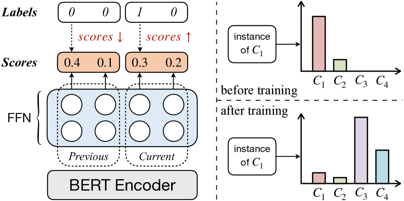
• classifier bias: without the previous training data, the class weights of previous relations would be improperly updated, leading to a skewed output distribution as shown in Figure 1.

• representation bias: the learned representations of current relations would be easily overlapped with those of previous relations in the representation space.

To alleviate the biases mentioned above, we propose a simple yet effective classifier decomposition framework inspired by Wang et al. (2021). The framework splits the last FFN layer into the separated previous and current classifiers, and introduces two enhanced strategies: empirical initialization and adversarial tuning. Specifically, To alleviate the classifier bias, empirical initialization firstly preserves the well-learned previous classifier nodes and then reuses them after learning current relations. To ease the representation bias, adversarial tuning slows down the update of previous classifier weights. The slowly updating weights can be seen as a series of adversarial signals that induce CRE models to learn distinguishable representations.

To sum up: (1) we find that CRE models suffer from classifier and representation biases when learning the new relations. (2) we propose a simple yet effective classifier decomposition framework with empirical initialization and adversarial tuning to alleviate these two biases. (3) Extensive experiments on FewRel and TACRED verify the effectiveness of our method.

2 Task Formalization

In CRE, models are trained on a sequence of tasks {$T_{1}$, $T_{2}$, …, $T_{k}$}, where the $k$-th task has its own training set $D_{k}=\{(x_{i},y_{i})\}_{i=1}^{N}$ with $C^{k}$ new relations. Each task $T_{k}$ is an independent supervised classification task to identify the instance $x_{i}$ (including the sentence and entity pair) into its corresponding relation label $y_{i}$. The goal of CRE is to learn new tasks while avoiding catastrophic forgetting of previously seen tasks. In other words, the model is evaluated to identify an instance into all $C^{k}_{prev}+C^{k}$ relations, where $C^{k}_{prev}=\sum_{i=1}^{k-1}C^{i}$ is the number of previously seen relations. To alleviate catastrophic forgetting in CRE, previous rehearsal-based work Han et al. (2020); Cui et al. (2021); Hu et al. (2022); Wang et al. (2022a) adopts an episodic memory module to store a few representative instances for each previous relation. In the subsequent training process, instances in the memory set will be replayed to balance the model’s performance on all seen relations.

FewRel
Models	T1	T2	T3	T4	T5	T6	T7	T8	T9	T10
EA-EMR Wang et al. (2019)	89.0	69.0	59.1	54.2	47.8	46.1	43.1	40.7	38.6	35.2
CML Wu et al. (2021)	91.2	74.8	68.2	58.2	53.7	50.4	47.8	44.4	43.1	39.7
RPCRE Cui et al. (2021)	97.9	92.7	91.6	89.2	88.4	86.8	85.1	84.1	82.2	81.5
EMAR† Han et al. (2020)	98.2	94.1	92.0	90.8	89.7	88.1	87.2	86.1	84.8	83.6
CRECL† Hu et al. (2022)	98.0	94.7	92.4	90.7	89.4	87.1	85.9	85.0	84.0	82.1
CRL Zhao et al. (2022)	98.1	94.6	92.5	90.5	89.4	87.9	86.9	85.6	84.5	83.1
Ours	98.2	94.9	93.2	91.9	91.3	89.6	88.3	87.1	86.0	84.6
w/ ACA Wang et al. (2022b)	98.4	95.4	93.2	92.1	91.0	89.7	88.3	87.4	86.4	84.8
TACRED
Models	T1	T2	T3	T4	T5	T6	T7	T8	T9	T10
EA-EMR Wang et al. (2019)	47.5	40.1	38.3	29.9	24.0	27.3	26.9	25.8	22.9	19.8
CML Wu et al. (2021)	57.2	51.4	41.3	39.3	35.9	28.9	27.3	26.9	24.8	23.4
RPCRE Cui et al. (2021)	97.6	90.6	86.1	82.4	79.8	77.2	75.1	73.7	72.4	72.4
EMAR† Han et al. (2020)	97.8	92.4	89.6	84.6	83.2	81.3	78.7	77.1	77.3	76.8
CRECL† Hu et al. (2022)	97.3	93.6	90.5	86.1	84.6	82.1	79.4	77.6	77.9	77.4
CRL Zhao et al. (2022)	97.7	93.2	89.8	84.7	84.1	81.3	80.2	79.1	79.0	78.0
Ours	97.9	93.1	90.1	85.8	84.7	82.6	81.0	79.6	79.5	78.6
w/ ACA Wang et al. (2022b)	97.7	92.8	91.0	86.7	85.2	82.9	80.8	80.2	78.8	78.6

Table 1: Accuracy (%) on all seen relations at the stage of learning current tasks. ^† denotes our reproduced results from open source code. Other results are directly taken from Zhao et al. (2022). We show the best results in boldface and the second best ones in underlines.

3 Methodology

The overall of our proposed classifier decomposition framework is illustrated in Figure 2. Following previous work Hu et al. (2022); Wang et al. (2022a); Zhao et al. (2022), our model architecture contains two main components: (1) an encoder that generates representations of a given instance and (2) a feed-forward network (FFN) that maps the encoded representation into a probability distribution over all seen relations.

3.1 Classifier Decomposition

To alleviate the illustrated two typical biases (i.e., classifier bias and representation bias) in the first training stage, we propose a classifier decomposition framework that splits the FFN layer into two independent groups of FFN nodes: the previous nodes and the current ones. The framework contains two enhanced strategies to alleviate the biases in stage 1, which include:

Empirical Initialization

Before the stage 1 training, we keep a frozen copy of the model’s previous FFN nodes, which represents the knowledge that the model learned in previous incremental tasks. This frozen copy is then utilized to initialize the parameters of the previous classifier before stage 2 so as to alleviate the classifier bias and retain the previous knowledge.

Adversarial Tuning

To alleviate the representation bias, we propose that the output distribution of previous relations is opposite to the optimization objective of the current task. This distribution can be viewed as adversarial signals, which helps the model learn more unique and distinguishable representations. Taking the analogous relation pair {$C_{1}$, $C_{n-1}$} (e.g., the relation pair of {“Mother”, “Father”}) in Figure 2 as an example, given a training instance of $C_{n-1}$, due to the high similarity of encoder representations between $C_{1}$ and $C_{n-1}$, the prediction score of $C_{1}$ will also be high. Thus, the training objective of current tasks will lead to two optimization paths: reduce the scores of $C_{1}$ or force the model to learn more unique representations of $C_{n-1}$. Inspired by this, we propose to slow down the update of previous classifier weights during training so as to steer the learning more toward the second optimization path. Formally,

$$\theta_{prev}\leftarrow\theta_{prev}-\alpha_{prev}\frac{\partial}{\partial\theta_{prev}}\mathcal{L}$$ (1)

$$\theta_{cur}\leftarrow\theta_{cur}-\alpha_{cur}\frac{\partial}{\partial\theta_{cur}}\mathcal{L}$$ (2)

where $\alpha_{prev}$, $\alpha_{cur}$ are the learning rate of the previous and current output embeddings, respectively. We adopt a lower $\alpha_{prev}$ in the training of stage 1.

3.2 Training and Inference

Following previous work Han et al. (2020); Cui et al. (2021); Hu et al. (2022); Wang et al. (2022a), the training loss function at task $T_{k}$ of our framework is given by:

$$\mathcal{L}=\sum_{i=1}^{D^{*}}-\log P(y_{i}|x_{i})$$ (3)

where $P(y_{i}|x_{i})$ is the prediction scores calculated by the FFN layer, $(x_{i},y_{i})$ is the sample from $D^{*}$, $D^{*}$ denotes $D_{k}$ in stage 1 or the memory set in stage 2. Specifically, $P(y_{i}|x_{i})$ is given by:

$$P(y_{i}|x_{i})={\rm softmax}(\mathbf{W}\mathbf{h})$$ (4)

where $\mathbf{h}\in\mathbb{R}^{d}$ is the encoder representation of the instance $x_{i}$; $\mathbf{W}\in\mathbb{R}^{d\times(C_{prev}^{k}+C^{k}})$ stands for the weights of the FFN layer. During inference, we select the relation with the max prediction score as the predicted relation.

4 Experiments

4.1 Experimental Setups

Datasets

Following previous work Han et al. (2020); Cui et al. (2021); Hu et al. (2022); Wang et al. (2022a), our experiments are conducted upon two standard benchmarks, FewRel Han et al. (2018) and TACRED Zhang et al. (2017), please refer to Appendix A.1 for more details.

Implement Details

For fair comparisons, we use the same experimental settings as Cui et al. (2021); Zhao et al. (2022), which randomly divide all relations into 10 sets to simulate 10 tasks and report the average accuracy of 5 different sampling task sequences. The number of stored instances in the memory for each relation is $10$ for all methods. We adopt the same random seeds to guarantee that the task sequences are exactly the same. We search the learning rate $\alpha_{prev}\in[0,1e-6,1e-5,1e-4]$ for the previous classifier in adversarial tuning. More details of our experimental settings and comparison baselines are included in Appendix A.2 and A.3.

Figure 3: F1 scores of previous relations in the training of stage 1. Results are obtained on the FewRel dataset.

4.2 Main Results

The performances of our proposed classifier decomposition framework and baselines on two datasets are shown in Table 1. The results indicate that our framework is significantly superior to other baselines ($p<0.05$) and achieves state-of-the-art performance in the vast majority of settings. Besides, this framework is orthogonal to the data augmentation strategy proposed by Wang et al. (2022b), which can further boost the model’s performance.

4.3 Analysis

Effectiveness of Empirical Initialization

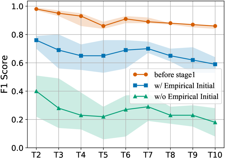
As shown in Figure 3, after stage 1, the model’s performance on previous relations is consistently improved with our proposed empirical initialization strategy on all tasks, which indicates that the bias in previous relations is effectively alleviated.

Figure 4: The instance representations belonging to P25 (“mother”) and P26 (“spouse”) after learning P25 and P26, respectively.

Effectiveness of Adversarial Tuning

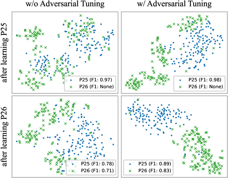
We utilize t-SNE to visualize the representations of a analogous relation pair: P25 (“mother”) and P26 (“spouse”). As shown in Figure 4, with adversarial tuning, the representations of instances belonging to P25 and P26 is much more separable compared with those of the vanilla training strategy, which indicates that adversarial tuning indeed alleviates the representation bias and helps the model learn more robust representations.

Models	FewRel	TACRED
Ours	84.6	78.6
w/o Empirical Initialization	84.3	78.4
w/o Adversarial Tuning	84.0	77.9
w/o both	83.5	77.6

Table 2: Accuracy (%) of models with different strategies.

Ablation Study

We further conduct an ablation study of our proposed two enhanced strategies in Table 2. The experimental results show a performance degradation with the ablation of both strategies, demonstrating the effectiveness of our proposed classifier decomposition framework.

5 Conclusion

In this work, we found that the vanilla training strategy adopted by most previous CRE models in the first training stage leads to two typical biases: classifier bias and representation bias, which are important factors causing catastrophic forgetting. To this end, we propose a simple yet effective classifier decomposition framework with two enhanced strategies to help models alleviate those biases at the first training stage. Experimental results on two benchmarks show that our framework consistently outperforms previous state-of-the-art CRE models, which indicates that the value of this training stage to CRE models may be undervalued. Further analysis shows the effectiveness of our proposed classifier decomposition framework.

Limitations

As a preliminary study, our proposed classifier decomposition framework focuses on the first training stage of CRE models with a lack of explorations on stage 2. Besides, more experiments can be conducted by combining our framework with previous leading CRE models, which we leave for future research. In addition, our work only focuses on strategies with the FFN layer. As the BERT encoder is the main component of CRE models, we call for more attentions to the research of improving encoder representations in the first training stage.

Appendix A Experiments Details

A.1 Datasets

Following previous work Han et al. (2020); Cui et al. (2021); Hu et al. (2022); Wang et al. (2022a), our experiments are conducted upon the following two standard benchmarks with the training-test-validation split ratio set to 3:1:1.

FewRel

Han et al. (2018) It is a RE benchmark dataset originally proposed for few-shot learning. The dataset contains 100 relations, each with 700 instances. Following the previous work Wang et al. (2019); Han et al. (2020); Zhao et al. (2022), we use the original training and validation set of FewRel, which contains 80 relations.

TACRED

Zhang et al. (2017) It is a large-scale RE dataset containing 42 relations (including no_relation) and 106,264 samples, which is constructed on news networks and online documents. Following Cui et al. (2021), we removed no_relation in our experiments. The number of training samples for each relation is limited to 320 and the number of test samples of relation to 40.

A.2 Experimental Details

Following previous work Han et al. (2020); Cui et al. (2021), we use bert-base-uncased as our encoder and Adam as our optimizer. We set the learning rate $1e-3$ for non-BERT modules and $1e-5$ for the BERT module, if not specified. The batch size of training is 32. The memory size of each task is 10. The training epoch for stage 1 and stage 2 are set to 10 for FewRel and 8 for TACRED. Our experiments are conducted on a single NVIDIA 3090 GPU.

A.3 Baselines

We compare our proposed framework with the following baselines in our experiments:

• EA-EMR Wang et al. (2019) proposes a memory replay and embedding alignment mechanism to alleviate the problem of catastrophic forgetting.

• EMAR Han et al. (2020) constructs a memory activation and reconsolidation mechanism to alleviate the catastrophic forgetting.

• CML Wu et al. (2021) introduces curriculum learning and meta-learn to alleviate order sensitivity and catastrophic forgetting in CRE.

• RPCRE Cui et al. (2021) proposes relation prototypes and a memory network to refine sample embeddings, which effectively retains the learned representations in CRE;

• CRL Zhao et al. (2022) proposes to utilize contrastive learning and knowledge distillation to alleviate catastrophic forgetting.

• CRECL Hu et al. (2022) introduces prototypical contrastive learning to ensure that data distributions of all CRE tasks are more distinguishable to alleviate catastrophic forgetting.

Appendix B Learning rate in Adversarial Tuning

We search various learning rates for previous classifier in adversarial tuning. The results shown in Table 3 indicate that the rate of $1e-5$ performs best, which is on par with that of the BERT encoder. It is worth noting that completely freezing the previous classifier (i.e., $lr=0$) leads to performance degradation since the model easily overfits on the fixed output distribution of the previous classifier.

Learning Rate	$0$	$1e-6$	$1e-5$	$1e-4$
FewRel	82.2	84.0	84.6	83.9
TACRED	76.5	77.8	78.6	78.0

Table 3: Accuracy (%) of models with various learning rates.

Appendix C Case Study

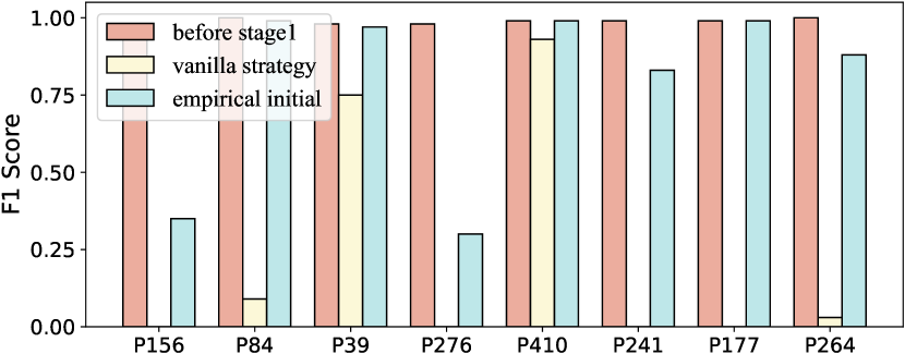
We show a specific case including F1 scores of previous relations after the first training stage of the task $T_{2}$. As shown in Figure 5, significant improvement in scores of previous relations is shown with the empirical initialization strategy, indicating its effectiveness.

Figure 5: A case of empirical initialization on the FewRel dataset.

Appendix D Representations with Adversarial Tuning

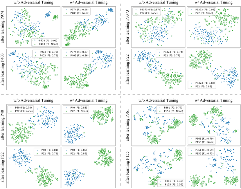
We illustrate more cases in Figure 6 to show the effectiveness of adversarial tuning strategy.

Figure 6: More cases of robust representation learning with adversarial tuning.

References

- Cui et al. (2021) Li Cui, Deqing Yang, Jiaxin Yu, Chengwei Hu, Jiayang Cheng, Jingjie Yi, and Yanghua Xiao. 2021. Refining sample embeddings with relation prototypes to enhance continual relation extraction. In Proceedings of the 59th Annual Meeting of the Association for Computational Linguistics and the 11th International Joint Conference on Natural Language Processing, ACL/IJCNLP 2021, (Volume 1: Long Papers), Virtual Event, August 1-6, 2021, pages 232–243. Association for Computational Linguistics.
- Han et al. (2020) Xu Han, Yi Dai, Tianyu Gao, Yankai Lin, Zhiyuan Liu, Peng Li, Maosong Sun, and Jie Zhou. 2020. Continual relation learning via episodic memory activation and reconsolidation. In Proceedings of the 58th Annual Meeting of the Association for Computational Linguistics, ACL 2020, Online, July 5-10, 2020, pages 6429–6440. Association for Computational Linguistics.
- Han et al. (2018) Xu Han, Hao Zhu, Pengfei Yu, Ziyun Wang, Yuan Yao, Zhiyuan Liu, and Maosong Sun. 2018. Fewrel: A large-scale supervised few-shot relation classification dataset with state-of-the-art evaluation. In Proceedings of the 2018 Conference on Empirical Methods in Natural Language Processing, Brussels, Belgium, October 31 - November 4, 2018, pages 4803–4809. Association for Computational Linguistics.
- Hu et al. (2022) Chengwei Hu, Deqing Yang, Haoliang Jin, Zhen Chen, and Yanghua Xiao. 2022. Improving continual relation extraction through prototypical contrastive learning. In Proceedings of the 29th International Conference on Computational Linguistics, COLING 2022, Gyeongju, Republic of Korea, October 12-17, 2022, pages 1885–1895. International Committee on Computational Linguistics.
- Wang et al. (2019) Hong Wang, Wenhan Xiong, Mo Yu, Xiaoxiao Guo, Shiyu Chang, and William Yang Wang. 2019. Sentence embedding alignment for lifelong relation extraction. In Proceedings of the 2019 Conference of the North American Chapter of the Association for Computational Linguistics: Human Language Technologies, NAACL-HLT 2019, Minneapolis, MN, USA, June 2-7, 2019, Volume 1 (Long and Short Papers), pages 796–806. Association for Computational Linguistics.
- Wang et al. (2022a) Peiyi Wang, Yifan Song, Tianyu Liu, Rundong Gao, Binghuai Lin, Yunbo Cao, and Zhifang Sui. 2022a. Less is more: Rethinking state-of-the-art continual relation extraction models with a frustratingly easy but effective approach. CoRR, abs/2209.00243.
- Wang et al. (2022b) Peiyi Wang, Yifan Song, Tianyu Liu, Binghuai Lin, Yunbo Cao, Sujian Li, and Zhifang Sui. 2022b. Learning robust representations for continual relation extraction via adversarial class augmentation. CoRR, abs/2210.04497.
- Wang et al. (2021) Peiyi Wang, Runxin Xun, Tianyu Liu, Damai Dai, Baobao Chang, and Zhifang Sui. 2021. Behind the scenes: An exploration of trigger biases problem in few-shot event classification. In Proceedings of the 30th ACM International Conference on Information & Knowledge Management, pages 1969–1978.
- Wu et al. (2021) Tongtong Wu, Xuekai Li, Yuan-Fang Li, Gholamreza Haffari, Guilin Qi, Yujin Zhu, and Guoqiang Xu. 2021. Curriculum-meta learning for order-robust continual relation extraction. In Thirty-Fifth AAAI Conference on Artificial Intelligence, AAAI 2021, Thirty-Third Conference on Innovative Applications of Artificial Intelligence, IAAI 2021, The Eleventh Symposium on Educational Advances in Artificial Intelligence, EAAI 2021, Virtual Event, February 2-9, 2021, pages 10363–10369. AAAI Press.
- Zhang et al. (2017) Yuhao Zhang, Victor Zhong, Danqi Chen, Gabor Angeli, and Christopher D. Manning. 2017. Position-aware attention and supervised data improve slot filling. In Proceedings of the 2017 Conference on Empirical Methods in Natural Language Processing, EMNLP 2017, Copenhagen, Denmark, September 9-11, 2017, pages 35–45. Association for Computational Linguistics.
- Zhao et al. (2022) Kang Zhao, Hua Xu, Jiangong Yang, and Kai Gao. 2022. Consistent representation learning for continual relation extraction. In Findings of the Association for Computational Linguistics: ACL 2022, Dublin, Ireland, May 22-27, 2022, pages 3402–3411. Association for Computational Linguistics.