Flex-SFU: Accelerating DNN Activation Functions by Non-Uniform Piecewise Approximation

Abstract

Modern DNN workloads increasingly rely on activation functions consisting of computationally complex operations. This poses a challenge to current accelerators optimized for convolutions and matrix-matrix multiplications. This work presents Flex-SFU, a lightweight hardware accelerator for activation functions implementing non-uniform piecewise interpolation supporting multiple data formats. Non-Uniform segments and floating-point numbers are enabled by implementing a binary-tree comparison within the address decoding unit. An SGD-based optimization algorithm with heuristics is proposed to find the interpolation function reducing the mean squared error. Thanks to non-uniform interpolation and floating-point support, Flex-SFU achieves on average 22.3x better mean squared error compared to previous piecewise linear interpolation approaches. The evaluation with more than 700 computer vision and natural language processing models shows that Flex-SFU can, on average, improve the end-to-end performance of state-of-the-art AI hardware accelerators by 35.7%, achieving up to 3.3x speedup with negligible impact in the models’ accuracy when using 32 segments, and only introducing an area and power overhead of 5.9% and 0.8% relative to the baseline vector processing unit.

I Introduction

To keep pace with the evolution of artificial intelligence (AI) models, industry and academia are exploring novel hardware architectures, featuring heterogeneous processing units capable of achieving orders of magnitude improvements in terms of performance and energy efficiency with respect to general-purpose processors. As the execution time of state-of-the-art deep neural networks (DNNs) has been dominated by operations like convolutions and matrix-multiplications [1, 2], DNN hardware accelerators currently allocate most of their computational resources to specialized linear algebra cores, while leaving the execution of the other layers to general-purpose vector processing units (VPUs) [3, 4]. However, aiming at reducing training and inference time and enabling deployment on IoT and edge devices, recent deep learning research efforts are pushing towards decreasing the models’ dimension while providing comparable or better accuracy. To this aim, recent networks increase their heterogeneity by introducing new layers featuring reduced operational intensity and new parameter-free layers. As these new layers can be efficiently computed by exploiting highly data-parallel accelerators, they are significantly increasing the share of execution time spent on the VPUs hosted in DNN hardware accelerators. Specifically, parameter-free layers like the rectified linear unit (ReLU) are increasingly replaced with activation functions requiring a higher compute effort, such as the Gaussian error linear unit (GELU), the sigmoid linear unit (SiLU), and Softmax, which are composed of several expensive operations like divisions and exponentiations [5]. This trend can be seen clearly in Figure 1, analyzing the activation functions distribution over the past years, considering $628$ computer vision DNNs and $150$ natural language processing (NLP) transformers from PyTorch Image Models (TIMM) [6] and Hugging Face [7], respectively. While ReLU was the dominant activation function from 2015 to 2017, it declined to $20.7\%$ in 2021, while functions like SiLU and GELU emerged over the last years, jointly accounting for $32.1\%$ and $44.2\%$ of the total activation functions count in 2020 and 2021, and requiring $4\times$ and $12\times$ more arithmetic operations than ReLU, respectively. Therefore, exploring novel hardware architectures capable of efficiently accelerating the computation of complex activation functions is becoming an increasingly important research topic.

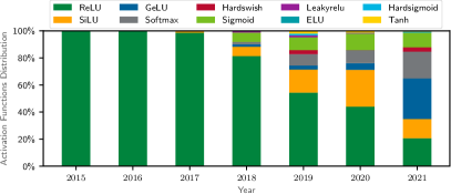
Figure 1: Activation functions distribution by year of model publication, extracted from 700+ SoA AI models of the TIMM and Hugging Face collections [6, 7].

In this paper, we propose Flex-SFU, a flexible hardware accelerator for deep learning activation functions, integrated in general-purpose VPUs and relying on a novel piecewise linear (PWL) approximation approach, capable of averagely improving the precision of previous PWL approximation approaches by $22.3\times$. The main novelty of Flex-SFU relies on its flexibility. Indeed, its functionality can be reprogrammed to approximate all common activation functions. It supports 8-, 16-, and 32-bit fixed-point and floating-point data formats, and it allows selecting arbitrary locations for the PWL interpolation points.

The main contributions of this paper are listed as follows:

• We propose a reprogrammable hardware architecture, extending the set of functional units hosted in VPUs, capable of improving the performance of activation functions computations and supporting both fixed-point and floating-point operations;

• We define a PWL algorithm to automatically find the best interpolation points of any DNN activation function, supporting arbitrary positions of the interpolation points and achieving negligible top-1 accuracy drops on the analyzed models considering 16 or 32 breakpoints;

• An end-to-end performance and accuracy evaluation of Flex-SFU, targeting a commercial DNN accelerator and benchmarking more than 700 SoA deep learning models.

II Background and Motivation

Activation functions represent one of the most common and important layers of DNNs, as they apply non-linear transformations to the network feature maps. While ReLU has been widely used for many deep learning tasks, modern networks are using more complex activation functions [8] to achieve higher accuracies and avoid the well-known “dying ReLU effect” [9]. As these kernels require many complex operations, they are typically accelerated via function approximation strategies, whose methods can be grouped into three main categories: polynomial, lookup table (LUT)-based, and hybrid.

Polynomial approximation methods [10, 11] compute the activation functions through series expansions, such as Taylor and Chebyshev approximations. Although these methods feature high-precision computations, their hardware implementations are typically tailored to a specific activation function and are costly in terms of area, as their computation requires several multiply-add (MADD) operations.

LUT-based architectures [12, 13, 14, 15] feature higher flexibility than polynomial methods. They perform a PWL approximation, subdividing the function input range into intervals and associating each interval to a specific function output, whose value is pre-computed and stored in memories used as LUTs. An addressing scheme is then used to map a given input [13] or a full interval [14] to a specific LUT address, holding the corresponding function output. LUT-based solutions can be more flexible than polynomial methods, as programmable LUTs can store different sets of output data depending on the target activation function. However, they require a high area footprint to provide good accuracy. Indeed, as the function output is directly provided by the LUT, the approximation precision strictly depends on the number of intervals (i.e., the LUT depth) in a selected input range.

To overcome these limitations, several works [16, 17, 18, 19, 20] explore hybrid solutions, which combine the polynomial and LUT-based approaches by storing in the LUTs the interpolation segment coefficients instead of the function outputs. For example, a PWL hybrid approach approximates a given activation function as $N$ straight lines (i.e., segments), each satisfying the equation $f(x)=m_{i}x+q_{i}$, for $i\in\{0,1,...,N-1\}$. A MADD operation is then used to compute the function output (i.e., f(x)) starting from a specific set of segment coefficients stored in the LUTs (i.e., $m_{i}$, $q_{i}$) and from the incoming input data (i.e., x).

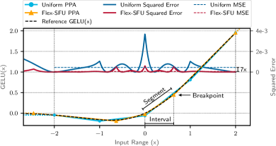
Figure 2: PWL approximation (left y-axis) and squared error (right y-axis) of GELU, exploiting uniform and non-uniform (i.e., Flex-SFU) interpolations, and considering 5 breakpoints (i.e., 4 segments) in the [-2,2] input range.

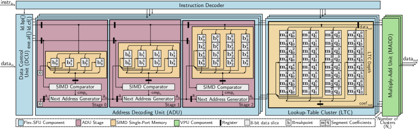
Figure 3: Flex-SFU hardware architecture, integrated into the main VPU as an additional functional unit, considering Look-up table clusters (LTCs) capable of storing 8 segment coefficients. Memory cell superscripts represent breakpoints and coefficients IDs, while memory cell subscripts represent data slices.

Hybrid solutions outperform LUT-based approaches in terms of area and accuracy, as they are able to correctly approximate the whole segment instead of selecting a reference output value for a given interval. Moreover, hybrid approaches relax the constraint on the maximum function input range, as they allow to approximate any function featuring boundaries that converge to a fixed slope.

However, current hybrid solutions present several limitations. ❶ They are tailored to a single input data type, either converted into a fixed-width fixed-point notation [16, 17, 18, 21] or only considering a single floating-point format [19, 20]. Moreover, their LUT addressing schemes simply rely on a fixed subset of bits, such as the input data most significant bits (MSBs). However, these approaches lack flexibility, firstly because current accelerators support several data formats and single instruction multiple data (SIMD) computations [22], (e.g., from four 8-bit to one 32-bit elements/cycle), and secondly because their addressing schemes need to be tailored for each target function and input data type. ❷ Their approximation methods mainly rely on uniform interpolations (i.e., segments share the same length). However, activation function approximations would benefit from non-uniform interpolation granularity among different function intervals, as it would allow increasing the density of segments on more sensitive intervals while relaxing their density on straight intervals. For example, in Figure 2, showing the PWL approximation of GELU exploiting both uniform and non-uniform interpolations, the non-uniform strategy improves the mean squared error (MSE) by $7\times$ while using the same number of breakpoints. Although non-uniform strategies exist in the literature, they either rely on simply removing breakpoints from a uniform interpolation while maintaining similar precisions [23, 24], or only optimize the interpolation error for narrow input ranges, leaving it diverging outside the selected interval with unknown impact on the end-to-end accuracy [21]. ❸ Although many related works[17, 18, 19, 20] perform end-to-end accuracy evaluations on selected deep learning models, none of them quantify the accuracy impact of their solutions on a large set of networks. However, such analyses are crucial to verify the robustness of a given approximation method, as different models can suffer from varying sensitivities to activation function errors.

To overcome these limitations, we propose Flex-SFU, whose hardware architecture (detailed in Section III) supports all the data sizes typically used by DNNs, and features linear throughput scaling with constant on-chip memory usage. Our reprogrammable hardware architecture implements an addressing scheme supporting non-uniform segments, whose optimal lengths minimizing the approximation MSE are determined by a novel PWL algorithm, described in Section IV.

III Flex-SFU Hardware Architecture

The proposed hardware architecture implements a hybrid PWL approach to approximate activation functions. It supports both fixed-point and floating-point data formats composed of 8-, 16-, and 32-bit, representing the most used data types targeting deep learning applications.

Depending on the input data value, Flex-SFU provides the proper coefficients to the VPU MADD units, computing the activation function output. Differently from the related work analyzed in Section II, performing the address decoding exploiting a subset of incoming input data bits, Flex-SFU relies on small memories to store the breakpoint values on-chip, and compares them with the incoming data to find the respective LUT address. This feature allows for higher flexibility than solutions only supporting uniform segments, as it permits to select the best length for each segment, thus minimizing the approximation error.

Flex-SFU extends the set of functional units available on current VPUs targeting deep learning, acting as a special function unit (SFU) capable of accelerating activation functions via PWL approximation. Its execution is handled by three custom instructions extending the target VPU instruction set architecture (ISA), namely ld.bp(), ld.cf(), and exe.af(). The proposed instructions are decoded by the VPU, and then handled by Flex-SFU, whose main architectural components are depicted in Figure 3. A data control unit (DCU) dispatches input data among the other Flex-SFU units. Specifically, ld.bp() and ld.cf() source data, holding either breakpoints or PWL coefficients, are sent by the DCU to the address decoding unit (ADU) or the lookup table cluster (LTC) unit, and stored in SIMD single-port memories. These instructions must be executed only once when a different activation function has to be computed, and can be pre-executed while other accelerator compute units (e.g., the main tensor-unit) are still computing the activation function inputs. Therefore, as discussed in Section V-A, they do not introduce a large overhead in the overall computation. Once breakpoints and LUT coefficients have been loaded in the ADU and LTC units, multiple exe.af() can be executed to compute the activation function outputs. These operations are handled by the DCU, which streams the input data through the pipeline composed of the ADU and the LTC. As Figure 3 shows, the ADU functionality resembles a binary search tree (BST). Each ADU stage defines a BST level, and exploits SIMD single-port memories to implement BST nodes holding breakpoints, which are ordered to allow traversing one BST level per stage to search for the proper LTC address depending on the input data. Each cycle, a SIMD comparator supporting both fixed-point and floating-point number formats determines if the current input data is greater or smaller than the breakpoint loaded from memory exploiting the cmp_o signal, whose value can be either 1 or 0, respectively. The comparison output and the input address are then used by the Next Address Generator unit to find the subsequent ADU stage address, namely $a_{o}$. The last ADU stage performs the comparison among the BST leaves, thus finding the proper LUT address which is forwarded to the LTC unit. Finally, the LTC loads the appropriate segment coefficients, and sends them and the delayed input data to the VPU MADD functional units, computing the activation function output.

The memory-mapping strategy exploited by the ADU and LTC units consists of four SIMD single-port memories, whose bit-width is equal to the product between the minimum supported bit-width (i.e., 8-bit) and the number of coefficients (i.e., 1 and 2 for the ADU and LTC, respectively). Each memory is accessed separately in case of computations based on 8-bit data (e.g., $b^{i}_{0}$, $b^{i}_{1}$, $b^{i}_{2}$, $b^{i}_{3}$ are accessed as four separate 8-bit data), while for 16-bit computations each data is segmented among two subsequent memories (e.g., $b^{i}_{0}$ - $b^{i}_{1}$ and $b^{i}_{2}$ - $b^{i}_{3}$ are accessed as two 16-bit data), in such a way to support an input throughput of two 16-bit elements/cycle. Similarly, the same data is partitioned among the four 8-bit memories in case of 32-bit computations (e.g., $b^{i}_{0}$ - $b^{i}_{1}$ - $b^{i}_{2}$ - $b^{i}_{3}$ are accessed as a single 32-bit data), allowing to support a throughput of one 32-bit element/cycle, while reusing the same memories.

As shown in Figure 3, to allow for further scalability, the Flex-SFU parallelism can be tuned by increasing the number of instantiated clusters, namely N_c, to match the underlying VPU throughput. Note that, as VPUs are typically optimized for throughput, we design Flex-SFU exploiting pipelining, thus enabling steady-state performance of N_c $\times$ 32-bit/cycle, while avoiding dead-locks by design.

IV Flex-SFU Approximation Methodology

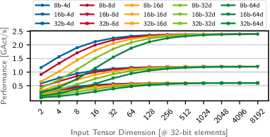
Figure 4: Throughput of Flex-SFU, in terms of number of computed activations (i.e., GAct) per second, as a function of the input tensor size, accounting for different bit-widths (b) and lookup table cluster (LTC) depths (d)

We rely on a PWL approximation, defining the interpolated and steady function $\hat{f}(x)$ as:

$$f(x)\approx\hat{f}(x)=\begin{cases}m_{l}(x-p_{0})+v_{0}&x\leq p_{0}\\ \frac{v_{i+1}-v_{i}}{p_{i+1}-p_{i}}(x-p_{i})+v_{i}&p_{i}<x<p_{i+1},\\ &0<i<n-1\\ m_{r}(x-p_{n-1})+v_{n-1}&x\geq p_{n-1}\end{cases}$$

with $n$ breakpoints $p_{i}$, $(n+1)$ linear segments, and $n$ function values at the breakpoints $v_{i}=\hat{f}(p_{i})$. The most left and right segments are calculated with values $v_{0}$ and $v_{n+1}$, using slopes $m_{l}$ and $m_{r}$, while the inner segments of each breakpoint $p_{i}$ are linearly interpolated through its value $v_{i}$ and the following breakpoint-value pair [$p_{i+1}$;$v_{i+1}$].

To find the breakpoint-value pairs, we start with uniformly distributed breakpoints and exact function values. We use the Adam optimizer [25] (with lr=0.1, momenta=(0.9, 0.999)) and the Plateau LR scheduler. We choose the MSE between the interpolated function $\hat{f}$ and the target function $f$ on the interval $[a,b]$ as the loss function:

$$\mathcal{L}_{[a,b]}(\hat{f},f)=\frac{1}{b-a}\int_{a}^{b}(\hat{f}(x)-f(x))^{2}dx$$

Aiming to avoid stalls in sub-optimal local minima during the optimization process, we extend our optimization algorithm by removing breakpoints and reinserting them at a better location.

Removal loss: We define the removal loss $\ell_{i}^{\text{rm}}$ as the loss of the interpolated function if the breakpoint $p_{i}$ is removed. We then remove the breakpoint with the minimal removal loss, $p_{\mathrm{remove}}$:

$$p_{\mathrm{remove}}=\operatorname*{arg\;min}_{p_{i}}\;\ell_{i}^{\text{rm}},\qquad\ell_{i}^{\text{rm}}=\mathcal{L}_{[a,b]}(\hat{f}_{{\{p_{j},v_{j}\}}_{j\neq i}},f).$$

Insertion loss: On the other hand, we define the insertion loss $\ell_{i}^{\text{ins}}$ as the loss over the $i$-th segment, and insert a new breakpoint in the center of the segment with the highest insertion loss:

$$\begin{pmatrix}p_{\mathrm{insert}}\\ v_{\mathrm{insert}}\end{pmatrix}=\operatorname*{arg\;max}_{\scriptsize\begin{pmatrix}(p_{i}+p_{i+1})/2\\ (v_{i}+v_{i+1})/2\end{pmatrix}}\ell_{i}^{\text{ins}},\ \ell_{i}^{\text{ins}}=(p_{i+1}-p_{i})\mathcal{L}_{[p_{i},p_{i+1}]}(\hat{f},f).$$

Boundary condition: All relevant activation functions converge outside the interpolation interval to a constant value or an asymptote. To avoid large errors outside of the interpolation interval, unless noted otherwise, we define boundary conditions for value and slope for the most left and the most right segments, such that they lie on the asymptote of the function:

$$m_{l} =\lim_{x\to-\infty}f(x)/x, v_{0} =m_{l}p_{0}+\lim_{x\to-\infty}(f(x)-m_{l}x)\mathrm{,}$$

$$m_{r} =\lim_{x\to+\infty}f(x)/x, v_{n-1} =m_{r}p_{n-1}+\lim_{x\to+\infty}(f(x)-m_{r}x)$$

For example, considering GELU, this resolves to $m_{l}=0,v_{0}=0,m_{r}=1,v_{n-1}=p_{n-1}$. Notably, $p_{0}$ and $p_{n-1}$ themselves are still learned. In this way, the interpolated function converges to the original function for values far from the boundary breakpoints. This comes at a small cost in error close to the boundary breakpoints.

Optimization strategy: We initialize the Flex-SFU function interpolation with uniformly distributed breakpoints. Then we optimize with SGD until convergence. After this, we remove and insert one breakpoint as described above, and retrain with a lower learning rate. We reiterate until removal and insertion points converge. Note that we perform this optimization for each function, and we substitute the layers within the DNN models without any retraining for ease of use.

TABLE I: Flex-SFU Characterization for N_c = 1 at $f=600$ MHz in 28nm CMOS

LTC Depth (i.e., # Segments)	4	8	16	32	64
Latency [cycles]	7	8	9	10	11
Power [mW]	1.4	1.7	2.2	2.8	3.7
ADU Area [%]	34.2%	41.2%	43.7%	46.0%	41.6%
LTC Area [%]	31.3%	34.9%	44.1%	46.6%	53.4%
Total Area [µm2]	2572.4	3593.0	5846.0	9791.3	14857.2

V Experimental Evaluation

V-A Performance, Power and Area Analyses

We implement the proposed hardware accelerator in register transfer level (RTL), and perform synthesis and place-and-route (PnR) for a 28nm CMOS technology node. We evaluate several Flex-SFU configurations in terms of performance, area, and power, varying the number of segments from 4 to 64 while considering $N_{c}=1$ and a target frequency of 600 MHz. Figure 4 shows the throughput of Flex-SFU, accounting for the time spent on both ld.bp(), ld.cf(), and exe.af(), across input tensors ranging from 2 to 8k 32-bit data. All the analyzed Flex-SFU combinations reach the steady-state performance for input tensors larger than 256 32-bit data, gaining 0.6 GAct/s, 1.2 GAct/s, and 2.4 GAct/s in terms of throughput, considering 8-, 16-, and 32-bit data sizes, corresponding to an energy efficiency ranging from 158 GAct/s/W to 1722 GAct/s/W. Note that the throughput reported in Figure 4 saturates to 1 OP/cycle, 2 OP/cycle, and 4 OP/cycle for 32-, 16-, and 8-bit data sizes at 600 MHz, proving that Flex-SFU can reach the theoretical peak performance discussed in Section III, accelerating complex DNN activation functions exploiting the same computation time typically required by simple operations like ReLU.

Table I details the characterization of Flex-SFU, obtained after the PnR step and considering from 4 to 64 segments, reporting a total power consumption ranging from 1.4 mW to 3.7 mW, and a total area requiring from 2572 µm² to 14857 µm².

To investigate the area and power impact of Flex-SFU on high-performance VPUs, we perform a back-of-the-envelope integration of Flex-SFU into the RISC-V VPU proposed by Perotti et al. in [26], composed of 4 lanes and supporting a maximum data size of 64-bit. Our evaluation, considering four Flex-SFU instances (i.e., one instance per lane) featuring $N_{c}=2$ (i.e., supporting from $1\times$64-bit to $8\times$8-bit elements/cycle), shows that Flex-SFU only accounts for 2.2%, 3.5% and 5.9% of the total area for a LTC depth of 8, 16 and 32 elements, respectively, while consuming from 0.5% to 0.8% of the total power.

V-B Function Approximation Precision Analysis

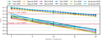
Figure 5: Error analysis for a set of activation functions, considering from 4 to 64 breakpoints. Interpolation intervals are in range [-10, 0.1] for the exponential function (Exp), and in range [-8, 8] for the other functions.

In Figure 5, we investigate MSE and maximum absolute error (MAE) of the most representative activation functions. We select the interpolation interval within [-10,0.1] for Exp, and within [-8,8] for the other functions. The boundary breakpoints lie on the functions’ asymptote to reduce the error outside the interpolation interval. We interpolate Exp for negative values to be used in Softmax, typically requiring exponentiation implemented with (vector-wide) maximum subtraction (i.e., $\exp(x_{i}-\max_{j}\;x_{j})$). As detailed in Figure 5, the approximation precision of the analyzed functions averagely improves MSE and MAE by $15.9\times$ and $3.8\times$ per doubling of the number of breakpoints. Moreover, all the interpolations featuring more than 16 breakpoints reach a MSE lower than 1 Float16 unit of least precision (ULP), defined as the single-bit error at a base of 1.

In Table II, we compare Flex-SFU with other PWL interpolation methods, considering the same interpolation range and number of breakpoints. Following most of the previous works, [16, 17, 18, 19, 20], we evaluate Flex-SFU exploiting the average absolute error (AAE) metric, squaring it (i.e., sq-AAE) to match the same MSE order of magnitude. Furthermore, we compare with the equivalent number of breakpoints of previous works exploiting symmetry [16, 12]. As Table II shows, our method outperforms all the other PWL approaches, by a factor ranging from 2.3$\times$ to 88.4$\times$, with an average of 22.3$\times$.

The method proposed by Gonzalez et al. [19] exploits a second-order piecewise but not-steady interpolation, averagely achieving $4.3\times$ better MSEs than Flex-SFU on Tanh, Sigmoid, and SiLU. Although Flex-SFU can be easily extended to support a second-order interpolation, we believe that the PWL methodology of Flex-SFU represents a better candidate to compute activation functions on DNN accelerators. Indeed, second-order approximations feature high area overheads, requiring to double the number of VPU MADD units to guarantee the same throughput of the proposed solution, as well as larger LUTs able to store an additional interpolation coefficient.

TABLE II: Comparison of our MSE-optimized method with other PWL Interpolation Methods with the same number of breakpoints and range

	Parameters			Error sq-AAE*
	Funct.	Range	#BP	Ref.	This work	Impr.
[16]	Tanh	[-8, 8]	16†	$5.76\cdot 10^{-6}$	$4.27\cdot 10^{-7}$	13.5$\times$
[17]		[-3.5, 3.5]	16	$3.58\cdot 10^{-5}$	$1.52\cdot 10^{-6}$	23.5$\times$
[17]		[-3.5, 3.5]	64	$1.12\cdot 10^{-7}$	$7.88\cdot 10^{-9}$	14.2$\times$
[18]		[-8, 8]	16	$1.00\cdot 10^{-6}$	$4.26\cdot 10^{-7}$	2.3$\times$
[20]		[1/64, 4]	32	$5.94\cdot 10^{-7}$	$6.72\cdot 10^{-9}$	88.4$\times$
[12]		[-4, 4]	32†	$9.81\cdot 10^{-7}$‡	$1.13\cdot 10^{-8}$‡	86.8$\times$
[16]	Sigmoid	[-8, 8]	16†	$8.10\cdot 10^{-7}$	$1.21\cdot 10^{-7}$	6.7$\times$
[17]		[-7, 7]	16	$8.95\cdot 10^{-6}$	$4.97\cdot 10^{-7}$	18.0$\times$
[17]		[-7, 7]	64	$2.82\cdot 10^{-8}$	$2.38\cdot 10^{-9}$	11.9$\times$
[18]		[-8, 8]	16	$6.25\cdot 10^{-6}$	$2.88\cdot 10^{-7}$	21.7$\times$
[20]		[1/64, 4]	32	$1.41\cdot 10^{-7}$	$3.80\cdot 10^{-8}$	3.7$\times$
[12]		[-4, 4]	64†	$3.92\cdot 10^{-8}$‡	$2.38\cdot 10^{-9}$‡	9.3$\times$
[18]	GeLU	[-8, 8]	16	$6.76\cdot 10^{-6}$	$1.89\cdot 10^{-7}$	9.0$\times$

• SoA reports average absolute error (AAE).

• Numbers in MSE.

• Uses symmetry to halve the number of segments.

V-C End-to-End Evaluation

We evaluate Flex-SFU on a commercial Huawei Ascend 310P AI processor [27], exploiting a benchmark suite targeting $628$ computer vision and $150$ NLP networks from PyTorch Image Models (TIMM) and Hugging Face, respectively. This accelerator represents an ideal candidate to demonstrate the benefits that Flex-SFU can provide to SoA DNNs accelerators, as it hosts a specialized matrix multiplication unit computing up to 4096 MAC/cycle, and processes the DNN activation functions on a general-purpose high-performance VPU. To perform our performance evaluation, we convert each benchmark suite model from Pytorch 1.11 [28] to ONNX 1.12 [29] with opset version 13, and we replace each activation function of the resulting model graph with a custom ONNX operator, implementing a set of instructions supported by the Huawei Ascend ISA, and whose latency and throughput match the Flex-SFU metrics presented in Section V-A. Then, we compile both the baseline and the Flex-SFU-based ONNX models for the Ascend AI processor with Ascend Tensor Compiler (ATC) v5.1 and run them on the target accelerator to extract and compare their end-to-end inference run time. In our evaluation, we compute each model using all 8 cores of the Ascend 310P AI processor in parallel with batch size equal to 1, considering the average execution time between 10 subsequent inference runs.

Figure 6 summarizes the execution time improvements of the proposed benchmark suite when exploiting Flex-SFU, highlighting the reference family and most frequent activation function of each model. We obtained comparable performance results, not reported for space reasons, for batch sizes equal to 16, 32, and 128. As Figure 6 shows, Flex-SFU matches the performance of models primarily relying on lightweight activation functions (i.e., ReLU, Leaky ReLU), not introducing any overhead in their computation, and greatly improves the execution time of networks relying on more complex activation functions. Specifically, including the models based on ReLU, whose baseline execution time matches the Flex-SFU performance, Flex-SFU allows gaining $17.3\%$, $17.9\%$, $29.0\%$, and $45.1\%$ performance on ResNets, Vision Transformers, NLP Transformers, and EfficientNets models, while reaching $2.1\times$ more performance on DarkNets models. Overall, Flex-SFU reaches $22.8\%$ better performance on the considered model zoo computation, improving the execution time of models relying on complex activation functions by $35.7\%$ on average, and reaching a performance peak of $3.3\times$ on the computation of resnext26ts.

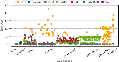
Figure 6: End-to-end model zoo performance evaluation on the Huawei Ascend 310P AI processor. Colors: Most frequently used activation function in DNN.

We evaluate the accuracy impact of Flex-SFU for DNNs in the TIMM database on the ImageNet dataset [30] by comparing the top-1 accuracy on the validation set between the reference model and one where the activations are replaced with Flex-SFU. Table III shows the percentage of networks featuring accuracy drops ranging from 0.1 % to 2 % with respect to the baseline accuracy, as well as the mean and maximum accuracy drops for 4 to 64 breakpoints. As Table III shows, while only a few networks can tolerate 4 breakpoints, 8 and 16 breakpoints already allow 80% and 90% of the networks to achieve a drop smaller than 0.1%, with a mean drop of 0.87% and 0.26%, respectively. Moreover, 32 and 64 breakpoints are almost lossless, with 99% and 100% of the models showing less than 0.1% drop, and featuring maximum accuracy penalties of 0.30% and 0.04%, respectively. We noted that networks using SiLU are the most sensitive to approximation. For example, to feature an accuracy drop smaller than 0.17%, mobilevit and halonet50ts require 32 breakpoints, while lambda_resnet50ts and mixer_b16_224_miil require 16 breakpoints. Hardswish is the second most sensitive activation function, with lcnet and mobilenetv3_small requiring 32 breakpoints, and hardcorenas, fbnet, and mobilenetv3_large requiring 16 breakpoints to show losses smaller than 0.15%. Finally, GELU-based sebotnet33ts_256, mixer and crossvit achieve lossless accuracy drops with 16 breakpoints.

VI Conclusion

We proposed Flex-SFU, a scalable hardware accelerator for DNN activation functions on VPUs based on a novel interpolation methodology supporting non-uniform breakpoints locations, and performing 8-, 16-, and 32-bit computations based on both fixed-point and floating-point data formats. Our evaluation shows that Flex-SFU features low area and power overheads, and reaches $22.3\times$ MSE improvements on average with respect to other SoA PWL approaches. Moreover, our end-to-end evaluation on more than 700 SoA DNNs shows that commercial DNN accelerators can benefit from Flex-SFU, allowing them to improve their inference performance up to $3.3\times$ while retaining the models’ accuracies.

TABLE III: End-to-End Accuracy Drop over 600 DNNs of TIMM[6]

	Models Distribution						Accuracy Drop
#BP	<0.1	<0.2	<0.5	<1	<2	>2	mean	max
4	0.51	0.52	0.54	0.56	0.58	0.42	-25.95	-87.00
8	0.80	0.84	0.89	0.92	0.95	0.05	-0.87	-77.58
16	0.90	0.93	0.95	0.97	0.98	0.02	-0.26	-25.79
32	0.99	1.00	1.00	1.00	1.00	0.00	0.00	-0.30
64	1.00	1.00	1.00	1.00	1.00	0.00	0.00	-0.04

References

- [1] K. He et al., “Deep residual learning for image recognition,” in IEEE CVPR, 2016.
- [2] K. Simonyan et al., “Very deep convolutional networks for large-scale image recognition,” arXiv, 2014.
- [3] N. P. Jouppi et al., “In-datacenter performance analysis of a tensor processing unit,” in IEEE ISCA, 2017.
- [4] H. Liao et al., “Davinci: A scalable architecture for neural network computing,” in IEEE Hot Chips 31 Symposium (HCS), 2019.
- [5] “A survey on modern trainable activation functions,” Neural Networks, 2021.
- [6] R. Wightman, “Pytorch image models,” https://github.com/rwightman/pytorch-image-models, 2019.
- [7] T. Wolf et al., “Huggingface’s transformers: State-of-the-art natural language processing,” arXiv, 2019.
- [8] S. R. Dubey et al., “Activation functions in deep learning: A comprehensive survey and benchmark,” Neurocomputing, 2022.
- [9] L. Lu et al., “Dying relu and initialization: Theory and numerical examples,” CiCP, 2020.
- [10] P. Nilsson et al., “Hardware implementation of the exponential function using taylor series,” in IEEE NORCHIP, 2014.
- [11] B. Zamanlooy et al., “Efficient vlsi implementation of neural networks with hyperbolic tangent activation function,” IEEE T VLSI SYST, 2014.
- [12] R. Andri et al., “Extending the risc-v isa for efficient rnn-based 5g radio resource management,” in IEEE DAC. IEEE, 2020.
- [13] P. Kumar Meher, “An optimized lookup-table for the evaluation of sigmoid function for artificial neural networks,” in IEEE VLSI-SoC, 2010.
- [14] K. Leboeuf et al., “High speed vlsi implementation of the hyperbolic tangent sigmoid function,” in ICHIT, 2008.
- [15] Y. Xie et al., “A twofold lookup table architecture for efficient approximation of activation functions,” IEEE T VLSI SYST, 2020.
- [16] D. Larkin et al., “An efficient hardware architecture for a neural network activation function generator,” in ISNN, 2006.
- [17] L. Li et al., “An efficient hardware architecture for activation function in deep learning processor,” in IEEE ICIVC, 2018.
- [18] Y. Li et al., “A low-cost reconfigurable nonlinear core for embedded dnn applications,” in IEEE ICFPT, 2020.
- [19] G. González-Díaz_Conti et al., “Hardware-based activation function-core for neural network implementations,” Electronics, 2021.
- [20] S. Y. Kim et al., “Low-overhead inverted lut design for bounded dnn activation functions on floating-point vector alus,” Microprocess. Microsyst., 2022.
- [21] H. o. Dong, “Plac: Piecewise linear approximation computation for all nonlinear unary functions,” IEEE T VLSI SYST, 2020.
- [22] N. Jouppi et al., “A domain-specific supercomputer for training deep neural networks,” Communications of the ACM, 2020.
- [23] H.-J. Ko et al., “A new non-uniform segmentation and addressing remapping strategy for hardware-oriented function evaluators based on polynomial approximation,” in IEEE ISCAS, 2010.
- [24] S.-F. Hsiao et al., “Design of hardware function evaluators using low-overhead nonuniform segmentation with address remapping,” IEEE T VLSI SYST, 2013.
- [25] D. P. Kingma et al., “Adam: A method for stochastic optimization,” arXiv, 2014.
- [26] M. Perotti et al., “A “new ara” for vector computing: An open source highly efficient risc-v v 1.0 vector processor design,” in IEEE ASAP, 2022.
- [27] H. Liao et al., “Ascend: a scalable and unified architecture for ubiquitous deep neural network computing,” in IEEE HPCA, 2021.
- [28] A. Paszke et al., “Pytorch: An imperative style, high-performance deep learning library,” NIPS, 2019.
- [29] J. Bai et al., “Onnx: Open neural network exchange,” https://github.com/onnx/onnx, 2019.
- [30] A. Krizhevsky et al., “Imagenet classification with deep convolutional neural networks,” Communications of the ACM, 2017.