Maximal Arrangement of Dominos in the Diamond

Abstract

“Dominos” are special entities consisting of a hard dimer–like kernel surrounded by a soft hull and governed by local interactions. “Soft hull” and “hard kernel” mean that the hulls can overlap while the kernel acts under a repulsive potential. Unlike the dimer problem in statistical physics, which lists the number of all possible configurations for a given $n\times n$ lattice, the more modest goal herein is to provide lower and upper bounds for the maximum allowed number of dominos in the diamond. In this NP problem, a deterministic construction rule is proposed and leads to a sub–optimal solution $\psi_{n}$ as a lower bound. A certain disorder is then injected and leads to an upper bound $\overline{\psi}_{n}$ reachable or not. In some cases, the lower and upper bounds coincide, so $\overline{\psi}_{n}=\psi_{n}$ becomes the exact number of dominos for a maximum configuration.

Keywords— Discrete optimization, packing and covering, cellular automata, lattice systems

MSC 05B40, 68Q80, 82B20

1 Introduction

The problem of maximal arrangement of dominos fits into the broad subject of discrete optimization, tiling and covering in two–dimensional spaces and polyominos. A “domino” is a special entity consisting of a hard dimer–like kernel surrounded by a soft hull and governed by local interactions. “Soft hull” and “hard kernel” mean that the hulls can overlap while the kernel acts under a repulsive potential. In other words, a domino is a $4\times 3$ rectangle with one $2\times 1$ kernel in the center and with two possible layouts: horizontal or vertical. Hull–hull overlap must be favored in a max problem and must be avoided in a min problem while hull–kernel contact is precluded. In this paper, the problem is to arrange a maximum of dominos in the rhombic diamond, a $\frac{\pi}{4}\mbox{--tilted}$ square.

This work is part of a research activity started more than five years ago in the area of discrete optimization and centered around a common topic: a model of cellular automata (CA) as a tool for simulating populations of small polyomino–like entities with local interaction. Their interaction is modeled as an idealized multicellular “tile” with a hard kernel surrounded by a soft hull. The objective function is either to maximize or to minimize the population.

In [1, 2] the tile was a spin–like left–up–right–down domino defined from four $3\times 3$ Moore templates in a multi–agent system where the agent was controlled by a finite state machine evolved by a genetic algorithm forming domino patterns and the objective was to arrange a maximum of dominos in the square. In [3] the domino was redefined as a rectangle with a spin–like kernel surrounded by a 10–cell hull, close to its current definition, and the genetic evolution was replaced by a probabilistic CA. In [4] the robustness of the CA rule with respect to the geometry of the host shape was tested and extended to the rhombic diamond. In [5] the robustness of the CA rule with respect to the objective function was tested and the minimization of the population of dominos in the square was carried out without too much difficulty. In [6, 7] the robustness of the CA rule with respect to the entity – including its interacting field – was tested: the practical object was a sensor with its sensing area, the kernel a monomino as “sensor point”, the hull a von Neumann neighborhood of range 2 as “sensing area” and the objective function was the minimization of the population of sensors.

This paper is a continuation of [4] in the sense that the theoretical framework presented therein to support the results of the simulation had just been initiated. Moreover, the $n$–sample was only suitable for small sizes; for larger sizes, the model would have exhibited a divergence. Here, the deterministic construction rule which is fixed has the advantage of offering the greatest possible symmetry and simplicity and, on the other hand, it leads to a quasi–optimal configuration before giving an upper bound for the requested maximum.

The following section defines the geometric and physical frameworks of this study. At first, the “domino” entity is disambiguated in order to remove the troublesome homonymy with the popular domino–dimer in statistical physics. Two density indices are suggested, that may be useful for further examination. Then we present the deterministic rule – one could even say the axiom – of construction which leads to the quasi–optimal configuration. Finally, disorder injection in the configuration leads to the required upper bound.

2 General Statements

2.1 The Domino Entity

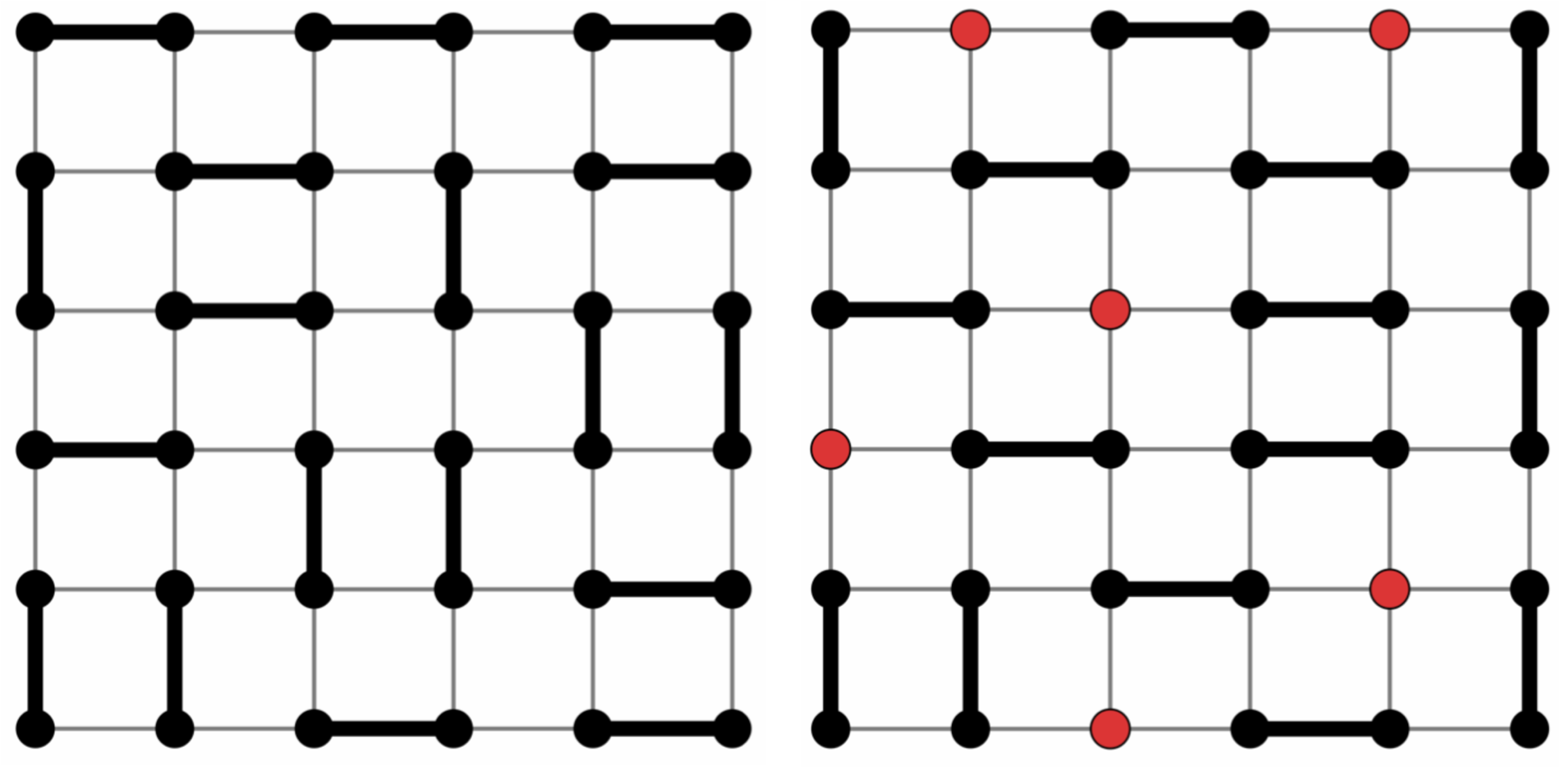
Figure 1: Dimer configurations in a $6\times 6$ square lattice [11]. (Left) Perfect matching without monomer. (Right) Dimers with monomers (red dots).

The term “domino” can have several meanings. Basically, a domino is a twofold object belonging to the polyomino family. It is encountered in statistical physics in the form of a “dimer” [8, 9] as a pure tiling problem or closely related to short–range interaction coupling in spin systems [10] (Fig. 1). It is also correlated with the alternating–sign matrices [12] and the square–ice model of statistical mechanics [13, 14]: namely, the six possible patterns for a vertex in a 4–regular digraph with two incoming arcs and two outgoing arcs. But the most amazing result is the existence of a circular area at the thermodynamic limit –the “Arctic Circle”– induced by random domino tilings in the Aztec diamond [15].

Our domino entity herein is quite different. Let $\mathcal{B}=\{e_{x},e_{y}\}=\{(1,0),(0,1)\}$ be the orthonormal basis in the $\mathbb{Z}\times\mathbb{Z}$ lattice and let

$$\mathcal{M}\,((x_{0},y_{0}\,))=\mathcal{M}_{r}\,((x_{0},y_{0}\,))=\{(x,y):|x-x_{0}|\leq r,|y-y_{0}|\leq r\}\ \ (r=1)$$

be the Moore neighborhood of range $r=1$ surrounding a given point $(x_{0},y_{0})$. Without loss of generality, let us choose the two neighboring points $\omega_{1}=(x_{1},y_{1}\,)$ and $\omega_{2}=(x_{2},y_{2})=\omega_{1}+e\ (e\in\mathcal{B})$ and the vector $\omega_{1}\omega_{2}$ anchored at $\omega_{1}$. A domino $(\omega_{1},\omega_{2})$ is the set of the 12 points

$$\mathcal{D}_{\omega_{1}\,\omega_{2}}=\mathcal{M}(\omega_{1}\,)\cup\mathcal{M}(\omega_{2}\,)=\mathcal{M}(\omega_{1}\,)\cup\mathcal{M}(\omega_{1}+e\,)$$

and where $\mathcal{K}_{\omega_{1}\,\omega_{2}}=\{\omega_{1},\omega_{2}\}$ is the kernel while the set of the 10 points

$$\mathcal{H}_{\omega_{1}\,\omega_{2}}=\mathcal{D}_{\omega_{1}\,\omega_{2}}-\mathcal{K}_{\omega_{1}\,\omega_{2}}$$

surrounding the kernel is the hull. Points in $\mathbb{Z}^{2}$ and cells in the cellular space are associated by duality as shown in Fig. 2.

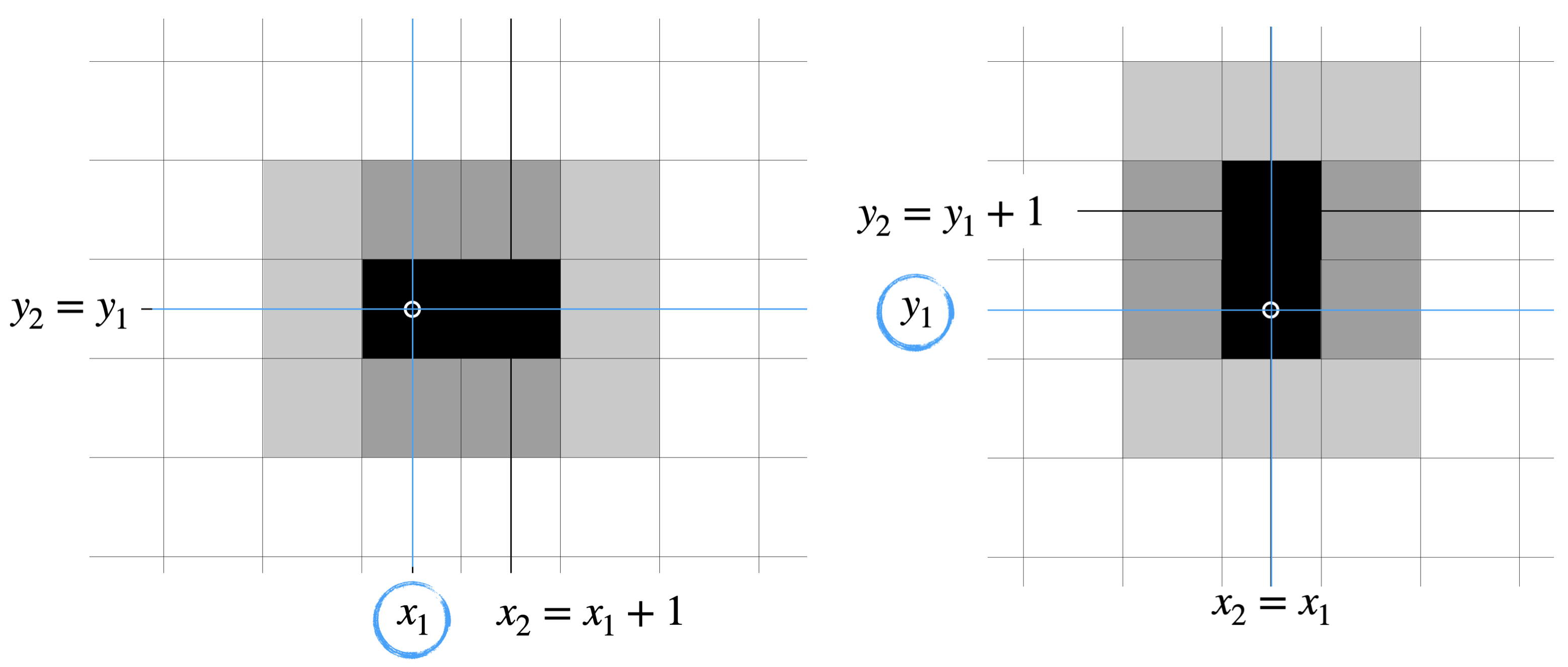
Figure 2: Horizontal and vertical dominos as the union of two Moore neighborhoods $\mathcal{M}(\omega_{1}\,)\cup\mathcal{M}(\omega_{2}\,)$ anchored at point $\omega_{1}$ in the $\mathbb{Z}^{2}$ lattice.

Horizontal and vertical dominos are such that $e=e_{x}$ and $e=e_{y}$ respectively.

Perhaps the best way to remove the troublesome homonymy from its namesake in statistical physics would be to rename our composite domino herein. A name like “$\{4,3\}$–do–deca–mino” (do– for kernel, deca– for hull) might then be more relevant.

A layout of dominos, whether maximum or minimum, is governed by the hull–kernel repulsive exclusion rule

$$\forall\omega_{1}\in\mathbb{Z}^{2}\ ;\ \forall\omega^{\prime}_{1}\in\mathbb{Z}^{2}\ :\ \mathcal{H}_{\omega^{\prime}_{1}\,\omega^{\prime}_{2}}\cap\mathcal{K}_{\omega_{1}\,\omega_{2}}=\varnothing$$

for any pair $(\mathcal{D}_{\omega_{1}\,\omega_{2}},\mathcal{D}_{\omega^{\prime}_{1}\,\omega^{\prime}_{2}}).$ This means, on the contrary, that the hulls of local neighbors are allowed to overlap. Each cell $\omega\in\mathbb{Z}^{2}$ is assigned a cover (or overlap) level $v_{\omega}\ (0\leq v_{\omega}\leq 4)$ which measures the number of dominos covering it. A lacunar void is an empty cell $\omega$ such that $v_{\omega}=0$. The hull–kernel exclusion implies $v_{\omega_{1}}=v_{\omega_{2}}=1$ for any $\mathcal{K}_{\omega_{1}\,\omega_{2}}.$ Figure 3 shows various scenarios of overlapping.

The kernel of a domino is allowed to evolve strictly within a given convex shape. It follows that the hull will necessarily exceed the envelope of the convex. In the simplest case, if we consider a square array of size $n\times n$ in which a population of dominos will evolve, then the relevant convex will be the square $\mathcal{S}_{n}$ of size $(n+2)\times(n+2).$

One of the best down–to–earth metaphor illustrating our domino entity is the arrangement of cars in a car–park. The kernel is the car itself while the hull is the free space left to open the doors, the tailgate or possibly the hood. Incidentally, the diamond might represent a complex idealized host shape – the parking lot – that could exist in old city centers or in steep regions. Similar physical distancing situations are found in structures such as a set of tables in a classroom or in any public space. Our problem of maximal arrangement of dominos fits into the broad subject of tiling and covering in two-dimensional spaces [16] and can be brought back to that of ellipsoid packing [17, 18].

2.2 Density Measurement

For a given domino $(\omega_{1},\omega_{2})$ we define the two following measures:

• the overlap index

  $$\nu_{\omega_{1},\omega_{2}}=\sum_{\mathcal{D}_{\omega_{1}\,\omega_{2}}}v_{\omega}=\sum_{\mathcal{K}_{\omega_{1}\,\omega_{2}}}v_{\omega}+\sum_{\mathcal{H}_{\omega_{1}\,\omega_{2}}}v_{\omega}=2+\sum_{\mathcal{H}_{\omega_{1}\,\omega_{2}}}v_{\omega}$$

  as the sum of all cover levels $v_{\omega}$ on $\omega\in\mathcal{D}_{\omega_{1}\,\omega_{2}}$ and

• the occupancy index

  $$\rho_{\omega_{1},\omega_{2}}=\sum_{\mathcal{D}_{\omega_{1}\,\omega_{2}}}\tau_{\omega}=\sum_{\mathcal{K}_{\omega_{1}\,\omega_{2}}}\tau_{\omega}+\sum_{\mathcal{H}_{\omega_{1}\,\omega_{2}}}\tau_{\omega}=2+\sum_{\mathcal{H}_{\omega_{1}\,\omega_{2}}}\tau_{\omega}$$

  where $\tau_{\omega}$ is the occupancy ratio (the inverse $1/v_{\omega}$ of the cover level) of cell $\omega\in\mathcal{D}_{\omega_{1}\,\omega_{2}}.$

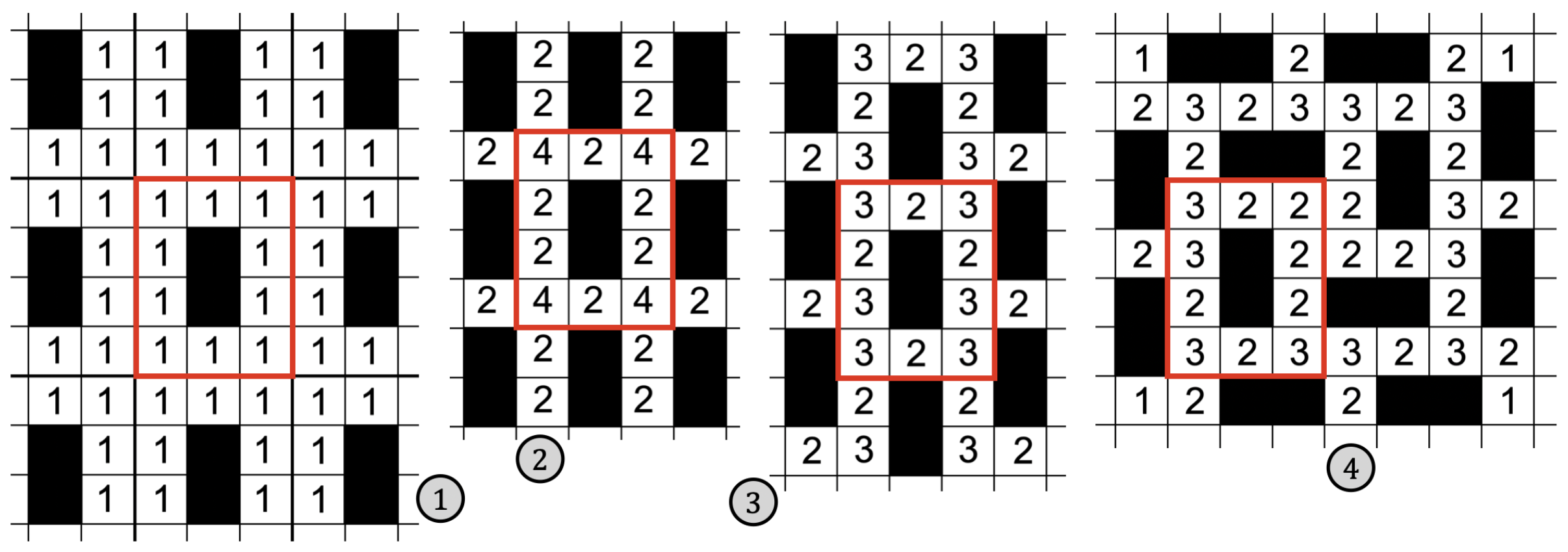
Figure 3: Four typical arrangements of dominos: (1) loosely coupled physical distancing configuration (2) tightly coupled orthotropic configuration (3) tightly coupled staggered configuration (4) tightly coupled isotropic configuration.

For example, the two measures above applied to the red domino in the four cases of Fig. 3 give:

1. $\nu_{\omega_{1},\omega_{2}}=2+10\times 1=12$  ;              $\rho_{\omega_{1},\omega_{2}}=2+10\times 1=12$

2. $\nu_{\omega_{1},\omega_{2}}=2+6\times 2+4\times 4=30$  ;     $\rho_{\omega_{1},\omega_{2}}=2+6\times 1/2+4\times 1/4=6$

3. $\nu_{\omega_{1},\omega_{2}}=2+4\times 2+6\times 3=28$  ;     $\rho_{\omega_{1},\omega_{2}}=2+4\times 1/2+6\times 1/3=6$

4. $\nu_{\omega_{1},\omega_{2}}=2+6\times 2+4\times 3=26$  ;       $\rho_{\omega_{1},\omega_{2}}=2+6\times 1/2+4\times 1/3=19/3$

In the first case, the overlap index is minimal while the occupancy index is maximal for a minimal layout. Depending of their objective function, the first and the second configurations are optimal, but an overall configuration is constrained by the boundary conditions. Second and third cases show better accuracy for the overlap index. Finally, the occupancy index provides a relationship between the number of dominos and the surface of the shape. Thus, if we reconsider the square $\mathcal{S}_{n}$ it follows that

$$\sum_{k=1}^{\xi_{n}}\rho\,(k)+\varpi_{n}\,=\ \mid\mathcal{S}_{n}\mid\ =(n+2)^{2}$$ (1)

where $\xi_{n}$ denotes the number of dominos for a given population in the square while $\rho\,(k)$ and $\varpi_{n}$ represent respectively the occupancy index of domino $k$ and the number of lacunar voids. Here $k$ defines an arbitrary numbering of the population of dominos. This relation holds whatever the population of dominos (either minimal or maximal, or neither minimal nor maximal).

2.3 Geometry of the Diamond

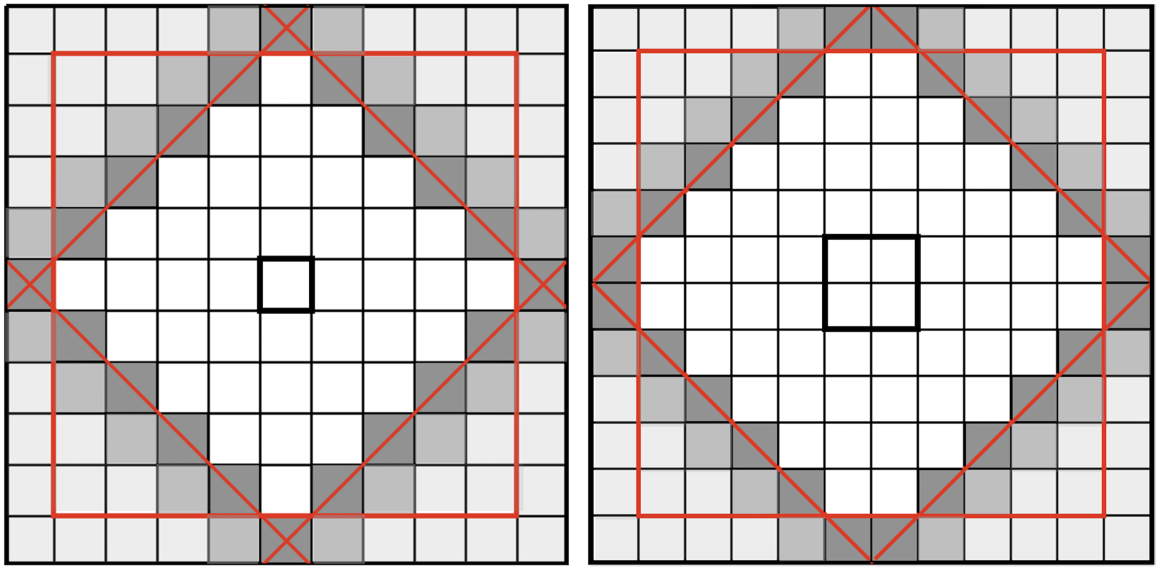
Figure 4: The (cellular) diamond $\mathcal{D}_{n}$ as a $\pi/4$–rotated (cellular) square.
– $n$ odd (left): $\mathcal{D}_{9}$ as a von Neumann neighborhood of range $r=5$ with $2r=n+1$ and $\mid\mathcal{D}_{n}\mid\ =n_{r}=61.$ For the white diamond $\mid\mathcal{D}_{n-2}\mid\ =n_{r-1}=41$ and for the full domain $\mid\mathcal{S}_{n}\cap\mathcal{D}_{n+2}\mid\,=n_{r+1}-4=81.$
– $n$ even (right): $\mathcal{D}_{10}$ as an Aztec diamond of range $r=6$ with $2r=n+2$ and $\mid\mathcal{D}_{n}\mid\ =n_{r}^{(a)}=84.$ For the white diamond $\mid\mathcal{D}_{n-2}\mid\ =n_{r-1}^{(a)}=60$ and for the full domain $\mid\mathcal{S}_{n}\cap\mathcal{D}_{n+2}\mid\,=n_{r+1}^{(a)}-8=104.$

The (cellular) diamond $\mathcal{D}_{n}$ is defined herein as a $\pi$/4–rotated square inscribed in a square array $\mathcal{S}_{n}$ of $(n+2)\times(n+2)$ cells including a border with perimeter $4n+4$ enclosing a $n\times n$ square (see $\mathcal{D}_{9}$ and $\mathcal{D}_{10}$ in Fig. 4).

The kernel of a domino is allowed to evolve within the white convex shape $\mathcal{D}_{n-2}.$ It follows that the hull will be able to occupy the domain defined by the tipless diamond $\mathcal{S}_{n}\cap\mathcal{D}_{n+2}$ where the four tips of $\mathcal{D}_{n+2}$ (1–cell tip for $n$ odd, 2–cell tip for $n$ even) lying outside $\mathcal{S}_{n}$ are truncated.

• $n$ odd : $\mathcal{D}_{n}$ has two perpendicular diagonals of length $n+2$ and a center cell. It is the von Neumann neighborhood of range $r$ at point $(0,0)$ (the center of $\mathcal{D}_{n}$) and such that $2r=n+1.$ $\mathcal{D}_{n}$ is then the set of cells whose centers $(x,y)$ are such that $\{(x,y):|\,x\,|+|\,y\ |\leq r\,\}\ (r\in\mathbb{N})$ and so that both $x$ and $y$ are integers. The cardinality of $\mathcal{D}_{n}$ is the centered square number $n_{r}=2r^{2}+2r+1$ whence

  $$|\mathcal{D}_{n}|=(n^{2}+4\,n+5)/2$$ (2)

  thus $\mid\mathcal{D}_{n-2}\mid\ =2r^{2}-2r+1$ and $\mid\mathcal{S}_{n}\cap\mathcal{D}_{n+2}\mid\,=2r^{2}+6r+1\,.$

• $n$ even : $\mathcal{D}_{n}$ has two perpendicular double diagonals of length $n+2$ and a 4–cell center centered at point $(0,0)$. It is the Aztec diamond $\mathcal{AD}_{r}$ of range $r$ and such that $2r=n+2.$ $\mathcal{D}_{n}$ is then the set of cells whose centers $(x,y)$ are such that $\{(x,y):|\,x\,|+|\,y\ |\leq r\,\}\ (r\in\mathbb{N}^{\ast})$ and so that both $x$ and $y$ are half–integers. It is the concatenation of 4 contiguous staircase quadrants, each containing ($1+2+\ldots+r$) cells, then the cardinality of $\mathcal{D}_{n}$ is $|\mathcal{AD}_{r}|=n_{r}^{(a)}=2r\,(r+1)$ whence

  $$|\mathcal{D}_{n}|=(n^{2}+6\,n+8)/2$$ (3)

  thus $\mid\mathcal{D}_{n-2}\mid\ =2r\,(r-1)$ and $\mid\mathcal{S}_{n}\cap\mathcal{D}_{n+2}\mid\,=2r^{2}+6r-4\,.$

The cardinality of the diamond satisfies the following relation

$$|\mathcal{D}_{n}|-|\mathcal{D}_{n-1}|=\left\{\begin{array}[]{ll}1&\mbox{ if }n\mbox{ odd }\\ 2n+3&\mbox{ if }n\mbox{ even }\end{array}\right.$$ (4)

and it suffices to notice that $n-1$ is even when $n$ is odd –and vice versa– then to adjust the cardinality of $\mathcal{D}_{n-1}$ accordingly.

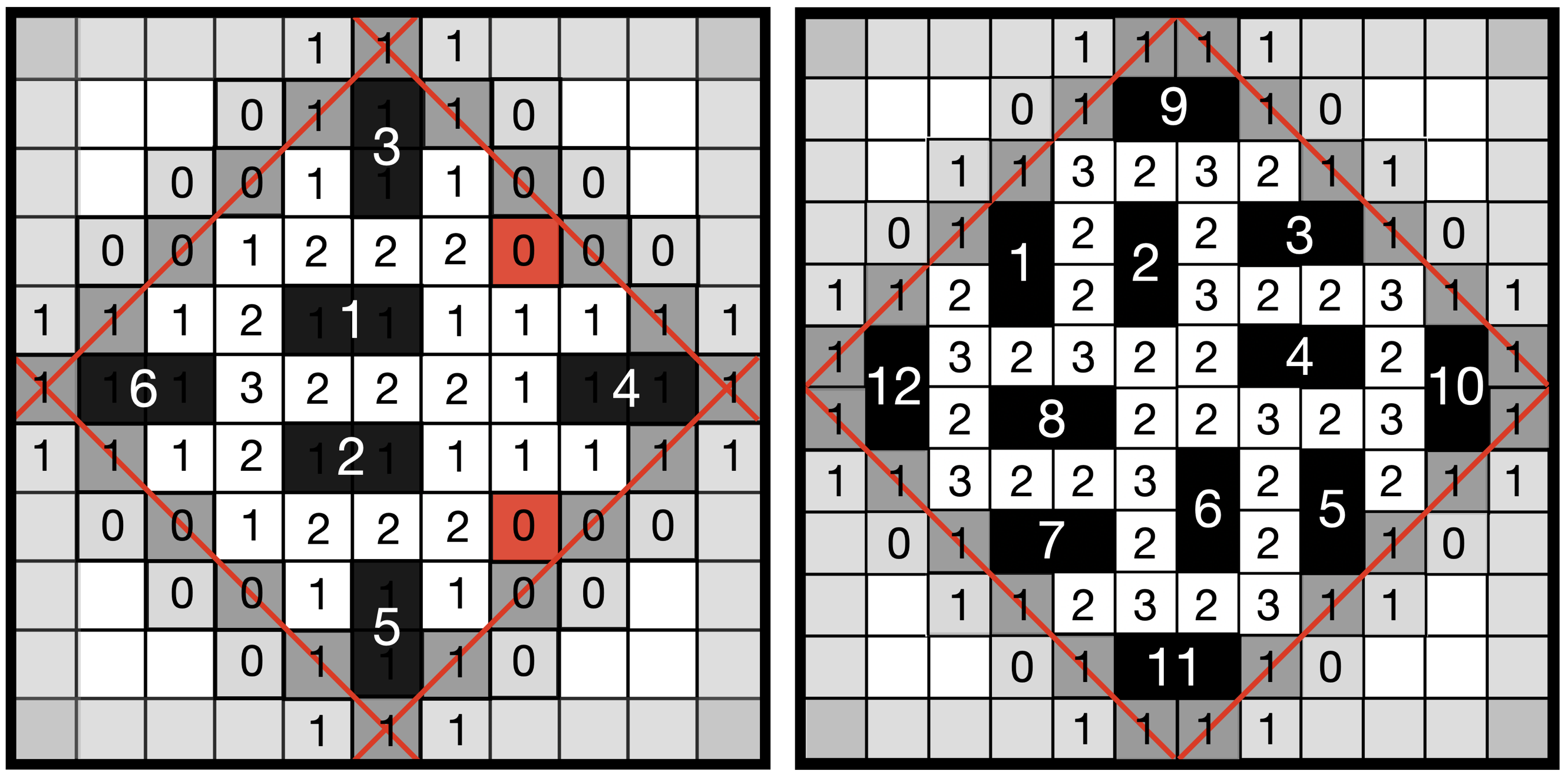
Figure 5: Connecting density and surface for a given population of dominos in $\mathcal{D}_{9}$ and $\mathcal{D}_{10}$. Dominos are numbered in the range $k\in[1,\psi_{n}].$

Finally, it is useful to revisit the relationship in (1) connecting a number of dominos and the surface of a shape from the occupancy index. Applied to the diamond it will follow that

$$\sum_{k=1}^{\psi_{n}}\rho\,(k)+\varpi_{n}\,=\ \mid\mathcal{S}_{n}\cap\mathcal{D}_{n+2}\mid$$ (5)

where $\psi_{n}$ denotes the number of dominos for a given population in $\mathcal{D}_{n}$ while $\rho\,(k)$ and $\varpi_{n}$ represent respectively the occupancy index of domino $k$ and the number of lacunar voids. As displayed in Fig. 5

• in $\mathcal{D}_{9}$ : $\rho(1)=\rho(2)=47/6;\ \rho(3)=\rho(5)=63/6;\ \rho(4)=72/6;\ \rho(6)=62/6\\$

  $$\Rightarrow\sum_{k=1}^{6}\rho\,(k)=59\ ;\hskip 11.38109pt\varpi_{9}=2+4\,(2+3)=22\hskip 5.69054pt\mbox{ and }\mid\mathcal{S}_{9}\cap\mathcal{D}_{11}\mid\,=81$$

• in $\mathcal{D}_{10}$ : note the rotational symmetry for $k\in(1,3,5,7)$ and $k\in(2,4,6,8)$ and $k\in(9,10,11,12).$ Now $\rho(1)=24/3;\ \rho(2)=19/3;\ \rho(9)=29/3\\$

  $$\Rightarrow\sum_{k=1}^{12}\rho\,(k)=96\ ;\hskip 11.38109pt\varpi_{10}=4\times 2=8\hskip 5.69054pt\mbox{ and }\mid\mathcal{S}_{10}\cap\mathcal{D}_{12}\mid\,=104$$

and it will be observed in the sequel that among these two configurations, that of $\mathcal{D}_{10}$ is maximal while that of $\mathcal{D}_{9}$ is not.

2.4 The Construction Rule

Unlike the dimer problem in statistical physics, which lists the number of all possible configurations for a given size shape, the more modest goal of this paper is to provide an exact value for the maximum number of dominos that can be contained in the diamond, or at least to provide lower and upper bounds.

We give here a heuristic approach. The analysis proceeds either according to an inductive formulation or according to a direct formulation. The inductive formulation makes it possible to underline certain recurrence relations. It will be observed that the geometry of the domino will involve a distribution of the patterns divided into six classes according to the size $n$ of the sample. In order to simplify the description, it will therefore be possible to proceed by “expansion” within the same class. The theoretical measures will split into six tables in the appendix, with a sample of up to $n=200$.

Our domino arrangement follows a recursive scheme, organized around a square central “core” and four N–S–E–W triangular “wedges”, symmetric by rotation as shown in Fig. 6. The case $n$ even is more intricate and the wedge must be divided into two subregions.

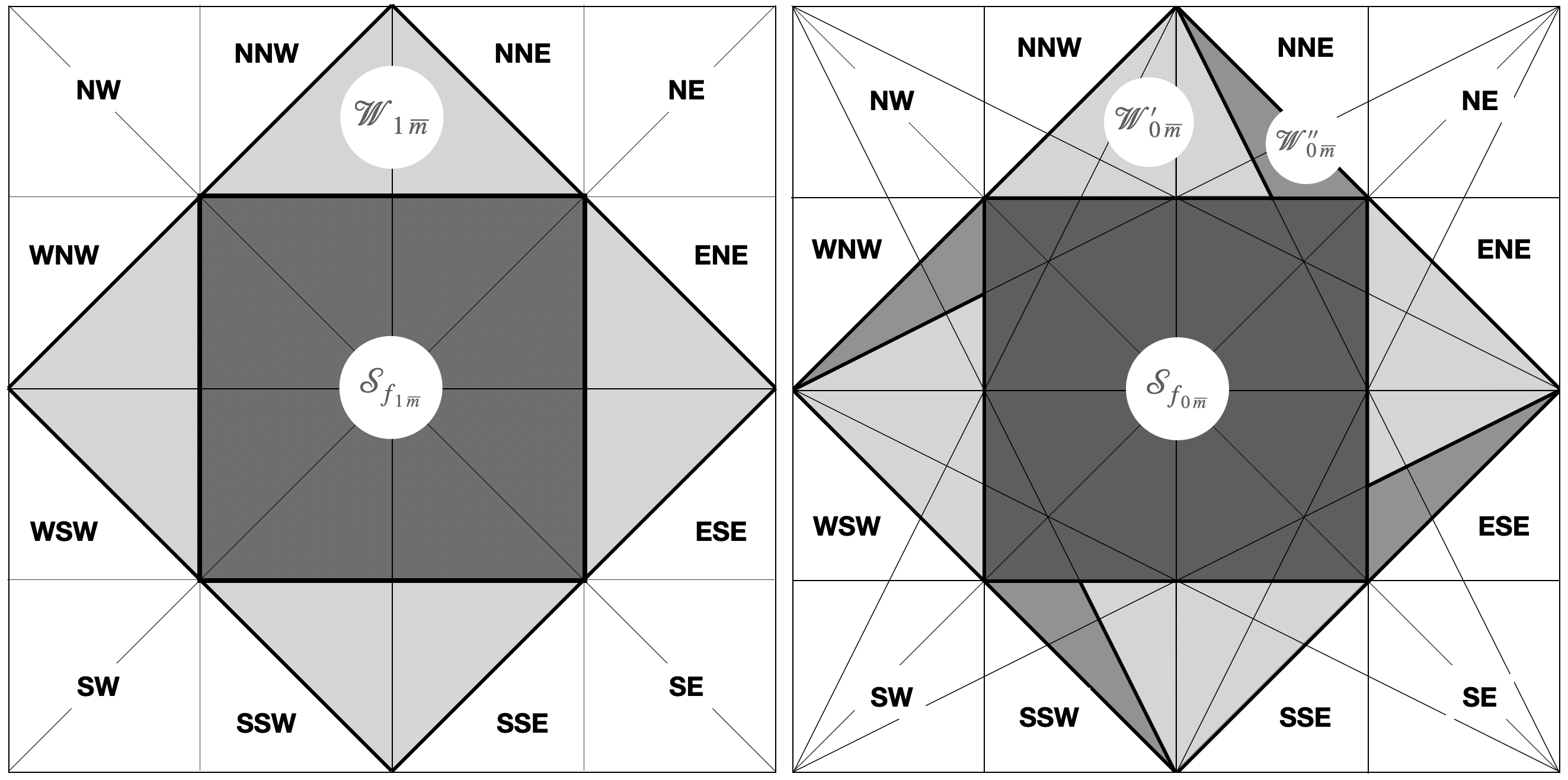
Figure 6: The (cellular) diamond $\mathcal{D}_{n}$ divided into regions.
– $n$ odd (left): a square central core $\mathcal{S}_{f_{1\overline{m}}}$ of size $f_{1\overline{m}}\approx m$ and four symmetric wedges $\mathcal{W}_{\,1\,\overline{m}}$ in N–S–E–W directions.
– $n$ even (right): a square central core $\mathcal{S}_{f_{0\overline{m}}}$ of size $f_{0\overline{m}}\approx m$ and four symmetric wedges $\mathcal{W}_{\,0\,\overline{m}}$ in N–S–E–W directions. Region $\mathcal{W}_{\,0\,\overline{m}}$ splits into two subregions: $\mathcal{W}^{\prime}_{\,0\,\overline{m}}$ and $\mathcal{W}^{\prime\prime}_{\,0\,\overline{m}}.$

The capacity, in number of dominos, of the square shape and the configurations for different sizes of the core are evaluated in Sect. 3. Setting $m=\lfloor n/2\rfloor$ and $p=\lfloor m/3\rfloor$ this hierarchy of configurations can then be divided into six equivalence classes. In the sequel, any function, say $\mathcal{F},$ is indexed by the pair ${\,\overline{n}\,\overline{m}}$ – often denoted as $({\overline{n\,m}})$ or $n\,m$ for short – where $\overline{n}$ stands for the class of $n$ modulo 2 (its parity) and where $\overline{m}$ stands for the class of $m$ modulo 3. Whence the six families of configurations, namely $(00),(01),(02)$ for $n$ even and $(10),(11),(12)$ for n odd. The first configurations for small values of $n$ are displayed in Figs. 8–8.

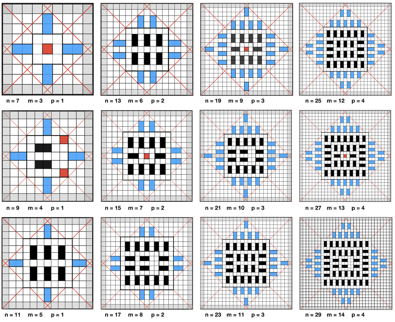
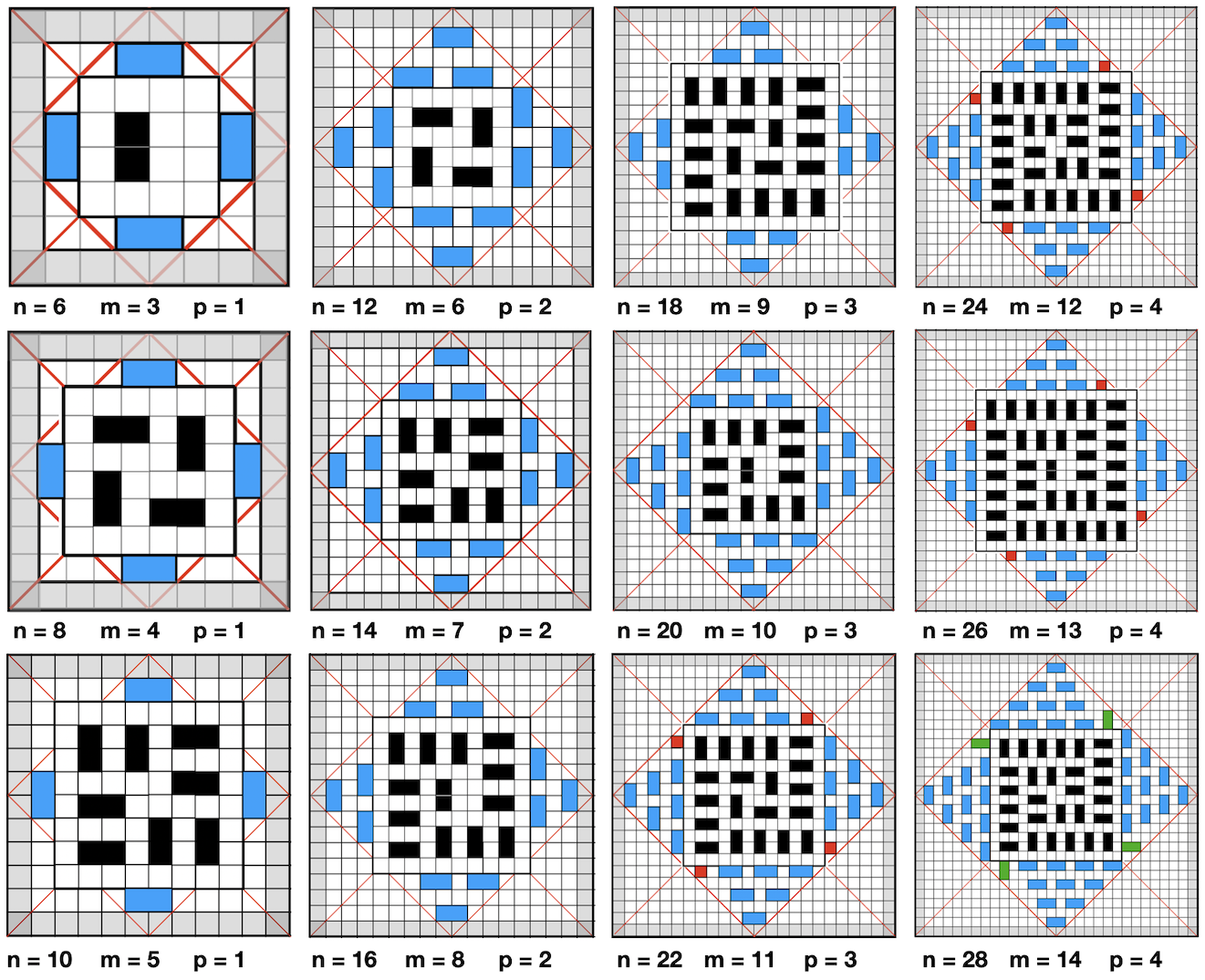
Figure 7: – $n$ odd. The first configurations with small values of $p\hskip 2.84526pt(p>0)$. From top to bottom: Class ${10}$, Class ${11}$, Class ${12}$. Some lacunar voids are integral part of the core.

Figure 8: – $n$ even. The first configurations with small values of $p\hskip 2.84526pt(p>0)$. From top to bottom: Class ${00}$, Class ${01}$, Class ${02}$. Some lacunar voids emerge as isolated cells from $n>20$.

In this NP problem of domino arrangement, this arbitrary choice of construction around a central square whose side length $f_{\overline{n}\,\overline{m}}\approx m$ is determined and where several solutions can coexist, the exact definition of this function must be considered as the axiom, from which the placement of dominos follows a logical approach.

Besides, the case $n$ even argues for a “horizontal” arrangement of the dominos with respect to the North wedge (parallel to the adjacent North side of the core) while the case $n$ odd argues for a “vertical” arrangement (perpendicular to the adjacent core’s side). In addition, a rotational symmetry of the wedges is required. We could dare the analogy, in a rather relative measure, with the observation of the authors except that theirs results from a physical phenomenon whereas ours results only from a rule of construction.

Finally, the placement of the dominos is organized from the left part of the (North) wedge, even if it leads to the completion of the inner right border with lacunar voids. Based on these criteria, our theoretical arrangement of dominos is unique. The analysis is developed in Sect. 4–5. The penultimate column of the last six tables in the appendix (Tabs. 8–13) lists the value $\psi_{n}$ representing the lower bound reached at the end of this construction.

2.5 Injection of Disorder

Our theoretical arrangement is almost optimal, not totally optimal. For example, it would be easy to observe in Fig. 8 and in more detail in Fig. 5 that the diamond could accept at least $7$ dominos for $n=9$. Nevertheless, by relaxing the constraint, it is possible to inject disorder into the model in order to increase its population density. The counting of lacunar voids – emerging in Fig. 8 from $n>20$ in a systematic way – will also be considered: in a disordered system, lacunar voids could indeed join together and thus form a new domino. In Sect. 6, different scenarios of injection are examined on a case–by–case basis. The aim is to achieve tight upper bounds whenever possible. The last column of Tabs. 8–13 lists the value $\overline{\psi}_{n}$ representing the upper bound reached at the end of this injection. In some cases, the lower and upper bounds coincide, so $\overline{\psi}_{n}=\psi_{n}$ and $\psi_{n}$ becomes the exact number of dominos for a maximum configuration.

3 Dominos in the Square

Given a square array $\mathcal{S}_{n}$ of $(n+2)\times(n+2)$ cells including a border with perimeter $4n+4$ enclosing the $n\times n$ field $\mathcal{S}_{n-2}$ of order $n^{2}$.

The chosen arrangement is organized in concentric crowns surrounding a basic motif of minimal size. By construction, induced by the morphology of the domino, the successive crowns will be of thickness 3. It follows that the square shapes will be divided into six equivalence classes $\dot{n}\,\dot{m}$ –or shortly $(\dot{nm})$ –where $\dot{n}$ stands for the class of $n$ modulo 2 (its parity) while $\dot{m}$ stands for the class of $m$ modulo 3. Whence the six families of configurations, namely $(\dot{10}),(\dot{11}),(\dot{12})$ for $n$ odd and $(\dot{00}),(\dot{01}),(\dot{02})$ for $n$ even. The first configurations for small values of $n$ are displayed in Fig. 9.

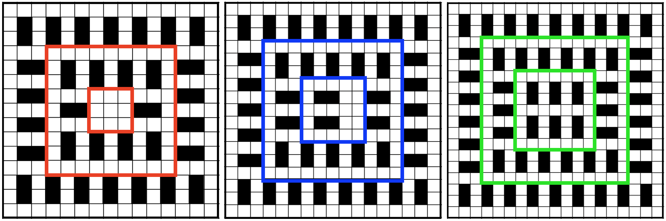
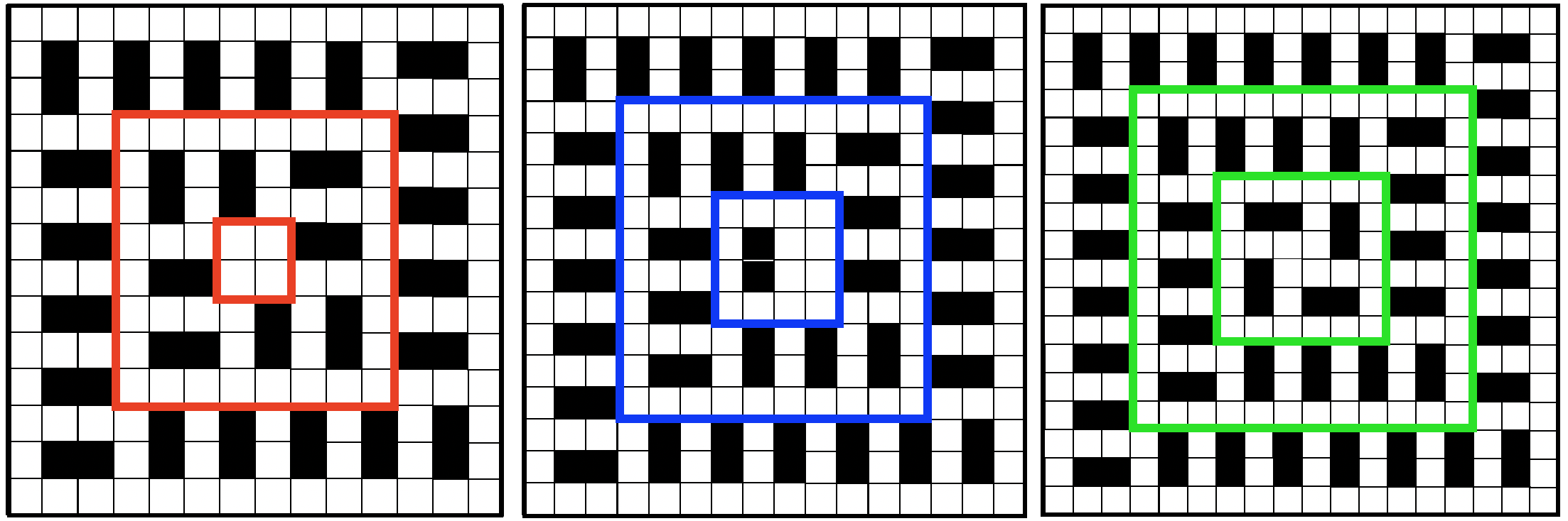
Figure 9: Dominos in the square $\mathcal{S}_{n}$.
$(\uparrow)$ The first configurations for $n$ odd, from left to right:
Class $(\dot{10})$: $(\mathcal{S}_{1},\mathcal{S}_{7},\mathcal{S}_{13}),$ Class $(\dot{11})$: $(\mathcal{S}_{3},\mathcal{S}_{9},\mathcal{S}_{15}),$ Class $(\dot{12})$: $(\mathcal{S}_{5},\mathcal{S}_{11},\mathcal{S}_{17}).$
$(\downarrow)$ The first configurations for $n$ even, from left to right:
Class $(\dot{00})$: $(\mathcal{S}_{0},\mathcal{S}_{6},\mathcal{S}_{12}),$ Class $(\dot{01})$: $(\mathcal{S}_{2},\mathcal{S}_{8},\mathcal{S}_{14}),$ Class $(\dot{02})$: $(\mathcal{S}_{4},\mathcal{S}_{10},\mathcal{S}_{16}).$

The maximal domino number $\xi_{n}(\mathcal{S}_{n})$ covering $\mathcal{S}_{n}$ is given by the inductive formula

$$n\hskip 5.69054pt\mbox{odd:}\hskip 14.22636pt\xi_{1}=0,\,\xi_{3}=2,\,\xi_{5}=6\hskip 14.22636pt\mbox{and}\hskip 14.22636pt\xi_{n}=\xi_{n-6}+2(n-2)\vspace{-2mm}$$ (6)

$$n\hskip 5.69054pt\mbox{even:}\hskip 11.38109pt\xi_{0}=0,\,\xi_{2}=1,\,\xi_{4}=4\hskip 14.22636pt\mbox{and}\hskip 14.22636pt\xi_{n}=\xi_{n-6}+2(n-2)\vspace{-1mm}$$ (7)

for $n\geq 6$ and where $2(n-2)$ denotes the number of dominos in the crown surrounding the inner subgrid $\mathcal{S}_{n-6}.$ A proof is straightforward: the crown $\widehat{\mathcal{S}}_{n}$ of size $\mid\widehat{\mathcal{S}}_{n}\mid=4((n+1)+(n-1)+(n-3))=12(n-1)$ yields a domino area (excluding border) with size $\mid\widehat{\mathcal{S}}_{n}\mid-(4n+4)=4(2n-4)$ whence the number $(2n-4)$ of black–white tetraminos.

The exact expressions of $\xi_{n}$ depend on the class of $\mathcal{S}_{n}$ and are given hereafter.

3.1 $n$ odd — $\xi_{n}$

Depending on the class of $m\bmod 3,$ it follows from (6) that in

• $\mbox{ {Class} $(\dot{10})$ : }m\equiv 0\hskip 2.84526pt\Rightarrow\hskip 2.84526ptn=6\,p+1\hskip 5.69054pt\mbox{and then}$

  $$\xi_{n}=\xi_{1}+2\sum_{k=1}^{p}(6\,k-1)=2p\,(3p+2)=\frac{(n-1)(n+3)}{6}\vspace{-3mm}$$ (8)

• $\mbox{ {Class} $(\dot{11})$ : }m\equiv 1\hskip 2.84526pt\Rightarrow\hskip 2.84526ptn=6\,p+3\hskip 5.69054pt\mbox{and then}$

  $$\xi_{n}=\xi_{3}+2\sum_{k=1}^{p}(6\,k+1)=2+2p\,(3p+4)=\frac{(n-1)(n+3)}{6}\vspace{-3mm}$$ (9)

• $\mbox{ {Class} $(\dot{12})$ : }m\equiv 2\hskip 2.84526pt\Rightarrow\hskip 2.84526ptn=6\,p+5\hskip 5.69054pt\mbox{and then}$

  $$\xi_{n}=\xi_{5}+2\sum_{k=1}^{p}(6\,k+3)=6+2p\,(3p+6)=\frac{(n+1)^{2}}{6}\vspace{-3mm}$$ (10)

3.2 $n$ even — $\xi_{n}$

Depending on the class of $m\bmod 3,$ it follows from (7) that in

• $\mbox{ {Class} $(\dot{00})$ : }m\equiv 0\hskip 2.84526pt\Rightarrow\hskip 2.84526ptn=6\,p\hskip 5.69054pt\mbox{and then}$

  $$\xi_{n}=\xi_{0}+2\sum_{k=1}^{p}(6\,k-2)=2p\,(3p+1)=\frac{n\,(n+2)}{6}\vspace{-3mm}$$ (11)

• $\mbox{ {Class} $(\dot{01})$ : }m\equiv 1\hskip 2.84526pt\Rightarrow\hskip 2.84526ptn=6\,p+2\hskip 5.69054pt\mbox{and then}$

  $$\xi_{n}=\xi_{2}+2\sum_{k=1}^{p}6\,k=1+2p\,(3p+3)=\frac{n(n+2)-2}{6}\vspace{-3mm}$$ (12)

• $\mbox{ {Class} $(\dot{02})$ : }m\equiv 2\hskip 2.84526pt\Rightarrow\hskip 2.84526ptn=6\,p+4\hskip 5.69054pt\mbox{and then}$

  $$\xi_{n}=\xi_{4}+2\sum_{k=1}^{p}(6\,k+2)=4+2p\,(3p+5)=\frac{n(n+2)}{6}\vspace{-2mm}$$ (13)

The 100 first values of $\xi_{n}$ are displayed in Tabs. 6–7 in the appendix.

4 Dominos in the Diamond — $n$ odd

The following constructions for $\overline{1\,m}$ classes (often denoted as “$1m$” from now on) are valid only when the core–wedge structure actually appears from Fig. 8, that is, for $p\geq 1$. When growth formulas are used for the expansion of different regions, the strict condition $p>1$ is required. In the sequel, these conditions will be assumed everywhere, unless mentioned otherwise. The first configurations with $p=0$ are shown in Fig. 10.

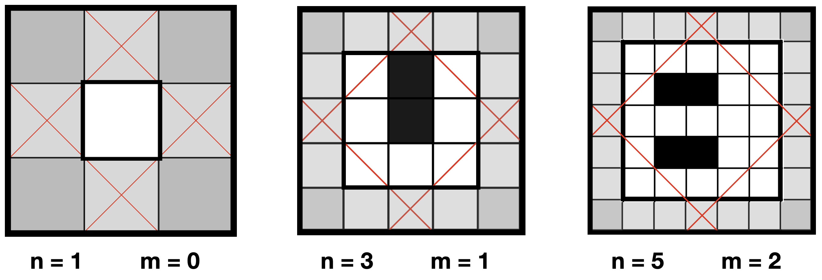
Figure 10: – $n$ odd. The first configurations with $p=0$. From left to right: Class ${10}$ ($\psi_{1}=0$), Class ${11}$ ($\psi_{3}=1$), Class ${12}$ ($\psi_{5}=2$).

The case $n$ odd argues for a “vertical” layout of the dominos (perpendicular to the adjacent core’s side). Referring back to Fig. 6 (left) the exact size $f_{1m}\approx m$ of the core will be adjusted so that the configuration of the wedges is entirely fixed by the $p$ parameter. Let $f_{1m}^{+}(m)=f_{1m}(m)+2$ be the extended length of the side of $\mathcal{S}_{f_{1m}(m)}$ including borders, and let $h_{1m}$ such that

$$f_{1m}^{+}(m)=n-2\cdot h_{1m}(p)\hskip 28.45274pt(n=2m+1)$$

where $h_{1m}$ is the height of the vertical median column of Region $\mathcal{W}_{1m}.$ By observing that this wedge is an isosceles right triangle, we fix its height so that

$$2\cdot h_{1m}(p)=3p+\mu_{p}\hskip 5.69054pt\mbox{ with }\hskip 5.69054pt\mu_{p}=\left\{\begin{array}[]{ll}0&\mbox{ for }p\mbox{ even }\\ 1&\mbox{ for }p\mbox{ odd }\end{array}\right.$$ (14)

and it follows that

$$f_{1m}^{+}(m)=\left\{\begin{array}[]{ll}(6p+1)-(3p+\mu_{p})=3p+1-\mu_{p}&\mbox{ in {Class} $10$ }\\ (6p+3)-(3p+\mu_{p})=3p+3-\mu_{p}&\mbox{ in {Class} $11$ }\\ (6p+5)-(3p+\mu_{p})=3p+5-\mu_{p}&\mbox{ in {Class} $12$ }\end{array}\right.$$

whence finally the strict length of the side in the square core

$$f_{1m}(m)=f_{1m}^{+}(m)-2=\left\{\begin{array}[]{ll}m-1-\mu_{p}&\mbox{ in {Class} $10$ }\\ m-\mu_{p}&\mbox{ in {Class} $11$ }\\ m+1-\mu_{p}&\mbox{ in {Class} $12$ }\end{array}\right.$$ (15)

now expressed in terms of $m$. Or, by using a general notation unifying the three classes

$$f_{1m}(m)=(m-1+m\bmod 3)-\mu_{p}$$ (16)

for any $m>0$. Moreover, with $\mu_{p-1}=1-\mu_{p}$ we get

$$f_{1m}(m)-f_{1m}(m-3)=3-\mu_{p}+\mu_{p-1}=4-2\,\mu_{p}=\left\{\begin{array}[]{ll}+4&\mbox{ for }p\mbox{ even }\\ +2&\mbox{ for }p\mbox{ odd }\end{array}\right.$$ (17)

giving the elongation of the side of the square core within a $p-1\rightarrow p$ expansion.

4.1 Class $10$ — $n$ odd   &   $m\equiv 0\pmod{3}$

The basic parameters of Class $10$ verify:

$$p\,\in\,\mathbb{N}\,;\hskip 8.53581ptm\,=3\,p\,;\hskip 8.53581ptn\,=2\,m\,+1\,;$$

4.1.1 Capacity and expansion rate of the square core $\mathcal{S}_{f_{10}}$

From (15–16) $f_{10}(m)=m-1-\mu_{p}$ and we get the following two cases

• $\mu_{p}=0\Rightarrow f_{10}(m)=m-1$ and $(m-1)/2\in\dot{2}\hskip 2.84526pt\mbox{in}\hskip 2.84526pt\mathbb{Z}/3\,\mathbb{Z}$ then $\xi_{m-1}$ follows from (10) whence

  $$\xi_{m-1}=\frac{m^{2}}{6}$$ (18)

• $\mu_{p}=1\Rightarrow f_{10}(m)=m-2$ and $(m-2)/2\in\dot{0}\hskip 2.84526pt\mbox{in}\hskip 2.84526pt\mathbb{Z}/3\,\mathbb{Z}$ then $\xi_{m-2}$ follows from (8) whence

  $$\xi_{m-2}=\frac{(m-3)(m+1)}{6}$$ (19)

giving the capacity of the square core. In the same way, from (17) we get the following two cases

• $\mu_{p}=0\Rightarrow f_{10}(m-3)=f_{10}(m)-4=m-5$ and $(m-5)/2\in\dot{0}$ then $\xi_{m-5}$ follows from (8) whence

  $$\xi_{m-1}-\xi_{m-5}=\frac{m^{2}}{6}-\frac{(m-6)(m-2)}{6}=\frac{4\,m-6}{3}=4\,p-2$$ (20)

• $\mu_{p}=1\Rightarrow f_{10}(m-3)=f_{10}(m)-2=m-4$ and $(m-4)/2\in\dot{2}$ then $\xi_{m-4}$ follows from (10) whence

  $$\xi_{m-2}-\xi_{m-4}=\frac{(m-3)(m+1)}{6}-\frac{(m-3)^{2}}{6}=\frac{2\,m-6}{3}=2\,p-2$$ (21)

giving the expansion rate for the capacity in the square core.

4.1.2 Capacity and expansion rate of the wedge $\mathcal{W}_{10}$

Let $W_{10}(p)$ be the capacity of the wedge for any given $p$. From (14) comes

$$2\,(\,h_{10}(p)+\mu_{p})=3\,(\,p+\mu_{p})$$

and thus we get the capacity of the vertical median of Region $\mathcal{W}_{10}$

$$\overline{h}_{10}(p)=(h_{10}(p)+\mu_{p})/3=(p+\mu_{p})/2$$

in number of vertical dominos –namely, in number of horizontal rows of dominos. The baserow of $\mathcal{W}_{10}$ has the length

$$b_{10}(p)=2\cdot h_{10}(p)-1=3p+\mu_{p}-1\hskip 8.53581pt$$

always odd. This baserow can accommodate a binary string of the form $(01)^{*}0$ of length $b_{10}(p)$ with $h_{10}(p)$ zeros and thereby a baserow with capacity

$$\overline{b}_{10}(p)=(b_{10}(p)-1)/2=(3p+\mu_{p}-2)/2$$

in number of vertical dominos. Now $\overline{h}_{10}(1)=1\hskip 2.84526pt\mbox{;}\hskip 5.69054pt\overline{b}_{10}(1)=1$ and

$$\overline{h}_{10}(p)-\overline{h}_{10}(p-1)=\mu_{p}\hskip 5.69054pt\mbox{and}\hskip 5.69054pt\overline{b}_{10}(p)-\overline{b}_{10}(p-1)=1+\mu_{p}\hskip 8.53581pt$$

whence the two following cases:

• $\mu_{p}=0\Rightarrow$ The number of rows remains unchanged during expansion, and the capacity of the baserow is increased by 1, as well as, by extension, the capacity of the $p/2$ rows. Then $W_{10}(p)-W_{10}(p-1)=p/2.$

• $\mu_{p}=1\Rightarrow$ The capacity of the baserow is increased by 2, as well as, by extension, the capacity of the $(p-1)/2$ rows $(p>1)$.The capacity of the median is increased by 1, by adding a new row with a single domino at the top of the wedge. Then $W_{10}(p)-W_{10}(p-1)=2\,(p-1)/2+1=p.$

It follows that

$$W_{10}(0)=0\hskip 2.84526pt\mbox{;}\hskip 5.69054ptW_{10}(p)-W_{10}(p-1)=\frac{p\,(1+\mu_{p})}{2}$$ (22)

yields the $p-1\rightarrow p$ expansion of Region $\mathcal{W}_{10}.$ Nevertheless, since $\mu_{p}+\mu_{p-1}=1$ the following expansion

$$\overline{h}_{10}(p)-\overline{h}_{10}(p-2)=1\hskip 5.69054pt\mbox{and}\hskip 5.69054pt\overline{b}_{10}(p)-\overline{b}_{10}(p-2)=3$$

is relevant and does not depend on the parity of $p$. As a result, the vertical median can accommodate one additional baserow extended with three additional dominos within any $p-2\rightarrow p$ expansion. For clarity’s sake, we distinguish the two cases

• $\mu_{p}=0:W_{10}(2)=\overline{b}_{10}(2)=2$ ; $W_{10}(p)=W_{10}(p-2)+(3\,p-2)/2$ and after the appropriate change of variable $p=2k$

  $$W_{10}(p)=\sum_{k=1}^{p/2}(3\,k-1)=\frac{p\,(3\,p+2)}{8}$$

• $\mu_{p}=1:W_{10}(1)=\overline{b}_{10}(1)=1$ ; $W_{10}(p)=W_{10}(p-2)+(3\,p-1)/2$ and after the appropriate change of variable $p=2k-1$

  $$W_{10}(p)=\sum_{k=1}^{(p+1)/2}(3\,k-2)=\frac{(p+1)(3\,p+1)}{8}$$

and finally

$$W_{10}(p)=\frac{(p+\mu_{p})\,(3\,p+2-\mu_{p})}{8}$$ (23)

or even in the form

$$W_{10}(p)=\frac{\overline{h}_{10}(p)\cdot(\overline{b}_{10}(p)+(2-\mu_{p}))}{2}$$ (24)

in order to emphasize that $W_{10}$ grows with the area of Triangle $\mathcal{W}_{10}.$

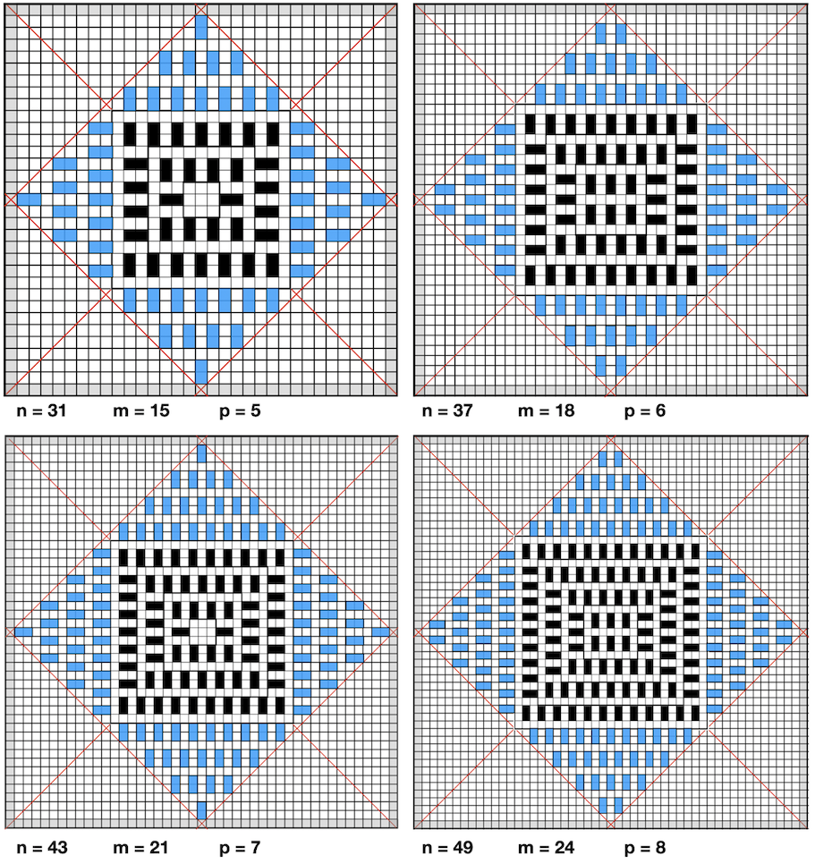
Figure 11: A 4–sequence of $\mathcal{D}_{n}$ expansion in Class $10$. The class of the square core $\mathcal{S}_{f_{10}(m)}$ alternates from $(\dot{10})$ to $(\dot{12})$ (refer to Fig. 9) whereas a new row is added in $\mathcal{W}_{10}$ for $p$ odd.

4.1.3 Capacity and expansion of $\mathcal{D}_{n}$ in Class $10$

The capacity $\psi_{n}$ of $\mathcal{D}_{n}$ in Class $10$ is simply given by

$$\psi_{n}=\xi_{f_{10}(m)}+4\,W_{10}(p)\vspace{-4mm}$$ (25)

and then

• $\mu_{p}=0\Rightarrow$ from (18) and from (23)

  $$\psi_{n}=\frac{m^{2}}{6}+\frac{p\,(3\,p+2)}{2}$$

• $\mu_{p}=1\Rightarrow$ from (19) and from (23)

  $$\psi_{n}=\frac{(m-3)(m+1)}{6}+\frac{(p+1)\,(3\,p+1)}{2}$$

and finally

$$\psi_{n}=p\,(3p+1)=\frac{(n-1)(n+1)}{12}$$ (26)

whatever the parity of $p$.

The expansion rate of $\psi_{n}$ can also be obtained stepwise: it follows from (20–21) and from (22) that is, with $p>0$

$$\psi_{n}-\psi_{n-6}=(\xi_{f_{10}(m)}-\xi_{f_{10}(m-3)})+4\,(W_{10}(p)-W_{10}(p-1))$$

$$=\mu_{p}\,(2\,p-2)+(1-\mu_{p})\,(4\,p-2)+2\,p\,(1+\mu_{p})=6\,p-2$$

now $n=2\,m+1$ and $m=3\,p$ then

$$\psi_{1}=0\ ;\hskip 5.69054pt\psi_{n}-\psi_{n-6}=n-3\,.$$ (27)

The values of $\psi_{n}$ in Class $10$ are displayed in Table 8. A 4–sequence of expansions is displayed in Fig. 11.

4.2 Class $11$ — $n$ odd   &   $m\equiv 1\pmod{3}$

The basic parameters of Class $11$ verify:

$$p\,\in\,\mathbb{N}\,;\hskip 8.53581ptm\,=3\,p+1\,;\hskip 8.53581ptn\,=2\,m\,+1\,;$$

4.2.1 Capacity and expansion rate of the square core $\mathcal{S}_{f_{11}}$

From (15–16) $f_{11}(m)=m-\mu_{p}$ and we get the following two cases

• $\mu_{p}=0\Rightarrow f_{11}(m)=m$ and $m/2\in\dot{0}\hskip 2.84526pt\mbox{in}\hskip 2.84526pt\mathbb{Z}/3\,\mathbb{Z}$ then $\xi_{m}$ follows from (8) whence

  $$\xi_{m}=\frac{(m-1)(m+3)}{6}$$ (28)

• $\mu_{p}=1\Rightarrow f_{11}(m)=m-1$ and $(m-1)/2\in\dot{1}\hskip 2.84526pt\mbox{in}\hskip 2.84526pt\mathbb{Z}/3\,\mathbb{Z}$ then $\xi_{m-2}$ follows from (9) whence

  $$\xi_{m-1}=\frac{(m-2)(m+2)}{6}$$ (29)

giving the capacity of the square core. In the same way, from (17) we get the following two cases

• $\mu_{p}=0\Rightarrow f_{11}(m-3)=f_{11}(m)-4=m-4$ and $(m-4)/2\in\dot{1}$ then $\xi_{m-4}$ follows from (9) whence

  $$\xi_{m}-\xi_{m-4}=\frac{(m-1)(m+3)}{6}-\frac{(m-5)(m-1)}{6}=\frac{4\,m-4}{3}=4\,p$$ (30)

• $\mu_{p}=1\Rightarrow f_{11}(m-3)=f_{11}(m)-2=m-3$ and $(m-3)/2\in\dot{0}$ then $\xi_{m-3}$ follows from (8) whence

  $$\xi_{m-1}-\xi_{m-3}=\frac{(m-2)(m+2)}{6}-\frac{m(m-4)}{6}=\frac{2\,m-3}{3}=2\,p$$ (31)

giving the expansion rate for the capacity in the square core.

Figure 12: A 4–sequence of $\mathcal{D}_{n}$ expansion in Class $11$. The class of the square core $\mathcal{S}_{f_{11}(m)}$ alternates from $(\dot{11})$ to $(\dot{10})$ (refer to Fig. 9) whereas a new row is added in $\mathcal{W}_{11}$ for $p$ odd.

4.2.2 Capacity and expansion of $\mathcal{D}_{n}$ in Class $11$

The capacity $\psi_{n}$ of $\mathcal{D}_{n}$ in Class $11$ is given by

$$\psi_{n}=\xi_{f_{11}(m)}+4\,W_{11}(p)$$ (32)

and with $W_{11}\equiv W_{10}$ we get

• $\mu_{p}=0\Rightarrow$ from (28) and from (23)

  $$\psi_{n}=\frac{(m-1)(m+3)}{6}+\frac{p\,(3\,p+2)}{2}$$

• $\mu_{p}=1\Rightarrow$ from (29) and from (23)

  $$\psi_{n}=\frac{(m-2)(m+2)}{6}+\frac{(p+1)\,(3\,p+1)}{2}$$

and finally

$$\psi_{n}=3p\,(p+1)=\frac{(n-3)(n+3)}{12}$$ (33)

whatever the parity of $p>0$.

The expansion rate of $\psi_{n}$ can also be obtained stepwise: it follows from (30–31) and from (22) that is, with $p>0$

$$\psi_{n}-\psi_{n-6}=(\xi_{f_{11}(m)}-\xi_{f_{11}(m-3)})+4\,(W_{11}(p)-W_{11}(p-1))$$

$$=2\,p\cdot\mu_{p}\,+4\,p\,(1-\mu_{p})\,+2\,p\,(1+\mu_{p})=6\,p$$

now $n=2\,m+1$ and $m=3\,p+1$ then

$$\psi_{1}=1\ ;\hskip 5.69054pt\psi_{n}-\psi_{n-6}=n-3\,.$$ (34)

The values of $\psi_{n}$ in Class $11$ are displayed in Table 9. A 4–sequence of expansions is displayed in Fig. 12.

4.3 Class $12$ — $n$ odd   &   $m\equiv 2\pmod{3}$

The basic parameters of Class $12$ verify:

$$p\,\in\,\mathbb{N}\,;\hskip 8.53581ptm\,=3\,p+2\,;\hskip 8.53581ptn\,=2\,m\,+1\,;$$

4.3.1 Capacity and expansion rate of the square core $\mathcal{S}_{f_{12}}$

From (15–16) $f_{12}(m)=m+1-\mu_{p}$ and we get the following two cases

• $\mu_{p}=0\Rightarrow f_{12}(m)=m+1$ and $(m+1)/2\in\dot{1}\hskip 2.84526pt\mbox{in}\hskip 2.84526pt\mathbb{Z}/3\,\mathbb{Z}$ then $\xi_{m+1}$ follows from (9) whence

  $$\xi_{m+1}=\frac{m(m+4)}{6}$$ (35)

• $\mu_{p}=1\Rightarrow f_{12}(m)=m$ and $m/2\in\dot{2}\hskip 2.84526pt\mbox{in}\hskip 2.84526pt\mathbb{Z}/3\,\mathbb{Z}$ then $\xi_{m}$ follows from (10) whence

  $$\xi_{m}=\frac{(m+1)^{2}}{6}$$ (36)

giving the capacity of the square core. In the same way, from (17) we get the following two cases

• $\mu_{p}=0\Rightarrow f_{12}(m-3)=f_{12}(m)-4=m-3$ and $(m-3)/2\in\dot{2}$ then $\xi_{m-3}$ follows from (10) whence

  $$\xi_{m+1}-\xi_{m-3}=\frac{m(m+4)}{6}-\frac{(m-2)^{2}}{6}=\frac{4\,m-2}{3}=4\,p+2$$ (37)

• $\mu_{p}=1\Rightarrow f_{12}(m-3)=f_{12}(m)-2=m-2$ and $(m-2)/2\in\dot{1}$ then $\xi_{m-2}$ follows from (9) whence

  $$\xi_{m}-\xi_{m-2}=\frac{(m+1)^{2}}{6}-\frac{(m-3)(m+1)}{6}=\frac{2\,m+2}{3}=2\,p+2$$ (38)

give the expansion rate for the capacity in the square core.

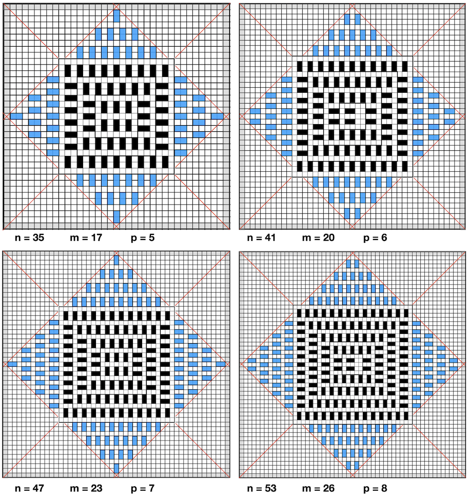
Figure 13: A 4–sequence of $\mathcal{D}_{n}$ expansion in Class $12$. The class of the square core $\mathcal{S}_{f_{12}(m)}$ alternates from $(\dot{12})$ to $(\dot{11})$ (refer to Fig. 9) whereas a new row is added in $\mathcal{W}_{12}$ for $p$ odd.

4.3.2 Capacity and expansion of $\mathcal{D}_{n}$ in Class $12$

The capacity $\psi_{n}$ of $\mathcal{D}_{n}$ in Class $12$ is given by

$$\psi_{n}=\xi_{f_{12}(m)}+4\,W_{12}(p)$$ (39)

and with $W_{12}\equiv W_{10}$ we get

• $\mu_{p}=0\Rightarrow$ from (35) and from (23)

  $$\psi_{n}=\frac{m(m+4)}{6}+\frac{p\,(3\,p+2)}{2}$$

• $\mu_{p}=1\Rightarrow$ from (36) and from (23)

  $$\psi_{n}=\frac{(m+1)^{2}}{6}+\frac{(p+1)\,(3\,p+1)}{2}$$

and finally

$$\psi_{n}=(3p+2)(p+1)=\frac{(n-1)(n+1)}{12}$$ (40)

whatever the parity of $p$.

The expansion rate of $\psi_{n}$ can also be obtained stepwise: it follows from (37–38) and from (22) that is, with $p>0$

$$\psi_{n}-\psi_{n-6}=(\xi_{f_{12}(m)}-\xi_{f_{12}(m-3)})+4\,(W_{12}(p)-W_{12}(p-1))$$

$$=\mu_{p}(2\,p+2)\,+\,(1-\mu_{p})(4\,p+2)\,+2\,p\,(1+\mu_{p})=6\,p+2$$

now $n=2\,m+1$ and $m=3\,p+2$ then

$$\psi_{5}=2\ ;\hskip 5.69054pt\psi_{n}-\psi_{n-6}=n-3\,.$$ (41)

The values of $\psi_{n}$ in Class $12$ are displayed in Table 10. A 4–sequence of expansions is displayed in Fig. 13.

5 Dominos in the Diamond — $n$ even

Again and like for the odd case, the following constructions for $\overline{0\,m}$ classes (or “$0\,m$”) will be valid only when the core–wedge structure actually appears from Fig. 8. Therefore, the same conditions on $p$ will be assumed everywhere. The first configurations with $p=0$ are shown in Fig. 14.

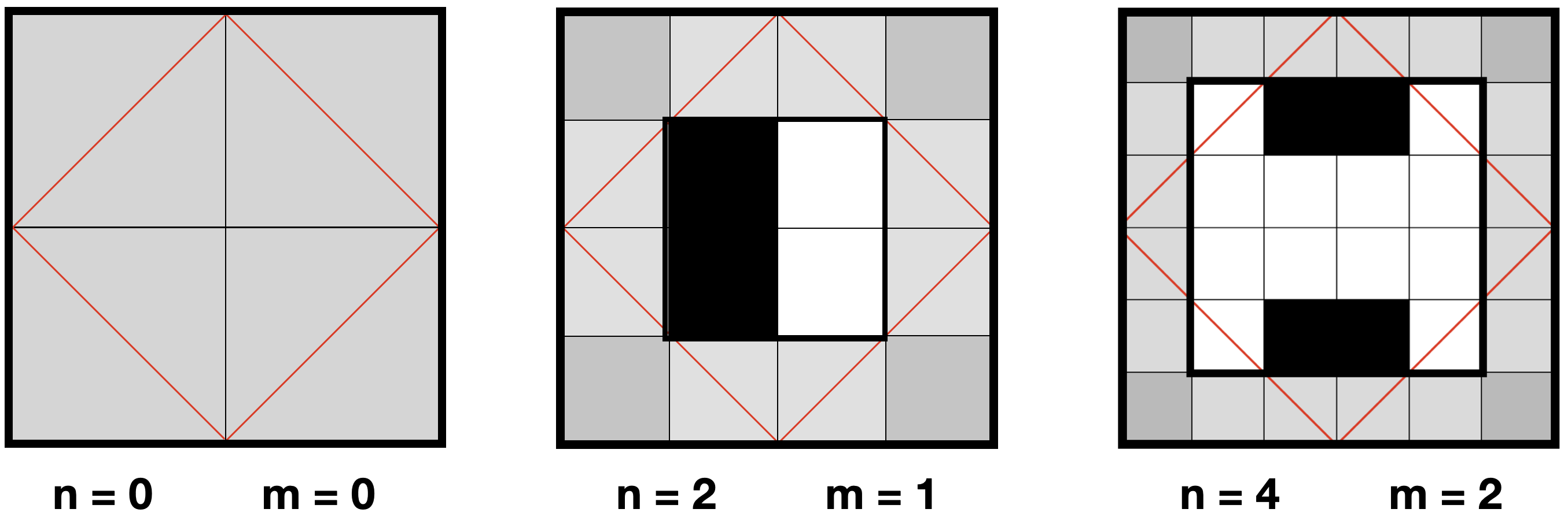
Figure 14: – $n$ even. The first configurations with $p=0$. From left to right: Class ${00}$ ($\psi_{0}=0$), Class ${01}$ ($\psi_{2}=1$), Class ${02}$ ($\psi_{4}=2$).

Whereas the case – $n$ odd – argued for a “vertical” layout (dominos perpendicular to the adjacent core’s side), now the case – $n$ even – argues for a “horizontal” layout (dominos parallel to the adjacent core’s side). Referring back to Fig. 6 (right) the exact size $f_{0m}\approx m$ of the core will be adjusted so that the configuration of the wedges is entirely fixed by the $p$ parameter. Let $f_{0m}^{+}(m)=f_{0m}(m)+2$ be the extended length of the side of $\mathcal{S}_{f_{0m}(m)}$ including borders, and let $h_{0m}$ such that

$$f_{0m}^{+}(m)=n-2\cdot h_{0m}(p)\hskip 28.45274pt(n=2m)$$

where $h_{0m}$ is the height of the vertical median column of Region $\mathcal{W}_{0m}.$ By observing that this wedge is an isosceles right triangle, we fix its height so that

$$2\cdot h_{0m}(p)=m-3+\left\{\begin{array}[]{ll}r_{p+1}&\mbox{ in {Class} $00$ }\\ r_{p}&\mbox{ in {Class} $01$ }\\ r_{p-1}&\mbox{ in {Class} $02$ }\end{array}\right.$$ (42)

$$\mbox{ with }\hskip 5.69054pt\left\{\begin{array}[]{clll}p+1&=4\,q_{p+1}+r_{p+1}&(0\leq r_{p+1}<4)&\mbox{ in {Class} $00$ }\\ p&=4\,q_{p}+r_{p}&(0\leq r_{p}<4)&\mbox{ in {Class} $01$ }\\ p-1&=4\,q_{p-1}+r_{p-1}&(0\leq r_{p-1}<4)&\mbox{ in {Class} $02$ }\\ \end{array}\right.$$ (43)

whence finally the strict length of the side in the square core

$$f_{0m}(m)=f_{0m}^{+}(m)-2=\left\{\begin{array}[]{ll}m+1-r_{p+1}&\mbox{ in {Class} $00$ }\\ m+1-r_{p}&\mbox{ in {Class} $01$ }\\ m+1-r_{p-1}&\mbox{ in {Class} $02$ }\\ \end{array}\right.$$ (44)

expressed in terms of $m$. Or, by using a general unifying notation we get

$$f_{0m}(m)=m+1-r_{\widehat{p}}$$ (45)

$$\widehat{p}=4\,q_{\widehat{p}}+r_{\widehat{p}}\ :\hskip 14.22636pt\widehat{p}=p+1-m\bmod 3\hskip 14.22636pt(0\leq r_{\widehat{p}}<4)$$ (46)

and where the $(q_{\widehat{p}},r_{\widehat{p}})$ are quotient and remainder of dividing by 4 the left–hand term in $p$. Moreover, with $r_{\widehat{p}-1}=(r_{\widehat{p}}-1)\bmod 4$ we get

$$f_{0m}(m)-f_{0m}(m-3)=3-r_{\widehat{p}}+(r_{\widehat{p}}-1)\bmod 4=\left\{\begin{array}[]{ll}+6&\mbox{ for }r_{\widehat{p}}=0\\ +2&\mbox{ otherwise }\end{array}\right.$$ (47)

giving the elongation of the side of the core within a $p-1\rightarrow p$ expansion. The evolution will follow a 4–cycle sequence, namely a “$(q_{\widehat{p}})$–cycle” at constant $q_{\widehat{p}}.$

5.1 Class $00$ — $n$ even   &   $m\equiv 0\pmod{3}$

The basic parameters of Class $00$ verify:

$$p\,\in\,\mathbb{N}\,;\hskip 14.22636ptm\,=3\,p\,;\hskip 14.22636ptn\,=2\,m\,;$$

5.1.1 Capacity and expansion rate of the square core $\mathcal{S}_{f_{00}}$

From (44–46) $f_{00}(m)=m+1-r_{p+1}$ and we get the following four cases

• $r_{p+1}=0\Rightarrow f_{00}(m)=m+1$ and $(m+1)/2\in\dot{2}\hskip 2.84526pt\mbox{in}\hskip 2.84526pt\mathbb{Z}/3\,\mathbb{Z}$ then $\xi_{m+1}$ follows from (13) whence

  $$\xi_{m+1}=\frac{(m+1)(m+3)}{6}$$ (48)

• $r_{p+1}=1\Rightarrow f_{00}(m)=m$ and $m/2\in\dot{0}\hskip 2.84526pt$ then $\xi_{m}$ follows from (11) whence

  $$\xi_{m}=\frac{m(m+2)}{6}$$ (49)

• $r_{p+1}=2\Rightarrow f_{00}(m)=m-1$ and $(m-1)/2\in\dot{1}\hskip 2.84526pt$ then $\xi_{m-1}$ follows from (12) whence

  $$\xi_{m-1}=\frac{(m-1)(m+1)-2}{6}$$ (50)

• $r_{p+1}=3\Rightarrow f_{00}(m)=m-2$ and $(m-2)/2\in\dot{2}\hskip 2.84526pt$ then $\xi_{m-2}$ follows from (13) whence

  $$\xi_{m-2}=\frac{m(m-2)}{6}$$ (51)

giving the capacity of the square core. In the same way, from (47) we get the following four cases

• $r_{p+1}=0\Rightarrow f_{00}(m-3)=f_{00}(m)-6$ whence from (7)

  $$\xi_{m+1}-\xi_{(m+1)-6}=2(m-1)=6\,p-2$$ (52)

• $r_{p+1}=1\Rightarrow f_{00}(m-3)=f_{00}(m)-2=m-2$ and $(m-2)/2\in\dot{2}$ then $\xi_{m-2}$ follows from (13) whence

  $$\xi_{m}-\xi_{m-2}=\frac{m(m+2)}{6}-\frac{m(m-2)}{6}=2\,p$$ (53)

• $r_{p+1}=2\Rightarrow f_{00}(m-3)=f_{00}(m)-2=m-3$ and $(m-3)/2\in\dot{0}$ then $\xi_{m-3}$ follows from (11) whence

  $$\xi_{m-1}-\xi_{m-3}=\frac{(m-1)(m+1)-2}{6}-\frac{(m-3)(m-1)}{6}=2\,p-1$$ (54)

• $r_{p+1}=3\Rightarrow f_{00}(m-3)=f_{00}(m)-2=m-4$ and $(m-4)/2\in\dot{1}$ then $\xi_{m-4}$ follows from (12) whence

  $$\xi_{m-2}-\xi_{m-4}=\frac{m(m-2)}{6}-\frac{(m-4)(m-2)-2}{6}=2\,p-1$$ (55)

giving the expansion rate for the capacity in the square core.

5.1.2 Capacity and expansion rate of the wedge $\mathcal{W}_{00}$

Let $W_{00}(p)$ be the capacity of the wedge for any given $p$. From (42) comes

$$2\,(h_{00}(p)+1)=m-1+\left\{\begin{array}[]{ll}r_{p+1}&\mbox{ in {Class} $00$ }\\ r_{p}&\mbox{ in {Class} $01$ }\\ r_{p-1}&\mbox{ in {Class} $02$ }\end{array}\right.$$

and thus we get the capacity of the vertical median of Region $\mathcal{W}_{00}$

$$\overline{h}_{00}(p)=(h_{00}(p)+1)/2=\frac{1}{4}\,(3\,p-1+r_{p+1})$$

in number of horizontal dominos – namely, in number of horizontal rows of dominos. From (43) let us bring out the entity $p-q_{p+1}$ as

$$p-q_{p+1}=3\,q_{p+1}+(r_{p+1}-1)\hskip 5.69054pt\mbox{or}\hskip 5.69054pt4\,(p-q_{p+1})=3\,p+(r_{p+1}-1)$$ (56)

by eliminating the $q_{p+1}$ term from the second member. It follows that

$$\overline{h}_{00}(p)=p-q_{p+1}\hskip 8.53581pt\mbox{whence}\hskip 8.53581pt\overline{h}_{00}(p)-\overline{h}_{00}(p-1)=\left\{\begin{array}[]{ll}0&\mbox{ if }r_{p+1}=0\\ +1&\mbox{ otherwise }\end{array}\right.$$ (57)

and as a result, the number of rows increases within each internal step and remains constant at the start of a new cycle. The baserow of the N–wedge has the length

$$b_{00}(p)=2\cdot h_{00}(p)=3\,p+r_{p+1}-3$$

rewritten as the sum $b_{00}(p)=b^{\prime}_{00}(p)+b^{\prime\prime}_{00}(p)$ with

$$b^{\prime}_{00}(p)=3\,(p-q_{p+1})\hskip 5.69054pt\mbox{and}\hskip 5.69054ptb^{\prime\prime}_{00}(p)=3\,(q_{p+1}-1)+r_{p+1}\hskip 14.22636pt(p>1)$$ (58)

that yields $\overline{b}_{00}(p)=\overline{b^{\prime}}_{00}(p)+\overline{b^{\prime\prime}}_{00}(p)$ where $\overline{b}_{00}$ is the capacity in terms of (horizontal) dominos of the baserow of Region $\mathcal{W}_{00}$ and where $\overline{b^{\prime}}_{00}\hskip 2.84526pt\mbox{and}\hskip 2.84526pt\overline{b^{\prime\prime}}_{00}$ denote the capacity of the baserow of $\mathcal{W}^{\prime}_{00}\hskip 2.84526pt\mbox{and}\hskip 2.84526pt\mathcal{W}^{\prime\prime}_{00}$ respectively.

Capacity and expansion of the subwedge $\mathcal{W}^{\prime}_{00}$.

Regarding $\mathcal{W}^{\prime}_{00}$ it follows that

$$\overline{b^{\prime}}_{00}(p)=\frac{1}{3}\,\cdot\,b^{\prime}_{00}(p)=p-q_{p+1}=\overline{h}_{00}(p)$$ (59)

and $\overline{b^{\prime}}_{00}$ behaves like $\overline{h^{\prime}}_{00}$ in (57). Now $W^{\prime}_{00}(0)=0$ and from (57) and (59)

$$W^{\prime}_{00}(p)-W^{\prime}_{00}(p-1)=\left\{\begin{array}[]{ll}0&\mbox{ if }r_{p+1}=0\\ p-q_{p+1}&\mbox{ otherwise }\end{array}\right.$$ (60)

and with

$$W^{\prime}_{00}(p)=\sum_{k=1}^{p-q_{p+1}}k=(p-q_{p+1})\,(p-q_{p+1}+1)/2$$ (61)

we finally obtain the total capacity of Region $\mathcal{W}^{\prime}_{00}.$ Or expressed in another way

$$W^{\prime}_{0m}(p)-W^{\prime}_{0m}(p-1)=\left\{\begin{array}[]{ll}0&\mbox{ if }r_{\widehat{p}}=0\\ \overline{b^{\prime}}_{0m}(p)=p-q_{\widehat{p}}&\mbox{ otherwise }\end{array}\right.$$ (62)

$$W^{\prime}_{0m}(p)=(p-q_{\widehat{p}})\,(p-q_{\widehat{p}}+1)/2$$ (63)

$$4\cdot W^{\prime}_{0m}(p)=2\,(p-q_{\widehat{p}})\,(p-q_{\widehat{p}}+1)$$ (64)

now without $m$–class–aware statement. In Class $00$, from (56) and (61) it comes now

$$4\cdot W^{\prime}_{00}(p)=\frac{(3\,p+r_{p+1}-1)(3\,p+r_{p+1}+3)}{8}$$

whence

$$4\cdot W^{\prime}_{00}(p)=\left\{\begin{array}[]{ll}(3\,p-1)(3\,p+3)/8&\mbox{ if }r_{p+1}=0\\ (3\,p)(3\,p+4)/8&\mbox{ if }r_{p+1}=1\\ (3\,p+1)(3\,p+5)/8&\mbox{ if }r_{p+1}=2\\ (3\,p+2)(3\,p+6)/8&\mbox{ if }r_{p+1}=3\\ \end{array}\right.$$ (65)

giving the overall capacity of the four N–S–E–W subregions $\mathcal{W}^{\prime}_{00}$ in terms of $p$.

Capacity and expansion of the subwedge $\mathcal{W}^{\prime\prime}_{00}$.

From (58) we get

$$\overline{b^{\prime\prime}}_{00}(p)=(q_{p+1}-1)+\delta_{r_{p+1}}\hskip 8.53581pt\mbox{with}\hskip 8.53581pt\delta_{r_{p+1}}=\Bigl{\lfloor}\,\frac{r_{p+1}\,}{3}\Bigr{\rceil}$$ (66)

where the second term on the right side denotes the integer rounding closest to the rational $r_{p+1}/3$. Region $\mathcal{W}^{\prime\prime}_{00}$ is empty for $p=1$ then for any $p>1$

$$W^{\prime\prime}_{00}(p)-W^{\prime\prime}_{00}(p-1)=\left\{\begin{array}[]{ll}0&\mbox{ if }r_{p+1}=0\\ q_{p+1}-1+\delta_{r_{p+1}}&\mbox{ otherwise. }\end{array}\right.$$ (67)

The periodic sequence of expansion within a $q_{p+1}$–cycle (at constant $q_{p+1}$) is as follows:

• $r_{p+1}=0$, $\delta_{r_{p+1}}=0\Rightarrow W^{\prime\prime}_{00}(p)=W^{\prime\prime}_{00}(p-1)$ and the baserow can accommodate exactly $q_{p+1}-1$ dominos.

• $r_{p+1}=1$, $\delta_{r_{p+1}}=0\Rightarrow W^{\prime\prime}_{00}(p)=W^{\prime\prime}_{00}(p-1)+q_{p+1}-1$ and a new lacunar void is inserted in the new baserow.

• $r_{p+1}=2$, $\delta_{r_{p+1}}=1\Rightarrow W^{\prime\prime}_{00}(p)=W^{\prime\prime}_{00}(p-1)+q_{p+1}$ and a new domino is inserted in the new baserow.

• $r_{p+1}=3$, $\delta_{r_{p+1}}=1\Rightarrow W^{\prime\prime}_{00}(p)=W^{\prime\prime}_{00}(p-1)+q_{p+1}$ and a new baserow of the same capacity is added.

By adding up all items, the expansion in $\mathcal{W}^{\prime\prime}_{00}$ at the end of the $q_{p+1}$–cycle becomes $3\,q_{p+1}-1.$ Now, at the end of the first cycle $W^{\prime\prime}_{00}(2)=0$ and with $r_{p+1}=3$ we can get

$$W^{\prime\prime}_{00}(p)=\sum_{k=1}^{q_{p+1}}(3\,k-1)=\frac{q_{p+1}\,(3\,q_{p+1}+1)}{2}$$ (68)

and subtracting step by step back

$$W^{\prime\prime}_{00}(p)=\left\{\begin{array}[]{ll}q_{p+1}\,(3\,q_{p+1}+1)/2&\mbox{ if }r_{p+1}=3\\ q_{p+1}\,(3\,q_{p+1}-1)/2&\mbox{ if }r_{p+1}=2\\ (q_{p+1}-1)\,3\,q_{p+1}/2&\mbox{ if }r_{p+1}=1\\ (q_{p+1}-1)\,(3\,q_{p+1}-2)/2&\mbox{ if }r_{p+1}=0\end{array}\right.$$ (69)

or even in the form

$$W^{\prime\prime}_{00}(p)=\overline{b^{\prime\prime}}_{00}(p)\cdot\frac{(p-q_{p+1}-3)+(p-q_{p+1}-3\cdot\overline{b^{\prime\prime}}_{00}(p))}{2}$$ (70)

in order to get rid of the dependence of $W^{\prime\prime}_{00}$ on $r_{p+1}$ and also to emphasize that $W^{\prime\prime}_{00}$ grows with the area of Triangle $\mathcal{W}^{\prime\prime}_{00}.$ Or in another way, from (66) comes

$$\overline{b^{\prime\prime}}_{0m}(p)=(q_{\widehat{p}}-1)+\delta_{r_{\widehat{p}}}\hskip 8.53581pt\mbox{with}\hskip 8.53581pt\delta_{r_{\widehat{p}}}=\Bigl{\lfloor}\,\frac{r_{\widehat{p}}+m\bmod 3\,}{3}\Bigr{\rceil}$$ (71)

then from (67) and (70) we get

$$W^{\prime\prime}_{0m}(p)-W^{\prime\prime}_{0m}(p-1)=\left\{\begin{array}[]{ll}0&\mbox{ if }r_{\widehat{p}}=0\\ \overline{b^{\prime\prime}}_{0m}(p)=q_{\widehat{p}}-1+\delta_{r_{\widehat{p}}}&\mbox{ otherwise }\end{array}\right.$$ (72)

$$W^{\prime\prime}_{0m}(p)=\overline{b^{\prime\prime}}_{0m}(p)\cdot\frac{(p-q_{\widehat{p}}-3)+(p-q_{\widehat{p}}-3\cdot\overline{b^{\prime\prime}}_{0m}(p))}{2}$$ (73)

$$4\cdot W^{\prime\prime}_{0m}(p)=2\cdot\overline{b^{\prime\prime}}_{0m}(p)\cdot((p-q_{\widehat{p}}-3)+(p-q_{\widehat{p}}-3\cdot\overline{b^{\prime\prime}}_{0m}(p)))$$ (74)

now expressed according to a $m$–class–unaware statement. In Class $00$, substituting $q_{p+1}=(p+1-r_{p+1})/4$ from (43) in (69) it comes now

$$4\cdot W^{\prime\prime}_{00}(p)=\left\{\begin{array}[]{ll}(p-3)(3p-5)/8&\mbox{ if }r_{p+1}=0\\ (p-4)(3p)/8&\mbox{ if }r_{p+1}=1\\ (p-1)(3p-7)/8&\mbox{ if }r_{p+1}=2\\ (p-2)(3p-2)/8&\mbox{ if }r_{p+1}=3\\ \end{array}\right.$$ (75)

giving the overall capacity of the four N–S–E–W subregions $\mathcal{W}^{\prime\prime}_{00}$ in terms of $p$.

5.1.3 Capacity and expansion of $\mathcal{D}_{n}$ in Class $00$

The capacity $\psi_{n}$ of $\mathcal{D}_{n}$ in Class $00$ is simply given by

$$\psi_{n}=\xi_{f_{00}(m)}+4\,(W^{\prime}_{00}(p)+W^{\prime\prime}_{00}(p))$$ (76)

then from (48)–(51) for $\xi_{f_{00}(m)}$ and from (65) and (75) for $W^{\prime}_{00}(p)$ and $W^{\prime\prime}_{00}(p)$ it would easily come

$$\psi_{n}=\left\{\begin{array}[]{ll}(n^{2}+2n+24)/12&\mbox{ if }r_{p+1}=0\\ (n^{2}+2n)/12&\mbox{ if }r_{p+1}=1\\ (n^{2}+2n+12)/12&\mbox{ if }r_{p+1}=2\\ (n^{2}+2n+24)/12&\mbox{ if }r_{p+1}=3\\ \end{array}\right.$$ (77)

with $m=3p$ and $n=2m$. With $\psi_{0}=0$ the expansion rate of $\psi_{n}$ can also be obtained stepwise. In Tab. 1, the sum of the three terms resulting from relations (52–55) for $\Delta\xi_{f_{00}(m)},$ from (60) for $\Delta W^{\prime}_{00}(p)$ and from (67) for $\Delta W^{\prime\prime}_{00}(p)$ gives the result. Moreover, by adding backwards the four terms in the last column of Tab. 1, it follows that

$$\psi_{n}-\psi_{n-24}=(n-2)+((n-6)-1)+((n-12)-1)+((n-18)-4)$$

$=4\,n-(\,2+7+13+22\,)$ whence the induction

$$\psi_{0}=0\,;\hskip 5.69054pt\psi_{n}=\psi_{n-24}\ +4\,(n-11)\hskip 14.22636pt(p\geq 4)$$ (78)

within any $p\rightarrow p+4$ cycle.

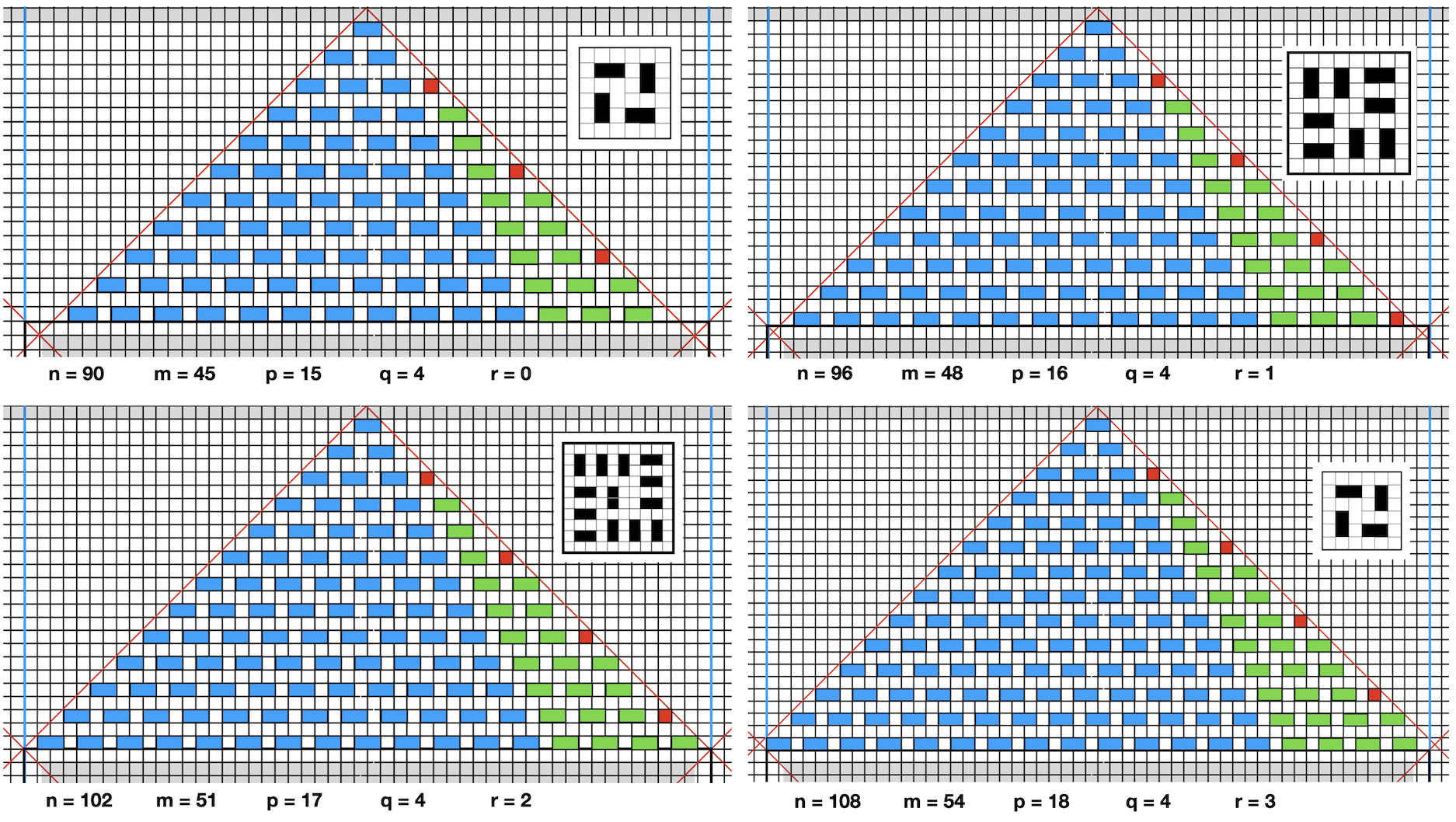
Figure 15: A 4–sequence of $\mathcal{D}_{n}$ expansion in Class $00$. The class of the square core $\mathcal{S}_{f_{00}(m)}$ (refer to Fig. 9) evolves as $(\dot{02})\rightarrow(\dot{00})\rightarrow(\dot{01})\rightarrow(\dot{02})$ (highlighted in insets). A new sequence starts with $p+1\equiv_{4}0$ whereas $\mathcal{W}_{00}$ remains unchanged.

Table 1: Expansion in Class $00$: $p\,\in\,\mathbb{N}\,;m\,=3\,p\,;n\,=2\,m\,;\ -\ \hskip 2.84526pt\psi_{0}=0\,;\newline \mbox{ }\hskip 36.98857ptr_{p+1}\equiv p+1\pmod{4}$

$r_{p+1}$	$\Delta\xi_{f_{00}(m)}$	$4\,\Delta W^{\prime}_{00}(p)$	$4\,\Delta W^{\prime\prime}_{00}(p)$	$\psi_{n}-\psi_{n-6}$
0	$6\,p-2$	$0$	$0$	$n-2$
1	$2\,p$	$4\,(p-q_{p+1})$	$4\,(q_{p+1}-1)$	$n-4$
2	$2\,p-1$	$4\,(p-q_{p+1})$	$4\,q_{p+1}$	$n-1$
3	$2\,p-1$	$4\,(p-q_{p+1})$	$4\,q_{p+1}$	$n-1$

A 4–sequence of expansion is illustrated in Fig. 15. The values of $\psi_{n}$ in Class $00$ are displayed in Table 11.

5.2 Class $01$ — $n$ even   &   $m\equiv 1\pmod{3}$

The basic parameters of Class $01$ verify:

$$p\,\in\,\mathbb{N}\,;\hskip 14.22636ptm\,=3\,p\,+\,1\,;\hskip 14.22636ptn\,=2\,m\,;$$

5.2.1 Capacity and expansion rate of the square core $\mathcal{S}_{f_{01}}$

From (44–46) $f_{01}(m)=m+1-r_{p}$ and we get the following four cases

• $r_{p}=0\Rightarrow f_{01}(m)=m+1$ and $(m+1)/2\in\dot{1}\hskip 2.84526pt\mbox{in}\hskip 2.84526pt\mathbb{Z}/3\,\mathbb{Z}$ then $\xi_{m+1}$ follows from (12) whence

  $$\xi_{m+1}=\frac{(m+1)(m+3)-2}{6}$$ (79)

• $r_{p}=1\Rightarrow f_{01}(m)=m$ and $m/2\in\dot{2}\hskip 2.84526pt$ then $\xi_{m}$ follows from (13) whence

  $$\xi_{m}=\frac{m(m+2)}{6}$$ (80)

• $r_{p}=2\Rightarrow f_{01}(m)=m-1$ and $(m-1)/2\in\dot{0}\hskip 2.84526pt$ then $\xi_{m-1}$ follows from (11) whence

  $$\xi_{m-1}=\frac{(m-1)(m+1)}{6}$$ (81)

• $r_{p}=3\Rightarrow f_{01}(m)=m-2$ and $(m-2)/2\in\dot{1}\hskip 2.84526pt$ then $\xi_{m-2}$ follows from (12) whence

  $$\xi_{m-2}=\frac{m(m-2)-2}{6}$$ (82)

giving the capacity of the square core. In the same way, from (47) we get the following four cases

• $r_{p}=0\Rightarrow f_{01}(m-3)=f_{01}(m)-6$ whence from (7)

  $$\xi_{m+1}-\xi_{(m+1)-6}=2(m-1)=6\,p$$ (83)

• $r_{p}=1\Rightarrow f_{01}(m-3)=f_{01}(m)-2=m-2$ and $(m-2)/2\in\dot{1}$ then $\xi_{m-2}$ follows from (12) whence

  $$\xi_{m}-\xi_{m-2}=\frac{m(m+2)}{6}-\frac{m(m-2)-2}{6}=2\,p+1$$ (84)

• $r_{p}=2\Rightarrow f_{01}(m-3)=f_{01}(m)-2=m-3$ and $(m-3)/2\in\dot{2}$ then $\xi_{m-3}$ follows from (13) whence

  $$\xi_{m-1}-\xi_{m-3}=\frac{(m-1)(m+1)}{6}-\frac{(m-3)(m-1)}{6}=2\,p$$ (85)

• $r_{p}=3\Rightarrow f_{01}(m-3)=f_{01}(m)-2=m-4$ and $(m-4)/2\in\dot{0}$ then $\xi_{m-4}$ follows from (11) whence

  $$\xi_{m-2}-\xi_{m-4}=\frac{m(m-2)-2}{6}-\frac{(m-4)(m-2)}{6}=2\,p-1$$ (86)

giving the expansion rate for the capacity in the square core.

5.2.2 Capacity and expansion of $\mathcal{D}_{n}$ in Class $01$

The capacity $\psi_{n}$ of $\mathcal{D}_{n}$ in Class $01$ is simply given by

$$\psi_{n}=\xi_{f_{01}(m)}+4\,(W^{\prime}_{01}(p)+W^{\prime\prime}_{01}(p))$$ (87)

and $\xi_{f_{01}(m)}$ results from (79)–(82). In Class $01$ from (43) it comes

$$p-q_{p}=3\,q_{p}+r_{p}\hskip 5.69054pt\mbox{or}\hskip 5.69054pt4\,(p-q_{p})=3\,p+r_{p}$$ (88)

and from (64)

$$W^{\prime}_{01}(p)=(p-q_{p})\,(p-q_{p}+1)/2$$ (89)

rewritten from (88) as

$$4\cdot W^{\prime}_{01}(p)=\frac{(3\,p+r_{p})(3\,p+r_{p}+4)}{8}$$

whence

$$4\cdot W^{\prime}_{01}(p)=\left\{\begin{array}[]{ll}(3\,p)(3\,p+4)/8&\mbox{ if }r_{p}=0\\ (3\,p+1)(3\,p+5)/8&\mbox{ if }r_{p}=1\\ (3\,p+2)(3\,p+6)/8&\mbox{ if }r_{p}=2\\ (3\,p+3)(3\,p+7)/8&\mbox{ if }r_{p}=3\\ \end{array}\right.$$ (90)

giving the overall capacity of the four N–S–E–W subregions $\mathcal{W}^{\prime}_{01}$ in terms of $p$.

For subregion $\mathcal{W}^{\prime\prime}_{01}$ we get

$$\overline{b^{\prime\prime}}_{01}(p)=(q_{p}-1)+\delta_{r_{p}}\hskip 8.53581pt\mbox{with}\hskip 8.53581pt\delta_{r_{p}}=\Bigl{\lfloor}\,\frac{r_{p}+1\,}{3}\Bigr{\rceil}$$ (91)

$$W^{\prime\prime}_{01}(p)=\overline{b^{\prime\prime}}_{01}(p)\cdot\frac{(p-q_{p}-3)+(p-q_{p}-3\cdot\overline{b^{\prime\prime}}_{01}(p))}{2}$$ (92)

from (71) and (74) respectively. It follows that

$$\overline{b^{\prime\prime}}_{01}(p)=\left\{\begin{array}[]{ll}q_{p}-1&\mbox{ if }r_{p}=0\\ q_{p}&\mbox{ otherwise }\\ \end{array}\right.$$

and then

$$W^{\prime\prime}_{01}(p)=\left\{\begin{array}[]{ll}(q_{p}-1)\cdot(2\,p-5\,q_{p})/2&\mbox{ if }r_{p}=0\\ q_{p}\cdot(2\,p-5\,q_{p}-3)/2&\mbox{ otherwise. }\\ \end{array}\right.$$

Replacing $q_{p}$ by $(p-r_{p})/4$ from (43) it comes

$$4\cdot W^{\prime\prime}_{01}(p)=\left\{\begin{array}[]{ll}(p-r_{p}-4)\cdot(3\,p+5\,r_{p})/8&\mbox{ if }r_{p}=0\\ (p-r_{p})\cdot(3\,p+5\,r_{p}-12)/8&\mbox{ otherwise }\\ \end{array}\right.$$

whence

$$4\cdot W^{\prime\prime}_{01}(p)=\left\{\begin{array}[]{ll}3p\,(p-4)/8&\mbox{ if }r_{p}=0\\ (p-1)(3p-7)/8&\mbox{ if }r_{p}=1\\ (p-2)(3p-2)/8&\mbox{ if }r_{p}=2\\ (p-3)(3p+3)/8&\mbox{ if }r_{p}=3\end{array}\right.$$ (93)

giving the overall capacity of the four N–S–E–W subregions $\mathcal{W}^{\prime\prime}_{01}$ in terms of $p$.

Finally, from (79)–(82) for $\xi_{f_{01}(m)}$ and from (90) and (93) for $W^{\prime}_{01}(p)$ and $W^{\prime\prime}_{01}(p)$ it would easily come

$$\psi_{n}=\left\{\begin{array}[]{ll}(n^{2}+2n+4)/12&\mbox{ if }r_{p}=0\\ (n^{2}+2n+16)/12&\mbox{ if }r_{p}=1\\ (n^{2}+2n+16)/12&\mbox{ if }r_{p}=2\\ (n^{2}+2n+4)/12&\mbox{ if }r_{p}=3\end{array}\right.$$ (94)

with $m=3p+1$ and $n=2m$. With $\psi_{2}=1$ the expansion rate of $\psi_{n}$ can also be obtained stepwise. From (62) and (72) it comes

$$W^{\prime}_{01}(p)-W^{\prime}_{01}(p-1)=\left\{\begin{array}[]{ll}0&\mbox{ if }r_{p}=0\\ p-q_{p}&\mbox{ otherwise }\end{array}\right.$$ (95)

$$W^{\prime\prime}_{01}(p)-W^{\prime\prime}_{01}(p-1)=\left\{\begin{array}[]{ll}0&\mbox{ if }r_{p}=0\\ q_{p}-1+\delta_{r_{p}}=q_{p}&\mbox{ otherwise }\end{array}\right.$$ (96)

and in Tab. 2, the sum of the three terms resulting from relations (83–86) for $\Delta\xi_{f_{01}(m)},$ from (95) for $\Delta W^{\prime}_{01}(p)$ and from (96) for $\Delta W^{\prime\prime}_{01}(p)$ gives the result. Moreover, by adding backwards the four terms in the last column of Tab. 2, it follows that

$$\psi_{n}-\psi_{n-24}=(n-2)+((n-6)-3)+((n-12)-2)+((n-18)-1)$$

$=4\,n-(\,2+9+14+19\,)$ whence the induction

$$\psi_{2}=1\,;\hskip 5.69054pt\psi_{n}=\psi_{n-24}\ +4\,(n-11)\hskip 14.22636pt(p\geq 4)$$ (97)

within any $p\rightarrow p+4$ cycle. A 4–sequence of expansion is illustrated in Fig. 16.

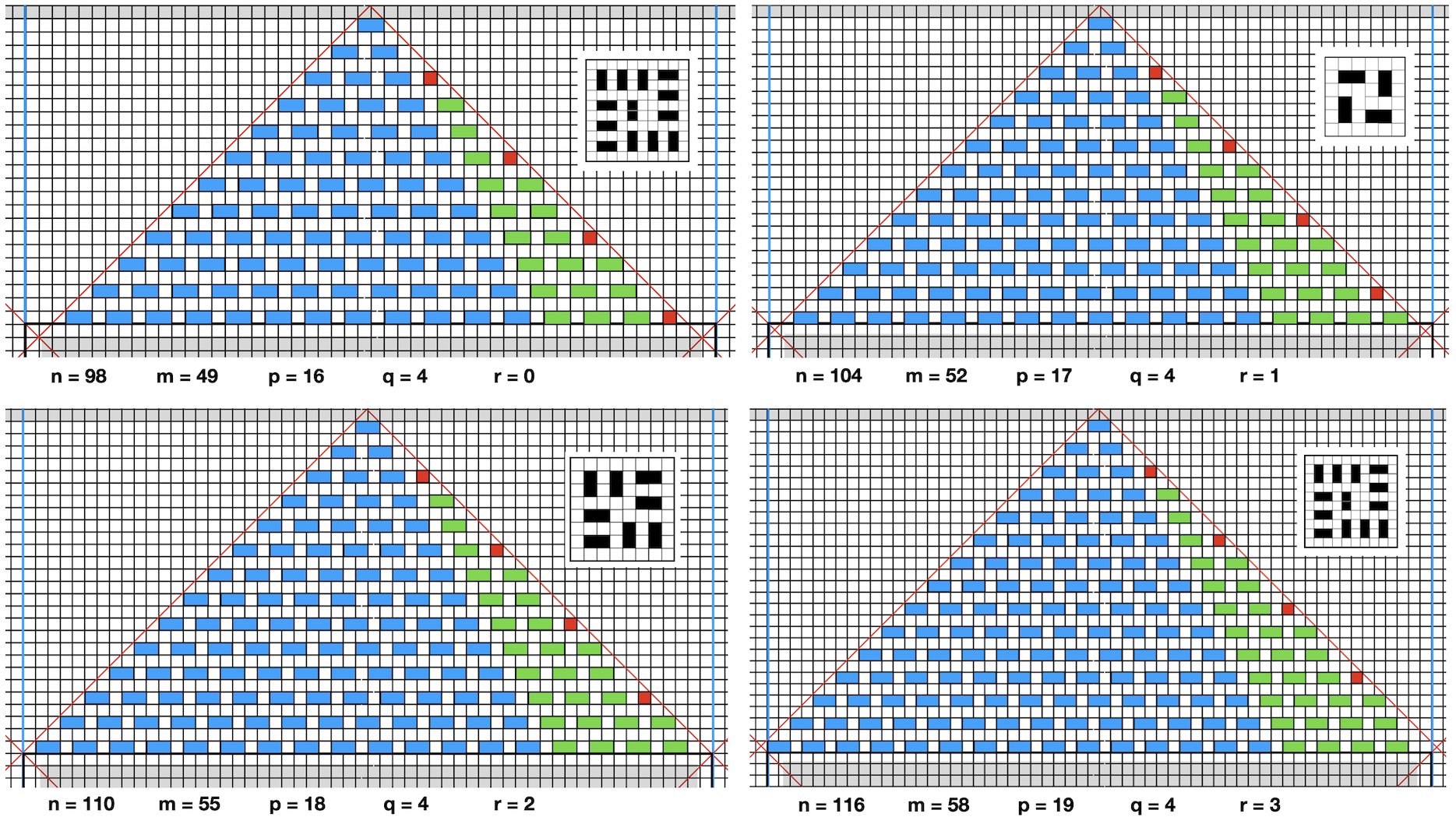
Figure 16: A 4–sequence of $\mathcal{D}_{n}$ expansion in Class $01$. The class of the square core $\mathcal{S}_{f_{01}(m)}$ (refer to Fig. 9) evolves as $(\dot{01})\rightarrow(\dot{02})\rightarrow(\dot{00})\rightarrow(\dot{01})$ (highlighted in insets). A new sequence starts with $p\equiv_{4}0$ whereas $\mathcal{W}_{01}$ remains unchanged.

The values of $\psi_{n}$ in Class $01$ are displayed in Table 12.

Table 2: Expansion in Class $01$: $p\,\in\,\mathbb{N}\,;m\,=3\,p+1\,;n\,=2\,m\,;\ -\ \hskip 2.84526pt\psi_{2}=1\,;\newline \mbox{ }\hskip 36.98857ptr_{p}\equiv p\pmod{4}$

$r_{p}$	$\Delta\xi_{f_{01}(m)}$	$4\,\Delta W^{\prime}_{01}(p)$	$4\,\Delta W^{\prime\prime}_{01}(p)$	$\psi_{n}-\psi_{n-6}$
0	$6\,p$	$0$	$0$	$n-2$
1	$2\,p+1$	$4\,(p-q_{p})$	$4\,q_{p}$	$n-1$
2	$2\,p$	$4\,(p-q_{p})$	$4\,q_{p}$	$n-2$
3	$2\,p-1$	$4\,(p-q_{p})$	$4\,q_{p}$	$n-3$

5.3 Class $02$ — $n$ even   &   $m\equiv 2\pmod{3}$

The basic parameters of Class $02$ verify:

$$p\,\in\,\mathbb{N}\,;\hskip 14.22636ptm\,=3\,p\,+\,2\,;\hskip 14.22636ptn\,=2\,m\,;$$

5.3.1 Capacity and expansion rate of the square core $\mathcal{S}_{f_{02}}$

From (44–46) $f_{02}(m)=m+1-r_{p-1}$ and we get the following four cases

• $r_{p-1}=0\Rightarrow f_{02}(m)=m+1$ and $(m+1)/2\in\dot{0}\hskip 2.84526pt\mbox{in}\hskip 2.84526pt\mathbb{Z}/3\,\mathbb{Z}$ then $\xi_{m+1}$ follows from (11) whence

  $$\xi_{m+1}=\frac{(m+1)\,(m+3)}{6}$$ (98)

• $r_{p-1}=1\Rightarrow f_{02}(m)=m$ and $m/2\in\dot{1}\hskip 2.84526pt$ then $\xi_{m}$ follows from (12) whence

  $$\xi_{m}=\frac{m(m+2)-2}{6}$$ (99)

• $r_{p-1}=2\Rightarrow f_{02}(m)=m-1$ and $(m-1)/2\in\dot{2}\hskip 2.84526pt$ then $\xi_{m-1}$ follows from (13) whence

  $$\xi_{m-1}=\frac{(m-1)(m+1)}{6}$$ (100)

• $r_{p-1}=3\Rightarrow f_{02}(m)=m-2$ and $(m-2)/2\in\dot{0}\hskip 2.84526pt$ then $\xi_{m-2}$ follows from (11) whence

  $$\xi_{m-2}=\frac{m(m-2)}{6}$$ (101)

giving the capacity of the square core. In the same way, from (47) we get the following four cases

• $r_{p+1}=0\Rightarrow f_{02}(m-3)=f_{02}(m)-6$ whence from (7)

  $$\xi_{m+1}-\xi_{(m+1)-6}=2(m-1)=6\,p+2$$ (102)

• $r_{p-1}=1\Rightarrow f_{02}(m-3)=f_{02}(m)-2=m-2$ and $(m-2)/2\in\dot{0}$ then $\xi_{m-2}$ follows from (11) whence

  $$\xi_{m}-\xi_{m-2}=\frac{m(m+2)-2}{6}-\frac{m(m-2)}{6}=2\,p+1$$ (103)

• $r_{p-1}=2\Rightarrow f_{02}(m-3)=f_{02}(m)-2=m-3$ and $(m-3)/2\in\dot{1}$ then $\xi_{m-3}$ follows from (12) whence

  $$\xi_{m-1}-\xi_{m-3}=\frac{(m-1)(m+1)}{6}-\frac{(m-3)(m-1)-2}{6}=2\,p+1$$ (104)

• $r_{p-1}=3\Rightarrow f_{02}(m-3)=f_{02}(m)-2=m-4$ and $(m-4)/2\in\dot{2}$ then $\xi_{m-4}$ follows from (13) whence

  $$\xi_{m-2}-\xi_{m-4}=\frac{m(m-2)}{6}-\frac{(m-4)(m-2)}{6}=2\,p$$ (105)

giving the expansion rate for the capacity in the square core.

5.3.2 Capacity and expansion of $\mathcal{D}_{n}$ in Class $02$

The capacity $\psi_{n}$ of $\mathcal{D}_{n}$ in Class $02$ is simply given by

$$\psi_{n}=\xi_{f_{02}(m)}+4\,(W^{\prime}_{02}(p)+W^{\prime\prime}_{02}(p))$$ (106)

and $\xi_{f_{02}(m)}$ results from (98)–(101). In Class $02$ from (43) it comes

$$p-q_{p-1}=3\,q_{p-1}+r_{p-1}+1\hskip 5.69054pt\mbox{or}\hskip 5.69054pt4\,(p-q_{p-1})=3\,p+r_{p-1}+1$$ (107)

and from (64)

$$W^{\prime}_{02}(p)=(p-q_{p-1})\,(p-q_{p-1}+1)/2$$ (108)

rewritten from (107) as

$$4\cdot W^{\prime}_{02}(p)=\frac{(3\,p+r_{p-1}+1)(3\,p+r_{p-1}+5)}{8}$$

whence

$$4\cdot W^{\prime}_{02}(p)=\left\{\begin{array}[]{ll}(3\,p+1)(3\,p+5)/8&\mbox{ if }r_{p-1}=0\\ (3\,p+2)(3\,p+6)/8&\mbox{ if }r_{p-1}=1\\ (3\,p+3)(3\,p+7)/8&\mbox{ if }r_{p-1}=2\\ (3\,p+4)(3\,p+8)/8&\mbox{ if }r_{p-1}=3\\ \end{array}\right.$$ (109)

giving the overall capacity of the four N–S–E–W subregions $\mathcal{W}^{\prime}_{02}$ in terms of $p$.

For subregion $\mathcal{W}^{\prime\prime}_{02}$ we get

$$\overline{b^{\prime\prime}}_{02}(p)=(q_{p-1}-1)+\delta_{r_{p-1}}\hskip 8.53581pt\mbox{with}\hskip 8.53581pt\delta_{r_{p-1}}=\Bigl{\lfloor}\,\frac{r_{p-1}+2\,}{3}\Bigr{\rceil}$$ (110)

$$W^{\prime\prime}_{02}(p)=\overline{b^{\prime\prime}}_{02}(p)\cdot\frac{(p-q_{p-1}-3)+(p-q_{p-1}-3\cdot\overline{b^{\prime\prime}}_{02}(p))}{2}$$ (111)

from (71) and (74) respectively. It follows that

$$\overline{b^{\prime\prime}}_{02}(p)=\left\{\begin{array}[]{ll}q_{p-1}+1&\mbox{ if }r_{p-1}=3\\ q_{p-1}&\mbox{ otherwise }\\ \end{array}\right.$$

and then

$$W^{\prime\prime}_{02}(p)=\left\{\begin{array}[]{ll}(q_{p-1}+1)\cdot(2\,p-5\,q_{p-1}-6)/2&\mbox{ if }r_{p-1}=3\\ q_{p-1}\cdot(2\,p-5\,q_{p-1}-3)/2&\mbox{ otherwise. }\\ \end{array}\right.$$

Replacing $q_{p-1}$ by $(p-1-r_{p-1})/4$ from (43) it comes

$$4\cdot W^{\prime\prime}_{02}(p)=\left\{\begin{array}[]{ll}p\cdot(3\,p-4)/8&\mbox{ if }r_{p-1}=3\\ (p-1-r_{p-1})\cdot(3\,p+5\,(1+r_{p-1})-12)/8&\mbox{ otherwise }\\ \end{array}\right.$$

whence

$$4\cdot W^{\prime\prime}_{02}(p)=\left\{\begin{array}[]{ll}(p-1)(3p-7)/8&\mbox{ if }r_{p-1}=0\\ (p-2)(3p-2)/8&\mbox{ if }r_{p-1}=1\\ (p-3)(3p+3)/8&\mbox{ if }r_{p-1}=2\\ p\,(3\,p-4)/8&\mbox{ if }r_{p-1}=3\end{array}\right.$$ (112)

giving the overall capacity of the four N–S–E–W subregions $\mathcal{W}^{\prime\prime}_{02}$ in terms of $p$.

Finally, from (98)–(101) for $\xi_{f_{02}(m)}$ and from (109) and (112) for $W^{\prime}_{02}(p)$ and $W^{\prime\prime}_{02}(p)$ it would easily come

$$\psi_{n}=\left\{\begin{array}[]{ll}(n^{2}+2n+24)/12&\mbox{ if }r_{p-1}=0\\ (n^{2}+2n+12)/12&\mbox{ if }r_{p-1}=1\\ (n^{2}+2n)/12&\mbox{ if }r_{p-1}=2\\ (n^{2}+2n+24)/12&\mbox{ if }r_{p-1}=3\end{array}\right.$$ (113)

with $m=3p+2$ and $n=2m$. With $\psi_{4}=2$ the expansion rate of $\psi_{n}$ can also be obtained stepwise. From (62) and (72) it comes

$$W^{\prime}_{02}(p)-W^{\prime}_{02}(p-1)=\left\{\begin{array}[]{ll}0&\mbox{ if }r_{p-1}=0\\ p-q_{p-1}&\mbox{ otherwise }\end{array}\right.$$ (114)

$$W^{\prime\prime}_{02}(p)-W^{\prime\prime}_{02}(p-1)=\left\{\begin{array}[]{ll}0&\mbox{ if }r_{p-1}=0\\ q_{p-1}-1+\delta_{r_{p-1}}&\mbox{ otherwise }\end{array}\right.$$ (115)

and in Tab. 3, the sum of the three terms resulting from relations (102–105) for $\Delta\xi_{f_{02}(m)},$ from (114) for $\Delta W^{\prime}_{02}(p)$ and from (115) for $\Delta W^{\prime\prime}_{02}(p)$ gives the result. Moreover, by adding backwards the four terms in the last column of Tab. 3, it follows that

$$\psi_{n}-\psi_{n-24}=(n-2)+(n-6)+((n-12)-3)+((n-18)-3)$$

$=4\,n-(\,2+6+15+21\,)$ whence the induction

$$\psi_{4}=2\,;\hskip 5.69054pt\psi_{n}=\psi_{n-24}\ +4\,(n-11)\hskip 14.22636pt(p>4)$$ (116)

within any $p\rightarrow p+4$ cycle. A 4–sequence of expansion is illustrated in Fig. 17. The values of $\psi_{n}$ in Class $02$ are displayed in Table 13.

Figure 17: A 4–sequence of $\mathcal{D}_{n}$ expansion in Class $02$. The class of the square core $\mathcal{S}_{f_{02}(m)}$ (refer to Fig. 9) evolves as $(\dot{00})\rightarrow(\dot{01})\rightarrow(\dot{02})\rightarrow(\dot{00})$ (highlighted in insets). A new sequence starts with $p-1\equiv_{4}0$ whereas $\mathcal{W}_{02}$ remains unchanged. An additional, unstable vertical domino arises at $r_{p-1}=3$. It will return to its horizontal position at the start of the next sequence, restoring the emerging lacunar void at $r_{p-1}=2$.

Table 3: Expansion in Class $02$: $p\,\in\,\mathbb{N}\,;m\,=3\,p+2\,;n\,=2\,m\,;\ -\ \hskip 2.84526pt\psi_{4}=2\,;\newline \mbox{ }\hskip 36.98857ptr_{p-1}\equiv p-1\pmod{4}$

$r_{p-1}$	$\Delta\xi_{f_{02}(m)}$	$4\,\Delta W^{\prime}_{02}(p)$	$4\,\Delta W^{\prime\prime}_{02}(p)$	$\psi_{n}-\psi_{n-6}$
0	$6\,p+2$	$0$	$0$	$n-2$
1	$2\,p+1$	$4\,(p-q_{p-1})$	$4\,q_{p-1}$	$n-3$
2	$2\,p+1$	$4\,(p-q_{p-1})$	$4\,q_{p-1}$	$n-3$
3	$2\,p$	$4\,(p-q_{p-1})$	$4\,(q_{p-1}+1)$	$n$

6 Injection of Disorder

Various scenarios of injection, depending on the class ${\,\overline{n}\,\overline{m}}$ are now examined on a case–by–case basis. The resulting value $\overline{\psi}_{n}\geq\psi_{n}$ will set the upper bound for $\psi_{n}$ listed in the last column of each of the six $C{\,\overline{n}\,\overline{m}}$ tables.

The problem comes from the fact that our axiomatic construction is sub–optimal but not optimal. In a disordered system two lacunar voids are likely to join together, that yields a potential of one additional domino. It could be helpful to refer back to Fig. 8 and Figs. 11–13 for $n$ odd and to Fig. 8 and Figs. 15–17 for $n$ even.

6.1 Injection of Disorder – $n$ odd

A first observation of Fig. 8 shows that, for $p$ even, a slight transformation of “ridge–flattening” can be carried out on the 2–fold tip of the wedge – by rotating both dominos – thus releasing four N–S–E–W lacunar voids in all, giving a potential of two additional dominos. This case ($\mu_{p}=0$) is illustrated thereafter.

The second observation is related to the central pattern of the square core: a vacant space, with or without lacunar void, is likely to cause a deficit in the whole. Referring to Fig. 9 such a situation exists either for $\mathcal{S}_{1}$ or for $\mathcal{S}_{3}$ – condition noted briefly $(\mbox{s}_{1}\lor\mbox{s}_{3})$ – while this is not the case for $\mathcal{S}_{5}.$

Now, for $\mu_{p}=0$ any deficiency of the core will be compensated by a ridge–flattening. It follows that a non–optimality problem will be induced by the conjunction $(\mbox{s}_{1}\lor\mbox{s}_{3})\land(\mu_{p}=1).$ This situation will occur for Class $10$ and Class $11$. It can be released either by enlarging or by shrinking the core size.

6.1.1 In Class $10$

The following two cases are considered.

Figure 18: Injection of disorder in Class $10$ for $\mu_{p}=1$ – ($\uparrow$) Enlarging the square core from size $f_{10}(m)=m-2$ to size $f_{10}(m)+2=m$ with expansion $\xi_{m}-\xi_{m-2}=+\,2\,p=+6$ for this case; overall deficit of $2p+2=8$ for the wedges; overall loss of 2 dominos altogether; overall gain of 4 lacunar voids giving a potential of 2 additional dominos. The final additive potential is zero.
($\downarrow$) Shrinking the square core from size $f_{10}(m)$ to size $f_{10}(m)-2=m-4$ with expansion $\xi_{m-4}-\xi_{m-2}=-\,2\,p+2=-4$ for this case; disregarding the domino conflict on the diagonal, the new wedge is a copy of the wedge at $p+1$ (Fig. 8); overall gain of $2p-2=+4$ for the wedges; the overall actual gain on $\psi_{n}$ is zero; ridge–flattening releasing 4 lacunar voids. Ultimate potential capacity of $\psi_{n}+2$.

Figure 19: Injection of disorder in Class $10$: this transformation yields a potential $\overline{\psi}_{n}=\psi_{n}+2$ of two additional dominos whatever the parity of $p$.
($\uparrow$) $\mu_{p}=0$ – Ridge–flattening on the tip. ($\downarrow$) $\mu_{p}=1$ – Shrinking the core size.

• $\mu_{p}=1$ – Fig. 19($\uparrow$) displays a possible change by enlarging the square core from size $f_{10}(m)=m-2$ to size $f_{10}(m)+2=m$ but this transformation is irrelevant and not suitable for optimality. It would be easy to show from (9) and from (19) that $\xi_{m}-\xi_{m-2}=2p$ but this results in the loss of one row for the wedge resulting from the reduction $h_{10}(p)\rightarrow h_{10}(p)-1$ by turning the top domino into a lacunar void, as well as a deficit of one domino per row resulting from the reduction $b_{10}(p)\rightarrow b_{10}(p)-2$ whence an overall deficit of $(p+1)/2$ dominos per wedge, that is, a deficit of $2\,p+2$ in all. We obtain finally an overall gain of $-\,(2\,p+2)+2\,p=-2,$ i.e. an overall loss of two dominos, although compensated by the emergence of four lacunar voids. Therefore, the overall additive potential is zero and the configuration is not better.

  Fig. 19($\downarrow$) displays another change now by shrinking the square core to size $f_{10}(m)-2=m-4.$ Then $\xi_{m-4}-\xi_{m-2}=-2p+2$ from (21) but now $h_{10}(p)\rightarrow h_{10}(p)+1=h_{10}(p+1)$ and it follows that the new wedge is a copy of the wedge at $p+1$. From (22) this therefore gives a gain of $(p+1)\,(1+\mu_{p+1})/2=(p+1)/2$ per wedge –first disregarding the domino conflict on the N–W junction. By eliminating the redundant domino, the gain is then reduced to $(p+1)/2-1$ that is, $2p-2$ for the four wedges. As a result, the overall actual gain on $\psi_{n}$ is zero. Now applying a ridge–flattening on the 2–fold tip of the wedge will release four lacunar voids in all, giving potential for two additional dominos, whence an ultimate potential capacity of $\psi_{n}+2$.

• $\mu_{p}=0$ – As already mentioned in the general case for $n$ odd, a slight transformation of ridge–flattening will yield four lacunar voids in all, giving a potential of two additional dominos, whence a potential capacity of $\psi_{n}+2$.

An illustration of this general transformation, whatever the parity of $p$, is displayed in Fig. 19. This transformation holds for any $p>1$ in Class $10$, whence

$$\forall m\equiv_{3}0,\ p>1,\ n=2\,m+1:\hskip 14.22636pt\overline{\psi}_{n}=\psi_{n}+2$$ (117)

where $\overline{\psi}_{n}$ denotes the extended capacity resulting from this transformation.

6.1.2 In Class $11$

The following two cases are considered.

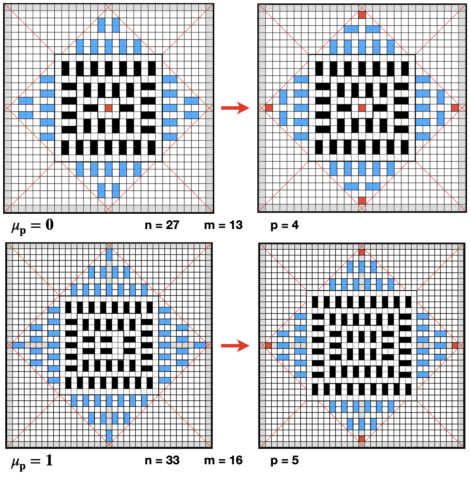
Figure 20: Injection of disorder in Class $11$, case $\mu_{p}=1$. (Left) Some vacant space, with or without lacunar void, can accommodate an additional domino but this anomaly cannot be propagated beyond small values of $n$. (Right) Enlarging the square core from size $f_{11}(m)=m-1$ to size $f_{11}(m)+2=m+1.$ The number of dominos remains unchanged but this transformation releases four lacunar voids on the tips.

Figure 21: Injection of disorder in Class $11$: this transformation yields a potential $\overline{\psi}_{n}=\psi_{n}+2$ of two additional dominos whatever the parity of $p$.
($\uparrow$) $\mu_{p}=0$ – Ridge–flattening on the tip. ($\downarrow$) $\mu_{p}=1$ – Enlarging the core size.

• $\mu_{p}=1$ – Fig. 21 displays a possible change by breaking symmetry but this anomaly cannot be propagated beyond some low value of $n$. Instead, we choose another symmetric transformation by enlarging the square core from size $f_{11}(m)=m-1$ to size $f_{11}(m)+2=m+1$ as follows. From (10) and from (29) the core gets the gain $\xi_{m+1}-\xi_{m-1}=2\,p+2$ but this results in the loss of one row for the wedge resulting from the reduction $h_{11}(m)\rightarrow h_{11}(m)-1$ by turning the top domino into a lacunar void, as well as a deficit of one domino per row resulting from the reduction $b_{11}(m)\rightarrow b_{11}(m)-2$ whence an overall deficit of $(p+1)/2$ dominos per wedge, that is, a deficit of $2\,p+2$ in total which compensates for the above core’s gain. The number of dominos thus remains unchanged but this transformation releases four additional lacunar voids, giving a potential of two additional dominos, whence an ultimate potential capacity of $\psi_{n}+2$.

• $\mu_{p}=0$ – A ridge–flattening will yield four lacunar voids in all, giving a potential capacity of $\psi_{n}+2$.

An illustration of this general transformation, whatever the parity of $p$, is displayed in Fig. 21. This transformation holds for any $p>0$ in Class $11$, whence

$$\forall m\equiv_{3}1,\ p>0,\ n=2\,m+1:\hskip 14.22636pt\overline{\psi}_{n}=\psi_{n}+2$$ (118)

where $\overline{\psi}_{n}$ denotes the extended capacity resulting from this transformation.

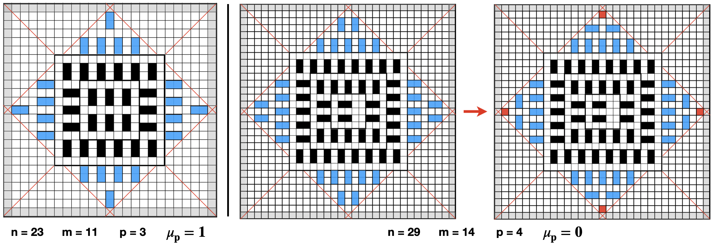
Figure 22: Injection of disorder in Class $12$: this transformation yields a potential $\overline{\psi}_{n}=\psi_{n}+2\,(1-\mu_{p}).$
(Left) $\mu_{p}=1$ – The configuration is optimal. (Right) $\mu_{p}=0$ – Ridge–flattening.

6.1.3 In Class $12$

According to Fig. 22 no change is made for $\mu_{p}=1$ whereas for $\mu_{p}=0$ a ridge–flattening will yield a potential $\overline{\psi}_{n}=\psi_{n}+2$ of two additional dominos. This transformation holds for any $p>0$ in Class $12$, whence

$$\forall m\equiv_{3}2,\ p>0,\ n=2\,m+1:\hskip 14.22636pt\overline{\psi}_{n}=\psi_{n}+2\,(1-\mu_{p})$$ (119)

where $\overline{\psi}_{n}$ denotes the extended capacity resulting from this transformation. For $\mu_{p}=1$ the lower bound $\psi_{n}$ reaches the upper bound $\overline{\psi}_{n}$ therefore, in this case, $\psi_{n}=\overline{\psi}_{n}$ is the exact domino number for a maximal arrangement in $\mathcal{D}_{n}.$

6.2 Injection of Disorder – $n$ even

A first observation of Fig. 8 shows that some lacunar voids emerge as isolated cells from $n>20$. It will even be stated that this emergence actually occurs from $n=20$ in Class $01$. In other words, Region $\mathcal{W}^{\prime\prime}_{0m}$ is empty below this threshold, hereafter denoted $\mathbf{n}_{w^{\prime\prime}}.$

The second observation is again related to the central pattern of the square core: a vacant space, with or without lacunar void, is likely to cause a deficit in the whole. Referring to Fig. 9 such a situation exists for $\mathcal{S}_{2}$ – condition noted briefly $(\mbox{s}_{2})$ – but neither for $\mathcal{S}_{0}$ nor for $\mathcal{S}_{4}.$

Now, for $n\geq\mathbf{n}_{w^{\prime\prime}}$ any deficiency of the core will be compensated by the potential induced by the emergence of lacunar voids. It follows that a non–optimality problem will be induced by the conjunction $(\mbox{s}_{2})\land(n<\mathbf{n}_{w^{\prime\prime}}).$ It can again be released either by enlarging or by shrinking the core size, or by applying a local transformation. One case per class is involved: $n=6$ for Class $00$, $n=20$ for Class $01$, $n=16$ for Class $02$.

6.2.1 In Class $00$

By referring to the relation in (43) connecting $p+1$ and $r_{p+1}$ and to the periodic sequence of expansion of $W^{\prime\prime}_{00}$ in (67) and beyond, we observe for any $p>0$ the emergence of a new lacunar void per wedge at $r_{p+1}=1,$ that is at $p\equiv_{4}0.$ That gives $4\,\lfloor\,p/4\,\rfloor$ voids in all and thus an additional potential of $2\,\lfloor\,p/4\,\rfloor$ dominos, whence

$$\forall m\equiv_{3}0,\ n=2\,m:\hskip 14.22636pt\overline{\psi}_{n}=\psi_{n}+2\,\lfloor\,p/4\,\rfloor$$ (120)

where $\overline{\psi}_{n}$ denotes the resulting extended capacity. The distribution of lacunar voids could already be observed in Fig. 8 and Fig. 15 for Class $00$.

Moreover, it should be pointed out that the critical case mentioned above in this class ($n=6$), while satisfying the condition $(\mbox{s}_{2})\land(n<\mathbf{n}_{w^{\prime\prime}}),$ necessary but not sufficient, remains optimal beyond the unsuccessful transformations of Fig. 23.

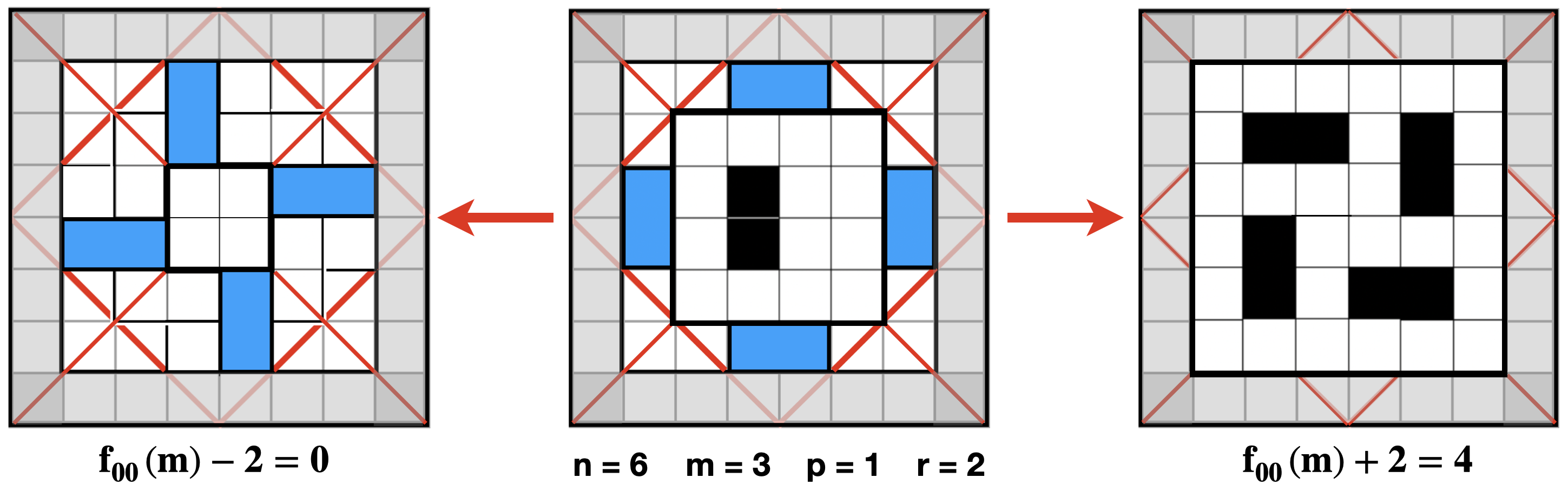
Figure 23: Injection of disorder in Class $00$ for $r_{p+1}=2$. Neither shrinking ($\leftarrow$) the square core to size $f_{00}(m)-2$ nor enlarging it ($\rightarrow$) to size $f_{00}(m)+2$ gives better capacity than the basic configuration for $n=6$ in Fig. 8.

6.2.2 In Class $01$

By referring to the relation in (43) connecting $p$ and $r_{p}$ and to the periodic sequence of expansion of $W^{\prime\prime}_{01}$ in (96), we observe for any $p>0$ the emergence of a new lacunar void at $r_{p}=0.$ However, we also observe that there is a space at $r_{p}=3$ to insert a new lacunar void but, by symmetry, this void remains closed by the baserow of the East wedge. In fact, everything happens as if this void nevertheless had the property of having to be taken into account. This fact finally becomes true, hence at $p+1\equiv_{4}0,$ by applying the slight transformation illustrated in Fig. 24. That gives $4\,\lfloor\,(p+1)/4\,\rfloor$ voids in all and thus an additional potential of $2\,\lfloor\,(p+1)/4\,\rfloor$ dominos, whence

$$\forall m\equiv_{3}1,\ n=2\,m:\hskip 14.22636pt\overline{\psi}_{n}=\psi_{n}+2\,\lfloor\,(p+1)/4\,\rfloor$$ (121)

where $\overline{\psi}_{n}$ denotes the extended capacity resulting from such a transformation. The distribution of lacunar voids could already be observed in Fig. 8 and Fig. 16 for Class $01$.

Note that the previously mentioned critical case in this class ($n=20$) coincide with the threshold $\mathbf{n}_{w^{\prime\prime}}$ of lacunar emergence.

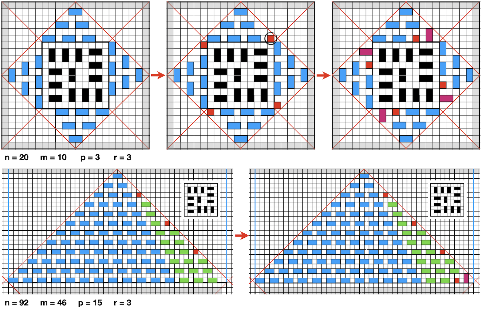
Figure 24: Injection of disorder in Class $01$ – Implicit void in the baserow of the wedge for $r_{p}=3$, taking an explicit form after a slight transformation.

6.2.3 In Class $02$

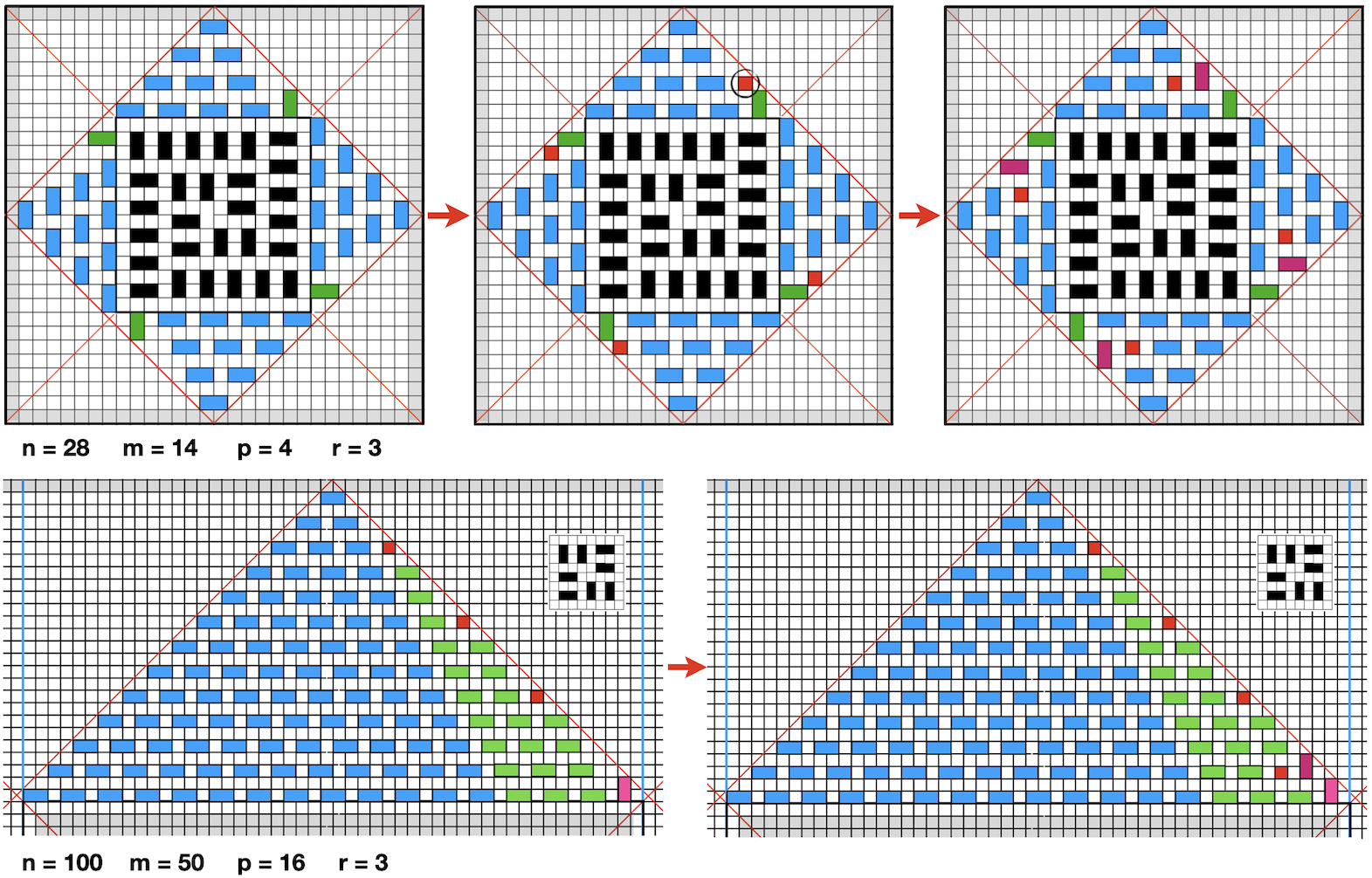
Figure 25: Injection of disorder in Class $02$ for $r_{p-1}=3$ – Implicit void in the penultimate row of the wedge, taking an explicit form after a slight transformation.

This class is the most intricate and several cases should be examined. We refer again to the corresponding relation in (43) connecting $p-1$ and $r_{p-1}$ and to the periodic sequence of expansion of $W^{\prime\prime}_{02}$ in (115). Without loss of generality, suppose first that

$$\forall m\equiv_{3}2,\ n=2\,m:\hskip 14.22636pt\psi_{n}^{+}=\psi_{n}+2\,\lfloor\,(p+2)/4\,\rfloor$$ (122)

where $\psi_{n}^{+}$ denotes the extended capacity that would result from the following counting and transformations.

• $r_{p-1}=3$  — The new lacunar void, emerging in the baserow of the previous step at $r_{p-1}=2$, disappears under the effect of the vertical rotation of the new domino inserted in the new baserow (see Fig. 8 and Fig. 17). In fact, everything happens as if this void nevertheless had the property of having to be taken into account. This fact finally becomes true by applying the slight transformation illustrated in Fig. 25 then the potential capacity $\psi_{n}^{+}$ assumed in (122) remains valid.

  

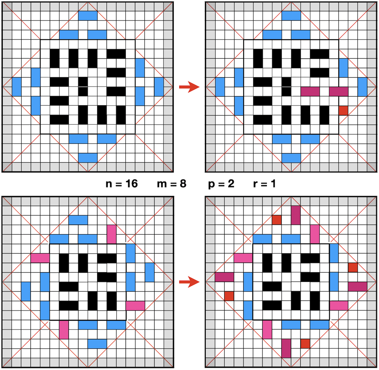
  Figure 26: Injection of disorder in Class $02$ for $r_{p-1}=1$ – ($\uparrow$) Releasing a lacunar void from some vacancy in the core. ($\downarrow$) Shrinking the square core from size $f_{02}(m)=m$ to size $f_{02}(m)-2$ with reduction $\xi_{m-2}-\xi_{m}=-\,(2\,p+1)=-5$ for this case; overall gain of $2p=4$ for the wedges; overall loss of one domino altogether; overall gain of four lacunar voids giving a potential of two additional dominos. Initial configuration with $\psi_{n}=25$, final configuration with $\psi_{n}-1=24$, potential capacity $\overline{\psi}_{n}=26$.

  

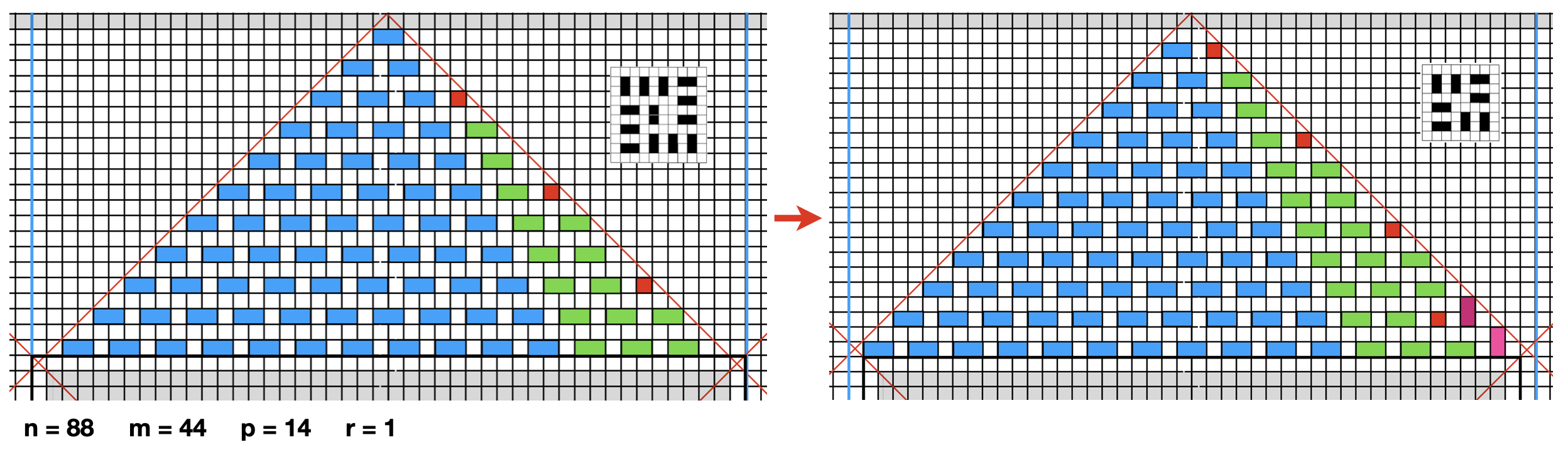
  Figure 27: Injection of disorder in Class $02$ for $r_{p-1}=1$ – Shrinking the square core. After shrinking, the resulting configuration of Region $\mathcal{W}^{\prime\prime}_{02}$ becomes a copy of itself after the same slight transformation for $r_{p-1}=3$ in Fig. 25.

• $r_{p-1}=1$  — In the center of the core, we can observe some vacancy which is likely to allow the emergence of voids as shown in Fig. 26. We therefore choose a symmetric transformation by shrinking the square core from size $f_{02}(m)=m$ (from (44)) to size $f_{02}(m)-2.$ Then $\xi_{m-2}-\xi_{m}=-\,(2\,p+1)$ from (103) but this results in the gain $h_{02}(m)\rightarrow h_{02}(m)+1$ of one row for the wedge as well as the expansion $b_{02}(m)\rightarrow b_{02}(m)+2$ of two cells for the new baserow. As a consequence, the block of Region $\mathcal{W}^{\prime}_{02}$ is shifted both downward and leftward while remaining adjacent to the shrunk core whereas capacity $W^{\prime}_{02}$ remains unchanged.

  On the other hand, it follows that the configuration of Region $\mathcal{W}^{\prime\prime}_{02}$ turns into a copy of that at $r_{p-1}=3$ within the $q_{p-1}$–cycle (at constant $q_{p-1}$). Thus by achieving the suitable assessments from (115) we obtain the gain

  $$W^{\prime\prime}_{02}(p+2)-W^{\prime\prime}_{02}(p)=(W^{\prime\prime}_{02}(p+2)-W^{\prime\prime}_{02}(p+1))+(W^{\prime\prime}_{02}(p+1)-W^{\prime\prime}_{02}(p))$$

  namely

  $$(q_{p-1}-1+\delta_{3})+(q_{p-1}-1+\delta_{2})$$

  and since $\delta_{3}=2$ and $\delta_{2}=1$ from (110) we obtain the gain $2\,q_{p-1}+1=p/2$ per wedge and therefore an overall gain of $2\,p$ for the four wedges. Finally the overall gain becomes $-\,(2\,p+1)+2\,p=-1,$ i.e. an overall loss of one domino.

Regarding Region $\mathcal{W}^{\prime\prime}_{02}$ it is worth comparing the last configuration in Figs. 26 & 25 (resp. for ($n=16,r_{p-1}=1$) & ($n=28,r_{p-1}=3$)) and the last configuration in Figs. 27 & 25 (resp. for ($n=88,r_{p-1}=1$) & ($n=100,r_{p-1}=3$)).

Finally, the extended capacity $\psi_{n}^{+}$ in (122) holds almost everywhere, except for the loss of one domino for $r_{p-1}=1$ whence the final expression

$$\forall m\equiv_{3}2,\ n=2\,m:\hskip 14.22636pt\overline{\psi}_{n}=\psi_{n}+2\,\lfloor\,(p+2)/4\,\rfloor-\lambda_{r_{p-1}}$$ (123)

where $\lambda_{r_{p-1}}=1$ for $r_{p-1}=1$ and $\lambda_{r_{p-1}}=0$ otherwise and where $\overline{\psi}_{n}$ denotes the resulting extended capacity in Class $02$.

7 Discussion and Future Issues

The subject herein was to find a maximal arrangement of dominos in the diamond $\mathcal{D}_{n}$ of size $n$. The words “domino” and “diamond” are understood according to their exact meaning defined in Sect. 2. This construction was carried out in two stages. First, a deterministic arrangement was proposed which led to a sub–optimal solution $\psi_{n}$ as the lower bound. Second, some disorder has been injected, leading to an upper bound $\overline{\psi}_{n}$ reachable or not. Despite our inability to achieve the optimal $\psi_{n}^{\ast}$ for any $n$, we have nevertheless made a significant advance. The main results are presented hereafter.

Linear evolution of the ratio $\overline{\psi}_{n}/n$.

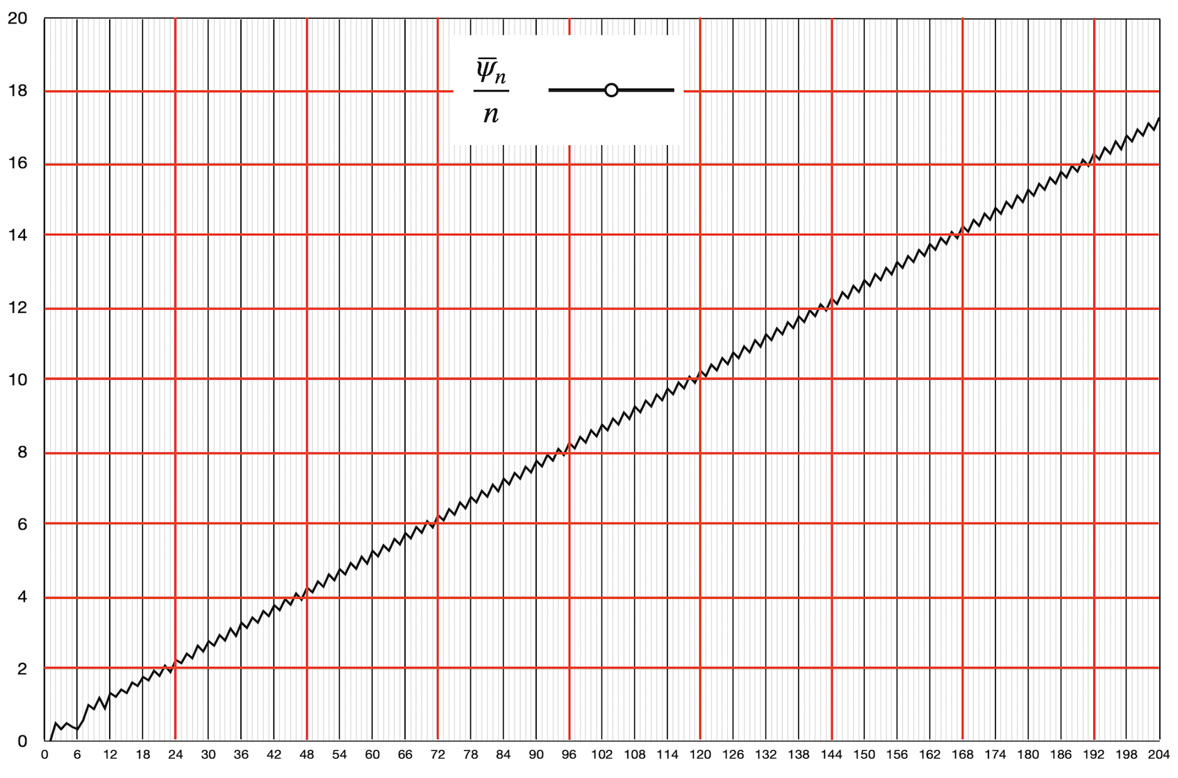
Figure 28: Linear evolution on average of the ratio $\overline{\psi}_{n}/n$ vs $n$ after a chaotic behavior for small values of $n$. The graph is a discrete dust of points in $\mathbb{N}\times\mathbb{Q}$ with jump discontinuities, represented as a sawtooth continuous line.

It is not a breakthrough to observe in Fig. 28 that the slope of ${\overline{\psi}_{n}}/{n}$ (vs. $n$) is linear on average after a chaotic behavior for small values of $n$. At this scale, we are allowed to disregard the negligible deviation $\overline{\psi}_{n}-\psi_{n}$ as it will be examined thereafter. As a first approximation, the linearity is evidenced for the odd $n$ in (27, 34, 41) by the linear rate of change $\psi_{n}-\psi_{n-6}$ following a $p\rightarrow p+1$ cycle within any Class $1m$.

For the even $n$, in spite of the fluctuations observed in Tabs. 1–3 a linear rate of change $\psi_{n}-\psi_{n-24}$ is nevertheless observed in (78, 97, 116) at a larger scale following a $p\rightarrow p+4$ cycle within any Class $0m$.

The graph of ${\overline{\psi}_{n}}/{n}$ is a sawtooth curve (the “curve” should be seen here as a discrete dust of points in $\mathbb{N}\times\mathbb{Q})$ with jump discontinuities. This phenomenon is explained by the “von Neumann $\leftrightarrow$ Aztec” expansion $|\mathcal{D}_{n}|-|\mathcal{D}_{n-1}|$ in (4) where the diamond grows significantly only one time out of two.

Evolution of the global occupancy towards the optimum.

Fig. 29 shows the evolution with $n$ of the global occupancy $|\mathcal{D}_{n}|/{\overline{\psi}_{n}}$ – as defined in Subsect. 2.2 – which decreases asymptotically towards its optimal limit. The graph is again a sawtooth curve (as discrete dust of points in $\mathbb{N}\times\mathbb{Q})$ with jump discontinuities. Again we are allowed to disregard the deviation $\overline{\psi}_{n}-\psi_{n}$ negligible at this scale. We examine the following two cases

• in Class $10$ — From the cardinality of $\mathcal{D}_{n}$ in (2) and the direct expression of $\psi_{n}$ in (26) it comes

  $$\lim\limits_{n\rightarrow+\infty}\frac{\mid\mathcal{D}_{n}\mid}{\psi_{n}}=\lim\limits_{n\rightarrow+\infty}\frac{(n^{2}+4n+5)/2}{(n^{2}-1)/12}=\lim\limits_{n\rightarrow+\infty}6\cdot(1+\frac{4}{n}\,)$$

  and the global occupancy tends to the optimum – the blue asymptote – as $n$ tends to infinity. The same result is obtained in Class $11$ from (33) and in Class $12$ from (40).

• in Class $00$ — For lack of a simple, direct expression of $\psi_{n}$ for this class, we assume $p>4$ and refer to the linear rate of change $\psi_{n}-\psi_{n-24}$ in (78) following a $p\rightarrow p+4$ cycle. Now, from the cardinality of $\mathcal{D}_{n}$ in (3) it comes

  $$\mid\mathcal{D}_{n-24}\mid=((n-24)^{2}+6\,(n-24)+8)/2=\,\mid\mathcal{D}_{n}\mid-\ 24\,(n-9)$$

  whereas $\psi_{n-24}=\psi_{n}-4\,(n-11)$ from (78). Therefore, if the ratio $|\mathcal{D}_{n}|/\psi_{n}$ admits a limit when $n$ goes to infinity, then it must follow a Cauchy sequence. Now

  $$\frac{\mid\mathcal{D}_{n}\mid}{\psi_{n}}\sim\frac{\mid\mathcal{D}_{n-24}\mid}{\psi_{n-24}}=\frac{\mid\mathcal{D}_{n}\mid-\,24\,(n-9)}{\psi_{n}-4\,(n-11)}$$

  whence

  $$\mid\mathcal{D}_{n}\mid(\psi_{n}-4\,(n-11))\sim\psi_{n}\,(\mid\mathcal{D}_{n}\mid-\,24\,(n-9))$$

  $$\Rightarrow 4\,(n-11)\mid\mathcal{D}_{n}\mid\ \sim 24\,(n-9)\,\psi_{n}$$

  and finally

  $$\lim\limits_{n\rightarrow+\infty}\frac{\mid\mathcal{D}_{n}\mid}{\psi_{n}}=\lim\limits_{n\rightarrow+\infty}6\cdot\frac{n-9}{n-11}=\lim\limits_{n\rightarrow+\infty}6\cdot(1+\frac{2}{n}\,)$$

  and the global occupancy tends to the optimum. The same result is obtained in Class $01$ from (97) and in Class $02$ from (116).

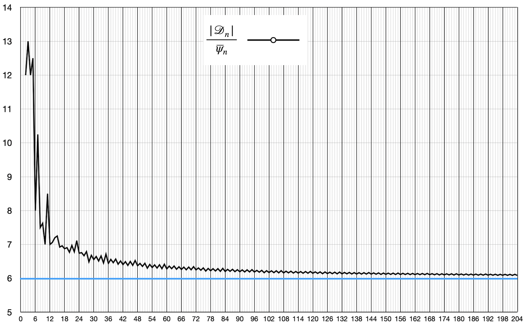
Figure 29: Beyond a chaotic behavior for small $n$, evolution of the global occupancy $|\mathcal{D}_{n}|/{\overline{\psi}_{n}}$ vs $n$ towards the optimum – the blue line. The graph is a sawtooth discrete dust of points in $\mathbb{N}\times\mathbb{Q}$ with jump discontinuities.

Absolute and relative deviations between lower and upper bounds.

We now focus on the deviation $\Delta\psi_{n}=\overline{\psi}_{n}-\psi_{n}\geq 0$ between the suboptimal lower bound $\psi_{n}$ and the upper bound $\overline{\psi}_{n}$ reachable or not, produced after injection of disorder. The two following cases depend on the parity of $n$.

• $n$ odd — By grouping all the cases resulting from (117–119) it comes

  $$\overline{\psi}_{n}-\psi_{n}=\left\{\begin{array}[]{ll}0&\mbox{ in {Class} $12$ \ if $p$ odd }\\ 2&\mbox{ otherwise }\end{array}\right.$$

  namely $\overline{\psi}_{n}-\psi_{n}=2$ in general, except in one case where the exact value is obtained. Moreover, from the conditions on $p$ in (117–119) the exact value is also checked for small $p<2$ ($n<12$) except for $n=9$. The relative deviation $\Delta\psi_{n}/\psi_{n}$ in the general case, is only relevant beyond the chaotic domain highlighted in Fig. 29, namely for $n\geq 24$ and can be expressed as follows. For $n$ large, we can consider from (26, 33, 40) that $\psi_{n}\sim n^{2}/12$ and $\Delta\psi_{n}/\psi_{n}\sim 24/n^{2}$ thereof. There is a near coincidence of the lower and upper curves.

• $n$ even — Without going into details, we can estimate from (120, 121, 123) that the absolute deviation behaves like

  $$\overline{\psi}_{n}-\psi_{n}\approx 2\,\Bigl{\lfloor}\,\frac{p+m\bmod 3}{4}\,\Bigr{\rfloor}$$

  approximately. As a result, we get a collection of exact values of $\psi_{n}$ for almost small $p<4$ ($n<24$). For the relative deviation with large $n$, we can approach $\psi_{n}$ as above with $\psi_{n}\sim n^{2}/12$ and the absolute deviation with $\Delta\psi_{n}\sim p/2$ to get $\Delta\psi_{n}/\psi_{n}\sim 1/n$ thereof. For instance, for $n=200$ we get $\Delta\psi_{n}/\psi_{n}\approx$ 5 ‰.

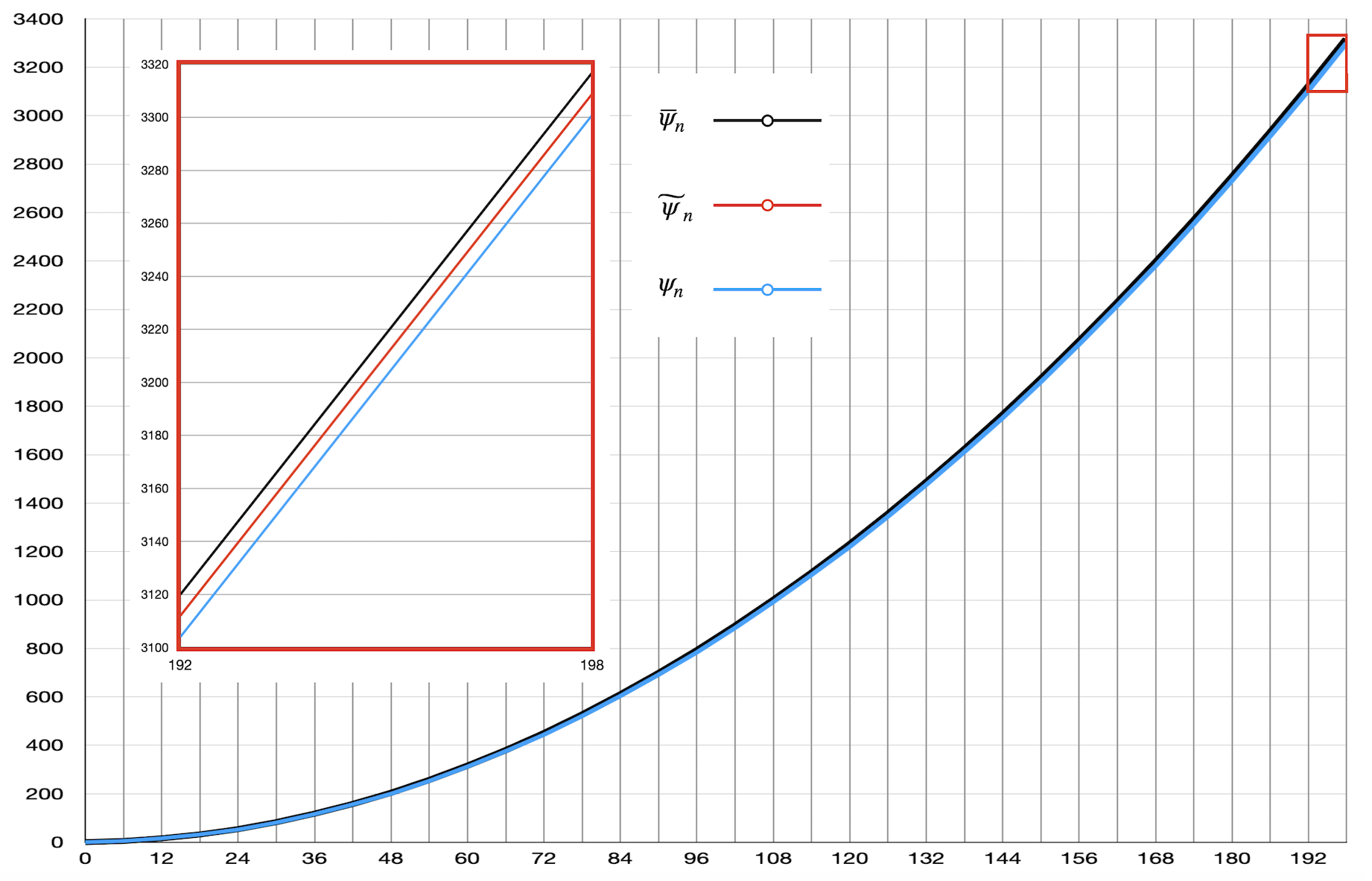
Figure 30: Evolution of the population of dominos in diamond $\mathcal{D}_{n}$ – Class $00$. Lower bound $\psi_{n}$, upper bound $\overline{\psi}_{n}$ and median estimation $\widetilde{\psi}_{n}=(\psi_{n}+\overline{\psi}_{n})/2$. Each graph of $(\psi_{n},\overline{\psi}_{n})$ vs $n$ is now a discrete dust of points in $\mathbb{N}\times\mathbb{N}$ located on a smooth parabola. Zoom on the small red window in the interval $n\in[192,198]$.

Fig. 30 shows the evolution of the population in diamond $\mathcal{D}_{n}$ – Class $00$ – and the deviation between lower bound $\psi_{n}$ and upper bound $\overline{\psi}_{n}$. Each graph is now a discrete dust of points in $\mathbb{N}\times\mathbb{N}$ located on a smooth parabola and this would also be the case for each of the six classes $nm$. The divergence $\overline{\psi}_{n}-\psi_{n}$ within the small red window is highlighted.

A question arises whether the upper bound is excessive or not. The expression for $\overline{\psi}_{n}$ in Sect. 6 was based on this harsh assumption that “in a disordered system two lacunar voids are likely to join together, that yields a potential of one additional domino” namely, only a potential. A median estimate $\widetilde{\psi}_{n}=(\psi_{n}+\overline{\psi}_{n})/2$ – as highlighted in Fig. 30 – would perhaps be more appropriate by estimating a fifty percent chance of marrying two monominos (the lacunar voids) to give birth to a domino.

Conclusion.

In this study, we can deplore the weakness of obtaining only an estimate $\widetilde{\psi}_{n}$ in general and of obtaining the exact maximum only in a few cases. This discrepancy is indeed an open problem. It could be partially filled by better theory as well as by the use of simulation and, if possible, improved by high performance computing. This technical study will serve as a companion paper to support further comparative study with the simulation model already tackled in [4]. These new results will be examined elsewhere. Obtaining new occurrences $\psi_{n}^{(s)}=\overline{\psi}_{n}$ – where $\psi_{n}^{(s)}$ is the result of a simulation for a given $n$ – would indeed be likely to expand the collection of exact values. Be that as it may, this search for a maximum could at least remain the subject of a mathematical game, or of entertainment, or of a brain training challenge.

Appendix – Domino Enumeration

This appendix brings together all the expressions and formulas that have been developed throughout this study and gives a numerical evaluation of them on a sample of 200 values of $n$.

The first two tables (Tabs. 4–5) give an overview of the capacity of the regions in $\mathcal{D}_{n}$ according to the construction rule, and leading to the different expressions of $\psi_{n}$.

The following eight tables (Tabs. 6–13) list the various counts of the maximum layouts of dominos in the square and the diamond.

The first two relate to the square $\mathcal{S}_{n}$ of odd dimension (Table 6) and then of even dimension (Table 7).

The next six relate to the diamond $\mathcal{D}_{n}$ and are divided into two groups of three, first of odd dimension (Tabs. 8–10) then of even dimension (Tabs. 11–13). The penultimate column lists the theoretical estimate $\psi_{n}$ and the last column lists the upper bound $\overline{\psi}_{n}$.

For the sake of clarity, each of the tables is preceded by the list of its various components.

Table 4: Capacity $\psi_{n}$ in $\mathcal{D}_{n}$ according to the three classes $\texttt{C}1m$ — $n=2m+1$. Detail of the different regions (core and wedges). The $\psi_{n}$ is expressed in various forms, either direct or following a recurrence relation.

Table 5: Part I — Capacity $\psi_{n}$ in $\mathcal{D}_{n}$ according to the three classes $\texttt{C}0m$ — $n=2m$. Detail of the different regions (core and wedges). In the table, cells with a given color for the first and second subwedges denote a same wedge–pattern in the diamond (compare Figs. 15–17).

Table 5: Part II — Overall capacity $\psi_{n}$ in $\mathcal{D}_{n}$ according to the three classes $\texttt{C}0m$ — $n=2m$. The $\psi_{n}$ is expressed in various forms, either direct or following a recurrence relation. A color highlights similar expressions for the direct form.

Table 6: Domino enumeration in the Square — $p\,\in\,\mathbb{N}\,;\hskip 5.69054ptn\,\mbox{ odd }\,;$

$\xi_{1}=0,\,\xi_{3}=2,\,\xi_{5}=6\hskip 8.53581pt\mbox{and}\hskip 8.53581pt\xi_{n}=\xi_{n-6}+2(n-2)\,;$

$\texttt{Class}\ (\dot{10}):\ m\,=3\,p\,;\hskip 5.69054ptn\,=2\,m+1\,;\hskip 8.53581pt\xi_{n}=(n-1)(n+3)/\,6\,;$

$\texttt{Class}\ (\dot{11}):\ m\,=3p+1\,;\hskip 5.69054ptn\,=2\,m+1\,;\hskip 8.53581pt\xi_{n}=(n-1)(n+3)/\,6\,;$

$\texttt{Class}\ (\dot{12}):\ m\,=3p+2\,;\hskip 5.69054ptn\,=2\,m+1\,;\hskip 8.53581pt\xi_{n}=(n+1)^{2}/\,6\,;$

	Class  ($\dot{10})$			Class  ($\dot{11})$			Class  ($\dot{12})$
$\ \ p\ \$	$\ \ m\ \$	$\ \ n\ \$	$\ \ \xi_{n}$	$\ \ m\ \$	$\ \ n\ \$	$\ \ \xi_{n}$	$\ \ m\ \$	$\ \ n\ \$	$\ \ \xi_{n}$
0	0	1	0	1	3	2	2	5	6
1	3	7	10	4	9	16	5	11	24
2	6	13	32	7	15	42	8	17	54
3	9	19	66	10	21	80	11	23	96
4	12	25	112	13	27	130	14	29	150
5	15	31	170	16	33	192	17	35	216
6	18	37	240	19	39	266	20	41	294
7	21	43	322	22	45	352	23	47	384
8	24	49	416	25	51	450	26	53	486
9	27	55	522	28	57	560	29	59	600
10	30	61	640	31	63	682	32	65	726
11	33	67	770	34	69	816	35	71	864
12	36	73	912	37	75	962	38	77	1014
13	39	79	1066	40	81	1120	41	83	1176
14	42	85	1232	43	87	1290	44	89	1350
15	45	91	1410	46	93	1472	47	95	1536
16	48	97	1600	49	99	1666	50	101	1734
17	51	103	1802	52	105	1872	53	107	1944

Table 7: Domino enumeration in the Square — $p\,\in\,\mathbb{N}\,;\hskip 5.69054ptn\,\mbox{ even }\,;$

$\xi_{0}=0,\,\xi_{2}=1,\,\xi_{4}=4\hskip 8.53581pt\mbox{and}\hskip 8.53581pt\xi_{n}=\xi_{n-6}+2(n-2)\,;$

$\texttt{Class}\ (\dot{00}):\ m\,=3\,p\,;\hskip 5.69054ptn\,=2\,m\,;\hskip 8.53581pt\xi_{n}=n(n+2)/\,6\,;$

$\texttt{Class}\ (\dot{01}):\ m\,=3p+1\,;\hskip 5.69054ptn\,=2\,m\,;\hskip 8.53581pt\xi_{n}=(n\,(n+2)-2)/\,6\,;$

$\texttt{Class}\ (\dot{02}):\ m\,=3p+2\,;\hskip 5.69054ptn\,=2\,m\,;\hskip 8.53581pt\xi_{n}=n(n+2)/\,6\,;$

	Class  ($\dot{00})$			Class  ($\dot{01})$			Class  ($\dot{02})$
$\ \ p\ \$	$\ \ m\ \$	$\ \ n\ \$	$\ \ \xi_{n}$	$\ \ m\ \$	$\ \ n\ \$	$\ \ \xi_{n}$	$\ \ m\ \$	$\ \ n\ \$	$\ \ \xi_{n}$
0	0	0	0	1	2	1	2	4	4
1	3	6	8	4	8	13	5	10	20
2	6	12	28	7	14	37	8	16	48
3	9	18	60	10	20	73	11	22	88
4	12	24	104	13	26	121	14	28	140
5	15	30	160	16	32	181	17	34	204
6	18	36	228	19	38	253	20	40	280
7	21	42	308	22	44	337	23	46	368
8	24	48	400	25	50	433	26	52	468
9	27	54	504	28	56	541	29	58	580
10	30	60	620	31	62	661	32	64	704
11	33	66	748	34	68	793	35	70	840
12	36	72	888	37	74	937	38	76	988
13	39	78	1040	40	80	1093	41	82	1148
14	42	84	1204	43	86	1261	44	88	1320
15	45	90	1380	46	92	1441	47	94	1504
16	48	96	1568	49	98	1633	50	100	1700
17	51	102	1768	52	104	1837	53	106	1908

Table 8: Domino enumeration in the Diamond – Class $10$.
— $p\,\in\,\mathbb{N}\,;\hskip 5.69054ptm\,=3\,p\,;\hskip 5.69054ptn\,=2\,m+1\,;$

$f_{10}(m)=m-1-\mu_{p}\,;\hskip 8.53581pt\psi_{n}=\xi_{f_{10}(m)}+4\,W_{10}(p)\,;$

$W_{10}(p)=(p+\mu_{p})\,(3\,p+2-\mu_{p})/8\,;\hskip 8.53581pt\xi_{f_{10}(m)}:$ refer to Tab. 6 ;

$\psi_{1}=0\,;\hskip 8.53581pt\psi_{n}=\psi_{n-6}+(n-3)\hskip 11.38109pt(p>0)\,;$

$\psi_{n}=p\,(3p+1)=(n-1)(n+1)/12\,;$

$\overline{\psi}_{n}=\psi_{n}+2\hskip 11.38109pt(p>1)$

$\ \ n\ \$	$\ \ m\ \$	$\ \ p\ \$	$\ \mu_{p}\$	$f_{10}(m)$	$\xi_{f_{10}(m)}$	$W_{10}(p)$	$\ \ \psi_{n}$	$\ \ \overline{\psi}_{n}$
1	0	0	0	–	–	0	0	0
7	3	1	1	1	0	1	4	4
13	6	2	0	5	6	2	14	16
19	9	3	1	7	10	5	30	32
25	12	4	0	11	24	7	52	54
31	15	5	1	13	32	12	80	82
37	18	6	0	17	54	15	114	116
43	21	7	1	19	66	22	154	156
49	24	8	0	23	96	26	200	202
55	27	9	1	25	112	35	252	254
61	30	10	0	29	150	40	310	312
67	33	11	1	31	170	51	374	376
73	36	12	0	35	216	57	444	446
79	39	13	1	37	240	70	520	522
85	42	14	0	41	294	77	602	604
91	45	15	1	43	322	92	690	692
97	48	16	0	47	384	100	784	786
103	51	17	1	49	416	117	884	886
109	54	18	0	53	486	126	990	992
115	57	19	1	55	522	145	1102	1104
121	60	20	0	59	600	155	1220	1222
127	63	21	1	61	640	176	1344	1346
133	66	22	0	65	726	187	1474	1476
139	69	23	1	67	770	210	1610	1612
145	72	24	0	71	864	222	1752	1754
151	75	25	1	73	912	247	1900	1902
157	78	26	0	77	1014	260	2054	2056
163	81	27	1	79	1066	287	2214	2216
169	84	28	0	83	1176	301	2380	2382
175	87	29	1	85	1232	330	2552	2554
181	90	30	0	89	1350	345	2730	2732
187	93	31	1	91	1410	376	2914	2916
193	96	32	0	95	1536	392	3104	3106
199	99	33	1	97	1600	425	3300	3302

Table 9: Domino enumeration in the Diamond – Class $11$.
— $p\,\in\,\mathbb{N}\,;\hskip 5.69054ptm\,=3\,p+1\,;\hskip 5.69054ptn\,=2\,m+1\,;$

$f_{11}(m)=m-\mu_{p}\,;\hskip 8.53581pt\psi_{n}=\xi_{f_{11}(m)}+4\,W_{11}(p)\,;$

$W_{11}(p)=(p+\mu_{p})\,(3\,p+2-\mu_{p})/8\,;\hskip 8.53581pt\xi_{f_{11}(m)}:$ refer to Tab. 6 ;

$\psi_{3}=1\,;\hskip 8.53581pt\psi_{n}=\psi_{n-6}+(n-3)\hskip 11.38109pt(p>1)\,;$

$\psi_{n}=3\,p\,(p+1)=(n-3)(n+3)/12\,;\hskip 11.38109pt(p>0)$

$\overline{\psi}_{n}=\psi_{n}+2\hskip 11.38109pt(p>0)$

$\ \ n\ \$	$\ \ m\ \$	$\ \ p\ \$	$\ \mu_{p}\$	$f_{11}(m)$	$\xi_{f_{11}(m)}$	$W_{11}(p)$	$\ \ \psi_{n}$	$\ \ \overline{\psi}_{n}$
3	1	0	0	1	0	0	1	1
9	4	1	1	3	2	1	6	8
15	7	2	0	7	10	2	18	20
21	10	3	1	9	16	5	36	38
27	13	4	0	13	32	7	60	62
33	16	5	1	15	42	12	90	92
39	19	6	0	19	66	15	126	128
45	22	7	1	21	80	22	168	170
51	25	8	0	25	112	26	216	218
57	28	9	1	27	130	35	270	272
63	31	10	0	31	170	40	330	332
69	34	11	1	33	192	51	396	398
75	37	12	0	37	240	57	468	470
81	40	13	1	39	266	70	546	548
87	43	14	0	43	322	77	630	632
93	46	15	1	45	352	92	720	722
99	49	16	0	49	416	100	816	818
105	52	17	1	51	450	117	918	920
111	55	18	0	55	522	126	1026	1028
117	58	19	1	57	560	145	1140	1142
123	61	20	0	61	640	155	1260	1262
129	64	21	1	63	682	176	1386	1388
135	67	22	0	67	770	187	1518	1520
141	70	23	1	69	816	210	1656	1658
147	73	24	0	73	912	222	1800	1802
153	76	25	1	75	962	247	1950	1952
159	79	26	0	79	1066	260	2106	2108
165	82	27	1	81	1120	287	2268	2270
171	85	28	0	85	1232	301	2436	2438
177	88	29	1	87	1290	330	2610	2612
183	91	30	0	91	1410	345	2790	2792
189	94	31	1	93	1472	376	2976	2978
195	97	32	0	97	1600	392	3168	3170
201	100	33	1	99	1666	425	3366	3368

Table 10: Domino enumeration in the Diamond – Class $12$.
— $p\,\in\,\mathbb{N}\,;\hskip 5.69054ptm\,=3\,p+2\,;\hskip 5.69054ptn\,=2\,m+1\,;$

$f_{12}(m)=m+1-\mu_{p}\,;\hskip 8.53581pt\psi_{n}=\xi_{f_{12}(m)}+4\,W_{12}(p)\,;$

$W_{12}(p)=(p+\mu_{p})\,(3\,p+2-\mu_{p})/8\,;\hskip 8.53581pt\xi_{f_{12}(m)}:$ refer to Tab. 6 ;

$\psi_{5}=2\,;\hskip 8.53581pt\psi_{n}=\psi_{n-6}+(n-3)\hskip 11.38109pt(p>0)\,;$

$\psi_{n}=(3\,p+2)\,(p+1)=(n-1)(n+1)/12\,;$

$\overline{\psi}_{n}=\psi_{n}+2\,(1-\mu_{p})\hskip 11.38109pt(p>0)$

$\ \ n\ \$	$\ \ m\ \$	$\ \ p\ \$	$\ \mu_{p}\$	$f_{12}(m)$	$\xi_{f_{12}(m)}$	$W_{12}(p)$	$\ \ \psi_{n}$	$\ \ \overline{\psi}_{n}$
5	2	0	0	3	2	0	2	2
11	5	1	1	5	6	1	10	10
17	8	2	0	9	16	2	24	26
23	11	3	1	11	24	5	44	44
29	14	4	0	15	42	7	70	72
35	17	5	1	17	54	12	102	102
41	20	6	0	21	80	15	140	142
47	23	7	1	23	96	22	184	184
53	26	8	0	27	130	26	234	236
59	29	9	1	29	150	35	290	290
65	32	10	0	33	192	40	352	354
71	35	11	1	35	216	51	420	420
77	38	12	0	39	266	57	494	496
83	41	13	1	41	294	70	574	574
89	44	14	0	45	352	77	660	662
95	47	15	1	47	384	92	752	752
101	50	16	0	51	450	100	850	852
107	53	17	1	53	486	117	954	954
113	56	18	0	57	560	126	1064	1066
119	59	19	1	59	600	145	1180	1180
125	62	20	0	63	682	155	1302	1304
131	65	21	1	65	726	176	1430	1430
137	68	22	0	69	816	187	1564	1566
143	71	23	1	71	864	210	1704	1704
149	74	24	0	75	962	222	1850	1852
155	77	25	1	77	1014	247	2002	2002
161	80	26	0	81	1120	260	2160	2162
167	83	27	1	83	1176	287	2324	2324
173	86	28	0	87	1290	301	2494	2496
179	89	29	1	89	1350	330	2670	2670
185	92	30	0	93	1472	345	2852	2854
191	95	31	1	95	1536	376	3040	3040
197	98	32	0	99	1666	392	3234	3236
203	101	33	1	101	1734	425	3434	3434

Table 11: Domino enumeration in the Diamond – Class $00$.
— $p\,\in\,\mathbb{N}\,;\hskip 5.69054ptm\,=3\,p\,;\hskip 5.69054ptn\,=2\,m\,;$

$p+1=4\,q_{p+1}+r_{p+1}\hskip 5.69054pt(0\leq r_{p+1}<4)\,;\hskip 22.76219ptf_{00}(m)=m+1-r_{p+1}\,;$

$W^{\prime}_{00}(p)=(p-q_{p+1})\,(p-q_{p+1}+1)/2\,;\hskip 22.76219pt\xi_{f_{00}(m)}:$ refer to Tab. 7 ;

$W^{\prime\prime}_{00}(p)=\overline{b^{\prime\prime}}_{00}(m)\cdot((p-q_{p+1}-3)+(p-q_{p+1}-3\cdot\overline{b^{\prime\prime}}_{00}(m))\,/2\,;$

$\overline{b^{\prime\prime}}_{00}(m)=(q_{p+1}-1)+\delta_{r_{p+1}}\hskip 8.53581pt\mbox{with}\hskip 8.53581pt\delta_{r_{p+1}}=\Bigl{\lfloor}r_{p+1}/3\Bigr{\rceil};$

$\psi_{n}=\xi_{f_{00}(m)}+4\,(W^{\prime}_{00}(p)+W^{\prime\prime}_{00}(p))\,;\hskip 8.53581pt\psi_{0}=0\,;\hskip 2.84526pt\psi_{n}=\psi_{n-24}\ +\ 4\ (n-11)\hskip 5.69054pt(p\geq 4)\,;$

$\overline{\psi}_{n}=\psi_{n}+2\,\lfloor\,p/4\,\rfloor$

$\ n\$	$\ m\$	$\ p\$	$r_{p+1}\$	$f_{00}(m)$	$\xi_{f_{00}(m)}$	$W^{\prime}_{00}(p)$	$W^{\prime\prime}_{00}(p)$	$\ \psi_{n}$	$\ \overline{\psi}_{n}$
0	0	0	1	0	0	0	0	0	0
6	3	1	2	2	1	1	0	5	5
12	6	2	3	4	4	3	0	16	16
18	9	3	0	10	20	3	0	32	32
24	12	4	1	12	28	6	0	52	54
30	15	5	2	14	37	10	1	81	83
36	18	6	3	16	48	15	2	116	118
42	21	7	0	22	88	15	2	156	158
48	24	8	1	24	104	21	3	200	204
54	27	9	2	26	121	28	5	253	257
60	30	10	3	28	140	36	7	312	316
66	33	11	0	34	204	36	7	376	380
72	36	12	1	36	228	45	9	444	450
78	39	13	2	38	253	55	12	521	527
84	42	14	3	40	280	66	15	604	610
90	45	15	0	46	368	66	15	692	698
96	48	16	1	48	400	78	18	784	792
102	51	17	2	50	433	91	22	885	893
108	54	18	3	52	468	105	26	992	1000
114	57	19	0	58	580	105	26	1104	1112
120	60	20	1	60	620	120	30	1220	1230
126	63	21	2	62	661	136	35	1345	1355
132	66	22	3	64	704	153	40	1476	1486
138	69	23	0	70	840	153	40	1612	1622
144	72	24	1	72	888	171	45	1752	1764
150	75	25	2	74	937	190	51	1901	1913
156	78	26	3	76	988	210	57	2056	2068
162	81	27	0	82	1148	210	57	2216	2228
168	84	28	1	84	1204	231	63	2380	2394
174	87	29	2	86	1261	253	70	2553	2567
180	90	30	3	88	1320	276	77	2732	2746
186	93	31	0	94	1504	276	77	2916	2930
192	96	32	1	96	1568	300	84	3104	3120
198	99	33	2	98	1633	325	92	3301	3317

Table 12: Domino enumeration in the Diamond – Class $01$.
— $p\,\in\,\mathbb{N}\,;\hskip 5.69054ptm\,=3\,p+1\,;\hskip 5.69054ptn\,=2\,m\,;$

$p=4\,q_{p}+r_{p}\hskip 5.69054pt(0\leq r_{p}<4)\,;\hskip 56.9055ptf_{01}(m)=m+1-r_{p}\,;$

$W^{\prime}_{01}(p)=(p-q_{p})\,(p-q_{p}+1)/2\,;\hskip 28.45274pt\xi_{f_{01}(m)}$ refer to Tab. 7 ;

$W^{\prime\prime}_{01}(p)=\overline{b^{\prime\prime}}_{01}(m)\cdot((p-q_{p}-3)+(p-q_{p}-3\cdot\overline{b^{\prime\prime}}_{01}(m))\,/2\,;$

$\overline{b^{\prime\prime}}_{01}(m)=(q_{p}-1)+\delta_{r_{p}}\hskip 8.53581pt\mbox{with}\hskip 8.53581pt\delta_{r_{p}}=\Bigl{\lfloor}(r_{p}+1)/3\Bigr{\rceil};$

$\psi_{n}=\xi_{f_{01}(m)}+4\,(W^{\prime}_{01}(p)+W^{\prime\prime}_{01}(p))\,;\hskip 8.53581pt\psi_{2}=1\,;\hskip 2.84526pt\psi_{n}=\psi_{n-24}\ +\ 4\ (n-11)\hskip 5.69054pt(p\geq 4)\,;$

$\overline{\psi}_{n}=\psi_{n}+2\,\lfloor(p+1)/4\rfloor$

$\ n\$	$\ m\$	$\ p\$	$r_{p}\$	$f_{01}(m)$	$\xi_{f_{01}(m)}$	$W^{\prime}_{01}(p)$	$W^{\prime\prime}_{01}(p)$	$\ \psi_{n}$	$\ \overline{\psi}_{n}$
2	1	0	0	2	1	0	0	1	1
8	4	1	1	4	4	1	0	8	8
14	7	2	2	6	8	3	0	20	20
20	10	3	3	8	13	6	0	37	39
26	13	4	0	14	37	6	0	61	63
32	16	5	1	16	48	10	1	92	94
38	19	6	2	18	60	15	2	128	130
44	22	7	3	20	73	21	3	169	173
50	25	8	0	26	121	21	3	217	221
56	28	9	1	28	140	28	5	272	276
62	31	10	2	30	160	36	7	332	336
68	34	11	3	32	181	45	9	397	403
74	37	12	0	38	253	45	9	469	475
80	40	13	1	40	280	55	12	548	554
86	43	14	2	42	308	66	15	632	638
92	46	15	3	44	337	78	18	721	729
98	49	16	0	50	433	78	18	817	825
104	52	17	1	52	468	91	22	920	928
110	55	18	2	54	504	105	26	1028	1036
116	58	19	3	56	541	120	30	1141	1151
122	61	20	0	62	661	120	30	1261	1271
128	64	21	1	64	704	136	35	1388	1398
134	67	22	2	66	748	153	40	1520	1530
140	70	23	3	68	793	171	45	1657	1669
146	73	24	0	74	937	171	45	1801	1813
152	76	25	1	76	988	190	51	1952	1964
158	79	26	2	78	1040	210	57	2108	2120
164	82	27	3	80	1093	231	63	2269	2283
170	85	28	0	86	1261	231	63	2437	2451
176	88	29	1	88	1320	253	70	2612	2626
182	91	30	2	90	1380	276	77	2792	2806
188	94	31	3	92	1441	300	84	2977	2993
194	97	32	0	98	1633	300	84	3169	3185
200	100	33	1	100	1700	325	92	3368	3384

Table 13: Domino enumeration in the Diamond – Class $02$.
— $p\,\in\,\mathbb{N}\,;\hskip 5.69054ptm\,=3\,p+2\,;\hskip 5.69054ptn\,=2\,m\,;$

$p-1=4\,q_{p-1}+r_{p-1}\hskip 5.69054pt(0\leq r_{p-1}<4)\,;\hskip 22.76219ptf_{02}(m)=m+1-r_{p-1}\,;$

$W^{\prime}_{02}(p)=(p-q_{p-1})\,(p-q_{p-1}+1)/2\,;\hskip 22.76219pt\xi_{f_{02}(m)}:$ refer to Tab. 7 ;

$W^{\prime\prime}_{02}(p)=\overline{b^{\prime\prime}}_{02}(m)\cdot((p-q_{p-1}-3)+(p-q_{p-1}-3\cdot\overline{b^{\prime\prime}}_{02}(m))\,/2\,;$

$\overline{b^{\prime\prime}}_{02}(m)=(q_{p-1}-1)+\delta_{r_{p-1}}\hskip 8.53581pt\mbox{with}\hskip 8.53581pt\delta_{r_{p-1}}=\Bigl{\lfloor}(r_{p-1}+2)/3\Bigr{\rceil};$

$\psi_{n}=\xi_{f_{02}(m)}+4\,(W^{\prime}_{02}(p)+W^{\prime\prime}_{02}(p))\,;\hskip 8.53581pt\psi_{4}=2\,;\hskip 2.84526pt\psi_{n}=\psi_{n-24}\ +\ 4\ (n-11)\hskip 5.69054pt(p>4)\,;$

$\overline{\psi}_{n}=\psi_{n}+2\,\lfloor(p+2)/4\rfloor-\lambda_{r_{p-1}}\,;\hskip 5.69054pt\lambda_{r_{p-1}}=1\hskip 5.69054pt\mbox{if}\hskip 5.69054ptr_{p-1}=1\hskip 5.69054pt(\lambda_{r_{p-1}}=0\hskip 2.84526pt\mbox{otherwise})$

$\ n\$	$\ m\$	$\ p\$	$r_{p-1}\$	$f_{02}(m)$	$\xi_{f_{02}(m)}$	$W^{\prime}_{02}(p)$	$W^{\prime\prime}_{02}(p)$	$\ \psi_{n}$	$\ \overline{\psi}_{n}$
4	2	0	–	0	0	–	0	2	2
10	5	1	0	6	8	1	0	12	12
16	8	2	1	8	13	3	0	25	26
22	11	3	2	10	20	6	0	44	46
28	14	4	3	12	28	10	1	72	74
34	17	5	0	18	60	10	1	104	106
40	20	6	1	20	73	15	2	141	144
46	23	7	2	22	88	21	3	184	188
52	26	8	3	24	104	28	5	236	240
58	29	9	0	30	160	28	5	292	296
64	32	10	1	32	181	36	7	353	358
70	35	11	2	34	204	45	9	420	426
76	38	12	3	36	228	55	12	496	502
82	41	13	0	42	308	55	12	576	582
88	44	14	1	44	337	66	15	661	668
94	47	15	2	46	368	78	18	752	760
100	50	16	3	48	400	91	22	852	860
106	53	17	0	54	504	91	22	956	964
112	56	18	1	56	541	105	26	1065	1074
118	59	19	2	58	580	120	30	1180	1190
124	62	20	3	60	620	136	35	1304	1314
130	65	21	0	66	748	136	35	1432	1442
136	68	22	1	68	793	153	40	1565	1576
142	71	23	2	70	840	171	45	1704	1716
148	74	24	3	72	888	190	51	1852	1864
154	77	25	0	78	1040	190	51	2004	2016
160	80	26	1	80	1093	210	57	2161	2174
166	83	27	2	82	1148	231	63	2324	2338
172	86	28	3	84	1204	253	70	2496	2510
178	89	29	0	90	1380	253	70	2672	2686
184	92	30	1	92	1441	276	77	2853	2868
190	95	31	2	94	1504	300	84	3040	3056
196	98	32	3	96	1568	325	92	3236	3252
202	101	33	0	102	1768	325	92	3436	3452

References

- [1] Hoffmann, R., Désérable, D., Generating maximal domino patterns by cellular automata agents, PaCT 2017, Malyshkin, V., ed., LNCS 10421 (2017) 18–31
- [2] Hoffmann, R., Désérable, D., Domino pattern formation by cellular automata agents, J. Supercomput. 75(12) (2019) 7799–7813
- [3] Hoffmann, R., Désérable, D., Seredyński, F., A probabilistic cellular automata rule forming domino patterns, PaCT 2019, Malyshkin, V., ed., LNCS 11657 (2019) 334–344
- [4] Hoffmann, R., Désérable, D., Seredyński, F., A cellular automata rule placing a maximal number of dominoes in the square and diamond, J. Supercomput. 77(8) (2021) 9069–9087
- [5] Hoffmann, R., Désérable, D., Seredyński, F., Minimal covering of the space by domino tiles, PaCT 2021, Malyshkin, V., ed., LNCS 12942 (2021) 453–465
- [6] Hoffmann, R., Seredyński, F., Covering the space with sensor tiles, ACRI 2020, Gwizdałła T.M., Manzoni L., Sirakoulis G.C., Bandini S., Podlaski K. (eds), Cellular Automata, LNCS 12599 (2021) 156–168
- [7] Hoffmann, R., Désérable, D., Seredyński, F., Cellular automata rules solving the wireless sensor network coverage problem, Nat. Comp. 21(3) (2022) 417–447
- [8] Temperley, H.N.V., Fisher, M.E., Dimer problem in statistical mechanics – an exact result, Phil. Mag. 6(68) (1961) 1061–1063
- [9] Kasteleyn, P.W., The statistics of dimers on a lattice, Physica 27 (1961) 1209–1225
- [10] Niss, M., History of the Lenz–Ising Model 1920–1950: From ferromagnetic to cooperative phenomena, Arch. Hist. Exact Sci. 59 (2005) 267–318
- [11] Alegra, N., Fortin, J.Y., Grassmannian representation of the two–dimensional monomer–dimer model, Phys. Rev. E 89(6) (2014) 062107
- [12] Elkies, N., Kuperberg, G., Larseni, M., Propp, J., Alternating–sign matrices and domino tilings (Part I), J. Algeb. Combin. 1 (1992) 111–132
- [13] DiMarzio, E.A., Stillinger, F.H., Residual entropy of ice, J. Chem. Phys. 40(6) (1963) 1577–1581
- [14] Lieb, E.H., Residual entropy of square ice, Phys. Rev. 162(1) (1967) 162–172
- [15] Jockusch, W., Propp, J., Shor, P., Random domino tilings and the Arctic Circle theorem, arXiv: Combinatorics (1998) 1–46
- [16] Zong, Ch., Packing, covering and tiling in two–dimensional spaces, Expo. Math. 32 (2014) 297–364
- [17] Donev, A., Stillinger, F.H., Chaikin, P.M., Torquato, S., Unusually dense crystal packings of ellipsoids, Phys. Rev. Lett. 92(25) (2004) 255506
- [18] Börzsönyi, T., Stannarius, R., Granular materials composed of shape–anisotropic grains, Soft Matter 31(9) (2013) 7401-7418