LMPT: Prompt Tuning with Class-Specific Embedding Loss for Long-Tailed Multi-Label Visual Recognition

Abstract

Long-tailed multi-label visual recognition (LTML) task is a highly challenging task due to the label co-occurrence and imbalanced data distribution. In this work, we propose a unified framework for LTML, namely prompt tuning with class-specific embedding loss (LMPT), capturing the semantic feature interactions between categories by combining text and image modality data and improving the performance synchronously on both head and tail classes. Specifically, LMPT introduces the embedding loss function with class-aware soft margin and re-weighting to learn class-specific contexts with the benefit of textual descriptions (captions), which could help establish semantic relationships between classes, especially between the head and tail classes. Furthermore, taking into account the class imbalance, the distribution-balanced loss is adopted as the classification loss function to further improve the performance on the tail classes without compromising head classes. Extensive experiments are conducted on VOC-LT and COCO-LT datasets, which demonstrates that the proposed method significantly surpasses the previous state-of-the-art methods and zero-shot CLIP in LTML. Our codes are fully available at https://github.com/richard-peng-xia/LMPT.

1 Introduction

Figure 1: The class distribution is long-tailed and the VL model compares image embeddings$\star$ to text embeddings$\bullet$$\blacksquare$$\blacktriangle$ of the category, which means the closer the distance between the text embeddings and the image embeddings, the higher the probability that the category of the text embeddings matches the image. (a) Person and horse in the image belongs to the head classes and the tail classes respectively. (b) Zero-Shot CLIP. (c) Exsiting Prompt Tuning w/o CSE loss. (d) LMPT (Ours) w/ CSE loss.

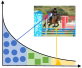
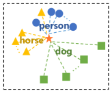
Long-tailed multi-label visual recognition (LTML)  [43, 11] is a common and practical task owing to the highly imbalanced data distribution  [50] and diverse objects of real-world images [41, 17]. Compared with long-tailed recognition and multi-label recognition task, LTML is more complex and challenging, because it requires capturing multiple categories and the label co-occurrence in individual images  [3, 17], which needs to compensate for the negative impacts caused by the long-tailed distribution (i.e., low performance on the tail classes).

Several approaches have been proposed to address the LTML problem from different perspectives, such as re-sampling  [1, 7, 11], re-weighting  [2, 43] and modeling more powerful structures  [3, 39, 41]. Despite their great contributions, these works neglect to take into account two crucial aspects. First of all, the importance of semantic feature interaction between classes to capture label co-occurrence. However, these methods are limited to balancing the distribution of categories from the perspective of samples, without considering the feature correlation between different classes. Second, synchronous improvements in head-to-tail category performance, while some of these works improve the performance of tail classes at the expense of the head classes.

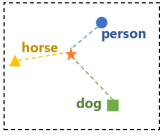
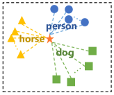
Recently, graphic models have been introduced to model the semantic label correlation in a few works [3, 39], whereas these works are complex and modeling label dependencies mainly based on the image modality without additional semantic information from other modal data. Vision-Language (VL) models  [27, 16, 37, 15] demonstrate the huge potential of text modality on semantic context feature for downstream visual tasks, especially for the prompt tuning methods [31, 33, 45], which provide an efficient way to transfer pre-trained VL models to downstream tasks by learning the task-specific prompts rather than finetuning the entire model. Nonetheless, the existing prompt tuning methods [53, 52, 35] for visual recognition simply minimize prediction errors using the classification loss (e.g., cross-entropy loss) with respect to the learnable prompts, which may lead to learning general embeddings or inaccurate class-related embeddings. For instance, as shown in Fig. 1, when presented with an image that contains both a head class $\left[\mathrm{person}\right]$ and a tail class $\left[\mathrm{horse}\right]$, the zero-shot method (Fig. 1) relies solely on the rich knowledge of the pre-trained VL model to assess the similarity between the image and the word embeddings of the class names, while the existing prompt tuning method (Fig. 1) further learns more generalized prompt tokens to improve model performance. However, these methods do not consider the inter-class relationships, particularly between head and tail classes, which is a critical factor for LTML. This underscores the need for approaches that incorporate such relationships to improve performance in such scenarios.

Therefore, to address these issues, we present the class-specific embedding loss for prompt tuning on long-tailed multi-label visual recognition, called LMPT. The abundance of image-caption data facilitates prompt learning that encompasses more nuanced and specific textual descriptions, as well as the semantic inter-dependencies between categories (Fig. 1) that share information, such as similar features or common descriptions. This attribute is particularly critical in the identification of both head and tail classes. More specifically, we propose the class-specific embedding loss to enhance the inclusivity of class-related embeddings within prompts. By gradually approaching the embeddings of the corresponding caption, our proposed approach enables prompt tokens to effectively judge the association between different classes with the aid of textual modality. Aiming for class imbalance and the consistency improvements between head classes and tail classes, we integrate class-aware soft margin and re-weighting into the class-specific embedding loss, which serves to assign larger margins and more weights to tail classes. Notably, for images containing both head and tail classes, our approach outperforms visual models and current prompt tuning methods. Moreover, we adopt the distribution-balanced loss [43] as the classification loss. To verify the effectiveness of our method, we conduct extensive experiments on the two benchmarks, including VOC-LT and COCO-LT [43, 21, 10]. Experimental results show that our method surpasses zero-shot CLIP [27] and previous SOTA [11] on the above benchmarks.

To sum up, the main contributions of this work include:

• We propose a novel LMPT framework to adapt pre-trained VL models (e.g., CLIP) to tackle long-tailed multi-label visual recognition, where text descriptions (captions) are easily accessible from public image-caption datasets or generated by powerful image-caption models [40].

• We present the class-specific embedding loss with class-aware soft margin and re-weighting to learn more fine-grained and class-related embeddings that build semantic relationships across head and tail classes with shared semantic information. Such design can benefit performance in tail classes and hard-to-recognize classes with the help of text modality.

• We verify the effectiveness of the proposed method on VOC-LT, and COCO-LT by achieving new state-of-the-art results on two data sets, which outperform previous SOTA [11] by 9 / 6 % and zero-shot CLIP by 6 / 2 % on VOC-LT / COCO-LT.

Figure 2: Overview of the architecture of our proposed method.

2 Related Work

2.1 Long-Tailed Visual Recognition

Real-world training data usually exhibits long-tailed distribution [50], which presents a challenge for traditional methods due to the imbalanced class distribution. To address this problem, several approaches [5, 25, 26, 30] have been proposed from different aspects. One common method is to directly re-sample the training data to balance the class distribution [9, 1, 7], by adjusting the sampling rate of head classes and tail classes, yet it might lead to the overfitting of tail classes. A better solution is to design re-weighted loss functions [19, 14, 2] that assign more weight to tail classes or ignore negative gradients [36] for tail classes. In addition, researchers also propose to use techniques such as transfer learning [23, 54] and self-supervised learning [18, 49] to alleviate the class imbalance problem. Recently, some studies [24, 37] also explore the possibility of text modality by refining visual-language representations on the long-tailed recognition tasks.

2.2 Multi-Label Visual Recognition

For multi-label visual recognition, some early methods include treating it as multiple binary image classifications [38, 48] or finding k-nearest neighbors [47]. To locate regions of interest, some researchers [39, 41] proposed to introduce recurrent neural networks (e.g., RNN, LSTM) to learn a joint image-label embedding. In addition, Chen et al. [3] proposed to model the label correlations by constructing a graph based on the label co-occurrence and Ye et al. [46] updated static graph to dynamic graph convolutional network (GCN) for robust representation. Wu et al. [43] proposed a distribution-balanced loss and Guo et al. [11] adopted collaborative training on the uniform and re-balanced samplings to alleviate the class imbalanced problem. There is also a popular trend to align between visual and textual features [44, 22, 15, 29] for multi-label recognition.

2.3 Prompt Tuning for Vision-Language Models

Prompt tuning [31, 33, 45] is a parameter-efficient technique used to utilize the representation ability of pre-trained vision-language models to achieve better performance instead of fine-tuning the whole model on downstream tasks. Meanwhile, large-scale vision-language models (e.g., CLIP [27], ALIGN [16]) have demonstrated impressive power to learn visual and textual features. CoOp [53] learns soft prompts via minimizing the classification loss and CoCoOp [52] further formulates the prompts in an image-conditional way to improve its generalization to unseen classes. DualCoOp [35] firstly adapts CLIP to multi-label image recognition by learning pairs of positive and negative prompts for each class. Different from the above work, LMPT focuses on exploring the transfer ability to address long-tailed multi-label visual recognition.

3 Methodology

In this section, we present our proposed prompting tuning method, i.e., LMPT, for adapting pre-trained vision-language models for long-tailed multi-label visual recognition.

3.1 Preliminaries

Consider $\mathcal{D}$ as the dataset we use, ${N}$ as the number of the dataset, $C$ as the number of classes, and $L$ as the fixed length of contexts for optimization. Then $(x^{k},y^{k},t^{k})\in\mathcal{D}_{train}$, ${k}\in\left\{1,...,N\right\}$, where $x^{k}$ is an input single image, $y^{k}=\left[y_{1}^{k},...,y_{C}^{k}\right]\in{\left\{0,1\right\}}^{C}$ is the multi-label ground-truth and $t^{k}=\left[t_{1}^{k},...,t_{L}^{k}\right]$ is the corresponding text embedding of text description (caption). But during the test phase, only $(x^{k},y^{k})\in\mathcal{D}_{test}$. Let $n_{i}=\sum_{k=1}^{N}y_{i}^{k}$ denote the number of training examples that contain class $i$. Please note that labels for computing the class-specific embedding loss need to be processed into $\tilde{y}^{k}=\left[\tilde{y}_{1}^{k},...,\tilde{y}_{C}^{k}\right]=\left[2*y_{1}^{k}-1,...,2*y_{C}^{k}-1\right]\in{\left\{-1,1\right\}}^{C}$, where $\left\{-1,1\right\}$ indicates negative and positive pairs respectively.

3.2 Approach Overview

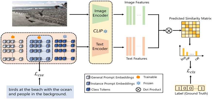
In order to make effective use of the linguistic modality in the long-tailed multi-label visual recognition task, we propose a novel framework (i.e., LMPT), as depicted in Fig. 2. Text encoder from the pre-trained CLIP is used to encode the prompts and text descriptions (captions) of images. Only the parameters in the prompts are optimized, while the text encoder and image encoder are both kept frozen. We introduce two sorts of trainable prompts to obtain class embedding, which are jointly optimized by the classification loss $\mathcal{L}_{cls}$ and class-specific embedding loss $\mathcal{L}_{cse}$. Details of the aforementioned loss functions will be introduced in the later sections.

3.3 Prompt Tuning

Formally, the vision-language model consists of an image encoder $\boldsymbol{f}(\cdot)$ and a text encoder $\boldsymbol{g}(\cdot)$. Following [52], a prompt is defined as:

$$o_{i}|_{1}^{M}=\left[\mathrm{V}\right]_{1}\left[\mathrm{V}\right]_{2}...\left[\mathrm{V}\right]_{m}...\left[\mathrm{V}\right]_{M}\left[\mathrm{CLASS}\right],$$ (1)

where $i\in\left\{1,...,C\right\}$, $m\in\left\{1,...,M\right\}$, the $\left[\mathrm{CLASS}\right]$ token is replaced by the specific class name (e.g., “cat,” “dog”, “car”), each $\left[\mathrm{V}\right]_{m}$ is a learnable word embedding with the same dimension as normal word embeddings in the vocabulary (i.e., 512 for CLIP), and $M$ is a hyper-parameter specifying the number of context tokens. The prediction probability (classification output) $z$ is then computed as:

$$p(y=i\mid x)=\frac{\exp\left(\cos\left(\boldsymbol{g}\left(o_{i}\right),\boldsymbol{f}\left(x\right)\right)/\tau\right)}{\sum_{j=1}^{C}\exp\left(\cos\left(\boldsymbol{g}\left(o_{j}\right),\boldsymbol{f}\left(x\right)\right)/\tau\right)},$$ (2)

where $\tau$ is a temperature parameter learned by CLIP and $cos(\cdot,\cdot)$ represents cosine similarity.

3.4 Class-Specific Embedding Loss

Inspired by hinge embedding loss [34] which is widely exploited for measuring whether two inputs are similar or not, we introduce the class-specific embedding (CSE) loss to optimize the trainable fine-grained instance prompts by learning from text embeddings of captions. It tries to minimize the cosine distance of matching patches and to increase the cosine distance of non-matching patches above the margin. Embedding loss is then computed as

$${\ell}_{ebd} =\begin{cases}\Delta_{i}^{k},&\text{if}\quad\tilde{y}_{i}^{k}=1,\\ \max\left(0,\mu-\Delta_{i}^{k}\right),&\text{if}\quad\tilde{y}_{i}^{k}=-1,\end{cases}$$ (3)

$$\Delta_{i}^{k}=1-\cos\left(t_{i}^{k},o_{i}|_{m}^{M}\right),$$

where $\mu$ is the margin factor. Intuitively the embedding loss penalizes positive (i.e., prompts of matching classes) pairs that have large distances and negative (i.e., prompts of non-matching classes) pairs that have small distance (less than $\mu$).

Figure 3: The class margins (dotted lines) are enforced for generated samples by updating the decision boundary with respect to class margins. Blue samples (head classes) are classified incorrectly and the model update gradient is shown with pointed arrows. Green samples (medium classes) are classified correctly outside of the margin and the gradient is shown. Therefore, the embedding loss does not give special consideration to the minority categories, but with the help of class-aware soft margin, the trade-off of $\mu_{1}$ can be optimized by shifting the decision boundary to encourage the tail classes to have larger margins. So yellow samples (tail classes) are classified correctly outside of the original margin but within the enlarged margin, and the embedding loss has no gradient for these samples.

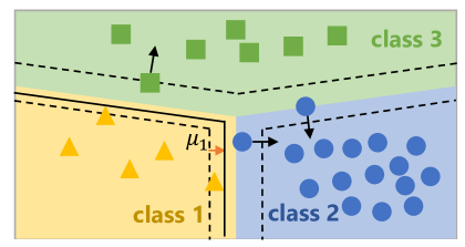
LDAM [2] has inspired the development of a decision boundary that is both robust and generalizable, capable of accurately classifying features that vary within a certain range. However, when applied to long-tailed datasets characterized by a significant class imbalance, models tend to exhibit greater sensitivity to more frequent classes. As a result, the performance of these models in less frequent classes is often poor. To address this issue, as illustrated in Fig. 3, CSE loss also incorporates the class-aware soft margin strategy to encourage the model to have the optimal trade-off between per-class margins by stimulating the minority classes to have larger margins, which can be viewed as regularization [42]. Following the trade-off between the class margins [2], we adopt a class-aware margin for multiple classes of the form

$$\widetilde{\mu_{i}}\propto n_{i}^{-1/4}=\frac{\eta}{n_{i}^{1/4}}.$$ (4)

Here $\eta$ is a hyper-parameter to be tuned. Therefore, when $y_{i}^{k}=-1$, the loss can be computed as $\max\left\{0,\widetilde{\mu_{i}}-\Delta_{i}^{k}\right\}$.

Meanwhile, our loss can be combined with a re-weighting strategy to be more efficient when it comes to long-tailed distribution data. We then define the reference weight based on the empirical class frequencies $\left\{n_{1},...,n_{C}\right\}$ on the training set:

$$w_{i}=\frac{\left(1/n_{i}\right)^{\gamma}}{\sum_{i=1}^{C}\left(1/n_{i}\right)^{\gamma}},$$ (5)

where $\gamma$ is a scale hyper-parameter to provide more flexibility. Hence, the re-weighted class-specific embedding loss is defined as:

$${\ell}_{cse} =\begin{cases}w_{i}\Delta_{i}^{k},&\text{if}\quad\tilde{y}_{i}^{k}=1,\\ \max\left\{0,w_{i}\left(\widetilde{\mu_{i}}-\Delta_{i}^{k}\right)\right\},&\text{if}\quad\tilde{y}_{i}^{k}=-1,\end{cases}$$ (6)

$$\mathcal{L}_{cse}=\frac{\sum_{k=1}^{N}{\ell}_{cse}}{N}.$$ (7)

3.5 Multi-Label Classification Loss

Our method can be easily combined with the existing multi-label classification loss functions [28, 20, 6, 43], regardless of whether they are designed for long-tailed distributions or not. By blending the classification loss functions with our proposed CSE loss, our method facilitates prompt learning of more refined class descriptions and semantic relationships between categories, particularly between head and tail classes.

In this study, we introduce the distribution-balanced loss [43] as the classification loss function, which can be formulated as:

$$r=\alpha+\sigma\left(\beta\times\left(\frac{\frac{1}{n_{i}}}{\sum_{i=1}^{C}\frac{1}{n_{i}}}-\theta\right)\right),$$ (8)

$$v_{i}=-\kappa\times-\log\left(\frac{1}{n_{i}/N}-1\right),$$ (9)

$${\ell}_{cls} =\begin{cases}-r\left(1-q_{i}^{k}\right)^{\gamma}\log\left(q_{i}^{k}\right),&\text{if}\quad y_{i}^{k}=1,\\ -\frac{r}{\zeta}\left(q_{i}^{k}\right)^{\gamma}\log\left(1-q_{i}^{k}\right),&\text{if}\quad y_{i}^{k}=-1,\end{cases}$$ (10)

where $q_{i}^{k}=\sigma\left(z_{i}^{k}-v_{i}\right)$ is for positive instances, $q_{i}^{k}=\sigma\left(\zeta\left(z_{i}^{k}-v_{i}\right)\right)$ is for negative ones and $\alpha,\beta,\theta,\kappa,\zeta$ are hyperparameters. Then $\mathcal{L}_{cls}=\sum_{k=1}^{N}{\ell}_{cls}/N$.

Hence, the overall training loss can be written as:

$$\mathcal{L}=\lambda\mathcal{L}_{cls}+\left(1-\lambda\mathcal{L}_{cse}\right),$$ (11)

where $\lambda\in[0,1]$ is a hyperparameter to balance $\mathcal{L}_{cls}$ and $\mathcal{L}_{cse}$.

Datasets	VOC-LT				COCO-LT
Methods	total	head	medium	tail	total	head	medium	tail
Backbone: RN-50
ERM	70.86	68.91	80.20	65.31	41.27	48.48	49.06	24.25
RW	74.70	67.58	82.81	73.96	42.27	48.62	45.80	32.02
Focal Loss [20]	73.88	69.41	81.43	71.56	49.46	49.80	54.77	42.14
RS [32]	75.38	70.95	82.94	73.05	46.97	47.58	50.55	41.70
ML-GCN [4]	68.92	70.14	76.41	62.39	44.24	44.04	48.36	38.96
OLTR [23]	71.02	70.31	79.80	64.95	45.83	47.45	50.63	38.05
LDAM [2]	70.73	68.73	80.38	69.09	40.53	48.77	48.38	22.92
CB Focal [6]	75.24	70.30	83.53	72.74	49.06	47.91	53.01	44.85
BBN [51]	73.37	71.31	81.76	68.62	50.00	49.79	53.99	44.91
DB Focal [43]	78.94	73.22	84.18	79.30	53.55	51.13	57.05	51.06
LTML [11]	81.44	75.68	85.53	82.69	56.90	54.13	60.59	54.47
[1pt/1pt] Zero-Shot CLIP	84.30	63.60	88.03	97.03	56.19	35.73	60.52	68.45
CoOp [53]	81.34	65.10	81.54	93.37	54.94	38.06	56.67	67.51
CoCoOp [52]	78.63	64.33	80.51	87.94	46.02	36.02	50.57	48.82
DualCoOp [35]	81.03	66.45	80.53	92.33	53.11	40.48	55.20	62.11
LMPT (ours)	85.44	66.62	88.11	97.86	58.97	41.87	61.60	69.60
Backbone: ViT-B/16
Zero-Shot CLIP	85.77	66.52	88.93	97.83	60.17	38.52	65.06	72.28
CoOp [53]	86.02	67.71	88.79	97.67	60.68	41.97	63.18	73.85
CoCoOp [52]	84.47	64.58	87.82	96.88	61.49	39.81	64.63	76.42
LMPT (ours)	87.88	72.10	89.26	98.49	66.19	44.89	69.80	79.08

Table 1: mAP performance of the proposed method and comparison methods. Above the dotted line is the performance of visual models and below is that of vision-language models.

4 Experiments

4.1 Datasets

Following [43], we conduct experiments on two datasets for long-tailed multi-label visual recognition: VOC-LT and COCO-LT [43]. They are artificially sampled from two multi-label recognition benchmarks, PascalVOC [10] and MS-COCO [21], respectively.

VOC-LT is created from the 2012 train-val set of PascalVOC based on the settings in [43]. The training set contains 1,142 images and 20 class labels, and the number of images per class ranges from 4 to 775. All the classes are split into three groups according to the number of training samples per class: a head class has more than 100 samples, a medium class has 20 to 100 samples, and a tail class has less than 20 samples. The ratio of head, medium, and tail classes after splitting is 6:6:8. The text description of each image in the training set is generated by OFA [40]. VOC2007 test set with 4,952 images is used to evaluate the performance as the test set.

COCO-LT is constructed from MS-COCO 2017 in a similar way. The training set of this dataset contains 1,909 images and 80 class labels, and the number of images per class ranges from 6 to 1,128. The ratio of head, medium, and tail classes is 22:33:25 in COCO-LT. We use captions as text descriptions of each image in the training set from MS-COCO which is a public image caption dataset as well. The test set is MS-COCO 2017 test set with 5,000 images.

4.2 Experimental Settings

Evaluation Metrics. As in [23], the classes are split into three groups by the number of their training examples: head classes each contain over 100 samples, medium classes each has between 20 and 100 samples, and tail classes with under 20 samples each. We use mean average precision (mAP) to evaluate the performance of long-tailed multi-label visual recognition for all the classes.

Implementation Details. We adopt CLIP ResNet-50 [13] or ViT-Base/16 [8] as the visual encoder and use the corresponding CLIP Transformer as the text encoder. During training, the parameters of both the two encoders are kept frozen, and only learnable prompts are optimized. SGD optimizer is adopted to learn prompt tokens, and the training epochs are set to 30. The learning rates for COCO-LT, and VOC-LT are empirically initialized with 1e-4, 5e-4, and decay by the cosine annealing rule during training. For loss functions, $\eta$ in Eq. 4, $\gamma$ in Eq. 5 and $\lambda$ in Eq. 11 are set as 1.0, 1.0 and 0.5, respectively. Other hyperparameters in DB loss are set as the same as [43]. All the experiments are implemented on PyTorch 1.13.0 using an NVIDIA GeForce RTX 3090 GPU.

4.3 Comparison with Prior SOTA Works

To evaluate the effectiveness of the proposed method, firstly we compare it with previous methods of visual models on the two long-tailed multi-label datasets. The compared methods include Empirical Risk Minimization (ERM), a smooth version of Re-Weighting (RW) using the inverse proportion to the square root of class frequency, Re-Sampling (RS) [32], Focal Loss [20], ML-GCN [4], OLTR [23], LDAM [2], Class-Balanced (CB) Focal [6], BBN [51], Distribution-Balanced (DB) Focal [43] and LTML [11]. The mAP performance of different methods is shown in Table 1. The prior best performance is achieved by LTML – mAP of 81.44% over all classes on VOC-LT and 56.90% over all classes on COCO-LT.

Furthermore, we compare zero-shot and few-shot methods based on CLIP on the two benchmarks. The mAP performance of these methods is shown in Table 1 as well. For a fair comparison, we initialize the prompt as the default hand-crafted one “a photo of a” for all the methods. The results show that when using ViT-Base/16 as the backbone, even the overall mAP performance of zero-shot CLIP reaches 85.77% and 60.17%, which outperforms previous SOTA LTML by 4.33 points (85.77% vs.81.44%) and 3.27 points (60.17% vs.56.90%) on the two datasets, respectively. Therefore, it is meaningful to explore how to use prompt tuning based on CLIP effectively for better performance. From the perspective of prompt tuning methods, when using ResNet-50 as the backbone, the performance of our method on VOC-LT is more promising, which is 4.1 points, 6.81 points and 4.41 points better than CoOp [53], CoCoOp [52] and DualCoOp [35], which are popular prompt learning methods for single-label and multi-label recognition. And the performance on COCO-LT is similar to that on VOC-LT, which is 4.03 points, 12.95 points, and 5.86 points better than CoOp, CoCoOp and DualCoOp. When replacing the backbone with ViT-Base/16, the overall mAP performance of our method can further boost up to 87.88% and 66.19% on VOC-LT and COCO-LT, which is the current new state-of-the-art of the two datasets.

Datasets	VOC-LT
Methods	total	head	medium	tail
BCE	82.18	64.90	83.17	94.30
MLS	84.30	64.31	84.82	97.47
Focal Loss [20]	85.37	66.17	87.70	97.52
CB Loss [6]	85.25	65.37	87.71	97.20
R-BCE-Focal [43]	84.56	66.01	86.61	97.67
ASL [28]	86.40	69.12	88.79	98.07
DB Focal [43]	87.88	72.10	89.26	98.49

Datasets	COCO-LT
Methods	total	head	medium	tail
BCE	58.04	41.79	58.86	73.90
MLS	61.26	41.71	64.11	74.58
Focal Loss [20]	54.40	37.60	59.36	62.33
CB Loss [6]	56.45	34.61	58.77	74.52
R-BCE-Focal [43]	60.13	38.11	64.87	72.79
ASL [28]	64.89	43.18	68.22	78.43
DB Focal [43]	66.19	44.89	69.80	79.08

Table 2: mAP performance of the proposed method with different multi-label loss functions.

4.4 Ablation Analysis

Components Analysis. To further analyze which component makes our methods performant for long-tailed multi-label recognition, we conduct a set of ablation studies and report the results in Table 3. We first conduct experiment with zero-shot CLIP and the achieved mAP performances are 85.77% on VOC-LT, 60.17% on COCO-LT, which surprisingly outperforms the prior SOTA LTML. It indicates that pre-trained VL models demonstrate a robust capability for visual recognition, providing a solid foundation for our approach. However, the mAP performance of the tail classes outperforms head classes by nearly 30 points on both VOC-LT and COCO-LT. Then CoOp benefited from soft prompts (learnable prompts) and the mAP performance is improved to 86.02% on VOC-LT and 60.68% on COCO-LT, with 0.25% and 0.51% increments. Besides, we design the class-specific embedding (CSE) loss with class-aware soft margin (CASM) and re-weighting (RW) to learn more fine-grained and class-related prompts that build semantic relationships across different classes, especially for the tail classes by encouraging those classes to have larger margins and weights. The mAP performances of head, medium, and tail classes after adding the embedding loss are all significantly improved and the overall mAP surpasses CoOp by 1.26% and 4.66% on VOC-LT and COCO-LT, which demonstrates our embedding loss can help prompts learn fine-grained classes descriptions and semantic relationships across the classes. Finally, the integration of CASM and RW strategy further improves the mAP performance slightly, mainly for the tail performance by 0.65% and 1.12% on VOC-LT and COCO-LT.

SP	EBD	CASM	RW	VOC-LT				avg.$\Delta$	COCO-LT				avg.$\Delta$
				total	head	medium	tail		total	head	medium	tail
				85.77	66.52	88.93	97.83		60.17	38.52	65.06	72.28
✓				86.02	67.71	88.79	97.67	+0.29	60.68	41.97	63.18	73.85	+0.91
✓	✓			87.28	71.07	89.01	97.84	+0.51	65.34	44.27	69.39	77.96	+5.23
✓	✓	✓		87.62	72.01	89.26	98.13	+1.99	65.81	44.90	69.71	78.76	+5.79
✓	✓	✓	✓	87.88	72.10	89.26	98.49	+2.17	66.19	44.89	69.80	79.08	+5.98

Table 3: Ablation analysis on different components of the proposed method. Here “SP” denotes Soft Prompt, “EBD” Embedding Loss, “CASM” Class-Aware Soft Margin, “RW” Re-weighting, “avg.$\Delta$” average performance improvement.

Multi-Label Classification Loss Functions. Here, we compare a number of multi-label classification loss functions, including Binary Cross-Entropy Loss (BCE), Multi-Label Soft Margin Loss (MSL), Focal Loss [20], CB Loss [6], R-BCE-Focal [43], Asymmetric Loss (ASL) [28] and DB Focal [43]. As illustrated in Table 2, DB Focal loss that takes the co-occurrence of labels and the dominance of negative labels into account works significantly better than other multi-label classification loss for the long-tailed multi-label visual recognition task.

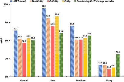
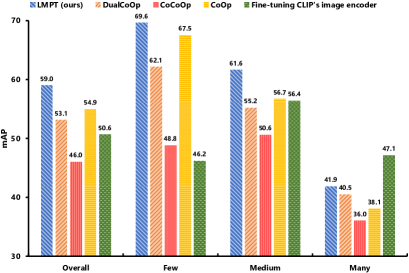
Effectiveness of Text Supervision. We further compare our method with fine-tuning CLIP’s image encoder when using ResNet-50 as the backbone to explore whether the significant effect of our approach is due to text supervision or simply because the CLIP’s image encoder is so powerful. In order to prevent interference with the trained CLIP’s image encoder during the fine-tuning phase, we only fine-tune a fully connected layer added at the end of the image encoder. The results are shown in Fig. 4. Obviously, fine-tuning the image encoder shows promising results, but still largely underperforms LMPT, which suggests that the gradients that went through the text encoder provide more useful information.

Figure 4: mAP performance of different methods w/o text supervision on two datasets.  (a) VOC-LT. (b) COCO-LT.

Figure 5: Example decisions from our model, CLIP and ResNet.

4.5 Qualitative Analysis

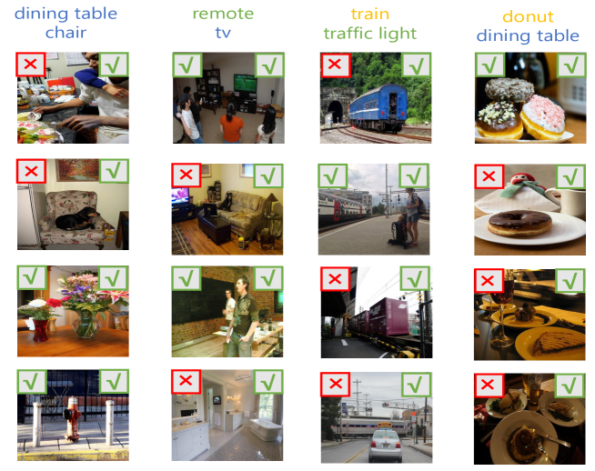
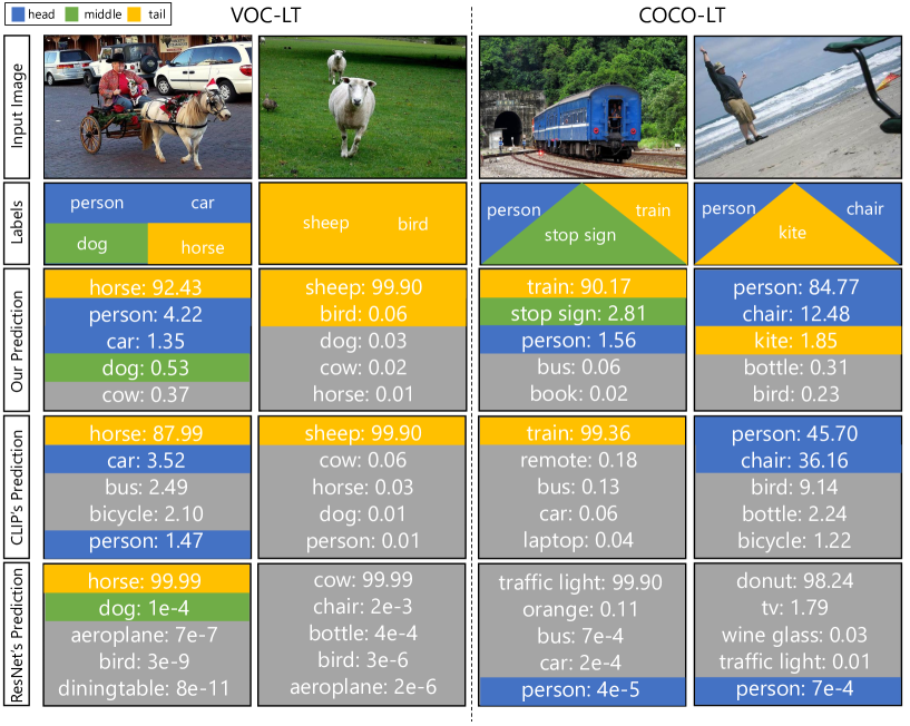
To better understand how our method deals with long-tailed multi-label data, we performed qualitative experiments with ResNet, CLIP, and ours on COCO-LT and VOC-LT. Fig. 5 shows several cases where the model justifies its abilities for the prediction. For example, in the third column, ResNet only recognizes $\left[\mathrm{person}\right]$ (belongs to head classes) and fails to classify the image to $\left[\mathrm{train}\right]$ (belongs to tail classes), which is a pervasive challenge encountered by visual models. The emergence of CLIP is a great remedy for this issue, owing to its huge training data and effective text supervision. Nevertheless, simple hand-crafted templates as prompts still cannot accurately identify categories as they cannot describe the characteristics of each category. Understanding the inter-class relationships, particularly among head and tail categories, presents a formidable challenge in multi-label visual recognition, which is essential for achieving optimal performance in this domain. With the aid of our approach, utilizing prompts that learn from a large corpus of image-caption data, it has become feasible to discern the semantic relationships between categories and accurately predict the relevant categories of simple objects, even in challenging scenarios such as identifying $[\mathrm{stop}$ $\mathrm{sign}]$ from images. Therefore, our proposed method demonstrates significant advantages in effectively addressing the intricate relationship among multiple labels and the long-tailed problem with the aid of text supervision.

4.6 Limitations

Although the proposed method LMPT achieves good performance on two long-tailed multi-label recognition benchmarks, it still has some imperfections. Firstly, text descriptions in VOC-LT are generated by the open-source image-caption model, which inevitably leads to some inaccurate texts. Secondly, although captions and labels in COCO-LT are manually annotated, there are still many errors (e.g., missing label words in the text, inconsistent labels), which greatly affects the performance of the model. Moreover, VL models underperform prior visual models overhead classes significantly, which demonstrates that there is much room for improvement in the current VL models. However, we believe that advancements in VL models and text data will lead to solutions for these challenges in the future.

5 Conclusion

In this work, we propose a new view of prompt tuning for long-tailed multi-label visual recognition by learning class-specific contexts from the alignment of prompts and textual description (caption), which complements more fine-grained features and builds semantic relationships across head and tail classes. Considering the class imbalance, the class-specific embedding loss is added with the class-aware soft margin and re-weighting strategy to encourage the tail classes to be more generalized. Furthermore, we adopt distribution-balanced loss as the classification loss function, which is more suitable for our task compared with other loss functions. Our method demonstrates substantial improvement over the previous SOTA and zero-shot CLIP on VOC-LT and COCO-LT. We hope our approach will inspire future work in this field.

Supplementary Document

6 Prompt Initialization

We compare random initialization with manual initialization. The latter uses the embeddings of “a photo of a” to initialize the context vectors for the two datasets. For a fair comparison, we also set the context length to 4 when using random initialization. Table 4 suggests that in the case of a small-scale training set (e.g., VOC-LT: 1.9k+ images) a good initialization has a big impact. The model performance may be better if we use the initialization words for a specific dataset for further optimization.

	Total	Head	Medium	Tail
$\left[\mathrm{V}\right]_{1}\left[\mathrm{V}\right]_{2}\left[\mathrm{V}\right]_{3}\left[\mathrm{V}\right]_{4}$	84.74	65.73	87.23	97.13
“a photo of a”	87.88	72.10	89.26	98.49

Table 4: Random v.s. manual initialization.

7 Comparison with Prompt Ensembling

Radford et al. [27] proposed that ensembling over multiple zero-shot classifiers generated using different hand-crafted prompts can improve performance, such as “a photo of the large [CLASS].”, “a bad photo of the [CLASS].”, which represent different scales and views for images. The 80 context prompts are selected for experiments, which have been demonstrated their usefulness on ImageNet. The used templates are listed in “prompt_template.py”. As shown in Table 5, there is a slight increase in model performance over the single-template prompt method on certain datasets, but justifies the superiority of LMPT.

Dataset	Method	mAP (%)
		Total	Head	Medium	Tail
VOC-LT	Zero-Shot	85.77	66.52	88.93	97.83
	Ensembling	85.17	65.57	88.36	97.45
	LMPT	87.88	72.10	89.26	98.49
COCO-LT	Zero-Shot	60.17	38.52	65.06	72.28
	Ensembling	60.86	41.14	65.21	72.47
	LMPT	66.19	44.89	69.80	79.08

Table 5: Comparison with prompt engineering and prompt ensembling. The best and second-best performance are indicated by bold and underline, respectively.

8 Prompt Length

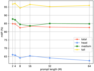
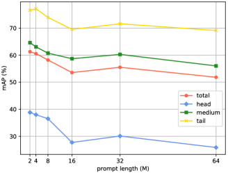
Overall Prompt Length $M$. As shown in Fig. 6, we have provided the comparison of the performance of LMPT with different prompt context lengths (i.e., $M=2,4,8,16,32,64$) in the two datasets. For long-tailed multi-label visual recognition, we learn class-specific prompts and thus LMPT performs well when $M$ is small, such as $2,4$.

Figure 6: Results (mAP %) with different prompt length $M$ for computing classification loss.  (a) VOC-LT. (b) COCO-LT.

Prompt Length $m$ for Computing CSE Loss. Moreover, we also compare with different lengths $m$ of prompt context to compute the class-specific embedding loss $\left(m\leq M\right)$. Table 6 shows that LMPT performs the best when $m/M=25\%$ on the two datasets, which is quite reasonable. Only a small fraction of tokens is required to learn the general prompts (e.g., “a photo of a”), as they are not very complex and do not require many tokens to represent. However, more tokens are needed to learn the class-specific prompts, because more tokens are needed to describe the categories and the semantic relationships between them. The prompts cannot fully capture the class descriptions and semantic relationships if the number of tokens is relatively small.

Dataset	$m/M$	mAP (%)
		Total	Head	Medium	Tail
VOC-LT	12.5%	82.35	63.08	82.83	96.43
	25%	83.56	64.06	84.22	97.59
	50%	82.43	62.52	83.86	96.30
	75%	82.01	61.46	83.85	96.06
	100%	83.32	65.34	83.60	96.59
COCO-LT	12.5%	51.89	26.61	56.01	68.71
	25%	56.16	31.29	60.46	72.38
	50%	52.15	26.56	56.09	69.47
	75%	54.14	29.34	57.28	71.81
	100%	53.55	27.71	58.67	69.53

Table 6: Performance with different settings of prompt length $m$. The performance reported here is the average performance when $M=16$.

9 Algorithm of Class-Specific Embedding Loss

The overall process of class-specific embedding loss is outlined in Algorithm 1.

Input: Text embeddings of textual descriptions (captions) $t$, labels $\widetilde{y}$, prompt $o$

Output: Class-Specific Embedding Loss $\mathcal{L}_{cse}$

1 for $k=1,2,...,N$ do

2       $\ell_{cse}=0$;

3       for $i=1,2,...,C$ do

4             Compute class-aware soft margin $\widetilde{\mu}_{i}$ using Eq. (4);

5             Compute weight $w_{i}$ using Eq. (5);

6             Compute $\Delta_{i}^{k}=1-\cos\left(t_{i}^{k},o_{i}|_{m}^{M}\right)$;

7             if $\widetilde{y}_{i}^{k}=1$ then

8                   $\ell_{cse}=w_{i}\Delta_{i}^{k}$;

9                  

10            else

11                   $\ell_{cse}=\text{ReLU}\left(w_{i}\left(\widetilde{\mu}_{i}-\Delta_{i}^{k}\right)\right)$;

12                  

13             end if

14            

15       end for

16      

17 end for

Compute $\mathcal{L}_{cse}$ using Eq. (7).

Algorithm 1 Class-Specific Embedding Loss

10 Comparison with Fine-tuning CLIP

We try to fine-tune the entire CLIP model and find that in the first epoch of fine-tuning, there is a slight improvement in model performance, with an increase in the head classes but a decrease in the tail classes. However, as shown in Table 7, in the following epochs, the performance gradually deteriorates in the following epochs. Therefore, fine-tuning CLIP is far inferior to LMPT, which can simultaneously improve the performance of both head and tail classes.

Dataset	Method	mAP (%)
		Total	Head	Medium	Tail
VOC-LT	Zero-Shot	85.77	66.52	88.93	97.83
	FT (Epoch 1)	86.77	70.05	90.32	96.63
	FT (Epoch 2)	85.26	66.55	89.42	96.17
	FT (Epoch 3)	85.67	67.32	89.78	96.34
	FT (Epoch 4)	84.80	65.83	88.52	96.23
	FT (Epoch 5)	85.35	67.00	89.35	96.12
	LMPT	87.88	72.10	89.26	98.49
COCO-LT	Zero-Shot	60.17	38.52	65.06	72.28
	FT (Epoch 1)	58.72	40.55	62.67	69.50
	FT (Epoch 2)	58.44	40.33	62.63	68.86
	FT (Epoch 3)	57.83	39.76	61.74	68.75
	FT (Epoch 4)	55.67	36.89	59.30	67.41
	FT (Epoch 5)	52.12	33.09	56.62	62.93
	LMPT	66.19	44.89	69.80	79.08

Table 7: Comparison with fine-tuning CLIP. “FT” denotes fine-tuning.

11 Analysis of Multi-Label Classification Loss Functions

Below we discuss the connections between some common multi-label classification loss functions. The standard formula for the multi-label classification loss function is as follows:

$${\ell}_{cls} =\begin{cases}{\ell}_{cls+}=-w\left(1-p_{+}\right)^{\gamma}\log\left(p_{+}\right),\\ {\ell}_{cls-}=-w\left(p_{-}\right)^{\gamma}\log\left(1-p_{-}\right),\end{cases}$$ (12)

where $w$ denotes weight, $\gamma$: scale hyper-parameter, $p_{+},p_{-}$: prediction probability for positive and negative instances. Detailed comparison is reported in Table 8. Hence, we apply the distribution-balanced loss [43] as the classification loss function, which integrates rebalanced weighting and negative-tolerant regularization for long-tailed multi-label recognition.

Methods	$\gamma$	$w$	$p_{+}$	$p_{-}$
BCE	-	-	$\sigma\left(z\right)$	$\sigma\left(z\right)$
FL [20]	$\gamma$	-	$\sigma\left(z\right)$	$\sigma\left(z\right)$
CB [6]	$\gamma$	$\frac{1-\beta}{1-\beta^{n}}$	$\sigma\left(z\right)$	$\sigma\left(z\right)$
ASL [28]	$\gamma_{+},\gamma_{-}$	-	$\sigma\left(z\right)$	$\max\left(\sigma\left(z\right)-m,0\right)$
DB [43]	$\gamma$	$\alpha+\sigma\left(\beta\frac{\frac{1}{n}}{\sum\frac{1}{n}}-\theta\right)$	$\sigma\left(z-v\right)$	$\sigma\left(\zeta\left(z-v\right)\right)$

Table 8: Comparison with the exsiting multi-label classification loss functions. $\alpha,\beta,m,\zeta,\kappa$: hypper-parameter, $v$: class-specific bias calculated by $\sigma\left(z\right)$ and $\kappa$, $\sigma$: sigmoid function.

Dataset	Method	#P	mAP (%)
			Total	Head	Medium	Tail
VOC-LT	Zero-Shot	-	84.30	63.60	88.03	97.03
	CoOp [52]	$P$	81.34	65.10	81.54	93.37
	TaI-DPT [12]	$2P$	83.75	66.27	85.17	94.57
	DualCoOp [35]	$2P$	81.03	66.45	80.53	92.33
	LMPT	$P$	85.44	66.62	88.11	97.86
COCO-LT	Zero-Shot	-	56.19	35.73	60.52	68.45
	CoOp [52]	$P$	54.94	38.06	56.67	67.51
	TaI-DPT [12]	$2P$	56.23	40.52	58.40	66.09
	DualCoOp [35]	$2P$	53.11	40.48	55.20	62.11
	LMPT	$P$	58.97	41.87	61.60	69.60

Table 9: Comparison with TaI-DPT and DualCoOp. “#P” denotes the number of parameters that the model needs to update. The reported performances here all use ResNet-50 as the backbone for a fair comparison.

12 Loss Weight $\lambda$

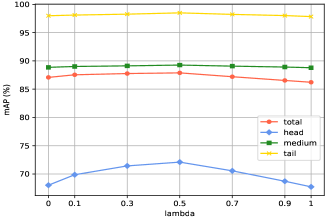
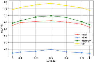
As shown in Fig. 7, we compare the model performance under different settings of loss weight $\lambda$ in the two loss functions, and the results show that when lambda is set to 0.5, the two loss functions can be better balanced, resulting in the best model performance.

Figure 7: Results (mAP %) with different weight $\lambda$.  (a) VOC-LT. (b) COCO-LT.

13 Comparison with DualCoOp and TaI-DPT

In this section, we aim to analyze and compare two methods that adapt pre-trained CLIP for multi-label recognition tasks. DualCoOp [35] proposes to use a pair of positive and negative prompts to generate binary classification probability for each class through contrastive learning. Table 9 suggests that the negative prompt is not able to handle long-tailed multi-label visual recognition effectively. While it can significantly improve the performance of the head classes, it can cause a substantial drop in the performance of the tail classes. In addition, TaI-DPT [12] suggests using double-grained prompts to focus on global and local features separately, which has a certain effect on multi-label visual recognition, but it cannot alleviate the long-tailed problem, and the performance on the tail classes still decreases.

However, for our proposed prompt tuning with class-specific embedding (CSE) loss, a single prompt is used to learn both class-related descriptions and semantic relationships between categories, instead of using two prompts as used in DualCoOp and TaI-DPT, which reduces the number of parameters the model needs to train. The class-specific contexts with the benefit of textual descriptions (captions) can help establish semantic relationships between classes, especially between the head and tail classes. Furthermore, the CSE loss, which incorporates class-aware soft margin and re-weighting, allows the model to pay more attention to the tail classes without sacrificing the performance on the head classes. As a result, we achieve state-of-the-art performance on this task.

14 More Examples

In this section, we provide four sets of images containing two labels with semantic relationships to further compare the performance of CLIP and LMPT (ours). And the selected labels include not only the head classes but also the tail classes, which comprehensively demonstrates the superiority of LMPT. As shown in Fig. 8, whether it is two head classes with semantic relationship, or one head class and one tail class, or one medium class and one tail class, LMPT can cover more visual attributes than CLIP due to the advantages of CSE loss.

Figure 8: More examples of our model and CLIP. The correctness of the judgement of each image depends on whether the two labels with semantic relationships are within the top 10 predicted labels of the model. The top left is CLIP’s judgment, and the top right is ours. The color of the labels corresponds to whether they belong to the head, medium, and tail classes.

References

- [1] Mateusz Buda, Atsuto Maki, and Maciej A Mazurowski. A systematic study of the class imbalance problem in convolutional neural networks. Neural networks, 106:249–259, 2018.
- [2] Kaidi Cao, Colin Wei, Adrien Gaidon, Nikos Arechiga, and Tengyu Ma. Learning imbalanced datasets with label-distribution-aware margin loss. Advances in neural information processing systems, 32, 2019.
- [3] Tianshui Chen, Muxin Xu, Xiaolu Hui, Hefeng Wu, and Liang Lin. Learning semantic-specific graph representation for multi-label image recognition. In Proceedings of the IEEE/CVF international conference on computer vision, pages 522–531, 2019.
- [4] Zhao-Min Chen, Xiu-Shen Wei, Peng Wang, and Yanwen Guo. Multi-label image recognition with graph convolutional networks. In Proceedings of the IEEE/CVF conference on computer vision and pattern recognition, pages 5177–5186, 2019.
- [5] Jiequan Cui, Shu Liu, Zhuotao Tian, Zhisheng Zhong, and Jiaya Jia. Reslt: Residual learning for long-tailed recognition. IEEE Transactions on Pattern Analysis and Machine Intelligence, 2022.
- [6] Yin Cui, Menglin Jia, Tsung-Yi Lin, Yang Song, and Serge Belongie. Class-balanced loss based on effective number of samples. In Proceedings of the IEEE/CVF conference on computer vision and pattern recognition, pages 9268–9277, 2019.
- [7] Qi Dong, Shaogang Gong, and Xiatian Zhu. Class rectification hard mining for imbalanced deep learning. In Proceedings of the IEEE International Conference on Computer Vision, pages 1851–1860, 2017.
- [8] Alexey Dosovitskiy, Lucas Beyer, Alexander Kolesnikov, Dirk Weissenborn, Xiaohua Zhai, Thomas Unterthiner, Mostafa Dehghani, Matthias Minderer, Georg Heigold, Sylvain Gelly, et al. An image is worth 16x16 words: Transformers for image recognition at scale. arXiv preprint arXiv:2010.11929, 2020.
- [9] Chris Drummond, Robert C Holte, et al. Class imbalance, and cost sensitivity: why under-sampling beats over-sampling. In Workshop on learning from imbalanced datasets II, volume 11, pages 1–8, 2003.
- [10] Mark Everingham, SM Eslami, Luc Van Gool, Christopher KI Williams, John Winn, and Andrew Zisserman. The pascal visual object classes challenge: A retrospective. International journal of computer vision, 111(1):98–136, 2015.
- [11] Hao Guo and Song Wang. Long-tailed multi-label visual recognition by collaborative training on uniform and re-balanced samplings. In Proceedings of the IEEE/CVF Conference on Computer Vision and Pattern Recognition, pages 15089–15098, 2021.
- [12] Zixian Guo, Bowen Dong, Zhilong Ji, Jinfeng Bai, Yiwen Guo, and Wangmeng Zuo. Texts as images in prompt tuning for multi-label image recognition. arXiv preprint arXiv:2211.12739, 2022.
- [13] Kaiming He, Xiangyu Zhang, Shaoqing Ren, and Jian Sun. Deep residual learning for image recognition. In Proceedings of the IEEE conference on computer vision and pattern recognition, pages 770–778, 2016.
- [14] Chen Huang, Yining Li, Chen Change Loy, and Xiaoou Tang. Learning deep representation for imbalanced classification. In Proceedings of the IEEE conference on computer vision and pattern recognition, pages 5375–5384, 2016.
- [15] Xinyu Huang, Youcai Zhang, Ying Cheng, Weiwei Tian, Ruiwei Zhao, Rui Feng, Yuejie Zhang, Yaqian Li, Yandong Guo, and Xiaobo Zhang. Idea: Increasing text diversity via online multi-label recognition for vision-language pre-training. In Proceedings of the 30th ACM International Conference on Multimedia, pages 4573–4583, 2022.
- [16] Chao Jia, Yinfei Yang, Ye Xia, Yi-Ting Chen, Zarana Parekh, Hieu Pham, Quoc Le, Yun-Hsuan Sung, Zhen Li, and Tom Duerig. Scaling up visual and vision-language representation learning with noisy text supervision. In International Conference on Machine Learning, pages 4904–4916. PMLR, 2021.
- [17] Lie Ju, Xin Wang, Zhen Yu, Lin Wang, Xin Zhao, and Zongyuan Ge. Long-tailed multi-label retinal diseases recognition using hierarchical information and hybrid knowledge distillation. arXiv preprint arXiv:2111.08913, 2021.
- [18] Bingyi Kang, Yu Li, Sa Xie, Zehuan Yuan, and Jiashi Feng. Exploring balanced feature spaces for representation learning. In International Conference on Learning Representations, 2020.
- [19] Salman H Khan, Munawar Hayat, Mohammed Bennamoun, Ferdous A Sohel, and Roberto Togneri. Cost-sensitive learning of deep feature representations from imbalanced data. IEEE transactions on neural networks and learning systems, 29(8):3573–3587, 2017.
- [20] Tsung-Yi Lin, Priya Goyal, Ross Girshick, Kaiming He, and Piotr Dollár. Focal loss for dense object detection. In Proceedings of the IEEE international conference on computer vision, pages 2980–2988, 2017.
- [21] Tsung-Yi Lin, Michael Maire, Serge Belongie, James Hays, Pietro Perona, Deva Ramanan, Piotr Dollár, and C Lawrence Zitnick. Microsoft coco: Common objects in context. In European conference on computer vision, pages 740–755. Springer, 2014.
- [22] Shilong Liu, Lei Zhang, Xiao Yang, Hang Su, and Jun Zhu. Query2label: A simple transformer way to multi-label classification. arXiv preprint arXiv:2107.10834, 2021.
- [23] Ziwei Liu, Zhongqi Miao, Xiaohang Zhan, Jiayun Wang, Boqing Gong, and Stella X Yu. Large-scale long-tailed recognition in an open world. In Proceedings of the IEEE/CVF Conference on Computer Vision and Pattern Recognition, pages 2537–2546, 2019.
- [24] Teli Ma, Shijie Geng, Mengmeng Wang, Jing Shao, Jiasen Lu, Hongsheng Li, Peng Gao, and Yu Qiao. A simple long-tailed recognition baseline via vision-language model. arXiv preprint arXiv:2111.14745, 2021.
- [25] Aditya Krishna Menon, Sadeep Jayasumana, Ankit Singh Rawat, Himanshu Jain, Andreas Veit, and Sanjiv Kumar. Long-tail learning via logit adjustment. arXiv preprint arXiv:2007.07314, 2020.
- [26] Wanli Ouyang, Xiaogang Wang, Cong Zhang, and Xiaokang Yang. Factors in finetuning deep model for object detection with long-tail distribution. In Proceedings of the IEEE conference on computer vision and pattern recognition, pages 864–873, 2016.
- [27] Alec Radford, Jong Wook Kim, Chris Hallacy, Aditya Ramesh, Gabriel Goh, Sandhini Agarwal, Girish Sastry, Amanda Askell, Pamela Mishkin, Jack Clark, et al. Learning transferable visual models from natural language supervision. In International Conference on Machine Learning, pages 8748–8763. PMLR, 2021.
- [28] Tal Ridnik, Emanuel Ben-Baruch, Nadav Zamir, Asaf Noy, Itamar Friedman, Matan Protter, and Lihi Zelnik-Manor. Asymmetric loss for multi-label classification. In Proceedings of the IEEE/CVF International Conference on Computer Vision, pages 82–91, 2021.
- [29] Tal Ridnik, Gilad Sharir, Avi Ben-Cohen, Emanuel Ben-Baruch, and Asaf Noy. Ml-decoder: Scalable and versatile classification head. In Proceedings of the IEEE/CVF Winter Conference on Applications of Computer Vision, pages 32–41, 2023.
- [30] Dvir Samuel and Gal Chechik. Distributional robustness loss for long-tail learning. In Proceedings of the IEEE/CVF International Conference on Computer Vision, pages 9495–9504, 2021.
- [31] Timo Schick and Hinrich Schütze. Exploiting cloze-questions for few-shot text classification and natural language inference. In Proceedings of the 16th Conference of the European Chapter of the Association for Computational Linguistics: Main Volume, pages 255–269, 2021.
- [32] Li Shen, Zhouchen Lin, and Qingming Huang. Relay backpropagation for effective learning of deep convolutional neural networks. In European conference on computer vision, pages 467–482. Springer, 2016.
- [33] Taylor Shin, Yasaman Razeghi, Robert L Logan IV, Eric Wallace, and Sameer Singh. Autoprompt: Eliciting knowledge from language models with automatically generated prompts. arXiv preprint arXiv:2010.15980, 2020.
- [34] Edgar Simo-Serra, Eduard Trulls, Luis Ferraz, Iasonas Kokkinos, Pascal Fua, and Francesc Moreno-Noguer. Discriminative learning of deep convolutional feature point descriptors. In Proceedings of the IEEE international conference on computer vision, pages 118–126, 2015.
- [35] Ximeng Sun, Ping Hu, and Kate Saenko. Dualcoop: Fast adaptation to multi-label recognition with limited annotations. arXiv preprint arXiv:2206.09541, 2022.
- [36] Jingru Tan, Changbao Wang, Buyu Li, Quanquan Li, Wanli Ouyang, Changqing Yin, and Junjie Yan. Equalization loss for long-tailed object recognition. In Proceedings of the IEEE/CVF conference on computer vision and pattern recognition, pages 11662–11671, 2020.
- [37] Changyao Tian, Wenhai Wang, Xizhou Zhu, Jifeng Dai, and Yu Qiao. Vl-ltr: Learning class-wise visual-linguistic representation for long-tailed visual recognition. In European Conference on Computer Vision, pages 73–91. Springer, 2022.
- [38] Grigorios Tsoumakas and Ioannis Katakis. Multi-label classification: An overview. International Journal of Data Warehousing and Mining (IJDWM), 3(3):1–13, 2007.
- [39] Jiang Wang, Yi Yang, Junhua Mao, Zhiheng Huang, Chang Huang, and Wei Xu. Cnn-rnn: A unified framework for multi-label image classification. In Proceedings of the IEEE conference on computer vision and pattern recognition, pages 2285–2294, 2016.
- [40] Peng Wang, An Yang, Rui Men, Junyang Lin, Shuai Bai, Zhikang Li, Jianxin Ma, Chang Zhou, Jingren Zhou, and Hongxia Yang. Unifying architectures, tasks, and modalities through a simple sequence-to-sequence learning framework. arXiv preprint arXiv:2202.03052, 2022.
- [41] Zhouxia Wang, Tianshui Chen, Guanbin Li, Ruijia Xu, and Liang Lin. Multi-label image recognition by recurrently discovering attentional regions. In Proceedings of the IEEE international conference on computer vision, pages 464–472, 2017.
- [42] Colin Wei, Jason Lee, Qiang Liu, and Tengyu Ma. On the margin theory of feedforward neural networks. 2018.
- [43] Tong Wu, Qingqiu Huang, Ziwei Liu, Yu Wang, and Dahua Lin. Distribution-balanced loss for multi-label classification in long-tailed datasets. In European Conference on Computer Vision, pages 162–178. Springer, 2020.
- [44] Shichao Xu, Yikang Li, Jenhao Hsiao, Chiuman Ho, and Zhu Qi. A dual modality approach for (zero-shot) multi-label classification. arXiv preprint arXiv:2208.09562, 2022.
- [45] Yuan Yao, Ao Zhang, Zhengyan Zhang, Zhiyuan Liu, Tat-Seng Chua, and Maosong Sun. Cpt: Colorful prompt tuning for pre-trained vision-language models. arXiv preprint arXiv:2109.11797, 2021.
- [46] Jin Ye, Junjun He, Xiaojiang Peng, Wenhao Wu, and Yu Qiao. Attention-driven dynamic graph convolutional network for multi-label image recognition. In European conference on computer vision, pages 649–665. Springer, 2020.
- [47] Min-Ling Zhang and Zhi-Hua Zhou. Ml-knn: A lazy learning approach to multi-label learning. Pattern recognition, 40(7):2038–2048, 2007.
- [48] Min-Ling Zhang and Zhi-Hua Zhou. A review on multi-label learning algorithms. IEEE transactions on knowledge and data engineering, 26(8):1819–1837, 2013.
- [49] Yifan Zhang, Bryan Hooi, Lanqing Hong, and Jiashi Feng. Test-agnostic long-tailed recognition by test-time aggregating diverse experts with self-supervision. arXiv preprint arXiv:2107.09249, 2021.
- [50] Yifan Zhang, Bingyi Kang, Bryan Hooi, Shuicheng Yan, and Jiashi Feng. Deep long-tailed learning: A survey. arXiv preprint arXiv:2110.04596, 2021.
- [51] Boyan Zhou, Quan Cui, Xiu-Shen Wei, and Zhao-Min Chen. Bbn: Bilateral-branch network with cumulative learning for long-tailed visual recognition. In Proceedings of the IEEE/CVF conference on computer vision and pattern recognition, pages 9719–9728, 2020.
- [52] Kaiyang Zhou, Jingkang Yang, Chen Change Loy, and Ziwei Liu. Conditional prompt learning for vision-language models. In Proceedings of the IEEE/CVF Conference on Computer Vision and Pattern Recognition, pages 16816–16825, 2022.
- [53] Kaiyang Zhou, Jingkang Yang, Chen Change Loy, and Ziwei Liu. Learning to prompt for vision-language models. International Journal of Computer Vision, 130(9):2337–2348, 2022.
- [54] Linchao Zhu and Yi Yang. Inflated episodic memory with region self-attention for long-tailed visual recognition. In Proceedings of the IEEE/CVF Conference on Computer Vision and Pattern Recognition, pages 4344–4353, 2020.