Precise Masses, Ages of $\sim$1.0 million RGB and RC stars observed by the LAMOST

We construct a catalogue of stellar masses and ages for 696,680 red giant branch (RGB) stars, 180,436 primary red clump (RC) stars, and 120,907 secondary RC stars selected from the LAMOST DR8. The RGBs, primary RCs, and secondary RCs are identified with the large frequency spacing ($\Delta\nu$) and period spacing ($\Delta P$), estimated from the LAMOST spectra with spectral SNRs $>10$ by the neural network method supervised with the seismologic information from LAMOST-Kepler sample stars. The purity and completeness of both RGB and RC samples are better than 95% and 90%, respectively. The mass and age of RGBs and RCs are determined again with the neural network method by taking the LAMOST-Kepler giant stars as the training set. The typical uncertainties of stellar mass and age are, respectively, 10% and 30% for the RGB stellar sample. For RCs, the typical uncertainties of stellar mass and age are 9% and 24%, respectively. The RGB and RC stellar samples cover a large volume of the Milky Way (5 $<R<20$ kpc and $|Z|<$ 5 kpc), which are valuable data sets for various Galactic studies.

1 Introduction

The Milky Way (MW) is an excellent laboratory to test galaxy formation and evolution histories, because it is the only galaxy in which the individual stars can be resolved in exquisite detail. One can study the properties of the stellar population and assemblage history of the Galaxy using multidimensional information, including but not limited to accurate age, mass, stellar atmospheric parameters, chemical abundances, 3D positions, 3D velocities. Thanks to a number of large-scale spectroscopic surveys, e.g., the RAVE (Steinmetz et al. 2006), the SEGUE (Yanny et al. 2009), the LAMOST Experiment for Galactic Understanding and Exploration (LEGUE; Deng et al. 2012; Liu et al. 2014; Zhao et al. 2012), the Galactic Archaeology with HERMES (GALAH; De Silva et al. 2015), the Apache Point Observatory Galactic Evolution Experiment (APOGEE; Majewski et al. 2017) and the Gaia missions (Gaia Collaboration et al. 2016), accurate stellar atmospheric parameters, chemical element abundance ratios, 3D positions and 3D velocities for a huge sample of Galactic stars now is available.

The age of stars can hardly be measured directly but can be generally derived indirectly from the photometric and spectroscopic data in combination with the stellar evolutionary models (Soderblom 2010). Many methods have been explored to estimate the ages of stars at different evolutionary stages. Matching with stellar isochrones by stellar atmospheric parameters yielded by spectra is adopted to estimate the ages for main-sequence turnoff and subgiant stars (e.g., Xiang et al. 2017; Sanders & Das 2018), and the uncertainties of the estimated age are $\sim$ 20%–30%. It is not easy to infer the age information for evolved red giant stars by the isochrone fitting method due to the mixing of stars of various evolutionary stages on the Herzsprung–Russell (HR) diagram. The degeneracy can be broken if the stellar mass is determined independently. In this manner, age estimates with a precision of about 10%–20% have been achieved for subgiants (Li et al. 2020), red giants (Tayar et al. 2017; Wu et al. 2018; Bellinger 2020; Li et al. 2022a; Wu et al. 2023) and red clump stars (Huang et al. 2020) in the Kepler fields, since these stars have precise asteroseismic masses with uncertainties of 8%–10% (e.g., Huber et al. 2014; Yu et al. 2018). Those asteroseismic masses and ages are adopted as training data to estimate the masses and ages directly from stellar spectra using a data-driven method (e.g. Ness et al. 2016; Ho et al. 2017; Ting et al. 2018; Wu et al. 2019; Huang et al. 2020). The physics behind the estimates of spectroscopic mass from the data-driven method is that stellar spectra carry key features to determine the carbon to nitrogen abundance ratio [C/N], which is tightly correlated with stellar mass as the result of the convective mixing through the CNO cycle (e.g., the first-dredge up process). Of course, [C/N] ratios deducible from the optical/infrared spectra can be directly used to derive their ages using the relation between the regressed trained relation between [C/N] and masses (e.g., Martig et al. 2016a; Ness et al. 2016).

By March 2021, the Low-Resolution Spectroscopic Survey of LAMOST DR8 has released 11,214,076 optical (3700–9000 Å) spectra with a resolving power of $R$$\sim$1800, of which more than 90 per cent are stellar spectra. The classifications and radial velocity $V_{r}$ measurements for these spectra are provided by the official catalogue of LAMOST DR8 (Luo et al. 2015). The accurate stellar parameters, including the atmospheric stellar parameters, chemical element abundance ratios, 14 bands absolute magnitudes and photometric distance, have been provided by Wang et al. (2022).

In this work, we have applied a similar technique used by Ting et al. (2018) to separate red giant branch (RGB) stars and red clump (RC) stars. The latter can be further divided into primary RC stars and secondary RC stars, according to their stellar masses (e.g., Bovy et al. 2014; Huang et al. 2020). The ages and masses of these separated RGBs, primary RCs and secondary RCs will be estimated using the neural network machine learning technique by adopting LAMOST–Kepler common stars as the training sample. Other stellar parameters estimated by Wang et al. (2022), together with the information from the LAMOST DR8 and the astrometric information from Gaia EDR3 (Gaia Collaboration et al. 2020), are also provided.

The paper is organized as follows. Section 2 introduces the data employed in this work. Section 3 presents the selections of RGBs, primary RCs and secondary RCs. In Section 4, we present estimates of ages and masses derived from LAMOST spectra using the neural network technique. A detailed uncertainty analysis is presented in Section 5. In Section 6, we introduce the properties of our RGB, primary RC and secondary RC stellar samples. Finally, it is a summary in Section 7.

2 Data

The LAMOST Galactic survey (Deng et al. 2012; Liu et al. 2014; Zhao et al. 2012) is a spectroscopic survey to obtain over 10 million stellar spectra. 11,214,076 optical (3700–9000 Å) low-resolution spectra ($R$$\sim$1800) have been released by March 2021, of which more than 90 per cent are stellar spectra.

The value-added catalogue of LAMOST DR8 by Wang et al. (2022) provide stellar atmospheric parameters ($T_{\mathrm{eff}}$, $\log\,g$, $\mathrm{\,[Fe/H]}$ and [M/H]), chemical elemental abundance to metal or iron ratios ([$\alpha$/M], [C/Fe], [N/Fe]), absolute magnitudes of 14 photometric bands, i.e., $G,Bp,Rp$ of Gaia, $J,H,K\rm s$ of 2MASS, $W1,W2$ of WISE, $B,V,r$ of APASS and $g,r,i$ of SDSS, and spectro-photometric distances for 4.9 million unique stars targeted by LAMOST DR8. This value-added catalogue of LAMOST DR8 is publicly available at the CDS and the LAMOST official website . For stars with spectral signal-to-noise ratios (SNRs) larger than 50, precisions of $T_{\mathrm{eff}}$, $\log g$, [Fe/H], [M/H], [C/Fe], [N/Fe] and [$\alpha$/M] are 85 K, 0.10 dex, 0.05 dex, 0.05 dex, 0.05 dex, 0.08 dex and 0.03 dex, respectively. The typical uncertainties of 14 band’s absolute magnitudes are 0.16–0.22 mag for stars with spectral SNRs larger than 50, corresponding to a typical distance uncertainty of around 10 %. This stellar sample in the catalogue contains main-sequence stars, main-sequence turn-off stars, sub-giant stars and giant stars of all evolutionary stages (e.g. RGB, RC, AGB etc.). We can select samples of RGB and RC from the catalogue as the first step.

3 Selection of RGBs and RCs

Before separating RGBs and RCs, we first select giant stars using the $T_{\rm eff}$ and $\log g$ provided by Wang et al. (2022). By cuts of $T_{\rm eff}\leq 5800$ K and log $g\leq$ 3.8, a total of about 1.3 million giant stars are selected. RGB and RC are stars with burning hydrogen in a shell around an inert helium core and stars with helium-core and hydrogen-shell burning, respectively. However, the RGBs and RCs occupy overlapping parameter spaces in a classical Herzsprung–Russell diagram (HRD). This is due to the fact that the RGBs and RCs can have quite similar surface characteristics such as effective temperature, surface gravity and luminosity (Elsworth et al. 2017; Wu et al. 2019). The classical method of classifying RGB and RC is based on the $T_{\rm eff}$–log $g$–[Fe/H] relation as well as colour-metallicity diagram. The typical contamination rate of RC from RGB stars using this method could be better than $\sim$10% (Bovy et al. 2014; Huang et al. 2015, 2020).

Now, asteroseismology has become the gold standard for separating RGBs and RCs (Montalbán et al. 2010; Bedding et al. 2011; Mosser et al. 2011, 2012; Vrard et al. 2016; Hawkins et al. 2018). Although RGBs and RCs have similar surface characteristics, they have totally different interior structures. The solar-like oscillations in red giant stars are excited and intrinsically damped by turbulence in the envelopes near-surface convection and can have acoustic (p-mode) and gravity (g-mode) characteristics (Chaplin & Miglio 2013; Wu et al. 2019). The p-mode and g-mode are always associated with the stellar envelope with pressure as the restoring force and the inner core with buoyancy as the restoring force, respectively. Mixed modes character also exists, displaying g-mode-like behaviour in the central region of a star, and p-mode-like behaviour in the envelope. The evolved red giant stars always show mixed mode. The core density of RCs is lower than that of RGBs with the same luminosity, which causes a significantly stronger coupling between g- and p-modes and leads to larger period spacing (Bedding et al. 2011; Wu et al. 2019). Thus one can distinguish RGBs and RCs from the period spacing ($\Delta P$). There are two kinds of RCs, the primary RC stars (formed from lower-mass stars) and the secondary RC stars (formed from more massive stars). The secondary RC stars have larger $\Delta\nu$ compared to primary RC stars. Thus, the asteroseismology is a powerful tool to separate RGBs, primary RCs and secondary RCs (Bedding et al. 2011; Stello et al. 2013; Pinsonneault et al. 2014; Vrard et al. 2016; Elsworth et al. 2017; Wu et al. 2019), the typical contamination rate of RC from RGB using the method is only 3% (Ting et al. 2018; Wu et al. 2019).

The photospheric abundances reflect the interior structure of stars via the efficacy of extra-mixing on the upper RGB(Martell et al. 2008; Masseron & Gilmore 2015; Masseron et al. 2017; Masseron & Hawkins 2017; Ting et al. 2018). Thus, one can directly derive $\Delta\nu$ and $\Delta P$ from low-resolution spectra with a data-driven method using stars with accurate estimates of $\Delta\nu$ and $\Delta P$ (Ting et al. 2018; Wu et al. 2019) as training stars and finally separate RGBs, primary RCs and secondary RCs.

The $\Delta\nu$ and $\Delta P$ of about 6100 Kepler giants are estimated through the Fourier analysis of their light curves by Vrard et al. (2016). Amongst them, 2662 unique stars have a good quality of LAMOST spectrum (S/N$\,>50$), including 826 RGBs, 1599 primary RCs and 237 secondary RCs, which is a good training sample for deriving $\Delta\nu$ and $\Delta P$ from LAMOST spectra. Here, we select 1800 stars as training stars to estimate $\Delta\nu$ and $\Delta P$ from LAMOST spectra. Other stars are selected as testing stars. First, we pre-process LAMOST spectra and build up a neural network model to construct the relation between the pre-processed LAMOST spectra and asteroseismic parameters, i.e., $\Delta\nu$ and $\Delta P$. Then we estimate $\Delta\nu$ and $\Delta P$ for all testing stars using LAMOST spectra based on the neural network model. The pre-processing of LAMOST spectra and neural network model are the same as that of Wang et al. (2022). As discussed in Wang et al. (2022), we only use spectra in the wavelength range of 3900-6800 Å and 8450–8950 Å, because of the low-quality spectra in the 3700–3900 Å  for most of the stars and serious background contamination (including sky emission lines and telluric bands) and very limited effective information in the spectra of 6800–8450 Å.

Following Wang et al. (2022), a neural network contains three layers is build up, which can be written as:

$$P=\omega\sigma(\omega^{{}^{\prime}}_{i}\sigma(\omega^{{}^{\prime\prime}}_{j}\sigma(\omega_{\lambda_{k}}f_{\lambda}+b_{k})+b_{j})+b^{{}^{\prime}}_{i}),$$ (1)

where $P$ is the asteroseismic parameters $\Delta\nu$ or $\Delta P$; $\sigma$ is the Relu activation function; $\omega$ and b are weights and biases of the network to be optimized; the index $i$, $j$ and $k$ denote the number of neurons in the third, second and first layer; and $\lambda$ denotes the wavelength pixel. The neurons for the first, second and third layers are respectively 512, 256 and 64. The architecture of the neural network is empirically adjusted based on the performance of both training and testing samples. A delicate balance must be struck between achieving high accuracy of parameters and avoiding overfitting the training data. The training process is carried out with the $Tensorflow$ package in $Python$.

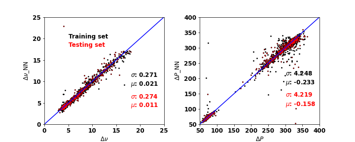
After estimating asteroseismic parameters for training and testing samples, we compare our frequency spacing and period spacing ($\Delta\nu_{\rm NN}$ and $\Delta P_{\rm NN}$) with these provided by Vrard et al. (2016) for testing stars, as shown in Fig. 1. We can find that our $\Delta\nu_{\rm NN}$ and $\Delta P_{\rm NN}$ match well with these of Vrard et al. (2016). Our neural network could derive precise frequency spacing and period spacing from LAMOST spectra.

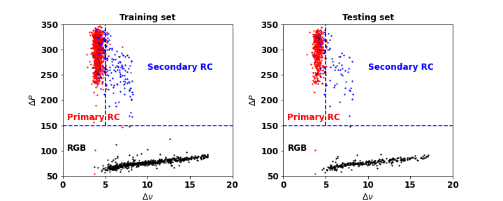
The $\Delta P$ of RC and RGB stars are very different, they are $\sim$ 300s and $\sim$ 70s, respectively (Bedding et al. 2011; Ting et al. 2018). Fig. 2 shows the stellar distributions on the plane of $\Delta\nu$ and $\Delta P$ derived by neural network method for training and testing sample. The plots clearly show that a gap of $\Delta P$ between the RGB and RC stellar populations is visible for both training and testing samples. It illustrates that the spectroscopically estimated frequency spacing and period spacing ($\Delta\nu$ and $\Delta P$ ) using our neural network method, especially $\Delta P$, could allow one to separate the RC stars from the RGB stars. Here we identify giant stars with $\Delta P>150$ s as RCs, and giant stars with $\Delta P\leq 150$ s as red giant stars.

Fig. 2 also suggests that it is also possible to classify primary and secondary RC stars using the spectroscopically estimated frequency spacing and period spacing. RC stars with $\Delta\nu>6\mu$Hz can be classified as secondary RC stars (Yang et al. 2012; Ting et al. 2018). To separate the primary RCs from the secondary RCs, we select $\Delta P>150$ s and $\Delta\nu>5\mu$Hz as secondary RCs, $\Delta P>150$ s and $\Delta\nu\leq 5\mu$Hz as primary RCs.

The completeness of RGB, primary RC, and secondary RC are respectively 99.2%(280/282), 96.8%(485/501), and 62%(49/79) examined by the testing set. The purity of RGB, primary RC, and secondary RC are respectively 98.9% (280/283), 94.2% (485/515), and 79% (49/62) examined again by the testing set.

We adopt the constructed neural network model to $\sim$1.3 million LAMOST spectra collected by LAMOST DR8 of giant stars to estimate their spectroscopic frequency spacing and period spacing. With the aforementioned criteria of separating RGBs, primary RCs and secondary RCs, 937,082, 244,458, and 167,105 spectra for 696,680 unique RGBs, 180,436 unique primary RCs and 120,907 unique secondary RCs with spectral SNRs $>10$ are found. For a star with multiple observed spectra, the classification, mass and age derived by the spectrum with the highest spectral SNR are suggested.

Figure 1: The comparisons of $\Delta\nu$ and $\Delta P$ provided by Vrard et al. (2016) ($X$-axis) using Kepler data and that derived by neural network model ($Y$-axis) for $1,800$ training (black dots) and $862$ testing stars (red dots). The values of the mean and standard deviation of the differences are labelled in the bottom-right corner of each panel.

Figure 2: The stellar distributions on the plane of $\Delta\nu$-$\Delta P$ derived by neural network method for 1,800 training (left panel) and 862 testing stars (right panel). The black, red and blue dots show the 826 RGBs, 1,599 primary RCs and 237 secondary RCs classified by Vrard et al. (2016) using Kepler data, respectively. The blue dashed line ($\Delta P=150$ s) is plotted to separate RGBs and RCs. The black dashed line ($\Delta\nu=5\mu$Hz) is plotted to separate primary RCs and secondary RCs.

4 Ages and masses of RGBs and RCs

In this Section, we estimate the masses and ages of our RGBs, primary RCs and secondary RCs selected from the LAMOST low-resolution spectroscopic survey. Doing so, we first estimate the masses and ages using the respective asteroseismic information and isochrone fitting method, for LAMOST-Kepler giant stars. Then we estimate masses and ages for all LAMOST DR8 giant stars, using the neural network method by taking the LAMOST-Kepler giant stars as the training set. For both RGBs and RCs, we build up two different neural network models to estimate ages and masses, respectively.

4.1 Ages and masses of LAMOST-Kepler training and testing stars

Masses of RGBs and RCs can be accurately measured from the asteroseismic information achieved by Kepler mission. We cross-match our RGB and RC samples to the Kepler sample with accurate asteroseismic parameters measured by Yu et al. (2018), using light curves of stars provided by the Kepler mission. In total, 3,220 and 3,276 common RGBs and RCs are found with both high-quality spectra (SNR$>$50), well-derived spectroscopic and precise asteroseismic parameters.

For these RGB and RC common stars, we determine their asteroseismic masses using modified scaling relations,

$$\frac{M}{M_{\odot}}=(\frac{\Delta\nu}{f_{\Delta\nu}\Delta\nu_{\odot}})^{-4}(\frac{\nu_{\rm max}}{\nu_{\rm max,\odot}})^{3}(\frac{T_{\rm eff}}{T_{\rm eff,\odot}})^{3/2},$$ (2)

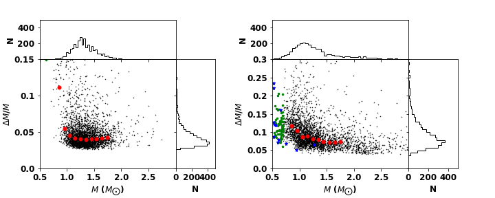
Here the Solar values of $T_{\rm eff,\odot}$, $\nu_{\rm max,\odot}$ and $\Delta\nu_{\odot}$ are 5777 K, 3090 $\mu$Hz and 135.1 $\mu$Hz (Huber et al. 2011), respectively. Where $f_{\Delta\nu}$, the correction factor can be obtained for all stars using the publicly available code $Asfgrid^{11}$ provided by Sharma et al. (2016). With this modified scaling relation, the masses of these 3,220 and 3,276 RGB and RC common stars are derived with precise $\Delta\nu$ and $\nu_{\rm max}$ provided by Yu et al. (2018) and effective temperature $T_{\rm eff}$ taken from Wang et al. (2022). Fig. 3 shows the masses distributions estimated from the asteroseismic and spectroscopic stellar atmospheric parameters, as well as their associated uncertainties. The plot clearly shows that the typical uncertainties of masses of RGBs and RCs are respectively 4.1 and 8.4 per cent.

There are several stars with a mass lower than 0.7 $\,M_{\odot}$ as shown in Fig. 3, especially for RCs. Some of these stars may be post-mass-transfer helium-burning stars (Li et al. 2022b), which may be in binary systems, suffered a mass-transfer history with a mass-loss of about 0.1–0.2 $\,M_{\odot}$. We make a crossmatch to the list of post-mass-transfer helium-burning red giants provided by Li et al. (2022b) and find twelve common stars, nine of them are stars with $M<0.7\,M_{\odot}$. In the current work, we did not consider such an extreme mass-loss case and thus the readers should be careful of the parameters of a star with a mass smaller than 0.7 $M_{\odot}$.

Figure 3: Distributions of 3,220 LAMOST-Kpler common RGBs (left panels) and 3,276 LAMOST-Kpler common RCs (right panels) on the $M$–$\Delta M/M$ plane. $M$ and $\Delta M$ are the estimated masses and their associated uncertainties. The red dot presents the median values in each mass bin with a bin size of 0.1 $M_{\odot}$. Green dots are stars with $M<0.7\,M_{\odot}$. Blue stars show the post-mass-transfer helium-burning stars identified by Li et al. (2022b). Distributions of masses and their associated uncertainties are over-plotted using histograms.

We further estimate the ages of these common stars based on the stellar isochrone fitting method using the aforementioned estimated masses and the effective temperatures, metallicities and surface gravities provided by Wang et al. (2022). Similar to that of Huang et al. (2020), we adopt the PARSEC isochrones calculated with a mass-loss parameter $\eta_{\rm Reimers}=0.2$ (Bressan et al. 2012) as the stellar evolution tracks. Here, we adopt one Bayesian approach similar to Xiang et al. (2017) and Huang et al. (2020) when doing isochrone fitting. The mass $M$, effective temperatures $T_{\rm eff}$, metallicity [M/H] and surface gravity $\log g$ are the input constraints.

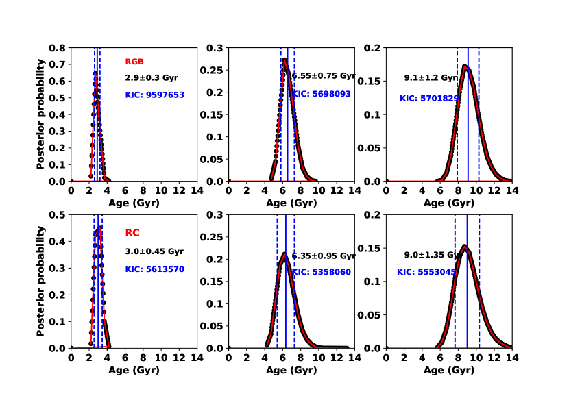
The posterior probability distributions as a function of age for three stars of typical ages for both RGB and RC stars are shown in Fig. 4. As shown in Fig. 4, we can find that the age distributions show prominent peaks, which suggest that the resultant ages are well constrained, especially thanks to the precise mass estimates from asteroseismology information. Fig. 5 shows the distributions of ages, as well as the uncertainties, of RGBs and RCs, estimated using the isochrone fitting method. Both the RGB and RC samples cover a whole range of possible ages of stars, from close to zero to 13 Gyr (close to the universe age). The typical age uncertainties of RGB and RC stars are 14 and 23 per cent, respectively. There are only a small fraction stars that have age uncertainties larger than 40 per cent. Larger age uncertainties of RCs compared to RGBs are the consequence of larger mass uncertainties of RCs. It is noted that the relationship between age and its associated uncertainty of RGBs is opposite to that of RCs at $\tau<8$ Gyr, which may be the consequence of the larger variations of mass uncertainty of RCs compared to that of RGBs at $1.0<M<1.5\,M_{\odot}$. The mass uncertainty decrease 1.7% and 0.02% when mass decrease from 1.55 $\,M_{\odot}$ ($\tau\sim 2.0$ Gyr) to 1.05 $\,M_{\odot}$ ($\tau\sim 9.0$ Gyr) for RCs and RGBs, respectively. Large mass uncertainties produce large age uncertainties ($\Delta\tau$), thus older RGBs and RCs have respectively smaller and larger relative age uncertainties ($\Delta\tau/\tau$).

Figure 4: The posterior probability distributions as a function of age for three stars of typical ages for both RGB (top panels) and RC (bottom panels) stars. The blue solid lines denote the median values of the stellar ages. The blue dashed lines show the standard deviations of the stellar ages. The KIC number of the six stars are given here.

Figure 5: Distributions of 3,220 LAMOST-Kepler common RGBs (left panels) and 3,276 LAMOST-Kepler common RCs (right panels) on the $\tau$–$\Delta\tau/\tau$ plane. $\tau$ and $\Delta\tau$ are the estimated ages using the isochrone fitting method and their associated uncertainties. The red dot presents the median value in each age bin with a bin size of 1.0 Gyr. Green dots are stars with $M<0.7\,M_{\odot}$. Blue stars show stars the post-mass-transfer helium-burning stars identified by Li et al. (2022b). Distributions of ages and their associated uncertainties are over-plotted using histograms.

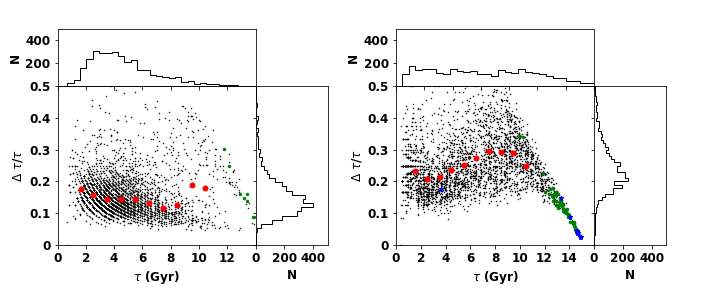
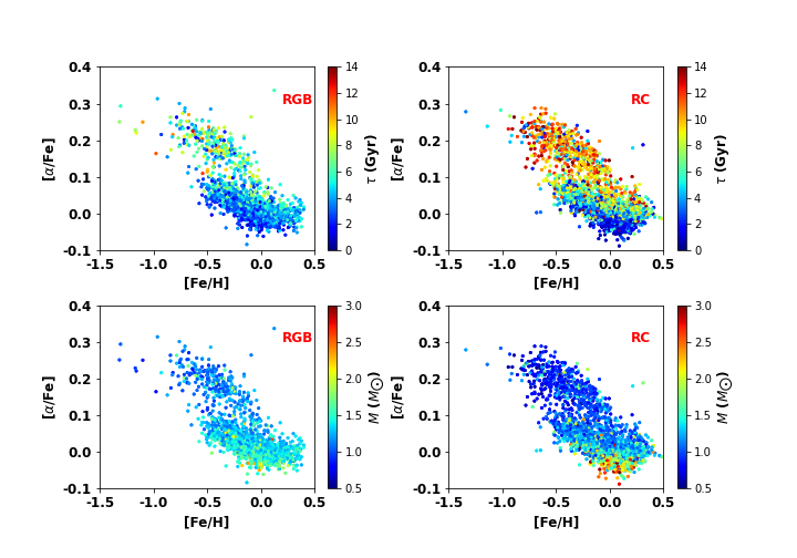
After estimating the masses and ages of these 3,103 and 3,114 RGB and RC common stars, we divide both RGB and RC common stars into two sub-samples, a training and a testing sub-sample. The training sample of RGB and RC contains 1,493 and 2,499 stars, respectively. Other 1,610 and 615 RGB and RC stars form the testing samples. When selecting training stars, the number of training stars in each age bin is the same as each other as much as possible. As shown in Fig. 5, the RGB sample contains fewer old stars as compared to the RC sample. This is the same for the training set. Fig. 6 shows the distributions of the RGB, RC training samples and testing samples on the [M/H]–[$\alpha$/Fe] plane, colour-coded by mass and age.

Figure 6: Distributions of LAMOST-Kepler 1,493 training RGB stars (left panels) and 2,499 training RC stars (right panels) on the [Fe/H]–[$\alpha$/Fe] plane, colour-coded by stellar age (top panels) and mass (bottom panels). Here the values of [Fe/H] and [$\alpha$/Fe] come from the value-added catalogue of LAMOST DR8 (Wang et al. 2022).

4.2 Age and mass determinations of RGB and RC stars in LAMOST DR8

After building up the training and testing stars with accurate masses and ages, we derive masses and ages of RGB and RC stars from the LAMOST DR8 spectra, using the neural network method, which is detailed described in Section 3.1. The aforementioned RGB and RC training stars are adopted as training samples. After pre-processing the LAMOST spectra (same as that of Wang et al. (2022)) of all the training and testing stars, we build up the model to construct the relation between the pre-processed LAMOST spectra and mass/age for RGBs and RCs. Our neural network models to estimate masses and ages also contain three layers, the total number of neurons for the first, second, and third layers are respectively 512, 256, and 64, which is the same as the neural network models to estimate asteroseismic parameters in Section 3.

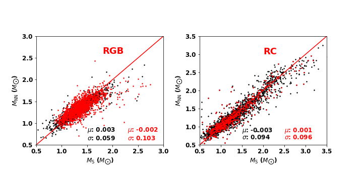
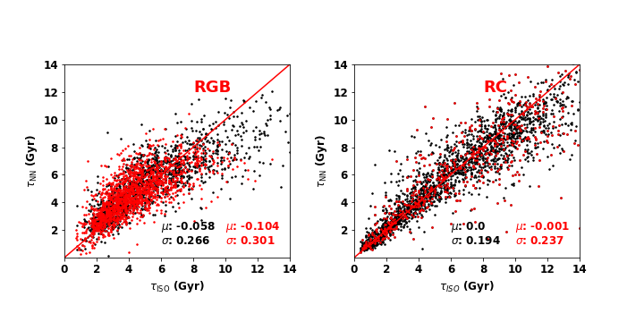
Fig. 7 shows the comparison of mass estimated with scaling relation ($M_{S}$) in Section 4.1 and mass derived by neural network model ($M_{\rm NN}$) using LAMOST spectra for testing RGB and RC stars. We can find that $M_{\rm NN}$ match well with $M_{S}$ for individual stars. The systematic uncertainties are very small, the standard deviations of estimated mass are 10 per cent and 9.6 per cent for RGBs and RCs, respectively. Fig. 8 shows the comparison of age estimated with the isochrone fitting method ($\tau_{\rm ISO}$) in Section 4.1 and age derived by neural network model ($\tau_{\rm NN}$) using LAMOST spectra for testing RGB and RC stars. We can find that the $\tau_{\rm NN}$ is consistent with the $\tau_{\rm ISO}$ for individual stars. The $\tau_{\rm NN}$ are overestimated about 10 per cent for RGB stars. The systematic uncertainties of $\tau_{NN}$ of RCs are very small. The standard deviations of estimated age are 30 per cent and 24 per cent for RGBs and RCs, respectively. Figs. 7 or 8 also show the comparisons between $M_{\rm NN}$ and $M_{S}$ or $\tau_{\rm NN}$ and $\tau_{\rm ISO}$ for training stars. The $M_{\rm NN}$ ($\tau_{\rm NN}$) is well in agreement with $M_{S}$ ($\tau_{\rm ISO}$). The standard deviations of estimated mass are respectively 5.9 per cent and 9.4 per cent for RGB and RC training stars. For age estimates of RGB and RC training stars, the standard deviations are 26.6 per cent and 19.4 per cent, respectively. In summary, our neural networks could derive precise mass and age for RGB and RC stars from LAMOST spectra.

Finally, we adopt our neural network models to 937,082, 244,458, and 167,105 RGB, primary RC and secondary RC stellar spectra and derive their spectroscopic masses and ages.

Figure 7: The comparisons of mass estimated with scaling relation ($M_{\rm S}$) in Section 4.1 and mass derived by neural network model ($M_{\rm NN}$) using LAMOST spectra for LAMOST-Kepler RGB (left panel) and RC (right panel) stars testing sample (red dots; 1,610 RGBs, 615 RCs) and training sample (black dots; 1,493 RGBs, 2,499 RCs). The $\mu$ and $\sigma$ are the mean and standard deviations of $(M_{\rm S}-M_{\rm NN})$/$M_{\rm S}$, as marked in the bottom-right corner of each panel.

Figure 8: The comparisons of age estimated with isochrone fitting ($\tau_{\rm ISO}$) in Section 4.1 and age derived by neural network model ($\tau_{\rm NN}$) using LAMOST spectra for LAMOST-Kepler 3,103 RGB (left panel) and RC (right panel) stars in the testing sample (red dots; 1,610 RGBs, 615 RCs) and training sample (black dots; 1,493 RGBs, 2,499 RCs). The $\mu$ and $\sigma$ are the mean and standard deviations of $(\tau_{\rm ISO}-\tau_{\rm NN})$/$\tau_{\rm ISO}$, as marked in the bottom-right corner of each panel.

5 Validation of the spectroscopic masses and ages of RGBs and RCs

In this section, we first examine the uncertainties of the masses and ages of RGBs and RCs using the neural network method through internal comparisons. Secondly, through external comparisons, we further examine the uncertainties, including the systematic biases, of masses and ages.

5.1 The uncertainties of estimated masses and ages of RGBs and RCs

The uncertainties of estimated masses and ages depend on the spectral noise (random uncertainties) and method uncertainties.

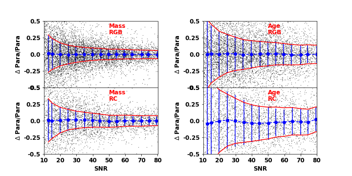
As discussed in Huang et al. (2020) and Wang et al. (2022), the random uncertainties of masses and ages are estimated by comparing results derived from duplicate observations of similar spectral SNRs (differed by less than 10 per cent) collected during different nights. The relative residuals of mass and age estimate (after divided by $\sqrt{2}$) along with mean spectral SNRs are shown in Fig. 9. To properly obtain random uncertainties of age and mass, we fit the relative residuals with the equation similar to Huang et al. (2020):

$$\sigma_{r}=a+\frac{c}{(\rm SNR)^{\emph{b}}},$$ (3)

where $\sigma_{r}$ represents the random uncertainty. Besides the random uncertainties, method uncertainties ($\sigma_{m}$) are also considered when we estimate the uncertainties of stellar parameters. The final uncertainties are given by $\sqrt{\sigma_{r}^{2}+\sigma_{m}^{2}}$. The method uncertainties are provided by the relative residuals between our estimated results and the asteroseismic results of the training sample. For the age and mass of RGB stars, the method uncertainties are 26.6 and 5.9 per cent as shown in Figs. 7 and 8, respectively. The method uncertainties of age and mass are 19.4 and 9.4 per cent for RC stars as shown in Figs. 7 and 8, respectively.

Figure 9: Relative internal residuals of estimated masses (left panels) and ages (right panels) using neural network method given by duplicate observations of similar spectral SNRs for LAMOST RGB (top panels) and RC (bottom panels) stars. Black dots are the differences of duplicate observations of SNR differences smaller than 10 %. Blue dots and error bars represent the median values and standard deviations (after divided by $\sqrt{2}$) of the relative residuals in the individual spectral SNR bin. Red lines indicate fits of the standard deviations as a function of spectral SNRs.

5.2 The ages of members of open clusters

Stars in the open cluster are believed to form almost simultaneously from a single gas cloud, thus they have almost the same age, metallicity, distance and kinematics. Open cluster is a good test bed to check the accuracy of ages. Zhong et al. (2020a) and Zhong et al. (2020b) provide 8,811 cluster members of 295 clusters observed by LAMOST, who cross-match the open cluster catalogue and the member stars provided by Cantat-Gaudin et al. (2018) with LAMOST DR5. Amongst these clusters, open clusters with a wide age range (1–10 Gyr) are carefully selected for checking our age estimates. As shown in Fig. 10, we can find that our ages of open clusters are consistent with these of literature for both RGB and RC stars from the young part ($\sim$ 2 Gyr) to the old part ($\sim 10$ Gyr). Table. 1 present our age estimates and literature age values.

Figure 10: Comparisons of our estimated ages ($\tau_{\rm NN}$) of open clusters with literature values ($\tau_{\rm LIT}$) for LAMOST RGBs (left panel) and RCs (right panel).

Table 1: Age values of open clusters estimated using our neural network and ages of literature values for both LAMOST RGB and RC stars. The numbers of RGB and RC cluster members are also presented.

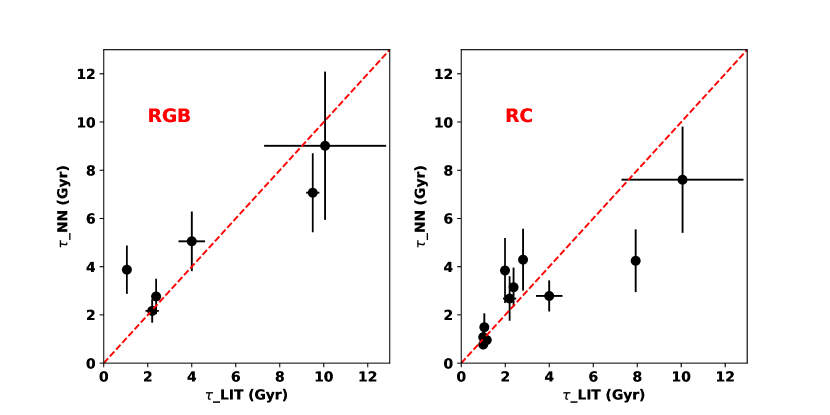
Cluster	LIT age (Gyr)	age of RGB (Gyr)	number of RGB	age of RC (Gyr)	number of RC	References *
NGC 6811	1.00$\pm$0.10	–	0	0.76$\pm$0.19	6	1, 2
NGC 2420	2.20$\pm$0.30	2.16$\pm$0.48	1	2.67$\pm$0.92	4	3
NGC 6819	2.38$\pm$0.22	2.76$\pm$0.73	6	3.14$\pm$0.81	14	4, 5
NGC 2682	4.00$\pm$0.60	5.05$\pm$1.23	6	2.78$\pm$0.64	2	6
NGC 6791	9.50$\pm$0.30	7.06$\pm$1.61	2	–	–	7
Berkeley 17	10.06$\pm$2.77	9.01$\pm$3.07	2	7.6$\pm$2.04	2	3, 8
Berkeley 21	1.99	–	0	3.84$\pm$1.34	2	9–11
Berkeley 39	7.93	–	0	4.24$\pm$1.29	2	9–11
Berkeley 78	2.81	–	0	4.29$\pm$1.28	2	9–11
Czernik 27	1.16	–	0	0.96$\pm$0.26	2	9–11
FSR 0850	1.0$\pm$0.05	–	0	1.07$\pm$0.38	2	9–11
NGC 1245	1.05	3.87$\pm$1.00	5	1.49$\pm$0.56	12	9–11

• Notes. * References: (1) Sandquist et al. (2016); (2) Molenda-Żakowicz et al. (2014); (3) Salaris et al. (2004); (4) Anthony-Twarog et al. (2014); (5) Brewer et al. (2016); (6) Stello et al. (2016); (7) An et al. (2015); (8) Bragaglia et al. (2006); (9) Zhong et al. (2020b); (10) Kharchenko et al. (2013); (11) Bossini et al. (2019).

5.3 Comparison of masses and ages of RGB and RC stars with previous results

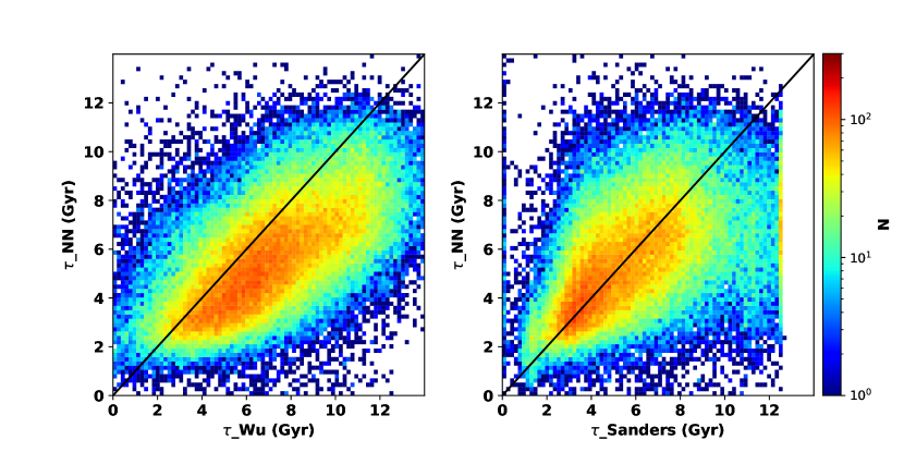
A catalogue containing accurate stellar ages for $\sim$0.64 million RGB stars targeted by the LAMOST DR4 has been provided by Wu et al. (2019). Sanders & Das (2018) has determined distances, and ages for $\sim$3 million stars with astrometric information from Gaia DR2 and spectroscopic parameters from massive spectroscopic surveys: including the APOGEE, Gaia-ESO, GALAH, LAMOST, RAVE, and SEGUE surveys. We cross-match our catalogue with their catalogues and obtain $\sim$ 97,000 and 83,000 common RGB stars (SNR$\geq$50, 2.0 $<\log g<$ 3.2 dex, 4000 $<T_{\rm eff}<$ 5500 K) with the catalogue of Wu et al. (2019) and Sanders & Das (2018), respectively. The comparisons are shown in Fig. 11. Generally, our ages are younger than those estimated by Wu et al. (2019). In particular, for the old parts, our ages are younger than the ages of Wu et al. (2019) with 2–3 Gyr. This is mainly the different choices of isochrone database between this work and Wu et al. (2019), who adopt the isochrones from PARSEC and Yonsei–Yale ($\rm Y^{2}$; Demarque et al. 2004), respectively. The lack of old (low mass: $M<1.0\,M_{\odot}$) RGB training stars in this work may also cause our relatively younger age estimates. Our estimated ages could agree well with these estimated by Sanders & Das (2018).

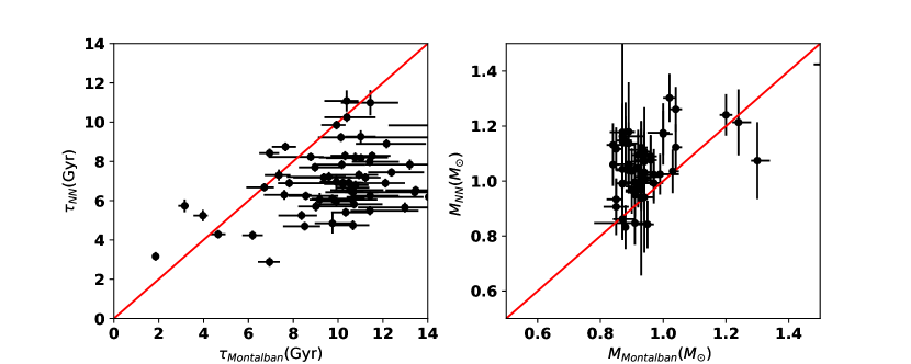
Montalbán et al. (2021) has provided precise stellar ages ($\sim 11$%) and masses for 95 RGBs observed by the Kepler space mission by combining the asteroseismology with kinematics and chemical abundances of stars. There are 62 common stars between our catalogue and their list. As shown in Fig. 12, ages of old stars with $\tau>8$ Gyr are underestimated by 2–3 Gyr compared to the results of Montalbán et al. (2021), because masses of these stars are overestimated by $\sim 0.1M_{\odot}$. Montalbán et al. (2021) estimate the masses adopting the individual frequencies of radial modes as observational constraints, which may provide more accurate masses (Lebreton & Goupil 2014; Miglio et al. 2017; Rendle et al. 2019; Montalbán et al. 2021). Building up a training sample containing enough RGBs with accurate age and mass estimates adopting individual frequencies as observational constraints may dramatically improve the determination of age and mass for RGBs using machine learning methods. A potential challenge is the lack of precise individual frequencies for a larger sample size of red giant stars ($\sim$2000–6000 stars). Yet this is out of the topic in this paper.

Figure 11: Comparisons of our estimated ages with these provided by Wu et al. (2019) (left panel) and Sanders & Das (2018) (right panel) for 97,112 and 83,199 common RGB stars with $\rm SNRs>50$, respectively.

Figure 12: Comparisons of our estimated ages and masses with these provided by Montalbán et al. (2021) for 62 common RGB stars.

The precise distances, masses, ages and 3D velocities for $\sim$140,000 primary RCs selected from the LAMOST have been determined by our former effort (Huang et al. 2020). The catalogue of Sanders & Das (2018) also contain a lot of RC stars with age estimates. Our catalogue has $\sim$ 52,000 and 72,000 RC stars (SNR$\geq$50) in common with the catalogue of Huang et al. (2020) and Sanders & Das (2018). Fig. 13 shows the comparisons between ages in this work and the ages of Huang et al. (2020) and Sanders & Das (2018) for RC stars. Our ages are consistent very well with these of Huang et al. (2020). The ages in this work are generally consistent with these of Sanders & Das (2018), although a mild offset of 2–3 Gyr (this work minus Sanders & Das (2018)) is detected.

Figure 13: Comparisons of our estimated ages with these provided by Huang et al. (2020) (left panel) and Sanders & Das (2018) (right panel) for 42,969 and 52,944 common RC stars with $\rm SNRs>50$, respectively.

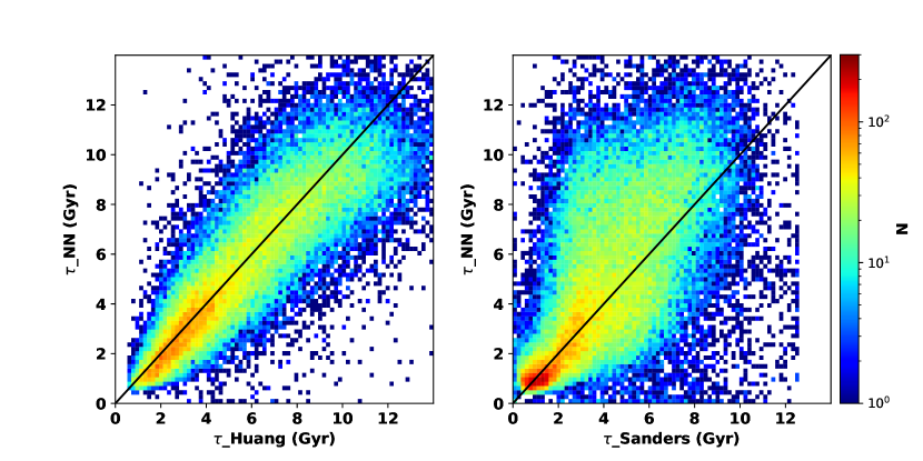
In summary, the uncertainties of ages and masses of RC stars are smaller than 25 and 10 per cent for stars with spectral SNR $>50$ through the internal comparisons, respectively. For RGB stars with spectral SNR $>50$, the uncertainties of ages and masses are respectively smaller than 20 and 8 per cent. The systematic uncertainties of our age estimates are very small for both RGB and RC stars, by comparing the age derived in this work to the literatures for open cluster member stars. Our age estimations match well with these of Sanders & Das (2018) for RGB stars and these of Huang et al. (2020) for RC stars.

6 Properties of the LAMOST RGB and RC samples

Besides the accurate masses and ages estimated here, the stellar atmospheric parameters ($T_{\rm eff}$, $\log\,g$ and [Fe/H]), chemical element abundance ratios ([M/H], [$\alpha$/M], [C/Fe] and [N/Fe]) and 14 bands absolute magnitudes ($M_{G},M_{Bp},M_{Rp}$ of Gaia bands, $M_{J},M_{H},M_{Ks}$ of 2MASS bands, $M_{W1},M_{W2}$ of WISE bands, $M_{B},M_{V},M_{r_{A}}$ of APASS bands and $M_{g},M_{r},M_{i}$ of SDSS bands) and photometric distances are also provided, which are taken from the value-added catalogue of LAMOST DR8 built up by Wang et al. (2022). Thus, we could study the spatial coverage, and age distributions on the $R$–$Z$ plane and on the [Fe/H]–[$\alpha$/Fe] plane of our RGB, primary RC and secondary RC samples.

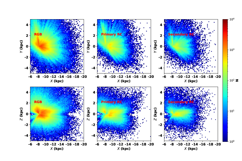
Fig. 14 shows the stellar number density distributions of our RGB, primary RC and secondary RC stellar samples on the $X$–$Y$ and $X$–$Z$ planes, which cover a large volume of the Milky Way ($5<R<20$ kpc and $|Z|<5$ kpc). One can use it to probe the structural, chemical, and kinematic properties of both the Galactic thin, thick discs and halo combining the proper motions provided by Gaia DR3 (Gaia Collaboration et al. 2022; Babusiaux et al. 2022).

Figure 14: Stellar number density distributions of the 520,073 unique LAMOST RGB (left panels), 154,587 unique primary RC (middle panels) and 66,395 unique secondary RC (right panels) stars with spectral $\rm SNRs>20$ on the $X$–$Y$ (top panels) and $X$–$Z$ (bottom panels) planes in Galactic Cartesian coordinates.

Figure 15: The median age distributions of the 259,372 unique LAMOST RGB (left panels), 92,795 unique primary RC (middle panels) and 2,8104 unique secondary RC (right panels) stars with spectral $\rm SNRs>50$ on the $R$–$Z$ plane.

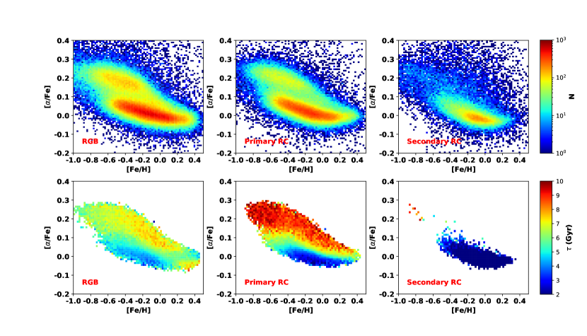
The age distributions of RGB, primary RC and secondary RC stars on the $R$–$Z$ plane are presented in Fig. 15. From this figure, we can see that there are negative age gradients in the radial direction and positive age gradients in the vertical direction for both RGB and primary RC stars, which are reported in a series of previous studies (e.g., Martig et al. 2016b; Casagrande et al. 2016). For secondary RCs, there are positive age gradients in the vertical direction. Flat or slightly positive radial age gradients are found for secondary RCs, which may be meaningless considering the small mean age coverage (from $\sim$ 1.1 Gyr at $R\sim 9$ kpc to 1.5 Gyr at $R\sim$12 kpc) and large age uncertainties at youngest part. The strong flaring of young Galactic disc (young stellar populations extended to higher heights from the Galactic plane with $R$ increasing) is clearly seen in the age distributions of RGB and primary RC stars. Similar results are also noted by Xiang et al. (2017), Wu et al. (2019) and Huang et al. (2020).

Fig.16 shows the stellar number density and mean age distributions on the [Fe/H]–[$\alpha$/Fe] plane for the RGB, primary RC and secondary RC stars. The stellar number density distributions of RGB and primary RC stars suggest that the RGB and primary RC stellar populations could be clearly distinguished into two individual sequences, the high-$\alpha$ and low-$\alpha$ sequences. The high- and low-$\alpha$ sequences are associated with the so-called chemically thick and thin discs. For primary RC stellar populations, the mean age of high- and low-$\alpha$ sequence are $\sim$ 8 Gyr and $\sim 2.5$ Gyr, respectively. The high-$\alpha$ sequence is older than the low-$\alpha$ sequence. The results are consistent with previous findings for the solar neighbourhood using high-resolution spectroscopy (Bensby et al. 2003; Haywood 2008; Haywood et al. 2013; Hayden et al. 2015) and results using a large sample of stars with ages derived from the LAMOST low-resolution spectra (Xiang et al. 2017; Wu et al. 2019; Huang et al. 2020). For RGB stellar populations, the age of high- and low-$\alpha$ sequences are $\sim 6$ Gyr and $\sim 3$ Gyr, respectively. The high-$\alpha$ sequence is older than the low-$\alpha$ sequence with a smaller age difference as compared to that of primary RC stellar populations. For RGB stellar populations, the eldest stellar populations are located in the transition region of high- and low-$\alpha$ sequences. Almost all of secondary RC stars are thin disc stars, because they are massive young stars.

For both RGB and primary RC stellar populations, there are some stars with metallicity higher than 0.2 dex and older than low-$\alpha$ sequence. Some of these stars are the so-called “old yet metal-rich” stars ($6<\tau<8$ Gyr, $[\rm Fe/H]>0.2$ dex, $-0.05<[\alpha/\rm Fe]<0.05$ dex). It has been suggested that these “old yet metal-rich” stars may come from the inner disc through radial migration processes (Xiang et al. 2015; Wang et al. 2019; Feuillet et al. 2018, 2019; Hasselquist et al. 2019; Boeche et al. 2013; Chen et al. 2019) . Old and metal-rich stars in the inner disc will move outward through the radial migration process and produce these “old yet metal-rich” stars.

Figure 16: The stellar number density (top panels) and mean age (bottom panels) distributions on the [Fe/H]–[$\alpha$/Fe] plane for the 259,372 unique LAMOST RGB (left panels), 92,795 unique primary RC (middle panels) and 2,8104 unique secondary RC (right panels) stars with spectral $\rm SNRs>50$.

7 Summary

In the current work, we build up a catalogue of masses and ages for 937,082, 244,458, and 167,105 RGBs, primary RCs and secondary RCs selected from LAMOST DR8 low-resolution stellar spectra of spectral SNR $>$ 10. Amongst them, 696,680 RGBs, 180,436 primary RCs, and 120,907 secondary RCs are unique stars. The RGBs, primary RCs and secondary RCs are identified with the large frequency spacing ($\Delta\nu$) and period spacing ($\Delta P$) estimated using a neural network method. The contaminations of RGB stars from RC stars and contaminations of RCs from RGBs are both about 1 per cent for stars with spectral SNR $>$ 20.

Using the relations of stellar spectra and the masses and ages built up by neural network method using the RGB and RC stars in the LAMOST-Kepler fields that have accurate asteroseismic mass and age measurements as training samples, the masses and ages of all LAMOST RGB and RC stars are estimated. The typical uncertainties of estimated masses and ages, as examined by the testing sample, are respectively 10% and 30% for RGB stars, and respectively 9% and 24% for RC stars.

The RGB and RC stellar populations cover a large volume of the Milky Way ($5<R<20$ kpc and $|Z|<5$ kpc). The stellar atmospheric parameters, chemical element abundances, 14 bands absolute magnitudes and photometric distances are also given here. One can use it to probe the structural, chemical, and kinematic properties of both the Galactic thin, thick discs and halo combining the proper motions provided by Gaia DR3. The catalogue is available at the CDS and the LAMOST official website .