Near-Infrared Spectroscopy of Dense Ejecta Knots in the Outer Eastern Area of the Cassiopeia A Supernova Remnant

Abstract

The Cassiopeia A supernova remnant has a complex structure, manifesting the multidimensional nature of core-collapse supernova explosions. To further understand this, we carried out near-infrared multi-object spectroscopy on the ejecta knots located in the ”northeastern (NE) jet” and the “Fe K plume” regions, which are two distinct features in the outer eastern area of the remnant. Our study reveals that the knots exhibit varying ratios of [S II] 1.03 µm, [P II] 1.189 µm, and [Fe II] 1.257 µm lines depending on their locations within the remnant, suggesting regional differences in elemental composition. Notably, the knots in the NE jet are mostly ‘S-rich’ with weak or no [P II] lines, implying that they originated below the explosive Ne burning layer, consistent with the results of previous studies. We detected no ejecta knots exhibiting only [Fe II] lines in the NE jet area that are expected in the jet-driven SN explosion model. Instead, we discovered a dozen ‘Fe-rich’ knots in the Fe K plume area. We propose that they are dense knots produced by a complete Si burning with $\alpha$-rich freezeout in the innermost region of the progenitor and ejected with the diffuse X-ray emitting Fe ejecta but decoupled after crossing the reverse shock. In addition to these metal-rich ejecta knots, several knots emitting only He I 1.083 µm lines were detected, and their origin remains unclear. We also detected three extended H emission features of circumstellar or interstellar origin in this area and discuss its association with the supernova remnant.

1 Introduction

The core-collapse supernova (SN) explosion is one of the outstanding problems in modern astrophysics. It is generally agreed that, for the majority of core-collapse SNe, the explosion is initiated by a core-bounce shock which becomes stalled but is revived by neutrino heating. Modern state-of-the-art three-dimensional simulations show that this neutrino-driven SN explosion is basically multi-dimensional, facilitated by turbulent convection and hydrodynamic instabilities (e.g., see Janka, 2017; Burrows & Vartanyan, 2021). The non-uniform, inhomogeneous, and radially mixed/overturned distribution of metal-rich ejecta in SNe and young SN remnants (SNRs) provide strong observational evidence for it.

Cassiopeia A (Cas A) is a unique SNR where we can see the details of the spatial and velocity distribution of SN ejecta. It is young ($\sim 350$ yrs; Thorstensen et al., 2001; Fesen et al., 2006) and nearby (3.4 kpc; Reed et al., 1995; Alarie et al., 2014). It is a remnant of SN Type IIb with a probable progenitor mass of 15–$25~{}M_{\sun}$ (Young et al. 2006; Krause et al. 2008; see also Koo & Park 2017 and references therein). The remnant is shell-type and has a basic appearance of a small, clumpy bright ring surrounded by a limb-brightened faint plateau. The bright ring has a radius of $1\farcm 7$ (1.7 pc) and is mainly composed of C and O burning ejecta material heated by reverse shock. The faint plateau extends to $2\farcm 6$ (2.5 pc), and its outer boundary defines the current position of the SN blastwave.

In detail, Cas A has a quite complex structure, manifesting the violent and asymmetric explosion. In the outer eastern area of the SNR, which is the area of primary interest in this study, there are two features distinguishable from the rest of the ejecta material. One is the “jet” structure in the northeastern (NE) area and the other is the Fe K-bright “plume” (hereafter the ‘NE jet’ and ‘Fe K plume’, respectively). The NE jet is a stream of compact optical knots confined into a narrow cone well outside the SN blast wave. It appears to have punched through the main ejecta shell, and the inferred ejection velocities is as large as 16,000 ${\rm km~{}s}^{-1}$, which is three times faster than the bulk of the ejecta in the main ejecta shell (Kamper & van den Bergh, 1976; Fesen & Gunderson, 1996; Fesen, 2001; Fesen & Milisavljevic, 2016). The optical knots show strong O, S, and Ar emission lines (van den Bergh, 1971; Fesen & Gunderson, 1996; Fesen, 2001; Fesen et al., 2006; Hammell & Fesen, 2008; Fesen & Milisavljevic, 2016). The NE jet structure was also observed by Chandra, which showed that the X-ray emitting jet material is rich in O-burning and incomplete Si-burning materials (Si, S, Ar, Ca), but poor in C/Ne-burning products (O, Ne, Mg) (e.g., Hughes et al., 2000; Hwang et al., 2004; Vink, 2004). The chemical composition of the jet material and the jet morphology suggest that the NE jet originated from a Si-S-Ar rich layer deep inside the progenitor and penetrated through the outer N- and He-rich envelope (Fesen, 2001; Fesen et al., 2006; Laming et al., 2006; Milisavljevic & Fesen, 2013). The other feature is the Fe K plume detected by Chandra and XMM-Newton in the eastern area (Willingale et al., 2002; Hwang & Laming, 2003; Hwang et al., 2004; Hwang & Laming, 2012; Tsuchioka et al., 2022). This plume of hot gas bright in Fe K line extends beyond the main ejecta shell bright in Si K and S K lines, and reaches the forward shock front. The velocity of the ejecta material in the outermost Fe K plume is $>4500$ ${\rm km~{}s}^{-1}$, much higher than that of Si/O-rich ejecta (Tsuchioka et al., 2022). The ejecta material in the Fe K plume has no S or Ar, and its Fe/Si abundance ratio is up to an order of magnitude higher than that expected in incomplete Si-burning layer, indicating that they originated from complete Si-burning process with $\alpha$-rich freezeout, where the burning products are almost exclusively ⁵⁶Fe (Thielemann et al. 1996; Hwang & Laming 2003, see also Sato et al. 2021). DeLaney et al. (2010) proposed a model for the Fe K plume where the Fe ejecta pushed through the Si layer as a “piston”, while Hwang & Laming (2003) and Milisavljevic & Fesen (2013) suggested that ⁵⁶Ni bubbles could produce plume-like structures in Fe K emission but the ionization age of the Fe K plume is inconsistent with a Ni bubble origin. We will explore the properties the NE jet and the Fe K plume in more detail in § 5 where we discuss the result of our work in this paper. Here we only emphasize that the distribution of Fe ejecta has not been fully explored: The Fe K plume revealed by X-ray observations is hot and ‘diffuse’ Fe-rich gas of density $\lower 2.15277pt\hbox{$\;\buildrel<\over{\sim}\;$}10$ cm^-3 (Hwang & Laming, 2003). Less hot ($\sim 10^{4}$ K) and presumably denser Fe-rich ejecta has not been explored. The presence or absence of Fe-rich ejecta material in the NE jet is also an important issue related to its origin, but it could not have been addressed in the previous optical studies (Fesen & Gunderson, 1996; Fesen, 2001; Fesen & Milisavljevic, 2016).

Recently, Koo et al. (2018) obtained a long-exposure ($\sim 10$ hr) image of Cas A by using the UKIRT 4-m telescope with a narrow band filter centered at [Fe II] 1.644 µm emission. The band includes [S I] 1.645 µm line, but it is faint and is non-negligible only for the unshocked ejecta in the inner area of the SNR (Koo et al., 2018; Raymond et al., 2018), so, in this paper, we refer the image as the “deep [Fe II] image”. The [Fe II] 1.644 µm line is one of the brightest near-infrared (NIR) lines in shocked gas, so it traces dense shocked material (e.g., Koo et al., 2016). The deep [Fe II] image revealed numerous knots in the outer eastern area beyond the main ejecta shell, the proper motion of which indicates that they are mostly SN ejecta material. The comparison with an HST WFC3/IR F098M image, which is dominated by sulfur lines (Hammell & Fesen, 2008; Fesen & Milisavljevic, 2016), showed that the majority of the knots in the image correspond to S-rich ejecta knots in optical studies. But a considerable fraction (21%) of the knots does not have optical counterparts, and the knots around the Fe K plume in the eastern area appear to have high Fe abundance (Koo et al., 2018). Hence, the study of these knots could provide new insights on the origin of the NE jet and the Fe K plume as well as the explosion dynamics of the Cas A SN.

In this work, we present the results of NIR spectroscopic observations of the knots in the deep [Fe II] image in the outer eastern area. In the NIR band (0.95–1.8 µm), in addition to the familiar He I 1.083 $\mu$m line and the forbidden lines of S II, S III, and Fe II, there is [P II] 1.089 $\mu$m (${}^{1}D_{2}\rightarrow$${}^{3}P_{2}$) line, which is the major NIR line of P II. Phosphorus (³¹P) is an uncommon element with cosmic abundance relative to H and Fe of $2.8\times 10^{-7}$ and $8.1\times 10^{-3}$ by number, respectively (Asplund et al., 2009). In young SNRs such as Cas A where we can observe SN ejecta, however, it could be a major element: Phosphorus is produced in hydrostatic neon-burning shells in the pre-SN stage and also in explosive carbon and neon-burning layers during SN explosion (Arnett, 1996; Woosley et al., 2002). Therefore, [P II] 1.089 $\mu$m line could be strong in some ejecta material of young SNRs and, together with the other strong lines of $\alpha$ elements (e.g., O, S, Fe), it can be used for the study of the SN explosion dynamics (Koo et al., 2013).

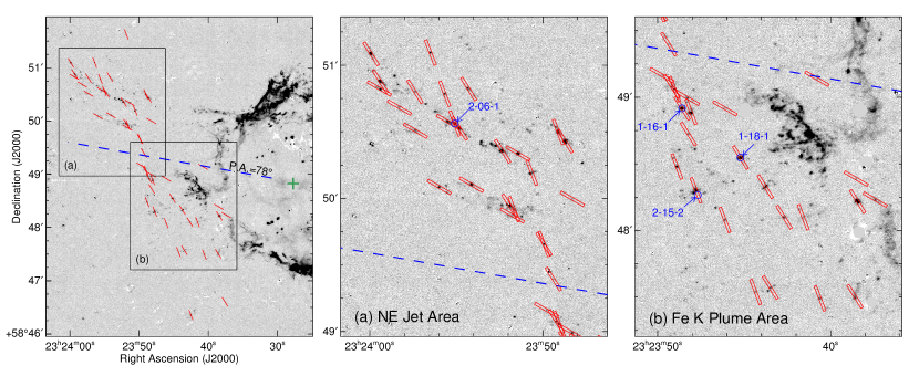
Figure 1: Finding charts for the slit positions. The red bars represent the locations of the 10″-long MOS slits in three masks. The background is the deep [Fe II] image taken in 2013 Sept. (Koo et al., 2018). The green cross marks the SN expansion center, ($23^{\rm h}23^{\rm m}27\fs 77\pm 0\fs 05$, $58\arcdeg 48\arcmin 49\farcs 4\pm 0\farcs 4$), obtained by Thorstensen et al. (2001). The blue dashed line represents the position angle of $78\arcdeg$ measured from north to east at the explosion center, which is used to divide the knots into two groups: (a) NE jet area knots and (b) Fe K plume area knots. Note that the slit positions are shifted to the 2013 epoch to match the background image (see the text for more detail). The 1-D spectra presented in Figure 7 correspond to the four ejecta knots labeled in blue on the figure.

The organization of the paper is as follows. In Section 2, we describe our NIR observations and explain the data reduction procedures. In Section 3, we explain how we obtain the spectral parameters of the knots for analysis. We identify individual knots in two-dimensional spectra and extract their one-dimensional spectra. We then derive the parameters of individual emission lines by performing single Gaussian fits. The derived fluxes are extinction corrected by using the Herschel SPIRE 250 $\mu$m data. In Section 4, we analyze the spectral properties of the ejecta knots. We find that there is significant variation in the ratios of bright lines among the knots in different areas. We classify the knots into different groups based on the bright line ratios and compare their spectral properties. We also search for optical counterparts of the knots and present the result. In Section 5, we discuss the origins of the knots and their connection to the explosion dynamics in Cas A. We focus on the knots in the NE jet region and those in the Fe K plume region. We also discuss the properties of the extended H emission features detected in the outer eastern area and its association with the Cassiopeia A SNR. Finally, in Section 6, we summarize the paper.

2 Observations and Data Reduction

We carried out NIR spectroscopic observations of the SN ejecta knots in the outer eastern area of Cas A in 2017 Sept. using MMT/Magellan Infrared Spectrograph (MMIRS) attached on MMT 6.5-m telescope. MMIRS is equipped with a HAWAII-2RG $2048\times 2048$ pixels HgCdTe detector with a pixel scale of $0\farcs 2012$ per pixel, which provides $6\farcm 9\times 6\farcm 9$ field-of-view for imaging observation (McLeod et al., 2012). In order to take $J$ and $H$-band spectra of the ejecta knots, we utilized the multi-object spectroscopy (MOS) mode with $J+zJ$ and $H3000+H$ (grism$+$filter) configurations that provide $J$-band (0.95–1.5µm) and $H$-band (1.50–1.80µm) spectra with a moderate spectral resolution.

In order to take NIR spectra of the ejecta knots, we carefully selected the bright knots in the outer eastern area from the deep [Fe II] image (Figure 1). Since the [Fe II] image was taken in 2013, we estimated the positions of the knots in the 2017 epoch assuming that they have been expanding freely from the explosion center during the age of Cas A. We prepared three MOS masks, each of which includes 20, 17, 15 MOS slits (Fig. 1). Each slit has a width of $0\farcs 8$ and a length of $10\arcsec$. This ‘moderate’ slit width provides the mean spectral resolving power of $\sim 8$ Å for $J$-band spectra and $\sim 7$ Å for $H$-band spectra, corresponding to $R\sim 1600$ at $1.26~{}\micron$ and $R\sim 2300$ at $1.64~{}\micron$, respectively. At all slit positions in Figure 1, we obtained $J$-band spectra. For the slits in MASK 1, we also took the $H$-band spectra. In order to subtract sky air-glow emission lines, we utilized ABBA observing sequence with dithering lengths of $+2\farcs 6$, $-2\farcs 0$, $-2\farcs 0$, $+2\farcs 6$. The single exposure time per frame was 300 sec, while the total effective exposure time per mask by the multiple frames were 40 min or 60 min for the $J$-band spectra, and 20 min for the $H$-band spectra. For the absolute flux calibration of the spectra, we also took the spectra of nearby A0V stars several times just before or after the target observations. The seeing during the observation was 0$\farcs$7–1$\farcs$2. The detailed observation log is listed in Table 1.

For the data reduction, we utilized the MMIRS pipeline written in IDL language (Chilingarian et al., 2015). The pipeline starts with non-linearity correction of the detector and cosmic ray removal process, followed by dark subtraction and flat-fielding correction. The sky background including bright OH airglow emission lines was removed by subtracting the dithered frames. Wavelength calibration and distortion correction were done by using bright OH airglow emission lines falling in the $J$ and $H$-band spectra. The typical $1\sigma$ uncertainty of the wavelength solution is 0.5 Å for $J$-band and 0.3 Å for $H$-band, corresponding to the velocity uncertainty of $\sim 12~{}{\rm km~{}s}^{-1}$ at 1.26 µm and $\sim 5~{}{\rm km~{}s}^{-1}$ at 1.64 µm, respectively. The absolute photometric calibration was performed by applying the correction factor as a function of wavelength, derived by comparing the observed spectra of standard A0V stars with the Kurucz model spectrum, thus it also corrects telluric absorption. The uncertainty in the absolute photometric calibration has been estimated $\lower 2.15277pt\hbox{$\;\buildrel<\over{\sim}\;$}20$%, while the relative line fluxes in each waveband should be quite robust.

3 Knot/Line Identification and Extinction Correction

We clearly detected a total of 67 ‘knots’ emitting at least one emission line from the 52 MOS slits: 22 knots in MASK 1, 26 knots in MASK 2, and 19 knots in MASK 3. No emission line was detected in 4 slits, while multiple velocity components were detected in 17 slits. Among the 67 knots, 35 knots are located in the NE jet area with a position angle (P.A.) of $55\arcdeg$–$78\arcdeg$ from the explosion center, whereas the rest 32 knots are distributed in the Fe K plume area with P.A. $>78\arcdeg$ (see Fig. 1). Table 2 displays the positions of the 52 slits where the knots have been detected, and Table 3 lists the parameters of the identified knots including their radial velocities (see below).

We identified 29 emission lines in total in $J$ and $H$-bands, including forbidden lines from C, Si, P, S, Fe species and He I 1.083 µm line. All 67 knots show at least one of the four strongest emission lines; He I 1.083 µm, [S II] 1.03 µm multiplet, [S III] 0.983 µm, and [Fe II] 1.257 µm lines. About one thirds (27) of them also show strong [P II] 1.189 µm line, and they always accompany strong [S II], [S III], and [Fe II] lines. Seven knots show only He I 1.083 µm line with or without very weak [C I] 0.985 µm line above 3–$4\sigma$ rms noise level, while five knots show only [S III] 0.953 µm and/or [S II] 1.03 µm lines (see Table 3). Five out of 22 knots in MASK 1 show [Si I] 1.646 µm line in $H$-band together with bright [S II], [S III], [Fe II], and [P II] lines. Previous NIR studies reported the detection of [P II] 1.147 µm and [Si X] 1.430 µm lines in the main ejecta shell (Gerardy & Fesen, 2001; Lee et al., 2017). In our observations, [P II] 1.147 µm line is hardly visible from individual spectra, partly because the line is located at the part of spectra with higher noise. We do barely see the line, however, if we stack the spectra of the knots in the NE jet area. [Si X] 1.430 µm line mostly falls outside the detector area.

We extracted one-dimensional (1-D) spectra of the 67 knots by averaging the spectra of a given region and performed single Gaussian fitting for all the detected emission lines to derive three physical parameters of individual lines: central velocities, line widths, and line fluxes. Some emission lines, however, are very close or even blended with each other, so that the single Gaussian fitting could not be done without some additional constraints. Around 1.08 µm, for example, there are two strong emission lines from different species, [S I] 1.082 µm and He I 1.083 µm, and their wavelength difference is only 9 Å. The spectral resolving power in $J$-band is 8 Å, so in most cases we could distinguish whether the line is [S I] or He I from a single Gaussian fitting. But when the lines are broad (${\rm FWHM}>16$ Å), the two lines are blended and we had to perform two Gaussian fitting with the central wavelengths and widths of the lines fixed. For [S II] 1.03 µm multiplets at 1.029 µm, 1.032 µm, 1.034 µm and 1.037 µm, we also fixed their wavelengths and line widths, as well as their flux ratios based on Tayal & Zatsarinny (2010). Table 4 lists the detected lines in the individual knots and their derived parameters. For the undetected emission lines, we estimated $1\sigma$ upper limits to their fluxes using the rms noise level at their expected wavelengths. All the measured radial velocities have been corrected to the heliocentric reference frame.

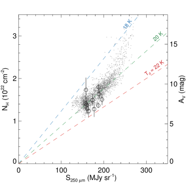
Figure 2: Hydrogen column density vs. 250 µm brightness towards the Cas A SNR. $N_{\rm H}$ is derived from either NIR [Fe II] line ratios (black empty circles; Section 3) or X-ray analysis (gray dots; Hwang & Laming, 2012). $S_{250~{}\micron}$ is obtained from Herschel SPIRE 250 µm image after subtracting synchrotron continuum. The dashed lines show the expected $S_{250~{}\micron}$ of the ISM of $N_{\rm H}$ with dust at $T_{\rm d}=18$, 20, and 22 K. The right $y$-axis shows the visual extinction ($A_{\rm V}$) corresponding to $N_{\rm H}$ for the general ISM, i.e., $A_{\rm V}/N_{\rm H}=1.87\times 10^{21}$ mag cm^-2 (Draine, 2003).

For an analysis of line flux ratios, we need to apply an extinction correction to the observed fluxes. The extinction to Cas A is large and varies significantly over the field, e.g., $A_{V}=5$–15 (Eriksen et al., 2009; Lee et al., 2015; Koo et al., 2018, and references therein). A column density map of the foreground gas/dust across the Cas A SNR had been obtained from X-ray spectral analysis (Hwang & Laming, 2012), but our target knots are mostly outside this column density map. For the knots with both [Fe II] 1.26 µm and 1.64 µm lines detected, we can derive extinction by using the flux ratio of these two lines because they share the same upper level (see, e.g., Koo & Lee, 2015; Lee et al., 2017). We, however, only obtained $H$-band spectra for the knots in Mask 1, and also some knots do not show any detectable [Fe II] lines. So, for the majority of the knots, we could not use this technique either. We instead used the Herschel SPIRE 250 $\mu$m data for the extinction correction. The extinction toward Cas A is mostly due to the ISM in the Perseus spiral arm, so that the dust emission at 250 $\mu$m is a good measure of the extinction to Cas A (e.g., De Looze et al., 2017; Zhou et al., 2018a). Koo et al. (2018) showed that there is a good correlation between the Herschel SPIRE 250 $\mu$m surface brightness ($S_{250~{}\mu{\rm m}}$) and the X-ray absorbing column density ($N_{\rm H,\,X-ray}$) towards dense circumstellar knots scattered over the remnant. Their plot is reproduced in Figure 2, where we see that the correlation is linear at $N_{\rm H,\,X-ray}\lower 2.15277pt\hbox{$\;\buildrel<\over{\sim}\;$}2\times 10^{22}$ cm^-2 and that it is consistent with the 250 $\mu$m emission being from 20 K dust with the general ISM dust opacity, i.e., $S_{250~{}\mu{\rm m}}/N_{\rm H,\,X-ray}\approx 1.1~{}{\rm MJy}/10^{20}~{}{\rm cm}^{-2}$. For higher column densities, $S_{250~{}\mu{\rm m}}$ are considerably smaller than those expected from $N_{\rm H,\,X-ray}$, which could be either because some column densities are due to molecular clouds and the temperatures of dust associated with molecular clouds are lower, or because some column densities are due to H gas without dust (Koo et al., 2018; Hartmann et al., 1997). In the figure, we overplotted our target knots where both [Fe II] 1.26 µm and 1.64 µm lines have been detected with high ($>6$) signal-to-noise ratio. There are 11 such knots and their [Fe II] 1.26 µm/[Fe II] 1.64 µm line ratios range 0.57–0.75 corresponding to hydrogen column densities of $N_{\rm H}=1.2$–$1.8\times 10^{22}$ cm^-2 adopting a theoretical line ratio of 1.36, which is the value suggested by Nussbaumer & Storey (1988a) and Deb & Hibbert (2010), and the dust opacity of the general ISM (Draine, 2003). We see that the column densities derived from the [Fe II] line ratios are generally consistent with the 250 $\mu$m brightness although there is a considerable uncertainty in the former, i.e., the Einstein $A$-coefficients of the two lines are uncertain and the [Fe II] 1.26 µm/[Fe II] 1.64 µm line ratios in literature range from 0.98 to 1.49 (see Giannini et al., 2015; Koo & Lee, 2015, and references therein). In this work, we have derived the absorbing column densities $N_{\rm H}$ for the 67 knots using Herschel SPIRE 250 µm image as described above, and applied an extinction correction to the observed line fluxes by using the extinction curve of the general ISM (Draine, 2003). The derived column densities for individual knots are listed in Table 3. Note that the uncertainty in the extinction correction will not significantly affect the results of our analysis using the $J$-band line ratios, e.g., an error of $5\times 10^{21}$ cm² in $N_{\rm H}$ would yield an error of $\sim 10$% in the extinction-corrected ratios of [S II] 1.03 µm and [Fe II] 1.257 µm line fluxes.

In addition to the 67 knots, we also detected “extended H emission features” in three slits (2-14, 2-15, 3-18) in the eastern outer region with a P.A. of $\sim 90\arcdeg$. They only show hydrogen lines, without any metallic emission lines. They will be discussed in Section 5.4, where we show that they are most likely arising from the interstellar/circumstellar medium rather than the SN ejecta.

4 Result

4.1 Line Ratios and Their Regional Characteristics

Figure 3 shows the locations of the observed knots and their line flux ratios of three bright emission lines (i.e., [S II] 1.03 µm, [P II] 1.189 µm, and He I 1.083 µm lines) to [Fe II] 1.257 µm line: hereafter $R$([S II]/[Fe II]), $R$([P II]/[Fe II]), and $R$(He I/[Fe II]). In the left panel, the line flux ratios are plotted as a function of the knot’s radial distance from the explosion center, while in the right panel, the locations of the knots are shown in the (R.A., Dec.) plane. In all frames, the color of the symbols represents the flux ratios, i.e., red (blue) means low (high) ratios. The square and circle symbols indicate the knots in the NE jet and Fe K plume areas, respectively. The red and green dashed lines in the right panel indicate the nominal location of the forward and revere shocks, respectively. We can see that the NE jet knots are located outside of the forward shock, while most of the knots in the Fe K plume area are located between the forward and reverse shocks except one at ${\rm P.A.}=142\arcdeg$ which apparently is located outside the forward shock.

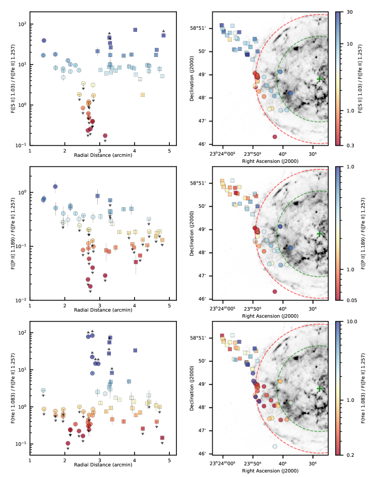
Figure 3: Identified NIR ejecta knots and their line ratios. The rows represent different line ratios: $R$([S II]/[Fe II]) at the top, $R$([P II]/[Fe II]) in the middle, and $R$(He I/[Fe II]) at the bottom. The left columns displays the line ratio against the knot’s radial distance from the explosion center, while the right column shows the locations of the knots in the (R.A., Dec.) plane. In all frames, the square and circle symbols indicate the NE jet area and Fe K plume area knots, respectively, and their colors represent the flux ratios as in the color bars. The red and green dashed lines in the right frame represent the nominal location of the forward and reverse shocks at 2017 epoch, $2\farcm 78$ and $1\farcm 85$, respectively (Gotthelf et al., 2001; DeLaney & Rudnick, 2003).

The ratio $R$([S II]/[Fe II]) of the ejecta knots varies over almost two orders of magnitude, i.e., 0.2 to 70 (see top row in Figure 3). A noticeable feature is a group of knots with low $R$([S II]/[Fe II]) at $r\sim 2\farcm 7$. Most of them have a strong [Fe II] 1.257 µm line without any detectable [S II] 1.03 µm lines, so they are marked with upper limits in the figure. They are knots located around the forward shock front just outside the Fe K plume. Their $R$([S II]/[Fe II]) upper limits are more than one or two orders of magnitude lower than the $R$([S II]/[Fe II]) of the knots around the reverse shock at $r=1\farcm 4$. There also appears to be a systematic variation in the $R$([S II]/[Fe II]) of the knots at $r\lower 2.15277pt\hbox{$\;\buildrel<\over{\sim}\;$}2.3$, i.e., the knots at larger radial distances have smaller ratios: The knots at $r=1\farcm 4$ have the ratios of a few 10s, while those at $r\sim 2\farcm 3$ have the ratios of $\sim 10$. On the other hand, the NE jet knots, except one, have $R$([S II]/[Fe II])$>4$, which is comparable with those of the knots around the reverse shock. There is no systematic variation in the $R$([S II]/[Fe II]) of the NE jet knots.

The ratio $R$([P II]/[Fe II]) shows a similar pattern to the $R$([S II]/[Fe II]), i.e., the knots at $r=2\farcm 7$ have a very low $R$([P II]/[Fe II]), and the knots at smaller radial distances have higher ratios (see middle row in Figure 3). Again, most of the knots around $r=2\farcm 7$ have no detectable [P II] 1.189 µm line. Most of the NE jet knots also have low $R$([P II]/[Fe II]), substantially lower than those of the knots around the reverse shock. Especially, most of the knots at $r\gtrsim 4\arcmin$ do not have any detectable [P II] 1.188 µm line. The $2\sigma$ upper limits of these knots are 0.05–0.3, which are a factor of 3–15 smaller than the ratios of the knots around the reverse shock.

The ratio $R$(He I/[Fe II]) between the knots differs by a factor of $10^{3}$ (see bottom row in Figure 3). For most knots located at $r<2\farcm 8$, the He I 1.083 µm line is not detected, and the upper limit of the $R$(He I/[Fe II]) is 0.1–1.0. However, knots of high ratio abruptly appear at $r\sim 3\farcm 0$ and the ratio reaches up to 100. Several knots in the NE jet area near $r\sim 3\farcm 0$ also show exceptionally high $R$(He I/[Fe II]). Seven knots were identified that exhibit only He I 1.083 µm line with/without very weak [C I] 0.985 µm line. These knots will be referred to as “He I knots” for the rest of the paper. These He I knots are detected mainly along the forward shock from the southern base of the NE jet to the Fe K plume area. It is worth mentioning that the radial velocities of the most of the He I knots are very large, so they are not circumstellar material (see § 5.2). In the NE jet, the knots near the tip of the jet have low ($\lower 2.15277pt\hbox{$\;\buildrel<\over{\sim}\;$}1.0$) $R$(He I/[Fe II]).

4.2 Classification of Knots and Their Physical Conditions

4.2.1 Knot Classification

In the previous section, we have found that the ejecta knots in different areas show distinct NIR spectroscopic properties. In this section, we classify the knots by using three line ratios; $R$([S II]/[Fe II]), $R$([P II]/[Fe II]), and $R$(He I/[Fe II]). We use [S II] 1.03 µm multiplet line instead of [S III] 0.953 µm line. The two lines have a good correlation and the latter is usually brighter than [S II] 1.03 µm multiplet, i.e., $F$([S III] 0.953)/$F$([S II] 1.03) = $1.5\pm 0.6$. But [S III] 0.953 µm line is very close to the blue limit of the spectroscope throughput, so the line becomes hardly detectable if it gets significantly blue-shifted (e.g., if its radial velocity is less than $-2000~{}{\rm km~{}s}^{-1}$). There are two knots emitting only weak [S III] 0.953 µm lines, but the expected [S II] 1.03 µm fluxes of those two knots from $F$([S III] 0.953)/$F$([S II] 1.03)=1.5 are smaller than their $3\sigma$ rms noise levels, indicating that the non-detection of the [S II] line is probably due to the low sensitivity of our observations. For these two knots, we use the expected [S II] 1.03 µm flux for their classification for convenience.

Figure 4: Classification of the NIR knots in $R$([S II]/[Fe II]) vs $R$([P II]/[Fe II]) plane. The square and circle symbols indicate the knots in the NE jet and Fe K plume areas, respectively. The arrows represent $2\sigma$ upper/lower limits. The black dashed line marks the boundary between the S-rich (blue) and Fe-rich (red) knots. The number of knots belonging to the two groups are given in parenthesis. The number (44) of the S-rich knots includes five knots that could not be not shown in the figure because only [S II] lines are detected. There are also seven He I knots where these metal lines are not detected (see § 4.2.1).

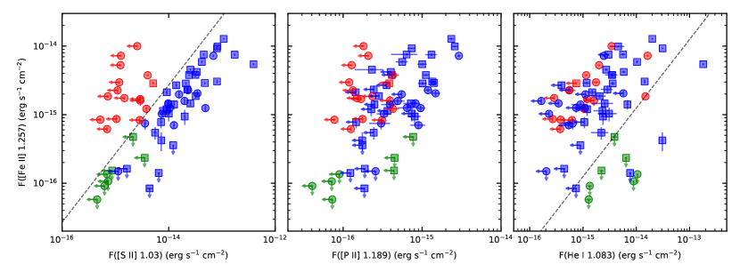
Figure 5: $F$([Fe II]) versus $F$([S II]), $F$([P II]), and $F$(He I). The knot symbols and their red and blue colors are the same as in Figure 4. The green symbols represent He I knots. The arrows represent $2\sigma$ upper/lower limits. The dashed line in the left frame marks the boundary between S-rich and Fe-rich knots. The dashed line in the right frame is the line at which $R$(He I/[Fe II])=8. The He I knots have $R$(He I/[Fe II]) higher than this.

Figure 4 is a diagram of $R$([P II]/[Fe II]) versus $R$([S II]/[Fe II]). The NE jet area knots and Fe K plume area knots are marked by squares and circles, respectively. We first examine $R$([S II]/[Fe II]) of the knots. The $R$([S II]/[Fe II]) of the knots ranges from 0.2 to 70. The Fe K plume area knots are scattered over the entire range, while the NE jet knots have relatively high ratios, i.e., $R$([S II]/[Fe II])$\lower 2.15277pt\hbox{$\;\buildrel>\over{\sim}\;$}4$. Note that most of the Fe K plume area knots with $R$([S II]/[Fe II])$\lower 2.15277pt\hbox{$\;\buildrel<\over{\sim}\;$}4$ do not have detectable [S II] emission. Such separation of the knots in $R$([S II]/[Fe II]) is similar to the properties of the knots in the main ejecta shell. For the knots in the main ejecta shell, Lee et al. (2017) performed principal component analysis of their NIR spectral properties and showed that they could be classified into two groups; (1) S-rich knots showing strong [S II] and [P II] lines and (2) Fe-rich knots showing strong [Fe II] lines. They found that the two groups were well divided by the ratio $F$([S II] 1.03)/$F$([Fe II] 1.644) of $\sim 5$. Following Lee et al. (2017), we adopt the threshold of $R$([S II]/[Fe II])$\sim 3.7$ assuming the intrinsic ratio of 1.36 for $F$([Fe II] 1.257 )/$F$([Fe II] 1.644) (Nussbaumer & Storey, 1988b; Deb & Hibbert, 2010). We therefore divide the knots into two groups; “S-rich knots” with $R$([S II]/[Fe II]) $\geq 3.7$ and “Fe-rich knots” with $R$([S II]/[Fe II]) $<3.7$. In Figure 4, S-rich and Fe-rich knots are represented by blue and red symbols, respectively. Note that all Fe-rich knots except one are the knots in the Fe K plume area and that almost of all of them have no detectable [S II] and [P II] emission. The Fe-rich knots are mostly located around the outer boundary of the Fe K plume (see Figure 3), and, as we will discuss in § 5.2, it has an interesting implication on the SN explosion dynamics. Another thing to note is that all NE jet knots except one are S-rich knots and that they have $R$([P II]/[Fe II]) ratios generally lower than those of the S-rich knots in the Fe K plume area (see also Figure 3). We will explore the spectral properties of the NE jet knots in detail in § 5.1.

Figure 4 does not include all 67 ejecta knots because some knots do not exhibit [Fe II] 1.257 µm (and [P II] 1.189 µm) lines. This may appear strange because our target knots have been selected from the deep [Fe II] image. But the observation was done with a $10^{\prime\prime}$ slit in ABBA mode, so there could be non-[Fe II]-emission knots accidentally located within the slit. There are 12 knots with no detectable [Fe II] 1.257 µm lines. Among these, four knots show only [S II] 1.257 µm and/or [S III] 0.953 µm lines, one knot shows only [S II]  1.257 µm and He I 1.083 µm lines, and seven knots show only He I 1.083 µm lines. The former five knots belong to S-rich knots because [Fe II] 1.257 µm line has not been detected. (Their $2\sigma$ lower limits of $R$([S II]/[Fe II]) are $\geq 3.7$.) But $R$([P II]/[Fe II]) is not available for them because both [Fe II] 1.257 µm and [P II] 1.189 µm lines are not detected. Then there are seven He I knots that show only He I 1.083 µm line with no [S II] 1.03 µm, [Fe II] 1.257 µm, and [P II] 1.189 µm lines. Their He I 1.083 µm fluxes are comparable to those of the metal-rich ejecta knots, but their [S II] 1.03 µm, [Fe II] 1.257 µm, and [P II] 1.189 µm fluxes are considerably lower than those of the other ejecta knots (Figure 5). We note that these He I knots are mostly an accidental detection and that the category of the He I knots is not very rigorously defined. Indeed some spectra of S/Fe-rich knots with high $R$(He I/[Fe II])  if degraded, could become indistinguishable from the He I knots. However, the number of such knots is less than a few thus should not affect our discussion on He I knots. From Figure 5, we can also see that S-rich and Fe-rich knots have a comparable range of [Fe II] 1.257 µm line strengths. This is not unexpected, given that the knots that we observed are the bright ones in the deep [Fe II] image. The two groups of the knots, however, are clearly distinguished in their [S II] line fluxes. In [P II] emission, the Fe-rich knots generally have lower 1.189 µm fluxes than the S-rich knots, but not necessarily. A good fraction of the S-rich knots have [P II] 1.189 µm fluxes as low as the Fe-rich knots. As we will see in § 5.1, they are the knots near the tip of the NE jet.

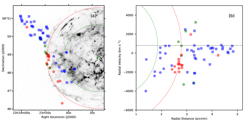
Figure 6: Spectral properties of the 67 ejecta knots shown in (a) (RA, Dec) and (b) (radial distance, radial velocity) planes. The spectral properties are color-coded: S-rich knots in blue and Fe-rich knots in red. The He I knots are shown in green. The background in (a) is a Chandra X-ray 4.2–6.4 keV image produced from the data taken in 2013–2017. The dashed lines and the green cross symbol are the same as in Figure 3. The gray dashed line in the right frame indicates the systematic velocity centroid of the remnant, $v_{r}=+800~{}{\rm km~{}s}^{-1}$ (Reed et al., 1995; DeLaney et al., 2010; Isensee et al., 2010; Milisavljevic & Fesen, 2013).

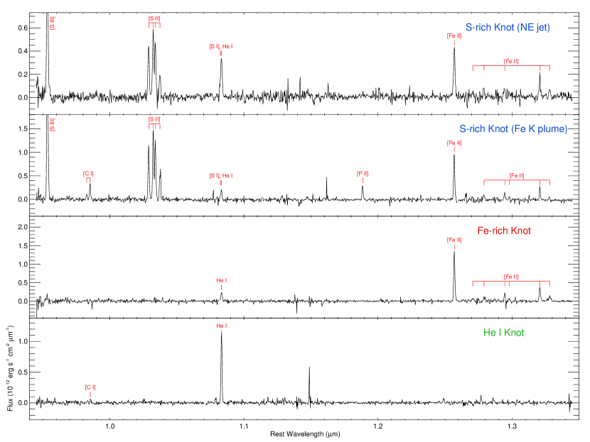
Figure 7: Sample 1-D spectra of three ejecta knot groups: S-rich knots (2-06-1, 1-18-1), Fe-rich knots (1-16-1), and He I knots (2-15-2). For the S-rich knots, separate sample spectra are shown for the NE jet and Fe K plume areas because the intensities of the [P II] 1.189 µm line differ significantly between the two regions. The positions of the knots are marked in Figure 1. The spiky features in the spectra are the residuals of bright OH airglow emission lines.

In summary, we have classified the 67 knots into three groups: S-rich (44), Fe-rich (16), and He I knots (7). Figure 6 shows which group each individual observed knots belong to. We see that the majority (31/35) of the NE jet knots are S-rich knots. Only one knot is classified as Fe-rich, which has R([S II]/[Fe II])(=1.8) close to the threshold dividing S-rich and Fe-rich knots. For comparison, the majority (26/32) of the Fe K plume area knots are S-rich or Fe-rich with clear spatial separation between them: the S-rich knots are near the main ejecta ring within the SNR, while the Fe-rich knots are aligned in the north-south direction along the boundary of the SNR. Figure 6 also shows that those Fe-rich knots appear to be clustered in the position-velocity diagram, implying that they were ejected in a narrow cone. We will explore the kinematic properties of the Fe-rich knots in § 5.2. The He I knots are detected along the forward shock front, from the southern base of the NE jet to the Fe K plume area. Most of the He I knots have large radial velocities, so they are different from the circumstellar knots bright in He I 1.083 µm line (see Lee et al., 2017). We will explore their origin in § 5.2. Table 5 summarizes the properties of the three groups, and Figure 7 shows the representative sample spectra of individual groups.

4.2.2 Spectral and Physical Properties of Three Knot Groups

In this section, we examine the basic spectral properties of three knot groups and compare the densities of their line-emitting regions, looking for differences other than the bright line ratios.

Figure 8 compares the distributions of the radial velocities and line widths of three knot groups. The radial velocities of the S-rich knots strongly peaks near 0 ${\rm km~{}s}^{-1}$, which is mostly due to the knots in the NE jet. The radial velocities of the knots in the NE jet are mostly confined to a narrow range of $v_{\rm r}=0$ to $+800~{}{\rm km~{}s}^{-1}$, but there are also knots with high positive and high negative velocities, e.g., the radial velocities of the knots in the southernmost stream are $v_{\rm r}=-2100$ ${\rm km~{}s}^{-1}$ to $-520$ ${\rm km~{}s}^{-1}$. This is consistent with the previous result from optical studies that the bright knots in the jet streams lie close to the plane of the sky although the knots in the NE jet region including those in the jet base area in general encompasses a broad range of radial velocities (Fesen & Gunderson, 1996; Fesen, 2001; Milisavljevic & Fesen, 2013). For comparison, the S-rich and Fe-rich knots in the Fe K plume area are mostly blueshifted. As already mentioned in § 4.2.1, the Fe-rich knots are mostly located in the Fe K plume area and their radial velocities are confined to a narrow range ($-2000$ to $-$200 ${\rm km~{}s}^{-1}$). On the other hand, the radial velocities of the He I knots are spread over a broad velocity range, from $-3500$ ${\rm km~{}s}^{-1}$  to +3500 ${\rm km~{}s}^{-1}$. In line width, the S-rich knots have a broad distribution centered at around +290 ${\rm km~{}s}^{-1}$, while the Fe-rich and He-rich knots have a relatively narrow distribution centered at approximately +250 ${\rm km~{}s}^{-1}$. The velocity widths may be considered as a characteristic shock speed for the knots. But as we will see in § 4.3, the ejecta knots appear to have complex structures with subknots, so the shock speed could be substantially lower than this. Figure 8 also compares the distribution of [Fe II] 1.257 µm line fluxes among the three knot groups. As we already mentioned in § 4.2.1, the S-rich and Fe-rich knots have a similar distribution of [Fe II] 1.257 µm line fluxes, while the He I knots have [Fe II] 1.257 µm line undetected with an upper limit mostly a few times $10^{-16}$ erg s^-1 cm² (see Figure 3). Note that [Fe II] 1.257 µm line flux in the table is the flux within the slit. The fluxes of the knots in the deep [Fe II] image may be found in Koo et al. (2018).

Figure 8: Distribution of the spectral parameters of the knots in three knot groups. The columns represent different parameters: radial velocity, line width, and [Fe II] 1.257 µm flux. The rows represent different knot groups. In each frame, the light-colored histogram represents the knots in the NE jet area and the dark-colored histogram represents the knots in the Fe K plume area.

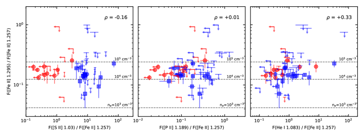
Figure 9: $F$([Fe II] 1.295)/$F$([Fe II] 1.257) versus $R$([S II]/[Fe II]), $R$([P II]/[Fe II]), and $R$(He I/[Fe II]). The knot symbols and colors are the same as in Figure 4. The horizontal lines mark the $F$([Fe II] 1.295)/$F$([Fe II] 1.257) ratios of ionized gas of $n_{e}=10^{3}$, $10^{4}$, and $10^{5}$ cm^-3 at $10^{4}$ K in collisional equilibrium. The parameter $\rho$ in each frame is the correlation coefficient between two ratios.

One of the physical parameters of the knots that can be easily obtained is electron density. In the J and H bands, there are several [Fe II] lines originating from levels with similar excitation energies, whose ratios depend mainly on electron densities and can be used as a density tracer (e.g., see Koo et al., 2016; Lee et al., 2017). In Figure 9, we plot $F$([Fe II] 1.295)/$F$([Fe II] 1.257) of the knots, which is sensitive to electron density between $10^{3}$ cm^-3 and $10^{5}$ cm^-3. The $x$-axes of the frames in the figure are [S II] 1.03 µm, [P II] 1.189 µm, and He I 1.083 µm fluxes normalized by [Fe II] 1.257 µm flux. For about two thirds of the knots, [Fe II] 1.295 µm line has not been detected, so their upper limits are plotted. For the knots with [Fe II] 1.295 µm line detected, the electron densities inferred from their [Fe II] line ratios are mostly in the range of (1–4)$\times 10^{4}$ cm^-3, with the mean of 1.8$\times 10^{4}$ cm^-3. The S-rich knots have a slightly lower density than the Fe-rich knots, i.e, 1.5$\times 10^{4}$ cm^-3 vs 2.5$\times 10^{4}$ cm^-3. Note that this is the density of shock-compressed, line-emitting region of the knots. The initial density of a knot before being shocked should be much lower (e.g., $\sim 10^{2}$ cm^-3; see Figure S3 of Koo et al. 2013). There is no clear association between the line ratios of the bright lines and $F$([Fe II] 1.295)/$F$([Fe II] 1.257), except for a moderate positive correlation ($\rho=+0.33$) observed for $R$(He I/[Fe II]), which could be possibly because the He I 1.083 µm line emissivity increases with density due to the contribution from the collisional excitation from the lower level ($2{{}^{3}}$S) (e.g., see Koo et al., 2023). For a given $F$([Fe II] 1.295)/$F$([Fe II] 1.257) ratio, the $R$([S II]/[Fe II]) of S-rich and Fe-rich knots differs by more than an order of magnitude. This suggests that the density of the shocked gas is not the primary factor causing the division between the two groups of ejecta knots.

4.3 Optical Counterparts

Numerous dense ejecta knots have been identified around the Cas A SNR in previous optical studies, and it will be interesting to check if our NIR ejecta knots have optical counter parts. We use the optical ejecta knot catalog of Hammell & Fesen (2008), who identified 1825 compact optical knots that lie beyond a radial distance of $\sim 2\arcmin$ from the explosion center in Hubble ACS/WFC images taken with three different broadband filters (i.e., F652W, F775W, F850LP) in 2004. They were able to classify the optical knots into three groups based on their flux ratios in the three filters: (1) [N II] knots dominated by [N II] $\lambda\lambda$6548, 6583 emissions, (2) [O II] knots dominated by [O II] $\lambda\lambda$7319, 7330 emissions, and (3) Fast-Moving Knot (FMK)-like knots displaying filter flux ratios suggestive of [S II], [O II], and [Ar III] $\lambda$7135 emission line strengths similar to the FMKs found in the remnant’s main ejecta shell (see also Fesen et al. 2006). Of the 1825 knots identified by them, 444 were [N II] knots, 192 were [O II] knots, and 1189 were FMK-like knots. Their spatial distribution are distinct; [N II] knots are arranged in a broad shell around the remnant, [O II] knots are clustered around the base of jets, and FMK-like knots are mainly confined to NE and SW jet areas (see also Fesen & Milisavljevic 2016). We have compared the spatial positions of our 67 NIR ejecta knots with those of the optical outer knots shifted to 2017 epoch assuming free expansion. Considering the seeing and slit width of our observations, we have searched their optical counterparts within 0$\farcs$5 radius. Note that 12 out of the 67 ejecta knots are located inside $r=2\farcm 4$ where Hammell & Fesen (2008) did not search optical knots, so we can check the counterparts only for 55 NIR knots.

Figure 10: Optical counterparts of the sample of NIR knots detected in slits 1-9, 1-16, 2-12, and 3-23. For each slit area, four images are shown: the deep [Fe II] image and three HST images obtained with F098M, F625W, and F850LP filters. North is up, and east is to the left. In each frame, the gray rectangle represents the location of the 10″-long MOS slit, and the circles mark the knot locations, the colors of which represent the knot groups: S-rich knots in blue, Fe-rich knots in red, and He I knots in green. Note that the positions of the slits and the circles are shifted to the epochs of the background images, which are given at the top of individual columns.

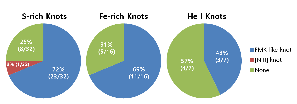
Figure 11: Pie charts showing the optical counterparts of 55 NIR ejecta knots. The red and blue slices represent the percentages of the NIR knots with optical [N II] and FMK-like knots as counterparts, respectively, while the green slice represents the percentage of the NIR knots without optical counterparts. Note that the statistics of S-rich knots includes only 32 knots out of 44. The rest twelve S-rich knots are located in the inner region of the Cas A SNR where the characteristics of the optical knots were not investigated by Hammell & Fesen (2008).

We found that 38 out of the 55 NIR knots have optical counterparts. All of them have FMK-like knots as a counterpart except one that appears to have an [N II] knot as a counterpart. No NIR knots have [O II] knots as a counterpart. It is not unusual that the NIR knots that are identified from the ground-based, deep [Fe II] image are resolved into multiple knots in high resolution HST images, implying that the knots can have a complicated structure consisting of subknots. Figure 10 shows optical counterparts of the sample of the observed NIR knots. Some NIR knots appear as a single, very compact optical knot, but they often have a more complex structure that is resolved into smaller subcomponents. In some cases, an NIR knot is found to be a part of a larger, more extended structure in optical. We further note that optical knots tend to cluster together with other knots of the same type. However, there are rare cases where different types of optical knots are found in close proximity to each other, especially in the main shell region. While these can complicate the identification of optical counterparts, we do not think the overall trend will be affected. Figure 11 shows the pie charts for the optical counter parts of the three groups of the NIR knots. About three quarters of S-rich and Fe-rich knots have optical counterparts, while about half of He I knots has optical counterparts. It is worth noticing that one quarter of S-rich knots has no optical counterpart, although, since the F850LP filter is sensitive to [S II] 1.03 µm and [S III] 0.907, 0.953 µm lines, the S-rich knots emitting strong [S II] and [S III] lines should be detected at least in the deep F850LP image. These S-rich knots not detected in the deep optical image may have appeared after 2004 when the HST images were taken: It has been found that the knots in the NE jet and Fe K plume areas reveal substantial emission variations (“flickering”) in an interval as short as nine months (Fesen et al. 2011; see also Figure 10). Indeed, we were able to confirm that several knots (e.g., Knots 2, 7, 15) were not present in the 2004 HST image but appeared in a subsequent 2010 HST image.

We also found that 70% of the Fe-rich knots have FMK-like knots as their optical counterparts. This is inconsistent with our results that most Fe-rich knots do not have [S II] 1.03 µm and [S III] 0.953 µm lines. One possibility is that the flux detected in the F850LP image is not due to [S II] or [S III] lines but [Fe II] lines. There are several bright [Fe II] lines, e.g., 8619 Å, 8894 Å, 9229 Å (Dennefeld, 1986; Hurford & Fesen, 1996; Koo et al., 2016), in the wavelength band (8000–10,000 Å) of the F850LP filter, while no or little bright [Fe II] lines in the wavebands of the F652W and F775W filters. For example, the expected [Fe II] $\lambda$8619/[Fe II]$1.257\mu$m ratio ranges from 0.08–0.49 for electron densities $10^{3}$–$10^{5}$ cm^-3 (Koo et al., 2016). Hence, [Fe II] lines can make a substantial contribution to the F850LP filter flux, and, together with the high interstellar extinction toward Cas A, the Fe-rich knots in out sample could have been classified as FMK-like knots in optical band. Note that the majority of the optical knots in the catalog of Hammell & Fesen (2008) are very faint with the F850LP flux less than $5\times 10^{-17}$ erg cm^-2 s^-1, which is more than two orders of magnitude smaller than the [Fe II] 1.257 µm fluxes of Fe-rich knots (Figure 5). Another possibility is that the knots have [S II] and/or [S III] lines but the lines are ‘weak’, i.e., $R$([S II]/[Fe II])$<3.7$, so they have been classified as Fe rich knots in this work, but they were detected in the deep F850LP image and classified as FMK-like knots. Indeed, at least three of the Fe rich knots with FMK-like knot counterparts do have [S II] lines (see Table 6 in § 5.2). Yet another possibility is a chance coincidence. The area where the Fe-rich knots have been detected are crowded with the FMK-like knots (e.g., see Figure 1 of Hammell & Fesen 2008), so that we cannot rule out the possibility that a FMK-like knot accidentally falls within the circle of $0\farcs 5$ radius. But, since the distances between the matched knots are usually an order of magnitude smaller the median distance between the optical knots around Fe-rich knots (i.e., a few arcseconds), most of the matches are probably genuine.

Lastly, it is interesting that about half of the He I knots has FMK-like knots as their optical counter parts. This may indicate that He I knots are just S-rich knots with [S II], [S III], and [Fe II] lines below our detection limit. But, since most of the He I knots are also located in the area crowded with FMK-like knots, a chance coincidence is possible. We will explore the nature of He I knots in § 5.3.

5 Discussion

5.1 S-rich Ejecta Knots in the NE Jet

A most striking morphological feature in Cas A known from early optical studies is the NE jet structure (van den Bergh & Dodd, 1970; Fesen & Gunderson, 1996). It is composed of the streams of bright knots confined into a narrow cone well outside the northern SN shell that appears to have punched through the main ejecta shell. The jet structure extends to $\sim 3^{\prime}$ out beyond the main shell implying the ejection velocities upto 16,000 ${\rm km~{}s}^{-1}$, which is three times faster than the bulk of the O- and S-rich ejecta in the main ejecta shell (Kamper & van den Bergh, 1976; Fesen & Gunderson, 1996; Fesen, 2001; Fesen & Milisavljevic, 2016). Later the SW “counterjet” composed of numerous optical knots with comparable maximum expansion velocities was detected on the opposite side (Fesen, 2001; Milisavljevic & Fesen, 2013). The origin of the bipolar NE jet–SW counterjet structure is not fully understood although it must have been generated very near the explosion center during the first seconds of the explosion (see below). A critical information for the origin of the jet comes from its chemical composition. Previous optical studies showed that the NE jet knots exhibit strong S, Ca, and Ar emission lines with comparatively weak oxygen lines (van den Bergh, 1971; Fesen & Gunderson, 1996; Fesen, 2001; Hammell & Fesen, 2008; Milisavljevic & Fesen, 2013; Fesen & Milisavljevic, 2016). The knots lying farther out and possessing the highest expansion velocities show no detectable emission lines other than those of [S II] (Fesen & Milisavljevic, 2016). The knots near the jet base, on the other hand, show O and N emission too (Fesen & Gunderson, 1996). The jet structure has been observed in X-ray and IR too. In X-ray, the jet material shows strong Si, S, Ar, and Ca lines but not particularly strong Fe K line (Hughes et al., 2000; Hwang et al., 2004; Vink, 2004). Fe K emission has been found to be strong in other areas of Cas A, particulary in the eastern area (Hwang & Laming, 2003, 2012; Picquenot et al., 2021, see § 5.2). These X-ray studies showed that the elemental composition of the jet, enriched in the intermediate-mass elements with a limited amount of Fe, is similar to that of oxygen or incomplete Si burning (see also Ikeda et al. 2022). In IR, the ring-like jet base lifted from the main ejecta shell is pronounced in Ar emission (DeLaney et al., 2010). These findings suggest that the jet originated in the deep interior of the progenitor star where Si, S, Ar, and Ca are nucleosynthesized and penetrated through the outer stellar envelope.

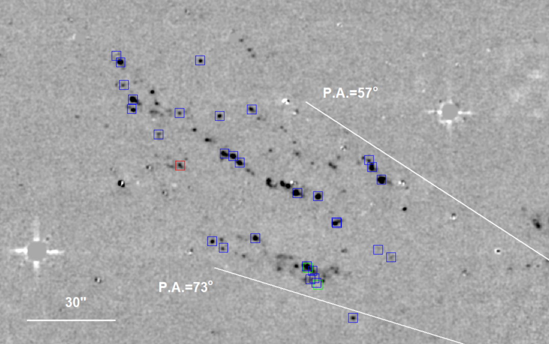
Figure 12: Detail of the NE jet area. The background is the deep [Fe II] image. North is up, and east is to the left. The knots where NIR spectra have been obtained in this work are marked by squares, the colors of which represent the knot groups: S-rich knots in blue, Fe-rich knots in red, and He I knots in green.

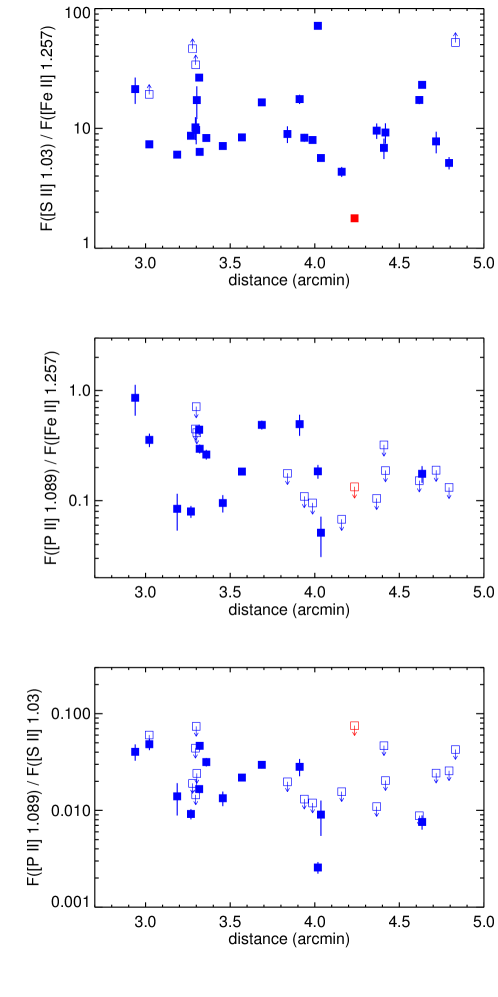
Figure 13: Line ratios of the NE jet knots as the function of distance from the explosion center. S-rich and Fe-rich knots are denoted by blue and red squares, respectively, while empty symbols indicate upper limits.

Figure 12 gives a detailed view of the NE jet structure in [Fe II] 1.644 µm emission. In the image, the NE jet appears as streams of bright knots confined to a fanlike structure with an opening angle of 10$\arcdeg$ viewed at the explosion center. The central stream at P.A.$\simeq 64\arcdeg$ is most prominent, extending to $4\farcm 7$($=4.6$ pc) from the explosion center. In the northern area above the central stream, there are many bright knots scattered over the area that appear to be aligned along several stream lines, while, in the southern area below the central stream, there is a prominent but fuzzy stream of ejecta material possessing a finite width at P.A.$\simeq 70\arcdeg$, and not many bright knots are in between. This jet morphology is very similar to what we have already seen in [S II] $\lambda\lambda$ 6716, 6731 emission (Fesen & Gunderson, 1996).

In Figure12, we marked the ejecta knots observed in this work using different colors for S-rich, Fe-rich, and He I knots. We see that the NE jet knots are mostly S-rich (see also Figure 6). We have not detected an Fe-rich knot exhibiting only [Fe II] lines. There is one knot classified as a Fe-rich knot located between the central and the southern streams, but it exhibits [S II] lines of moderate strength ($R$([S II]/[Fe II])=1.8). These results are consistent with the previous results from optical and X-ray studies that the jet material shows strong S lines but not particularly strong Fe lines. In optical bands, the NE jet knots show strong O, S, Ar lines like the other S-rich knots and are not clearly distinguished from the S-rich knots (FMKs) in the main ejecta shell, although, for example, a few outermost knots show stronger than usual [Ca II] $\lambda\lambda$7291, 7324 lines that could be due to abundance difference (Fesen & Gunderson, 1996). In NIR, however, the NE jet knots are distinguished from the S-rich knots in the main ejecta shell in [P II] emission: The majority of the dense knots in the NE jet show weak or no [P II] lines whereas the S-rich knots in the main ejecta shell show strong [P II] lines. This is shown in Figure 13, where the line ratios of the NE jet knots are plotted as a function of distances from the explosion center (see also Figure 3). The figure shows that $R$([S II]/[Fe II]) remains roughly constant along the jet, whereas $R$([P II]/[Fe II]) and $R$([P II]/[S II]) appear to decrease systematically along the jet. Note that [P II] line has not been detected in the majority of the knots near the tip of the jet. For comparison, the three ratios for the S-rich knots in the main ejecta shell are ($R$([S II]/[Fe II]), $R$([P II]/[Fe II]), $R$([P II]/[S II]))=($14.2\pm 13.5$, $1.46\pm 1.31$, $0.117\pm 0.083$) (see Figure 2 of Koo et al., 2013).

The simplest interpretation of the low [P II]/[Fe II] and [P II]/[S II] ratios of the NE jet knots is that the amount of phosphorus present there is lower compared to the knots in the main shell. Although the knots in the NE jet and the main shell have different shock environments, the decrease in these ratios from the main shell to the tip of the NE jet, while the [S II]/[Fe II] ratio remains constant, suggests that the phosphorus abundance is probably the primary factor affecting the line ratios. Therefore, we consider the weakness of the [P II] line in the NE jet knots as direct evidence that the NE jet originated from a layer with a high sulfur and low phosphorus content. And, since ¹⁵P is mainly produced in carbon and neon burning layers (Arnett, 1996; Woosley et al., 2002), it implies that the NE jet was ejected from a region below the explosive Ne burning layer, i.e., O burning or incomplete Si burning layers. This is consistent with the result of previous X-ray studies, which showed that the elemental composition of diffuse ejecta material in the NE jet is similar to that of oxygen and incomplete burning (Vink, 2004; Ikeda et al., 2022).

We now discuss the implication of our results on the physical origin of the NE jet. The origin of the NE jet and its role in the SN explosion have been subject to study since its discovery in 1960s. Minkowski (1968) suggested that the jet structure (or the ‘flare’ in his paper) could be a surviving part of a spherically symmetric shell due to non-spherically distrbution of ambient interstellar medium (see also Fesen & Gunderson, 1996). But it is now rather well established that the NE jet originated from a Si-S-Ar rich layer deep inside the progenitor and penetrated through the outer N and He-rich envelope (Fesen, 2001; Fesen et al., 2006; Laming et al., 2006; Milisavljevic & Fesen, 2013). The chemical composition of the jet material and the spatial correlation between the jet and the disrupted main ejecta shell are strong evidence for that. On its launching mechanism, there have been several theoretical propositions in relation to the core-collapse SN explosion models. In the classical ‘jet-induced’ explosion model, where magnetic field anchored to the collapsing core is amplified during the collapse and drives the SN explosion, a magnetocentrifugal jet can be ejected along the rotation axis (Khokhlov et al., 1999; Wheeler et al., 2002; Akiyama et al., 2003). Recent observational studies, however, suggest that the properties of the NE jet are not consistent with the jet-induced explosion model; there is no ‘pure’ Fe ejecta in the jet (Ikeda et al., 2022), the opening angle is large and the kinetic energy is insufficient, and the kick direction of the neutron star kick is not along but perpendicular to the jet axis (Fesen 2001; Hwang et al. 2004; Laming et al. 2006; Milisavljevic & Fesen 2013; Fesen & Milisavljevic 2016; cf. Soker 2022). Our results are also in line with previous results and do not support the jet-scenario. We have not found dense Fe-rich knots around the tip of the NE jet either in this study. The opening angle of the jet in Figure 12 is small ($\lower 2.15277pt\hbox{$\;\buildrel<\over{\sim}\;$}15\arcdeg$), but their total kinetic energy will be less than the previous estimate of $1\times 10^{50}$ erg of the optical knots in the NE jet (Fesen & Milisavljevic, 2016). Hence, our results also do not support the jet-induced explosion model.

In the neutrino-driven explosion model, which is the modern paradigm of the core-collapse SN explosion, a narrow high-velocity ejecta can be generated either during the explosion or after the explosion by the newly-formed neutron star. During the explosion, high-speed jet-like fingers can be produced from the core by neutrino convection bubbles (e.g., Burrows et al., 1995; Janka & Mueller, 1996). In particular, the interface between Si and O composition is unstable seeded by the flow-structures resulting from neutrino-driven convection, leading to a fragmentation of this shell into metal-rich clumps (Kifonidis et al., 2003). Orlando et al. (2016a) showed that the Si-rich, jet-like features such as the NE jet in Cas A could be reproduced by introducing overdense knots moving faster than the surrounding ejecta just outside the Fe core. But a recent three-dimensional simulation for modeling the Cas A SNR as a remnant of a neutrino-driven SN, starting from the core-collapse to the fully developed remnant, could not reproduce a structure similar to the NE jet (Orlando et al., 2021). Another possibility is that hydrodynamic jet from a newly-formed neutron star. In a standard neutrino-driven explosion, a fraction of ejecta falls back to the newly-formed neutron star to form a disk where a MHD jet can be launched (Burrows et al., 2005, 2007; Burrows & Vartanyan, 2021; Janka et al., 2022). But, as far as we are aware, there is little theoretical prediction that can be compared with observation for such an MHD jet. So for the neutrino-driven explosion model, it is still an open question if the NE jet can be explained by this model.

5.2 Fe Ejecta Knots in the Fe K plume area

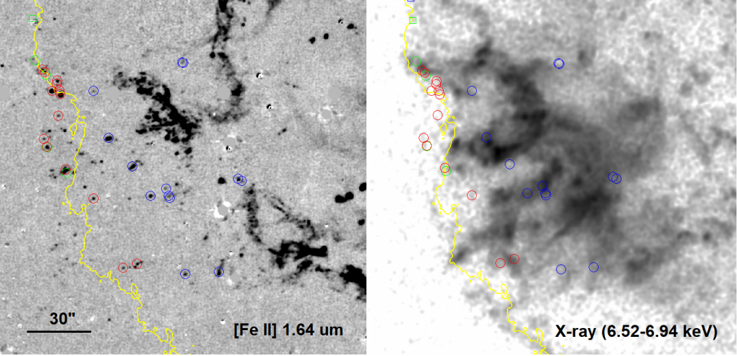
Figure 14: Detail of the Fe K plume area in the deep [Fe II] and Chandra X-ray Fe K emission images. North is up, and east is to the left. The knots where NIR spectra have been obtained in this work are marked by circles (P.A.$\geq 78^{\circ}$) or squares (P.A.$<78^{\circ}$), the colors of which represent the knot groups: S-rich knots in blue, Fe-rich knots in red, and He I knots in green. Note that the positions of the knot markers are shifted to the epochs of the background images, i.e., 2013 Sept. for the deep [Fe II] image and 2004 Apr. for the Chandra image. The yellow contour marks an approximate boundary of the SNR in radio in 2003 (DeLaney, 2004), and it is left as a reference point.

We discovered Fe-rich knots in the Fe K plume area (see Figure 14). This is the area where the Fe-rich plume with bright Fe K emission has been detected in X-ray (Willingale et al., 2002; Hwang & Laming, 2003; Hwang et al., 2004; Hwang & Laming, 2012; Tsuchioka et al., 2022). The ejecta material in this Fe K plume has no S or Ar, and its Fe/Si abundance ratio is up to an order of magnitude higher than that expected in incomplete Si-burning layer, indicating that they originated from complete Si-burning process with $\alpha$-rich freezeout, where the burning products are almost exclusively ⁵⁶Fe because free $\alpha$ particles are unable to reassemble to heavier elements on a hydrodynamic time scale (Arnett, 1996; Woosley et al., 2002). Recently, Sato et al. (2021) detected Ti and Cr in this area, the ratio of which to Fe is consistent with explosive complete Si burning with $\alpha$-rich freezeout. Therefore, the material in the Fe K plume has likely been produced in the innermost, high-entropy region during the SN explosion where the temperature is high and density is low (e.g., Arnett, 1996; Thielemann et al., 1996). In two-dimensional projected maps, however, the Fe K plume is located much further outside the main shell which is composed of ejecta synthesized from incomplete Si burning, e.g., Si, S, Ar, which could be interpreted as a overturning of ejecta layers (Hughes et al., 2000). But a three-dimensional reconstruction of the ejecta distribution using infrared and Chandra X-ray Doppler velocity measurements showed that, in the main shell, the Fe K plume occupies a “hole” surrounded by a ring structure composed of Si and Ar (DeLaney et al. 2010; see also Milisavljevic & Fesen 2013). As an explanation of the observed morphology, DeLaney et al. (2010) proposed a model where an ejecta “piston” faster than average ejecta has pushed through the Si layers rather than interpreting it as an overturning of the layers. In this model, the Si-Ar ring structure in the main shell represents the circumference of the piston intersecting with the reverse shock. Recently Tsuchioka et al. (2022) showed that the velocity of the ejecta in the outermost Fe K plume is $>4500$ ${\rm km~{}s}^{-1}$, much higher than that of Si/O-rich ejecta, suggesting that the ejecta piston has been formed at the early stages of the remnant evolution or during the SN explosion, which is consistent with the results of numerical simulations. On the other hand, recent 3-D numerical simulations demonstrated that Ni clumps, created during the initial stages of the SN explosion in the innermost region by the convective overturning in the neutrino-heating layer and the hydrodynamic instabilities, later decay to ⁵⁶Fe and can push out the less dense ejecta to produce structures such as Fe K plume (Orlando et al., 2016b, 2021). But Hwang & Laming (2003) pointed that the morphology and the ‘ionization age’ ($=n_{e}t$ where $n_{e}$ is electron density and $t$ is the time since the plasma was shock-heated) of the Fe ejecta in the Fe K plume are inconsistent with a Ni bubble origin.

Our detection of Fe-rich knots in the Fe K plume area has quite significant implication. Figure 14 shows the distribution of IR ejecta knots in the Fe K plume area. We see a group of Fe-rich knots aligned in the north-south direction along the forward shock front. They are spatially confined in the area immediately outside the boundary of the diffuse X-ray Fe ejecta. Their radial velocities are in a narrow range, from $-2000$ ${\rm km~{}s}^{-1}$ to $-$200 ${\rm km~{}s}^{-1}$ (see Figure 8 and Table 6), so, in a position-velocity diagram, they appear to be clustered (see Figure 6b). The ejection angle of this “Fe-rich ejecta knot cluster” is $14\arcdeg\pm 5\arcdeg$ from the plane of the sky toward us. (In Figure 6b, we see two Fe-rich knots located far off the cluster. One of them is Knot 23 in the NE jet area and the other is Knot 67 near the southern edge of the field. The latter has a radial velocity +1960 ${\rm km~{}s}^{-1}$, which is very different from those of the Fe-rich ejecta knot cluster. They are not considered to belong to the cluster.) The radial velocities of the X-ray emitting diffuse ejecta in this area measured with Chandra High Energy Transmission Grating are from $-2600$ to $-500$ ${\rm km~{}s}^{-1}$, comparable with those of the Fe-rich knots (Lazendic et al., 2006; Rutherford et al., 2013). On the other hand, the proper motion of Fe-rich knots has velocity of 6600–7600 ${\rm km~{}s}^{-1}$ (Table 6), which is considerably higher than those of the diffuse ejecta at the tip of the Fe K plume (i.e., 4500–6700 ${\rm km~{}s}^{-1}$, Tsuchioka et al. 2022). Hence, the Fe-rich knots move a little faster than the diffuse X-ray emitting Fe-rich ejecta. The spatial and kinematic relations strongly support the physical association between the dense Fe-rich knots and the X-ray diffuse Fe ejecta. And the spectral properties of the Fe-rich knots suggest that they are also produced by explosive Si complete burning with $\alpha$ freezeout as the diffuse Fe ejecta. The He I  1.083 µm lines detected in the majority of Fe-rich knots might be from helium remains of the $\alpha$-rich freeze-out process (Table 6): In $\alpha$-rich freezeout, the burning products are almost exclusively ⁵⁶Fe, but a considerable amount of He could remain. The local He mass fraction can be as high as 0.2 depending on model (Rauscher et al., 2002; Woosley et al., 2002; Thielemann et al., 2018). The detection of dense Fe ejecta knots implies that the Fe ejecta produced in the innermost region was very inhomogeneous.

Theoretically, dense metallic ejecta knots can be produced during the explosion. As was mentioned above, numerical simulations have shown that when the innermost ejecta expanding aspherically encounters a composition shell interface, it is compressed to a dense shell, which fragments into small, dense metallic clumps by hydrodynamic instabilities (Kifonidis et al., 2000, 2003; Hammer et al., 2010; Wongwathanarat et al., 2017). It is uncertain whether the dense knots had initially higher velocities. However, it is possible that these dense knots were initially comoving with the surrounding diffuse ejecta, but once they encounter the reverse shock, the dense and diffuse ejecta are decoupled, i.e., the diffuse Fe ejecta are decelerated more, so the dense Fe clumps are located ahead of the diffuse Fe ejecta. This explanation has been proposed for dense Fe knots beyond the SNR boundaries detected in X-rays in young Type Ia SNRs (Wang & Chevalier, 2001; Tsebrenko & Soker, 2015). A caveat in this scenario is, since the radioactive decay from ⁵⁶Ni to ⁵⁶Fe produces post-explosion energy, the Fe clumps are expected to expand unless they are optically thin to gamma-ray emission and should be characterized by the diffuse morphology in the remnant phase (Blondin et al., 2001; Hwang & Laming, 2003; Gabler et al., 2021). Indeed, in the interior of Cas A, the bubble-like structures in S-rich ejecta filled with ⁴⁴Ti are detected supporting this scenario (Milisavljevic & Fesen, 2013; Grefenstette et al., 2017). Therefore, the dense compact Fe-rich knots discovered in Cas A need an explanation. A possible explanation is that the dense Fe-rich knots are not ⁵⁶Fe decayed from ⁵⁶Ni but ⁵⁴Fe (Wang & Chevalier, 2001). But ⁵⁴Fe is not a dominant element (see Hwang & Laming, 2003, and below). In core-collapse SN particularly, ⁵⁴Fe turns to ⁵⁸Ni (stable nuclei of nickel) in $\alpha$-rich freezeout region of complete Si-burning zone, so it is only detected in incomplete Si-burning layer, where S and Si abundances are comparable with or much larger than the ⁵⁴Fe and ⁵⁶Ni/⁵⁶Fe abundances (e.g., Thielemann et al., 1996, 2018). Therefore, Fe in our Fe-rich knots is most likely ⁵⁶Fe, not ⁵⁴Fe. Another possibility, which was proposed by Hwang & Laming (2003) to explain the compact X-ray knots embedded in the Fe K plume, is that the optical depth of the knots is not large enough to the $\gamma$-ray from the radioactive decay from ⁵⁶Ni to ⁵⁶Fe. Using a hydrodynamics model for ejecta evolution, they showed that, for a typical knot of diameter $\sim 3^{\prime\prime}$ and electron density $\sim 10$ cm^-3, the optical depth of $\gamma$ rays ($\sim 1$ MeV) becomes less than one about 5 days after explosion, which is much shorter than the ⁵⁶Ni and ⁵⁶Co lifetimes, i.e., 8.8 days and 111.3 days, respectively. We consider that the Fe-rich knots discovered in our NIR study could be a denser and faster version of the X-ray knots. The NIR Fe-rich knots are dense (e.g., $\lower 2.15277pt\hbox{$\;\buildrel>\over{\sim}\;$}10^{2}$ cm^-3; § 4.2.2), and their apparent sizes measured with a $\sim 1\arcsec$ resolution are comparable to the X-ray knots (Table 6). So, if we naively accept these numbers, the NIR Fe-rich knots are expected to be optically thick for $\gamma$ rays generated from the radioactive decay from ⁵⁶Ni to ⁵⁶Fe. However, the structure of the NIR Fe-rich knots are not resolved. It is possible that they consist of multiple, compact subknots with relatively low column densities, enabling the $\gamma$ rays to escape primarily from the knot. The HST images in Figure 10 show that indeed the intrinsic sizes of the NIR knots could be much smaller than their apparent sizes in the deep [Fe II] image. Furthermore, the ejecta clumps are destroyed by the passage of the reverse shock (e.g., see Figure 4 of Slavin et al., 2020), so the initial sizes of the NIR and X-ray knots could have been considerably smaller. Hence, the Ni bubble effect may not be significant for either type of Fe-rich knots. We will conduct subsequent studies in a forthcoming paper.

Before leaving this section, it is worth noticing that our observation has been done towards bright knots in the deep [Fe II] image obtained by using a narrow band filter with a bandwidth of $\pm 2800~{}{\rm km~{}s}^{-1}$ (see Section 2), so there is a possibility that there are additional Fe-rich knots outside this radial velocity range. However, previous studies have shown that the diffuse Fe ejecta typically have radial velocities in the range of $v_{\rm r}=-3000$ to $-1000~{}{\rm km~{}s}^{-1}$ (DeLaney et al., 2010; Tsuchioka et al., 2022). Therefore, it is likely that the majority of Fe-rich ejecta knots are included in the [Fe II] image of Figure 14, and our result provides insight into the distribution of the Fe-rich ejecta knots.

5.3 Knots with only He I 1.083 µm lines

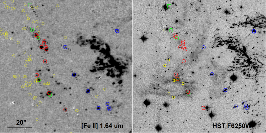
Figure 15: Distribution of optical NKs (yellow circles) in the catalog of Hammell & Fesen (2008) shown on the deep [Fe II] and HST F625W images. North is up, and east is to the left. The circles/squares and their colors are the same as in Figure 14. The black bars in the deep [Fe II] image represent the locations of the 10″-long MOS slits. In the F6250W image, only the bright NK knots with an F6250W flux larger than $6\times 10^{-17}$ erg cm² s^-1 are shown. Note that the positions of the slit and knot symbols are shifted to the epochs of the background images, i.e., 2013 Sept. for the deep [Fe II] image and 2004 Mar. for the HST image.

We detected seven knots that show only He I 1.083 µm lines. The He I 1.083 µm line intensities of these He I knots are not particularly strong in comparison with other metal-rich ejecta knots (Figure 5). But, since [Fe II] 1.257 µm line is not detected, they are noticeable by their very high $R$(He I/[Fe II]), which is 1–2 orders of magnitude higher than the typical S-rich and Fe-rich ejecta knots (see the bottom frame of Figure 4). Table 7 lists the knots with $R$(He I/[Fe II]) greater than 8 where we can see that the majority are He I knots.

He I knots are detected along the forward shock front, from the southern base of the NE jet to the Fe K plume area (see Figure 6). The radial velocities of He I knots are spread over a very wide range, from $-3300~{}{\rm km~{}s}^{-1}$ to $+3200~{}{\rm km~{}s}^{-1}$ (Figure 8 and Table 7). Since most of them have very high radial velocities, they are probably not circumstellar material. Their spectral properties are also different from the low-velocity circumstellar clumps in Cas A, which are called quasi-stationary flocculi (QSFs). QSFs are He and N-enriched circumstellar material ejected by the progenitor before SN explosion and have been shocked by the SN blast wave recently (Peimbert & van den Bergh 1971; McKee & Cowie 1975; see also Koo et al. 2023 and references therein). In NIR, QSFs show strong He I lines together with moderately strong [Fe II] and [S II] lines and also weak Pa$\gamma$ and [C I] 0.985 µm lines (Chevalier & Kirshner, 1978; Gerardy & Fesen, 2001; Lee et al., 2017). The ratio of Pa$\gamma$ to He I 1.083 µm is typically $\sim 0.03$ (see Koo et al. 2023). For comparison, all He I knots show strong ($>10^{-15}$ erg cm^-2 s^-1) He I lines without [Fe II] or [S II] lines, and about half of them also show weak [C I] 0.985 µm line.

What’s the origin of He I knots? The first possibility that we can consider is that they are debris of the He-rich envelope material of the progenitor star expelled by the SN explosion, like high-velocity N-rich knots (NKs) detected in optical studies (Fesen et al., 1987, 1988; Fesen & Becker, 1991; Fesen, 2001; Hammell & Fesen, 2008; Fesen & Milisavljevic, 2016). The spectra of NKs are dominated by strong [N II] $\lambda\lambda$6548, 6583 lines in the wavelength region 4500–7200 Å. For most NKs, H$\alpha$ line is either much weaker than [N II] lines or undetected, so NKs are considered as important evidence that the Cas A progenitor had a thin N-rich and H-poor envelope at the time of SN explosion. A deep, ground-based [N II] imaging observations detected 50 NKs, whereas HST observations revealed numerous NKs distributed around the remnant. In particular, in the eastern area where He I knots have been detected, many NKs had been detected (Figure 15; see also Figure 5 of Fesen 2001 or Figure 9E of Fesen & Milisavljevic 2016). The radial velocities of the bright NK knots in the eastern area are in the range of $-2000$ to +2500 ${\rm km~{}s}^{-1}$ (Fesen, 2001). So the association of He I knots with NKs seems plausible considering that He abundance might be enhanced in the CNO-processed, N-rich envelope of the progenitor star. Apparently, however, none of the He I knots has an optical NK counterpart (Table 7; see § 4.3). Another difficulty in connecting He I knots to NKs is the non-detection of He I $\lambda$5876 line in NKs (Fesen & Becker, 1991; Fesen, 2001). The recombination emissivity of He I $\lambda$5876 line is a factor of 2–10 smaller than that of He I 1.083 µm line depending on electron density ($10^{2}$–$10^{4}$ cm^-3) in the Case B approximation (e.g., Draine, 2003). The flux will be further reduced by interstellar extinction. Hence, He I $\lambda$5876 line is expected to be much weaker than He I 1.083 µm line, but it is not obvious if that can explain the non-detection of He I $\lambda$5876 lines. An interesting possibility is that the He I knots originated from the lower portion of the He-rich envelope of the progenitor star where N is depleted. If a large amount of carbon is dredge-up by convection, nitrogen could be depleted because ¹⁴N mixed into the lower layer by convection participates the ${}^{14}\mathrm{N}(\alpha,\gamma)^{18}\mathrm{F}(\beta^{+})^{18}\mathrm{O}(\alpha,\gamma)^{22}\mathrm{Ne}$ reaction. Such a ¹⁴N-depleted region formed by convective dredge-up is often found at the pre-SN stage in massive star models (Y. Jung et al, in preparation). Observationally, our slits are positioned toward [Fe II] line-emitting knots by design. So it is possible that we are picking up He-rich, N-depleted knots that are located closer to the explosion center than the optical NKs, but which coincidentally overlap with the same region of sky as the Fe-emitting knots (Figure 15). Future studies may further explore the possibility.

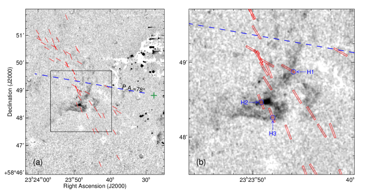
Figure 16: (a) Continuum-subtracted H$\alpha$ image of the eastern area of Cas A. The symbols and lines are the same as in Figure 1. (b) An enlarged view of the boxed area in (a). The blue circles represent the central positions of the H emission features: H1, H2, and H3 in Table 8. The image has been produced from the Isaac Newton Telescope (INT) Wide Field Survey (WFS) data obtained in 2005 October.

Another possibility is that they are metal-enriched SN ejecta with relatively high He abundance. We note that some S-rich and Fe-rich knots have very high $R$(He I/[Fe II]), as high as the He I knots, and that the majority of He I knots have [S II] 1.03 µm and [C I] 0.985 µm flux upper limits that are not particularly strong (Table 7). This explanation also appears to be consistent with that the half of He knots seem to be FMK-like knots in optical classifications (Figure 11). The overabundance of low atomic elements could be attributed to significant mixing among the nucleosynthetic layers as pointed out in previous X-ray and optical studies (Fesen & Becker, 1991; Fesen & Gunderson, 1996). From optical spectroscopy, Fesen & Becker (1991) reported the detection of a hybrid ejecta knot showing O and S emission lines along with [N II] and H$\alpha$ emission lines in the NE jet region, and they called it a ‘mixed emission knot’ (MEK). Additional optical studies towards the outer region of the remnant have further detected several MEKs, which suggested chemical mixing among the nucleosynthetic layers between the explosive O-burning layer and the N-rich photospheric envelop of the progenitor (Fesen & Gunderson, 1996; Fesen, 2001). Yet another possibility is that He I knots are the remains of the complete Si burning with $\alpha$-rich freezeout in the innermost region of the progenitor as helium in Fe-rich knots (see also Lee et al., 2017). But it seems to be difficult for this scenario to explain the difference in radial velocities between the He I knots and the Fe-rich knots.

It is also worth noticing that Figure 6 does not represent the overall distribution of He I knots. Since our observation was done toward ejecta knots bright in [Fe II] emission, the detection of He I knots was unexpected. He I knots were detected because they fell on the slit by chance. In order to see the overall distribution He I knots, which is essential for understanding their origin, we need He I 1.083 µm narrow-band observations of the Cas A remnant.

5.4 Extended H emission Features Associated with East Cloud

In addition to the 67 SN ejecta knots, we also detected three “extended H emission features” in the outer eastern region (Section 3), and their physical properties are listed in Table 8. They show only unresolved (FWHM $\lower 2.15277pt\hbox{$\;\buildrel<\over{\sim}\;$}9$ Å) H I lines, e.g., Pa$\gamma$ 1.094 µm and Pa$\beta$ 1.282 µm lines, without any emission lines from metallic elements, and have radial velocities between $-20$ ${\rm km~{}s}^{-1}$ and $-30~{}{\rm km~{}s}^{-1}$, indicating that they are of CSM/ISM origin. We can estimate the line-of-sight extinction to the H-emitting gas using the flux ratio of H I emission lines. All three features show Pa$\beta$ line, and the brightest one (H2) also shows Pa$\gamma$ line. The observed H I line ratio, $F$(Pa$\gamma$)/$F$(Pa$\beta$), is $0.41\pm 0.09$. By comparing with the unreddened line ratio of 0.56 at $T_{\rm e}=10^{4}$ K and $n_{\rm e}=10^{4}$ cm^-3 (Hummer & Storey, 1987), we obtained $N_{\rm H}$ of $7.6^{+6.4}_{-5.1}\times 10^{21}$ cm^-2 which is corresponding to $A_{\rm V}$ of $4.1^{+3.4}_{-2.7}$ mag. The extinction-corrected $F$([Fe II] 1.257)/$F$(Pa$\beta$) is $<0.2$ ($2\sigma$ upper limit), which is at least an order of magnitude smaller than that in the typical shock-excited CSM/ISM detected in the several Galactic SNRs (2–20; Koo & Lee, 2015, and references therein). This low $F$([Fe II] 1.257)/$F$(Pa$\beta$) indicates that the H I lines are associated with a photoionized gas.

We noticed that the positions of the extended H emission features are coincident with the region where a bright, diffuse optical cloud is detected (Figure 16). The diffuse cloud in the eastern region (hereafter “East Cloud”), located 2$\farcm$7 east from the center of the remnant, was first identified in an early optical photograph taken by R. Minkowski (Minkowski, 1968; van den Bergh, 1971), and it has a triangular shape with a size of $\sim 1\arcmin$ (see also the right panel of Figure 16). In a deep H$\alpha$ narrow-band image, however, it turned out to be more extended and diffuse (see Figure 10 in Fesen 2001 or Figure 2 in Weil et al. 2020). The follow-up optical spectroscopy showed that the East Cloud emits strong H$\alpha$ emission line accompanied by relatively weak [O III] $\lambda\lambda$ 4959, 5007, [N I] $\lambda\lambda$ 6548, 6583, and [S II] $\lambda\lambda$ 6716, 6725 lines (Fesen et al., 1987; Weil et al., 2020).

The origin of the East Cloud as well as its physical association with Cas A has been controversial. The early optical studies suggested that it is a small, diffuse H II region adjacent to the remnant (Minkowski, 1968; van den Bergh, 1971). However, the lack of OB stars around the eastern cloud suggested that it is a diffuse CSM/ISM nearby Cas A excited by the UV/X-ray emission from the SN outburst (Peimbert, 1971; van den Bergh, 1971; Weil et al., 2020). In this scenario, the East Cloud could be either the diffuse ISM surrounding the progenitor star (Minkowski, 1968; van den Bergh, 1971; Peimbert & van den Bergh, 1971; Peimbert, 1971) or the diffuse CSM blown out from the progenitor star during its red supergiant phase (Fesen et al., 1987; Chevalier & Oishi, 2003; Weil et al., 2020). The peculiar structure of the East Cloud, its projected proximity to the NE jet, and distinct spectroscopic properties relative to the surrounding diffuse emissions are indirect evidence suggesting the physical association of the East Cloud with the remnant (Fesen et al., 1987; Fesen & Gunderson, 1996; Fesen et al., 2006; Weil et al., 2020), while the presence of brightened ejecta knots matching the East Cloud’s emission structure provides strong evidence that the East Cloud is physically adjacent to Cas A (Weil et al., 2020).

According to our spectroscopy, the mean $v_{\rm LSR}$ of the Pa$\beta$ lines weighted by 1/$\sigma_{v}^{2}$ (where $\sigma_{v}$ is the $1\sigma$ uncertainty of the central velocity) is $-22\pm 5~{}{\rm km~{}s}^{-1}$ (see Table 8). Considering the systematic uncertainty from the wavelength calibration ($\sim 12~{}{\rm km~{}s}^{-1}$; see Section 2), the $v_{\rm LSR}$ of the East Cloud is $-22\pm 13~{}{\rm km~{}s}^{-1}$. This is consistent with the previous result: $v_{\rm LSR}=-20\pm 75~{}{\rm km~{}s}^{-1}$ from a few bright optical lines (Fesen et al., 1987) and $v_{\rm LSR}=-13\pm 10~{}{\rm km~{}s}^{-1}$ from H$\alpha$ lines (Alarie et al., 2014). Previous radio observations, however, showed that Cas A is located at the far-side of the Perseus spiral arm implying $v_{\rm LSR}\sim-50~{}{\rm km~{}s}^{-1}$ for Cas A (Zhou et al., 2018b, and references therein). Furthermore, recent NIR observations for the southern optical QSF (“Knot 24”) reported the detection of narrow (${\rm FWHM}\sim 8~{}{\rm km~{}s}^{-1}$) [Fe II] lines from unshocked pristine CSM with $v_{\rm LSR}\simeq-50~{}{\rm km~{}s}^{-1}$ (Koo et al., 2020), which is consistent with the systematic velocity center $v_{\rm LSR}\simeq-50~{}{\rm km~{}s}^{-1}$ of Cas A. So the velocity of the East Cloud ($v_{\rm LSR}\sim-22~{}{\rm km~{}s}^{-1}$) is considerably different from the systemic velocity of the Cas A SNR. This might indicate that the East Cloud is not physically associated with the remnant, but is located at $\sim 2$ kpc from us (more than 1 kpc closer than the remnant) assuming the flat Galactic rotation model with IAU standard ($R_{0}=8.5$ kpc and $v_{0}=220~{}{\rm km~{}s}^{-1}$). Relatively low line-of-sight extinction of the East Cloud ($A_{\rm V}\sim 4$ mag) derived from their H I lines compared to that toward the remnant ($A_{\rm V}=6$–$10$ mag; see Figure 2) seems to support this possibility. On the other hand, if the East Cloud is the CSM material ejected from the progenitor star as suggested by Chevalier & Oishi (2003) and Weil et al. (2020), the velocity difference ($\sim 30~{}{\rm km~{}s}^{-1}$) should represent the line-of-sight component of the ejection velocity of the CSM. And, considering that the East Cloud is located at the eastern outer edge of the remnant, the ejection velocity should have been much higher than $30$ ${\rm km~{}s}^{-1}$, or than the typical wind velocity of red supergiant stars, e.g., $10$–$20~{}{\rm km~{}s}^{-1}$ (Smith, 2014).

6 Summary

The Cas A SNR has a quite complex structure, manifesting the violent and asymmetric explosion. Two representative features are the NE jet and the Fe K plume in the outer eastern area of the SNR. The NE jet is a stream of ejecta material dominated by intermediate mass elements beyond the SN blast wave, and the Fe K plume is a plume of X-ray emitting hot gas dominated by Fe ejecta outside the main ejecta shell. These two features are expanding much faster than the main ejecta shell of the SNR, suggesting turbulent convection and hydrodynamic instabilities in the early stages of the SN explosion. We carried out NIR (0.95–1.75 µm) MOS spectroscopy of the NE jet and Fe K plume regions of the Cas A SNR using MMIRS. In the two-dimensional spectra of 52 MOS slits, which were positioned on the bright knots in the deep [Fe II] 1.64 $\mu$m image of Koo et al. (2018), a total of 67 knots have been identified. All knots show at least one of the following strong lines: [S III] 0.983 $\mu$m, He I 1.083 $\mu$m, [S II] 1.03 $\mu$m, and [Fe II] 1.257 $\mu$m lines. And about one third of the knots also show strong [P II] 1.189 $\mu$m line. We find that the knots in different areas show distinctively different ratios of these lines, suggesting their different elemental composition. The NIR lines are emitted from shocked gas, so their intensities depend on shock environments as well as the elemental composition of the knots, e.g., density and velocity of the knots, density contrast between the knot and the ambient gas, ambient pressure. In metal rich ejecta knots, the elemental composition also profoundly affects the cooling function and therefore the physical structure of the shocked gas (e.g., Raymond, 2019). Hence, it would be a formidable task to derive the elemental composition from just the NIR spectra. In this work, we simply classify the knots into three groups based on the relative strengths of [S II], [Fe II], and He I lines, i.e., S-rich, Fe-rich, and He I knots, and explore the origins of these knots and their connection to the explosion dynamics of the Cassiopeia A supernova. We summarize our main results as follows.

1. The NE jet is dominated by S-rich knots. There are no Fe-rich knots without [S II] lines. The knots show weak or no [P II] lines, which clearly differentiates them from the S-rich ejecta in the main ejecta shell that have strong [P II] lines. The low P abundance inferred from their low [P II]/[Fe II] line ratios indicate that these S-rich knots were produced below the explosive Ne burning layer, which is consistent with the results of previous studies. Our results do not support the jet-induced explosion model, but it is also not clear if the NE jet can be explained by the neutrino-driven explosion model.

2. In the Fe K plume area, along the forward shock front just outside the boundary of the diffuse X-ray emitting Fe ejecta, we detected Fe-rich knots showing only [Fe II] lines with or without He I line. These NIR Fe-rich ejecta knots are expanding with velocities considerably higher than the X-ray Fe ejecta. The spatial and kinematic relations support the physical association of these dense NIR Fe-rich knots with the X-ray diffuse Fe ejecta produced by explosive complete Si burning with $\alpha$ freezeout. We suggest that the initial density distribution of the Fe ejecta produced in the innermost region was very inhomogeneous and that the dense knots were ejected with the diffuse Fe ejecta but decoupled after crossing the reverse shock.

3. We also detected several He I knots emitting only He I 1.083 µm lines with or without very weak [C I] 0.985 $\mu$m lines. They are detected along the forward shock front from the southern base of the NE jet to the Fe K plume area. The origin of these He-rich knots is unclear. They are likely the debris of the He-rich layer above the carbon-oxygen core of the progenitor expelled during the SN explosion, but they could be also metal-enriched SN ejecta with relatively high He abundance or the remains of the explosive complete Si burning in $\alpha$-rich freezeout. The detection of He I knots was unexpected because our MMT observations were directed toward ejecta knots bright in [Fe II] emission. So an imaging observation is needed to reveal the distribution of He I knots.

4. In addition to the 67 SN ejecta knots, we also detected three extended H emission features associated with the diffuse cloud, the East Cloud, in the eastern area well beyond the SNR boundary. They show only narrow H recombination lines with low line of sight velocities ($\sim-20$ ${\rm km~{}s}^{-1}$), indicating that the lines are arising from photoionized CSM/ISM. Their velocities are substantially different from the systematic velocity of the Cas A ($v_{\rm LSR}\sim-50$ ${\rm km~{}s}^{-1}$), and it implies that, if the East Cloud is a CSM ejected from the progenitor star of the Cas A SN, the ejection velocity should have been much higher than 30 ${\rm km~{}s}^{-1}$ considering its location.

Table 1: Log of MOS Spectroscopy

Mask	Number of Slits	Grism	Filter	P.A.	Exposure Time
				(degree)	(sec)
MASK 1	20	J	zJ	32	$300\times 8$
		H3000	H	32	$300\times 4$
MASK 2	17	J	zJ	21	$300\times 12$
MASK 3	15	J	zJ	60	$300\times 12$

Note. — (1) mask name; (2) number of MOS slits in each mask; (3) grism; (4) filter; (5) position angle of slits measured counterclockwise from north to east on the plane of the sky; (6) exposure time per frame (sec) $\times$ number of dithering.

Table 2: Slit Positions

Mask	Slit No.	$\alpha(J2000)$	$\delta(J2000)$	Mask	Slit No.	$\alpha(J2000)$	$\delta(J2000)$
MASK 1	05	23:24:00.342	+58:51:06.45	MASK 3	07	23:23:59.854	+58:50:50.70
	06	23:23:59.797	+58:50:53.89		08	23:23:58.676	+58:50:42.03
	07	23:23:57.769	+58:50:49.28		09	23:23:57.739	+58:50:31.51
	08	23:23:54.621	+58:50:50.54		10	23:23:55.808	+58:50:35.53
	09	23:23:55.148	+58:50:32.56		11	23:23:56.335	+58:50:05.89
	10	23:23:52.626	+58:50:22.26		12	23:23:54.448	+58:50:07.00
	11	23:23:48.962	+58:50:26.84		13	23:23:51.720	+58:50:21.20
	12	23:23:52.200	+58:49:57.42		14	23:23:52.053	+58:49:53.03
	13	23:23:50.194	+58:49:40.02		15	23:23:48.541	+58:50:00.63
	14	23:23:49.642	+58:49:24.08		16	23:23:50.035	+58:49:09.96
	15	23:23:49.462	+58:49:04.85		17	23:23:48.548	+58:48:59.68
	16	23:23:48.859	+58:48:54.93		18	23:23:46.346	+58:48:54.93
	17	23:23:48.487	+58:48:43.22		19	23:23:40.964	+58:49:08.44
	18	23:23:45.436	+58:48:32.51		22	23:23:38.661	+58:48:22.95
	19	23:23:43.979	+58:48:19.23		23	23:23:37.549	+58:48:13.42
	20	23:23:42.877	+58:48:05.38
	21	23:23:38.578	+58:48:12.57
	22	23:23:43.680	+58:47:33.33
	24	23:23:38.731	+58:47:29.37
	28	23:23:37.742	+58:46:34.72
MASK 2	03	23:23:52.229	+58:51:39.22
	04	23:23:56.865	+58:51:07.09
	05	23:23:56.026	+58:50:48.34
	06	23:23:55.432	+58:50:34.78
	07	23:23:49.371	+58:50:31.02
	08	23:23:50.915	+58:50:12.42
	09	23:23:51.953	+58:49:55.88
	10	23:23:50.194	+58:49:40.02
	12	23:23:49.296	+58:49:03.66
	13	23:23:48.340	+58:48:53.28
	14	23:23:49.155	+58:48:28.37
	15	23:23:48.034	+58:48:17.59
	16	23:23:46.344	+58:48:04.12
	17	23:23:41.761	+58:48:05.40
	18	23:23:44.543	+58:47:31.34
	19	23:23:40.775	+58:47:28.46
	23	23:23:42.721	+58:46:19.80

Table 3: Physical Parameters of 67 Ejecta Knots

Knot No.	ID	$\alpha$(J2000)	$\delta$(J2000)	P.A.	$d_{\rm rad}$	FWHM	$v_{\rm rad}$	$N_{\rm H}$	Knot	K2018 No.
				($\arcdeg$)	($\arcmin$)	(${\rm km~{}s}^{-1}$)	(${\rm km~{}s}^{-1}$)	($10^{22}$ cm-2)	Type
1	2-07-2	23:23:49.49	+58:50:33.4	58.3	3.30	277 ( 8)	$+2336~{}(2)$	1.42	S	169B
2	2-04-1	23:23:56.87	+58:51:07.1	58.6	4.41	292 (34)	$+420~{}(15)$	1.85	S	182
3	2-07-1	23:23:49.37	+58:50:31.0	58.7	3.27	298 ( 2)	$+141~{}(1)$	1.42	S	169A
4	1-11-1	23:23:48.96	+58:50:26.8	59.3	3.19	318 ( 6)	$+272~{}(3)$	1.41	S	168
5	1-08-1	23:23:54.62	+58:50:50.5	59.8	4.02	249 ( 1)	$+124~{}(1)$	1.60	S	180
6	1-05-2	23:24:00.52	+58:51:08.7	61.2	4.83	247 (26)	$+172~{}(11)$	1.75	S	$\cdots$
7	2-05-1	23:23:56.03	+58:50:48.3	61.5	4.16	214 (16)	$+428~{}(7)$	1.74	S	181
8	1-05-1	23:24:00.34	+58:51:06.5	61.5	4.79	264 (19)	$+748~{}(9)$	1.72	S	184
9	1-07-1	23:23:57.77	+58:50:49.3	62.7	4.37	297 (17)	$+832~{}(10)$	1.88	S	200
10	1-06-2	23:24:00.19	+58:50:58.8	62.7	4.72	174 (11)	$+452~{}(4)$	1.77	S	$\cdots$
11	1-06-1	23:23:59.80	+58:50:53.9	63.3	4.63	286 ( 3)	$+10~{}(2)$	1.73	S	207
12	3-13-1	23:23:51.72	+58:50:21.2	63.7	3.46	248 ( 5)	$+429~{}(3)$	1.55	S	188
13	2-06-1	23:23:55.43	+58:50:34.8	63.8	3.99	339 ( 7)	$+541~{}(4)$	1.58	S	195A
14	3-10-1	23:23:55.81	+58:50:35.5	64.0	4.04	369 ( 9)	$+519~{}(4)$	1.61	S	195B
15	3-07-1	23:23:59.85	+58:50:50.7	64.0	4.62	311 ( 7)	$+110~{}(4)$	1.73	S	206
16	1-09-1	23:23:55.15	+58:50:32.6	64.1	3.94	227 ( 8)	$+483~{}(3)$	1.58	S	194
17	1-10-1	23:23:52.62	+58:50:22.3	64.3	3.57	283 ( 3)	$+490~{}(2)$	1.66	S	189
18	3-08-1	23:23:58.68	+58:50:42.0	64.8	4.42	245 (28)	$+625~{}(10)$	1.73	S	201
19	2-08-1	23:23:50.92	+58:50:12.4	65.2	3.30	421 (61)	$+799~{}(26)$	1.49	S	187A
20	2-08-2	23:23:50.90	+58:50:12.0	65.2	3.29	271 (39)	$-230~{}(17)$	1.49	S	187B
21	3-15-2	23:23:49.10	+58:50:03.1	66.0	3.02	312 (28)	$+329~{}(14)$	1.46	S	$\cdots$
22	3-15-1	23:23:48.54	+58:50:00.6	66.1	2.94	441 (16)	$+2485~{}(8)$	1.46	S	$\cdots$
23	3-09-1	23:23:57.74	+58:50:31.5	66.3	4.24	227 (10)	$-234~{}(4)$	1.66	Fe	197
24	3-12-1	23:23:54.45	+58:50:07.0	69.4	3.69	302 ( 6)	$-696~{}(3)$	1.64	S	220
25	1-12-1	23:23:52.20	+58:49:57.4	70.2	3.36	252 ( 3)	$-600~{}(2)$	1.65	S	214A
26	1-12-3	23:23:52.16	+58:49:56.9	70.3	3.35	241 (15)	$+3242~{}(8)$	1.65	He	$\cdots$
27	2-09-1	23:23:51.95	+58:49:55.9	70.5	3.32	317 ( 6)	$-515~{}(2)$	1.65	S	214B
28	3-11-1	23:23:56.34	+58:50:05.9	70.9	3.91	304 (11)	$-1199~{}(5)$	1.62	S	224
29	1-12-2	23:23:51.87	+58:49:53.3	71.1	3.30	256 (11)	$-2116~{}(6)$	1.65	S	$\cdots$
30	3-11-2	23:23:55.84	+58:50:03.7	71.1	3.84	247 ( 9)	$+752~{}(4)$	1.62	S	222
31	3-14-1	23:23:52.05	+58:49:53.0	71.3	3.32	281 ( 3)	$-2125~{}(2)$	1.65	S	212
32	3-14-2	23:23:51.78	+58:49:51.8	71.4	3.28	217 ( 8)	$-3170~{}(4)$	1.62	S	$\cdots$
33	2-09-2	23:23:51.72	+58:49:51.2	71.6	3.27	249 ( 9)	$-3152~{}(3)$	1.62	He	$\cdots$
34	1-13-1	23:23:50.19	+58:49:40.0	73.8	3.02	250 ( 8)	$-2017~{}(4)$	1.49	S	226
35	1-14-2	23:23:50.05	+58:49:29.2	77.0	2.96	187 (10)	$+2314~{}(6)$	1.48	He	$\cdots$
36	3-19-1	23:23:40.96	+58:49:08.4	79.5	1.74	358 (35)	$-1954~{}(14)$	1.57	S	229
37	3-19-2	23:23:40.90	+58:49:08.1	79.6	1.73	286 (22)	$-2411~{}(9)$	1.57	S	$\cdots$
38	3-16-2	23:23:49.86	+58:49:09.2	83.4	2.88	211 (14)	$-3312~{}(6)$	1.47	He	$\cdots$
39	1-15-1	23:23:49.46	+58:49:04.9	84.7	2.82	247 (13)	$-1286~{}(5)$	1.42	Fe	235
40	2-12-1	23:23:49.30	+58:49:03.7	85.1	2.80	268 (13)	$-1282~{}(5)$	1.42	Fe	234
41	2-12-2	23:23:49.23	+58:49:02.4	85.5	2.79	271 (23)	$-269~{}(11)$	1.42	He	$\cdots$
42	3-17-1	23:23:48.55	+58:48:59.7	86.3	2.70	210 (17)	$-1616~{}(8)$	1.39	Fe	232
43	2-13-3	23:23:48.58	+58:48:58.1	86.9	2.70	259 (17)	$-1987~{}(5)$	1.39	Fe	$\cdots$
44	3-18-1	23:23:46.35	+58:48:54.9	87.8	2.41	261 (14)	$-1319~{}(6)$	1.47	S	238
45	2-13-2	23:23:48.42	+58:48:55.0	88.0	2.68	235 ( 8)	$-1165~{}(3)$	1.37	Fe	$\cdots$
46	1-16-1	23:23:48.86	+58:48:54.9	88.0	2.73	242 ( 3)	$-1189~{}(2)$	1.39	Fe	241
47	2-13-1	23:23:48.34	+58:48:53.3	88.6	2.66	328 ( 4)	$-1159~{}(2)$	1.37	Fe	239
48	1-17-1	23:23:48.49	+58:48:43.2	92.2	2.68	161 (14)	$-903~{}(6)$	1.37	Fe	240
49	2-14-2	23:23:49.34	+58:48:32.1	95.9	2.81	227 (17)	$-1554~{}(9)$	1.34	Fe	251
50	1-18-1	23:23:45.44	+58:48:32.5	97.0	2.30	273 ( 3)	$+755~{}(2)$	1.44	S	244
51	2-14-1	23:23:49.15	+58:48:28.4	97.2	2.79	257 ( 6)	$-207~{}(2)$	1.32	Fe	250
52	2-14-3	23:23:49.14	+58:48:28.2	97.2	2.79	246 ( 2)	$+765~{}(1)$	1.32	He	$\cdots$
53	2-15-1	23:23:48.03	+58:48:17.6	101.4	2.68	303 (10)	$-644~{}(4)$	1.36	Fe	259
54	2-15-2	23:23:47.96	+58:48:16.1	102.0	2.67	257 ( 2)	$+1187~{}(1)$	1.36	He	$\cdots$
55	1-19-1	23:23:43.98	+58:48:19.2	103.4	2.16	349 ( 9)	$+753~{}(5)$	1.41	S	270
56	2-16-1	23:23:46.34	+58:48:04.1	107.4	2.52	230 (11)	$-1413~{}(6)$	1.41	Fe	272
57	2-17-2	23:23:41.93	+58:48:08.8	110.3	1.95	280 (15)	$-2052~{}(7)$	1.43	S	$\cdots$
58	1-20-1	23:23:42.88	+58:48:05.4	110.5	2.09	290 ( 7)	$-1651~{}(4)$	1.39	S	277
59	2-17-1	23:23:41.76	+58:48:05.4	112.0	1.95	320 (35)	$-531~{}(14)$	1.42	S	275
60	2-17-3	23:23:41.70	+58:48:04.3	112.6	1.95	405 (37)	$+560~{}(18)$	1.46	S	$\cdots$
61	3-23-1	23:23:37.55	+58:48:13.4	115.3	1.40	375 ( 5)	$-674~{}(3)$	1.68	S	282
62	3-23-2	23:23:37.33	+58:48:12.4	116.5	1.38	300 ( 8)	$-4004~{}(5)$	1.69	S	281
63	2-18-1	23:23:44.54	+58:47:31.3	120.9	2.53	280 (22)	$-2023~{}(10)$	1.48	Fe	290
64	1-22-1	23:23:43.68	+58:47:33.3	121.6	2.42	274 (40)	$-1725~{}(21)$	1.47	Fe	288
65	2-19-1	23:23:40.78	+58:47:28.5	128.7	2.16	339 (13)	$-44~{}(7)$	1.42	S	293
66	1-24-1	23:23:38.73	+58:47:29.4	133.2	1.95	436 (24)	$+46~{}(13)$	1.43	S	296
67	2-23-1	23:23:42.72	+58:46:19.8	142.1	3.16	197 ( 3)	$+1957~{}(2)$	1.44	Fe	299

Note. — (1) knot serial number in this work; (2) Mask-Slit-number, where the number is the serial number of a knot detected in the slit; (3)–(4) coordinate of the emission feature in the slit; (5) position angle measured counterclockwise from north to east at the center of the SN explosion; (6) radial distance from the center of the SN explosion; (7)–(8) FWHM and central LSR velocity of the knot obtained from a weighted average of the emission lines. The numbers in the parentheses are the $1\sigma$ statistical uncertainties from single Gaussian fittings (see § 2); (9) hydrogen column density derived from an Herschel SPIRE 250 µm image; (10) knot type: S = S-rich knot, Fe = Fe rich knot, He=He I knot. See § 4.2 for an explanation about the classification of the knots.; (11) Knot serial number in Koo et al. (2018).

Table 4: Observed NIR Line Parameters of 67 Ejecta Knots

Knot	Line ID	$\lambda_{\rm rest}$	Observed Flux
No.	Transition ($l$–$u$)	($\micron$)	($10^{-17}$ erg s-1 cm-2)
1	[S III]   ${}^{3}P_{2}$ – ${}^{1}D_{2}$	0.95337	21.9 ( 2.8)
1	[C I]     ${}^{3}P_{1}$ – ${}^{1}D_{2}$	0.98268	$\cdot$ ( 2.4)
1	[C I]     ${}^{3}P_{2}$ – ${}^{1}D_{2}$	0.98530	11.5 ( 1.7)
1	[S II]    ${}^{2}D_{3/2}$ – ${}^{2}P_{3/2}$	1.02896	15.0 ( 0.8)
1	[S II]    ${}^{2}D_{5/2}$ – ${}^{2}P_{3/2}$	1.03233	18.2 ( 0.0)
1	[S II]    ${}^{2}D_{3/2}$ – ${}^{2}P_{1/2}$	1.03392	11.3 ( 1.3)
1	[S II]    ${}^{2}D_{5/2}$ – ${}^{2}P_{1/2}$	1.03733	4.9 ( 0.0)
1	[S I]     ${}^{3}P_{2}$ – ${}^{1}D_{2}$	1.08241	14.8 ( 2.0)
1	He I      ${}^{3}S_{1}$ – ${}^{3}P_{0,1,2}$	1.08332	257.0 ( 5.0)
1	[S I]     ${}^{3}P_{1}$ – ${}^{1}D_{2}$	1.13089	$\cdot$ ( 0.7)
1	[P II]    ${}^{3}P_{2}$ – ${}^{1}D_{2}$	1.18861	$\cdot$ ( 1.0)
1	[Fe II]   $a^{6}D_{7/2}$ – $a^{4}D_{5/2}$	1.24888	$\cdot$ (21.3)
1	[Fe II]   $a^{6}D_{3/2}$ – $a^{4}D_{1/2}$	1.25248	$\cdot$ ( 2.4)
1	[Fe II]   $a^{6}D_{9/2}$ – $a^{4}D_{7/2}$	1.25702	5.9 ( 1.8)
1	[Fe II]   $a^{6}D_{1/2}$ – $a^{4}D_{1/2}$	1.27069	$\cdot$ ( 3.3)
1	[Fe II]   $a^{6}D_{3/2}$ – $a^{4}D_{3/2}$	1.27913	$\cdot$ ( 2.1)
1	[Fe II]   $a^{6}D_{5/2}$ – $a^{4}D_{5/2}$	1.29462	$\cdot$ ( 2.4)
1	[Fe II]   $a^{6}D_{1/2}$ – $a^{4}D_{3/2}$	1.29813	$\cdot$ ( 4.5)
1	[Fe II]   $a^{6}D_{7/2}$ – $a^{4}D_{7/2}$	1.32092	$\cdot$ ( 1.2)
1	[Fe II]   $a^{6}D_{3/2}$ – $a^{4}D_{5/2}$	1.32814	$\cdot$ ( 0.9)
1	[Fe II]   $a^{4}F_{9/2}$ – $a^{4}D_{5/2}$	1.53389	$\cdot$($\cdot$)
1	[Fe II]   $a^{4}F_{7/2}$ – $a^{4}D_{3/2}$	1.59991	$\cdot$($\cdot$)
1	[Si I]    ${}^{3}P_{1}$ – ${}^{1}D_{2}$	1.60727	$\cdot$($\cdot$)
1	[Fe II]   $a^{4}F_{9/2}$ – $a^{4}D_{7/2}$	1.64400	$\cdot$($\cdot$)
1	[Si I]    ${}^{3}P_{2}$ – ${}^{1}D_{2}$	1.64590	$\cdot$($\cdot$)
1	[Fe II]   $a^{4}F_{5/2}$ – $a^{4}D_{1/2}$	1.66422	$\cdot$($\cdot$)
1	[Fe II]   $a^{4}F_{7/2}$ – $a^{4}D_{5/2}$	1.67733	$\cdot$($\cdot$)
1	[Fe II]   $a^{4}F_{5/2}$ – $a^{4}D_{3/2}$	1.71159	$\cdot$($\cdot$)
1	[Fe II]   $a^{4}F_{3/2}$ – $a^{4}D_{1/2}$	1.74541	$\cdot$($\cdot$)

Note. — (1) knot serial number in this work; (2) line ID and its transition; (3) rest wavelength in vacuum; (4) observed line flux. The numbers in the parentheses are the $1\sigma$ statistical uncertainties from single Gaussian fittings (see S 2).

Note. — This table is available in its entirety in a machine-readable form in the online journal.

Table 5: Spectral Classification of the 67 NIR Ejecta Knots and their Statistics

Knot Group	Spectral Properties	Number of Knots
		NE jet area	Fe K plume area
S-rich Knots	strong [S II], [Fe II] lines	31	13
	strong [P II] line (Fe K plume area); weak/no [P II] line (NE jet area)
	$R$([S II]/[Fe II]) $>3.7$
Fe-rich Knots	strong [Fe II] line; weak or no [S II], [P II] lines	1	15
	$R$([S II]/[Fe II]) $<3.7$
He I Knots	strong He I line; weak or no [C I] line	3	4
	$R$(He I/[Fe II]) $>8$
Total		35	32

Note. — (1) knot group; (2) line ratios; (3)–(4) number of knots in the NE jet and Fe K plume areas

Table 6: Properties of Fe-rich Knots

Knot	K2019 No	$\alpha$(J2000)	$\delta$(J2000)	Size	$\mu$	$F_{{\rm[Fe\,II]}1.644\,\mu{\rm m}}$	$v_{r}$	${F({\rm[S\,II]})\over F({\rm[Fe\,II]})}$	${F({\rm[P\,II]})\over F({\rm[Fe\,II]})}$	${F({\rm He\,I})\over F({\rm[Fe\,II]})}$	Optical
No				(arcsec)	(km s-1)	(erg cm-2 s-1)	(km s-1)				Counterpart
23	197	23:23:57.399	58:50:30.36	2.26$\times$1.44	$\cdots$	5.75E-16	-234	1.78	$\leq$0.13	$\leq$0.26	FMK
39	235	23:23:49.208	58:49:04.65	1.85$\times$1.48	$\cdots$	4.66E-16	-1286	$\leq$1.72	$\leq$0.10	0.71	FMK
40	234	23:23:49.044	58:49:03.51	1.69$\times$1.44	$\cdots$	5.17E-16	-1282	$\leq$0.40	$\leq$0.04	0.59	FMK
42	232	23:23:48.305	58:48:59.55	1.85$\times$1.31	7291	4.81E-16	-1616	$\leq$0.48	$\leq$0.06	0.24	FMK
43	$\cdots$	23:23:48.336	58:48:57.60	0.77$\times$0.77	$\cdots$	9.30E-17	-1987	$\leq$1.13	$\leq$0.20	$\leq$0.60	$\cdots$
45	$\cdots$	23:23:51.235	58:49:51.88	1.47$\times$1.39	$\cdots$	3.82E-16	-1165	$\leq$0.62	$\leq$0.09	0.45	$\cdots$
46	241	23:23:48.617	58:48:54.88	3.29$\times$2.32	7221	2.98E-15	-1189	$\leq$0.26	$\leq$0.02	0.34	FMK
47	239	23:23:48.106	58:48:53.21	3.41$\times$2.61	6989	2.89E-15	-1159	$\leq$0.24	$\leq$0.02	0.38	FMK
48	240	23:23:48.253	58:48:43.33	1.26$\times$0.84	$\cdots$	1.90E-16	-903	$\leq$1.21	$\leq$0.20	$\leq$0.31	FMK
49	251	23:23:49.109	58:48:32.44	1.21$\times$0.82	$\cdots$	1.63E-16	-1554	3.13	0.35	0.86	FMK
51	250	23:23:48.909	58:48:28.59	2.26$\times$1.76	$\cdots$	9.13E-16	-207	$\leq$0.39	$\leq$0.13	8.02	$\cdots$
53	259	23:23:47.850	58:48:17.75	5.01$\times$2.89	7640	3.36E-15	-644	1.07	0.11	0.30	FMK
56	272	23:23:46.136	58:48:04.65	1.46$\times$1.22	$\cdots$	3.66E-16	-1413	$\leq$0.85	$\leq$0.09	$\leq$0.16	$\cdots$
63	290	23:23:44.342	58:47:32.27	1.22$\times$0.89	$\cdots$	1.87E-16	-2023	$\leq$3.43	$\leq$0.37	$\leq$0.74	$\cdots$
64	288	23:23:43.483	58:47:33.93	5.86$\times$1.46	6580	1.10E-15	-1725	$\leq$1.82	$\leq$0.24	$\leq$1.00	FMK
67	299	23:23:42.554	58:46:21.52	2.54$\times$2.09	$\cdots$	1.81E-15	1957	$\leq$0.18	$\leq$0.03	2.25	FMK

Note. — (1) knot serial number in this work; (2) knot serial numnber in Koo et al. (2018); (3)–(4) central coordinate; (5) major and minor axis; (6) velocity of proper motion; (7) observed [Fe II] 1.644 $\mu$m flux; (8) radial velocity; (9)–(11) line ratios; (12) optical counterpart (see § 4.3)

Note. — (3)–(7) Form Koo et al. (2018)

Table 7: Ejecta Knots with High $R$(He I/[Fe II]) 

	Knot	$v_{r}$	$F_{{\rm HeI}\,1.083\,\mu{\rm m}}$	${F({\rm[S\,II]})\over F({\rm[Fe\,II]})}$	${F({\rm He\,I})\over F({\rm[Fe\,II]})}$	${F({\rm[S\,II]})\over F({\rm He\,I})}$	${F({\rm[C\,I]})\over F({\rm He\,I})}$	Knot	Optical
	No	(km s-1)	(erg cm-2 s-1)					Type	Counterpart
	(1)	(2)	(3)	(4)	(5)	(6)	(7)	(8)	(9)
He I knots	26	3241	3.89E-15	$\cdots$	$\geq$ 8.21	$\leq$ 0.55	$\leq$ 0.25	He	FMK
	33	-3152	6.43E-15	$\cdots$	$\geq$ 27.40	$\leq$ 0.55	0.31	He	FMK
	35	2314	2.22E-15	$\cdots$	$\geq$ 14.50	$\leq$ 0.39	$\leq$ 0.57	He	$\cdots$
	38	-3312	1.34E-15	$\cdots$	$\geq$ 14.70	$\leq$ 0.47	$\leq$ 0.23	He	FMK
	41	-268	1.28E-15	$\cdots$	$\geq$ 22.09	$\leq$ 0.35	$\leq$ 0.24	He	$\cdots$
	52	765	8.87E-15	$\cdots$	$\geq$ 83.32	$\leq$ 0.08	0.11	He	$\cdots$
	54	1186	1.05E-14	$\cdots$	$\geq$ 77.55	$\leq$ 0.07	0.07	He	$\cdots$
Other types of knots	1	2336	3.09E-14	17.21	73.23	0.24	0.07	S	FMK
	5	123	1.80E-13	71.82	33.10	2.17	0.08	S	FMK
	32	-3169	7.67E-15	$\geq$ 46.20	$\geq$ 54.43	0.85	$\leq$ 0.09	S	$\cdots$
	51	-206	1.49E-14	$\leq$ 0.39	8.02	$\leq$ 0.05	0.13	Fe	$\cdots$

Note. — (1) knot serial number in this work; (2) radial velocity; (3) He I 1.083 $\mu$m flux; (4)–(7) line ratios where [C I] = [C I] 0.985 µm; (8) knot type; (9) optical counterpart (see § 4.3)

Table 8: Physical Parameters of Three H Emission Features

Feature	$\alpha$(J2000)	$\delta$(J2000)	P.A.	$d_{\rm rad}$	FWHM	$v_{\rm LSR}$	F(Pa$\gamma$)	F(Pa$\beta$)
Name			($\arcdeg$)	($\arcmin$)	(Å)	(${\rm km~{}s}^{-1}$)	($10^{-17}$ erg s-1 cm-2)
H1	23:23:45.81	+58:48:52.5	88.7	2.34	8.8 (1.8)	$-29~{}(17)$	$\cdots$ (1.1)	5.1 (1.3)
H2	23:23:49.14	+58:48:28.0	97.3	2.79	8.7 (0.6)	$-19~{}(6)$	6.1 (1.2)	14.6 (1.4)
H3	23:23:47.94	+58:48:15.7	102.1	2.67	7.0 (1.0)	$-28~{}(10)$	$\cdots$ (0.8)	6.6 (1.2)

Note. — (1) feature name; (2)–(3) central coordinate of the feature; (4)–(5); position angle and radial distance of the feature from the center of the SN explosion; (6)–(7): FWHM and LSR velocity of the Pa$\beta$ line. The numbers in the parentheses are their $1\sigma$ statistical uncertainties from single Gaussian fittings. They do not include the systematic uncertainties from the absolute wavelength calibration ($\sim 12~{}{\rm km~{}s}^{-1}$; see § 2).; (8)–(9) observed fluxes of Pa$\gamma$ and Pa$\beta$ lines. The numbers in the parentheses are their $1\sigma$ statistical uncertainties from single Gaussian fittings. They do not include the systematic uncertainties from the absolute photometric calibration ($\sim 20$%; see § 2).

References

- Akiyama et al. (2003) Akiyama, S., Wheeler, J. C., Meier, D. L., & Lichtenstadt, I. 2003, ApJ, 584, 954
- Alarie et al. (2014) Alarie, A., Bilodeau, A., & Drissen, L. 2014, MNRAS, 441, 2996
- Arnett (1996) Arnett, D. 1996, Supernovae and Nucleosynthesis: An Investigation of the History of Matter from the Big Bang to the Present (Princeton: Princeton University Press)
- Asplund et al. (2009) Asplund, M., Grevesse, N., Sauval, A. J., & Scott, P. 2009, ARA&A, 47, 481
- Blondin et al. (2001) Blondin, J. M., Borkowski, K. J., & Reynolds, S. P. 2001, ApJ, 557, 782
- Burrows et al. (2007) Burrows, A., Dessart, L., Livne, E., Ott, C. D., & Murphy, J. 2007, ApJ, 664, 416
- Burrows et al. (1995) Burrows, A., Hayes, J., & Fryxell, B. A. 1995, ApJ, 450, 830
- Burrows & Vartanyan (2021) Burrows, A., & Vartanyan, D. 2021, Nature, 589, 29
- Burrows et al. (2005) Burrows, A., Walder, R., Ott, C. D., & Livne, E. 2005, in Astronomical Society of the Pacific Conference Series, Vol. 332, The Fate of the Most Massive Stars, ed. R. Humphreys & K. Stanek, 358
- Chevalier & Kirshner (1978) Chevalier, R. A., & Kirshner, R. P. 1978, ApJ, 219, 931
- Chevalier & Oishi (2003) Chevalier, R. A., & Oishi, J. 2003, ApJ, 593, L23
- Chilingarian et al. (2015) Chilingarian, I., Beletsky, Y., Moran, S., et al. 2015, PASP, 127, 406
- De Looze et al. (2017) De Looze, I., Barlow, M. J., Swinyard, B. M., et al. 2017, MNRAS, 465, 3309
- Deb & Hibbert (2010) Deb, N. C., & Hibbert, A. 2010, ApJ, 711, L104
- DeLaney & Rudnick (2003) DeLaney, T., & Rudnick, L. 2003, ApJ, 589, 818
- DeLaney et al. (2010) DeLaney, T., Rudnick, L., Stage, M. D., et al. 2010, ApJ, 725, 2038
- DeLaney (2004) DeLaney, T. A. 2004, PhD thesis, University of Minnesota, Twin Cities
- Dennefeld (1986) Dennefeld, M. 1986, A&A, 157, 267
- Draine (2003) Draine, B. T. 2003, ApJ, 598, 1017
- Eriksen et al. (2009) Eriksen, K. A., Arnett, D., McCarthy, D. W., & Young, P. 2009, ApJ, 697, 29
- Fesen (2001) Fesen, R. A. 2001, ApJS, 133, 161
- Fesen & Becker (1991) Fesen, R. A., & Becker, R. H. 1991, ApJ, 371, 621
- Fesen et al. (1987) Fesen, R. A., Becker, R. H., & Blair, W. P. 1987, ApJ, 313, 378
- Fesen et al. (1988) Fesen, R. A., Becker, R. H., & Goodrich, R. W. 1988, ApJ, 329, L89
- Fesen & Gunderson (1996) Fesen, R. A., & Gunderson, K. S. 1996, ApJ, 470, 967
- Fesen & Milisavljevic (2016) Fesen, R. A., & Milisavljevic, D. 2016, ApJ, 818, 17
- Fesen et al. (2011) Fesen, R. A., Zastrow, J. A., Hammell, M. C., Shull, J. M., & Silvia, D. W. 2011, ApJ, 736, 109
- Fesen et al. (2006) Fesen, R. A., Hammell, M. C., Morse, J., et al. 2006, ApJ, 645, 283
- Gabler et al. (2021) Gabler, M., Wongwathanarat, A., & Janka, H.-T. 2021, MNRAS, 502, 3264
- Gerardy & Fesen (2001) Gerardy, C. L., & Fesen, R. A. 2001, AJ, 121, 2781
- Giannini et al. (2015) Giannini, T., Antoniucci, S., Nisini, B., et al. 2015, ApJ, 798, 33
- Gotthelf et al. (2001) Gotthelf, E. V., Koralesky, B., Rudnick, L., et al. 2001, ApJ, 552, L39
- Grefenstette et al. (2017) Grefenstette, B. W., Fryer, C. L., Harrison, F. A., et al. 2017, ApJ, 834, 19
- Hammell & Fesen (2008) Hammell, M. C., & Fesen, R. A. 2008, ApJS, 179, 195
- Hammer et al. (2010) Hammer, N. J., Janka, H. T., & Müller, E. 2010, ApJ, 714, 1371
- Hartmann et al. (1997) Hartmann, D. H., Predehl, P., Greiner, J., et al. 1997, Nucl. Phys. A, 621, 83
- Hughes et al. (2000) Hughes, J. P., Rakowski, C. E., Burrows, D. N., & Slane, P. O. 2000, ApJ, 528, L109
- Hummer & Storey (1987) Hummer, D. G., & Storey, P. J. 1987, MNRAS, 224, 801
- Hurford & Fesen (1996) Hurford, A. P., & Fesen, R. A. 1996, ApJ, 469, 246
- Hwang & Laming (2003) Hwang, U., & Laming, J. M. 2003, ApJ, 597, 362
- Hwang & Laming (2012) —. 2012, ApJ, 746, 130
- Hwang et al. (2004) Hwang, U., Laming, J. M., Badenes, C., et al. 2004, ApJ, 615, L117
- Ikeda et al. (2022) Ikeda, T., Uchiyama, Y., Sato, T., et al. 2022, PASJ, 74, 334
- Isensee et al. (2010) Isensee, K., Rudnick, L., DeLaney, T., et al. 2010, ApJ, 725, 2059
- Janka (2017) Janka, H.-T. 2017, in Handbook of Supernovae, ed. A. W. Alsabti & P. Murdin, 1095
- Janka & Mueller (1996) Janka, H.-T., & Mueller, E. 1996, A&A, 306, 167
- Janka et al. (2022) Janka, H.-T., Wongwathanarat, A., & Kramer, M. 2022, ApJ, 926, 9
- Kamper & van den Bergh (1976) Kamper, K., & van den Bergh, S. 1976, ApJS, 32, 351
- Khokhlov et al. (1999) Khokhlov, A. M., Höflich, P. A., Oran, E. S., et al. 1999, ApJ, 524, L107
- Kifonidis et al. (2000) Kifonidis, K., Plewa, T., Janka, H. T., & Müller, E. 2000, ApJ, 531, L123
- Kifonidis et al. (2003) —. 2003, A&A, 408, 621
- Koo et al. (2023) Koo, B.-C., Kim, D., Yoon, S.-C., & Raymond, J. C. 2023, ApJ, 945, 158
- Koo et al. (2018) Koo, B.-C., Kim, H.-J., Lee, Y.-H., et al. 2018, ApJ, 866, 139
- Koo et al. (2020) Koo, B.-C., Kim, H.-J., Oh, H., et al. 2020, Nature Astronomy, 4, 584
- Koo & Lee (2015) Koo, B.-C., & Lee, Y.-H. 2015, Publication of Korean Astronomical Society, 30, 145
- Koo et al. (2013) Koo, B.-C., Lee, Y.-H., Moon, D.-S., Yoon, S.-C., & Raymond, J. C. 2013, Science, 342, 1346
- Koo & Park (2017) Koo, B.-C., & Park, C. 2017, in Handbook of Supernovae, ed. A. W. Alsabti & P. Murdin, 161
- Koo et al. (2016) Koo, B.-C., Raymond, J. C., & Kim, H.-J. 2016, Journal of Korean Astronomical Society, 49, 109
- Krause et al. (2008) Krause, O., Birkmann, S. M., Usuda, T., et al. 2008, Science, 320, 1195
- Laming et al. (2006) Laming, J. M., Hwang, U., Radics, B., Lekli, G., & Takács, E. 2006, ApJ, 644, 260
- Lazendic et al. (2006) Lazendic, J. S., Dewey, D., Schulz, N. S., & Canizares, C. R. 2006, ApJ, 651, 250
- Lee et al. (2017) Lee, Y.-H., Koo, B.-C., Moon, D.-S., Burton, M. G., & Lee, J.-J. 2017, ApJ, 837, 118
- Lee et al. (2015) Lee, Y.-H., Koo, B.-C., Moon, D.-S., & Lee, J.-J. 2015, ApJ, 808, 98
- McKee & Cowie (1975) McKee, C. F., & Cowie, L. L. 1975, ApJ, 195, 715
- McLeod et al. (2012) McLeod, B., Fabricant, D., Nystrom, G., et al. 2012, PASP, 124, 1318
- Milisavljevic & Fesen (2013) Milisavljevic, D., & Fesen, R. A. 2013, ApJ, 772, 134
- Minkowski (1968) Minkowski, R. 1968, Nonthermal Galactic Radio Sources, ed. B. M. Middlehurst & L. H. Aller (the University of Chicago Press), 623
- Nussbaumer & Storey (1988a) Nussbaumer, H., & Storey, P. J. 1988a, A&A, 193, 327
- Nussbaumer & Storey (1988b) —. 1988b, A&A, 193, 327
- Orlando et al. (2016a) Orlando, S., Miceli, M., Pumo, M. L., & Bocchino, F. 2016a, ApJ, 822, 22
- Orlando et al. (2016b) —. 2016b, ApJ, 822, 22
- Orlando et al. (2021) Orlando, S., Wongwathanarat, A., Janka, H. T., et al. 2021, A&A, 645, A66
- Peimbert (1971) Peimbert, M. 1971, ApJ, 170, 261
- Peimbert & van den Bergh (1971) Peimbert, M., & van den Bergh, S. 1971, ApJ, 167, 223
- Picquenot et al. (2021) Picquenot, A., Acero, F., Holland-Ashford, T., Lopez, L. A., & Bobin, J. 2021, A&A, 646, A82
- Rauscher et al. (2002) Rauscher, T., Heger, A., Hoffman, R. D., & Woosley, S. E. 2002, ApJ, 576, 323
- Raymond (2019) Raymond, J. C. 2019, in Supernovae. Series: Space Sciences Series of ISSI, ed. A. Bykov, C. Roger, J. Raymond, F.-K. Thielemann, M. Falanga, & R. von Steiger, Vol. 68, 225
- Raymond et al. (2018) Raymond, J. C., Koo, B. C., Lee, Y. H., et al. 2018, ApJ, 866, 128
- Reed et al. (1995) Reed, J. E., Hester, J. J., Fabian, A. C., & Winkler, P. F. 1995, ApJ, 440, 706
- Rutherford et al. (2013) Rutherford, J., Dewey, D., Figueroa-Feliciano, E., et al. 2013, ApJ, 769, 64
- Sato et al. (2021) Sato, T., Maeda, K., Nagataki, S., et al. 2021, Nature, 592, 537
- Slavin et al. (2020) Slavin, J. D., Dwek, E., Mac Low, M.-M., & Hill, A. S. 2020, ApJ, 902, 135
- Smith (2014) Smith, N. 2014, ARA&A, 52, 487
- Soker (2022) Soker, N. 2022, Research in Astronomy and Astrophysics, 22, 122003
- Tayal & Zatsarinny (2010) Tayal, S. S., & Zatsarinny, O. 2010, ApJS, 188, 32
- Thielemann et al. (2018) Thielemann, F.-K., Isern, J., Perego, A., & von Ballmoos, P. 2018, Space Sci. Rev., 214, 62
- Thielemann et al. (1996) Thielemann, F.-K., Nomoto, K., & Hashimoto, M.-A. 1996, ApJ, 460, 408
- Thorstensen et al. (2001) Thorstensen, J. R., Fesen, R. A., & van den Bergh, S. 2001, AJ, 122, 297
- Tsebrenko & Soker (2015) Tsebrenko, D., & Soker, N. 2015, MNRAS, 453, 166
- Tsuchioka et al. (2022) Tsuchioka, T., Sato, T., Yamada, S., & Uchiyama, Y. 2022, ApJ, 932, 93
- van den Bergh (1971) van den Bergh, S. 1971, ApJ, 165, 457
- van den Bergh & Dodd (1970) van den Bergh, S., & Dodd, W. W. 1970, ApJ, 162, 485
- Vink (2004) Vink, J. 2004, New A Rev., 48, 61
- Wang & Chevalier (2001) Wang, C.-Y., & Chevalier, R. A. 2001, ApJ, 549, 1119
- Weil et al. (2020) Weil, K. E., Fesen, R. A., Patnaude, D. J., et al. 2020, ApJ, 891, 116
- Wheeler et al. (2002) Wheeler, J. C., Meier, D. L., & Wilson, J. R. 2002, ApJ, 568, 807
- Willingale et al. (2002) Willingale, R., Bleeker, J. A. M., van der Heyden, K. J., Kaastra, J. S., & Vink, J. 2002, A&A, 381, 1039
- Wongwathanarat et al. (2017) Wongwathanarat, A., Janka, H.-T., Müller, E., Pllumbi, E., & Wanajo, S. 2017, ApJ, 842, 13
- Woosley et al. (2002) Woosley, S. E., Heger, A., & Weaver, T. A. 2002, Reviews of Modern Physics, 74, 1015
- Young et al. (2006) Young, P. A., Fryer, C. L., Hungerford, A., et al. 2006, ApJ, 640, 891
- Zhou et al. (2018a) Zhou, P., Li, J.-T., Zhang, Z.-Y., et al. 2018a, ApJ, 865, 6
- Zhou et al. (2018b) —. 2018b, ApJ, 865, 6