Behavior Contrastive Learning for Unsupervised Skill Discovery

Appendix

Abstract

In reinforcement learning, unsupervised skill discovery aims to learn diverse skills without extrinsic rewards. Previous methods discover skills by maximizing the mutual information (MI) between states and skills. However, such an MI objective tends to learn simple and static skills and may hinder exploration. In this paper, we propose a novel unsupervised skill discovery method through contrastive learning among behaviors, which makes the agent produce similar behaviors for the same skill and diverse behaviors for different skills. Under mild assumptions, our objective maximizes the MI between different behaviors based on the same skill, which serves as an upper bound of the previous MI objective. Meanwhile, our method implicitly increases the state entropy to obtain better state coverage. We evaluate our method on challenging mazes and continuous control tasks. The results show that our method generates diverse and far-reaching skills, and also obtains competitive performance in downstream tasks compared to the state-of-the-art methods.

1 Introduction

Reinforcement Learning (RL) (Sutton & Barto, 2018) shows promising performance in a variety of challenging tasks, including game playing (Mnih et al., 2015; Schrittwieser et al., 2020), quadrupedal locomotion (Lee et al., 2020; Miki et al., 2022), and robotic manipulation (Kalashnikov et al., 2021; Wu et al., 2022). In most tasks, the policy is trained by optimizing a specific reward function with RL algorithms. One limitation of such a framework is that the learned policy is restricted to the training task and cannot generalize to other downstream tasks (Cobbe et al., 2020). In contrast, humans can learn diverse and meaningful skills by exploring the environment without specific rewards, and then use these discovered skills to solve complex downstream tasks. Inspired by the human intelligence, unsupervised RL (Laskin et al., 2021) has recently become an important tool to address the generalization problem through skill discovery.

Existing methods perform unsupervised skill discovery by maximizing the MI between states and skills. Specifically, the agent uses the discriminability and diversity of skill behaviors as an intrinsic reward, and then trains a skill-conditional policy by maximizing such a reward (Gregor et al., 2016). The discovered skills can serve as primitives to solve downstream tasks. Although these methods have shown promising results in discovering useful skills, a key limitation is that they often learn simple and static skills that lead to poor state coverage, which has also been observed in recent works (Campos et al., 2020; Jiang et al., 2022). For instance, in locomotion tasks, the MI objective tends to learn static ‘posing’ skills rather than dynamic skills. We find it is mainly caused by the much smaller skill label space compared to the state space, which makes the MI objective easily achieve its maximum even with static skills. Specifically, the states visited by different skills can only have slight differences for distinguishing skills but not necessarily learn semantically meaningful or far-reaching skills. Increasing skill dimensions (Laskin et al., 2022) or enforcing exploration (Liu & Abbeel, 2021b; Campos et al., 2020; Park et al., 2022) partially addresses this problem, while they require additional estimator or training techniques.

In this study, we propose a novel method for unsupervised skill discovery, named Behavior Contrastive Learning (BeCL). We consider skill discovery from a multi-view perspective, where different trajectories condition on the same skill are different views. Specifically, we use the MI between different states generated by the same skill as an intrinsic rewards and train a policy to maximize it. Intuitively, BeCL encourages the agent to perform similarly condition on the same skill, and performs diversely among different skills. Under the redundancy condition, our MI objective serves as an upper bound of the previous MI objective, which means that BeCL also learns discriminating skills implicitly. Moreover, our method implicitly increases the state visitation entropy to encourage a better coverage of the environment, which prevents the agent from learning static skills. To tackle the MI estimation problem in high-dimensional control tasks, we adopt a contrastive learning algorithm to estimate the MI in BeCL by sampling positive and negative states from different skills.

The contribution can be summarized as follows. (i) We propose a novel MI objective that performs unsupervised skill discovery and entropy-driven exploration simultaneously. (ii) We propose BeCL as a practical contrastive method to approximate our objective in high-dimensional tasks. (iii) We discuss the connection and difference between BeCL and previous methods from an information-theoretical perspective. (iv) We evaluate our method on maze tasks and Unsupervised RL Benchmark (URLB) (Laskin et al., 2021). The result shows that BeCL learns diverse and far-reaching skills, and also demonstrates competitive performance in downstream tasks compared to the state-of-the-art methods. The open-sourced code is available at https://github.com/Rooshy-yang/BeCL.

2 Preliminaries

We consider a Markov Decision Process (MDP) defined as $({\mathcal{S}},{\mathcal{A}},P,r,\gamma,\rho_{0})$, where ${\mathcal{S}}$ is the state space, ${\mathcal{A}}$ is the action space, $P(s^{\prime}|s,a)$ is the transition function, $\gamma$ is the discount factor, and $\rho_{0}:{\mathcal{S}}\rightarrow[0,1]$ is the initial state distribution. For unsupervised skill discovery, the agent interacts with the environment without specific reward functions and $r$ denotes some intrinsic rewards. We denote the skill space by ${\mathcal{Z}}$ and the skill $z\sim{\mathcal{Z}}$ can be discrete or continuous vector. In each timestep $t$, the agent takes an action $a_{t}\sim\pi(a|s_{t},z)$ by following the skill-conditional policy with a specific skill $z$. We denote the normalized probability that a policy $\pi$ encounters state $s$ as $\rho_{\pi}(s)\triangleq(1-\gamma)\sum_{t=0}^{\infty}\gamma^{t}\mathrm{P}_{t}^{\pi}(s)$.

During the unsupervised training stage, the policy $\pi(a|s,z)$ is learned by maximizing the discounted cumulative intrinsic reward as $\sum_{t=0}^{T-1}\gamma^{t}r_{t}$. After training, we adapt the training skill to downstream tasks that have extrinsic reward functions $\{r^{\rm task}\}$. As suggested by URLB (Laskin et al., 2021), we can choose a skill vector $z^{\star}$ and initialize the policy of the downstream task as $\pi(a|s,z^{\star})$. Then we finetune the policy for a small number of interactions by optimizing a task-specific reward function $r^{\rm task}$ and measure the adaptation performance. Other metrics like data diversity and zero-shot transfer can also evaluate the quality of skills while they are less common than the adaptation efficiency.

In the following, we denote the information measure $I(\cdot;\cdot)$ as MI and $H(\cdot)$ as Shannon entropy. Previous skill discovery algorithms sample states from $\pi(a|s,z)$ and then maximize the MI objective $I(S;Z)$ using variational approximators, where $S$ and $Z$ denote random variables. The estimation of $I(S;Z)$ is used as an intrinsic reward to learn the policy $\pi(a|s,z)$. For example, DIAYN (Eysenbach et al., 2019) use a discriminator-based MI estimator as

$$I(S;Z)=H(Z)-H(Z|S)\geq H(Z)+{\mathbb{E}}_{p(s,z)}[\log q_{\phi}(z|s)],$$

where $q_{\phi}(z|s)$ is a discriminator of skills. With this discriminator, the intrinsic reward for skill discovery is set to $r=\log q_{\phi}(z|s)-\log p(z)$. Other variants also decompose $I(S;Z)$ to other forms or replacing $S$ by other transition information, while the initial MI objectives are similar.

3 The BeCL Method

In this section, we first illustrate the shortcomings of existing skill discovery methods from an information-theoretical perspective. Then we propose a new MI objective for BeCL and give a practical approximation of the objective via contrastive learning. Finally, we give analyses to show the advantage of the BeCL algorithm in state coverage.

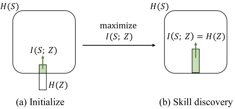
Figure 1: Information diagrams for maximizing $I(S;Z)$. (a) The information shared between the states and skills (i.e., $I(S;Z)$) is less than $H(Z)$. (b) By maximizing the variational bound, the MI objective is maximized and we have $I(S;Z)=H(Z)$.

3.1 Limitation of Previous MI Objective

In skill discovery, a skill refers to a kind of behavior that can be represented by a set of semantically meaningful trajectories labeled by a fixed latent variable $z\sim{\mathcal{Z}}$, indicating that one skill should map to a set of states. Formally, we have the following assumption.

Assumption 1.

The skill space $Z$ is smaller than the state visitation space, i.e., $H(Z)<H(S)$ with $s\sim\rho_{\pi}(s)$.

Empirically, Assumption 1 holds even with a random policy since RL tasks often have high-dimensional state space, while the skill is a discrete or continuous vector with low dimensions. In contrast, if the skill space is equal or even larger than the state space, we have many-to-one mapping from skill to state, which makes the skills indistinguishable. Meanwhile, since the skill space is often set as a discrete or uniform distribution with fixed entropy, $H(Z)$ is a constant and is irrelevant to the optimization objective of $I(S;Z)=H(Z)-H(Z|S)$.

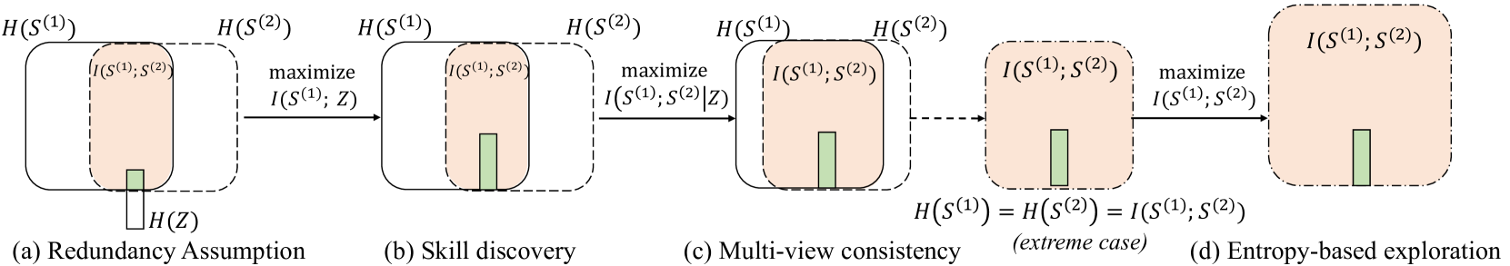
Figure 2: Information diagrams of the learning process in BeCL. (a) We show the redundancy assumption of skill between different views. (b) BeCL performs skill discovery by maximizing $I(S;Z)$ and (c) learns multi-view consistency by maximizing $I(S^{(1)};S^{(2)}|Z)$. (d) Considering the maximum empowerment and perfect multi-view consistency, our objective directly maximizes the state coverage.

We illustrate the information diagrams for maximizing $I(S;Z)$ in Figure 1. (i) As shown in Figure 1(a), since the states are generated by the skill-conditional policy and the policy is randomly initialized, the states and skills usually share a small amount of information and $I(S;Z)\geq 0$. (ii) As we learn a discriminator and train the policy to maximize the discriminability of skills, the MI term $I(S;Z)$ increases and approaches $H(Z)$. As in Figure 1(b), when the MI objective is fully optimized, the information of $I(S;Z)$ is contained in $H(Z)$. Under Assumption 1, we have

$$\max I(S;Z)=\max H(Z)-H(Z|S)=H(Z),$$ (1)

where $\min H(Z|S)=0$ due to the non-negativity of entropy, and $\max H(Z)=H(Z)$ since $H(Z)$ is fixed.

The major limitation of above optimization process is such an MI objective can hinder better state coverage and learn static skills. Specifically, the optimization objective is irrelevant to the state visitation entropy under Assumption 1 and we have $\max I(S;Z)=H(Z)$ with different $H(S)$. Considering there are two policies $\pi_{1}$ and $\pi_{2}$, where $\pi_{2}$ has better state coverage. Then the relationship between the corresponding state entropy measured by the states visited by the two policies is $H_{\rho_{\pi_{1}}}(S)<H_{\rho_{\pi_{2}}}(S)$. Nevertheless, for both policies, the maximum values of the $I(S;Z)$ objective are equal to $H(Z)$, which is irrelevant to their state entropy as shown in Eq. (1). Since there is no gradient to encourage the agent to update from $\pi_{1}$ to $\pi_{2}$, the MI objective can easily obtain its maximum, which discourages the agent from learning far-reaching skills. We remark that such a problem has also been mentioned in previous studies (Campos et al., 2020; Park et al., 2022), where they observe the agent visits marginally different states to learn distinguishable skills (e.g., with different static postures). Nevertheless, we highlight that we give an information-theoretical perspective and propose an alternative MI-objective to solve this problem.

3.2 The BeCL Objective

In this section, we introduce the proposed BeCL objective and show how our objective addresses above limitations. We consider a multi-view setting where each skill $z_{i}$ generates two trajectories $\tau^{(1)}$ and $\tau^{(2)}$ based on the skill-conditional policy. The trajectories $\tau^{(1)}$ and $\tau^{(2)}$ usually have differences since (i) the skill has limited empowerment to behaviors in the early stage of training and (ii) the transition function and policy are often stochastic. Based on $\tau^{(1)}$ and $\tau^{(2)}$, we sample two states by following

$$s^{(1)}\sim\tau^{(1)},\quad s^{(2)}\sim\tau^{(2)},$$

where $\tau^{(1)},\tau^{(2)}\sim\pi(a|s,z_{i}),\forall i$. We remark that $s^{(1)}$ and $s^{(2)}$ are generated with the same skill and denote the corresponding random variables by $S^{(1)}$ and $S^{(2)}$, respectively.

Similar to multi-view representation that assumes each view shares the same task-relevant information (Federici et al., 2020; Fan & Li, 2022), we assume that $S^{(1)}$ and $S^{(2)}$ share the same skill-relevant information since they are generated on the same skill vector $z$. Formally, we give the following mutual redundancy assumption in skill discovery.

Assumption 2 (Redundancy).

The states $S^{(1)}$ and $S^{(2)}$ are mutually redundant to the skill-relevant information, i.e., $S^{(1)}\perp\!\!\!\perp Z|S^{(2)}$ or equivalently $I(S^{(1)},Z|S^{(2)})=0$.

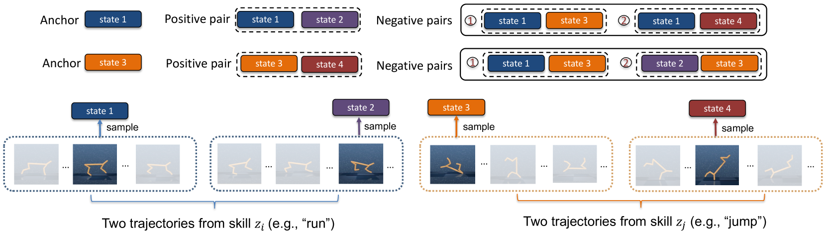
Figure 3: An illustration of the process of contrastive estimation in BeCL. We take two states of different trajectories generated by the same skill as positive samples. In addition, we find that sampling positive pairs from the same trajectory that are far from each other is also well-performed. Meanwhile, we take states of different trajectories generated by different skills as negative samples. Consider state 1 as example, we use (state 1, state 2) as positive pair, and then use (state 1, state 3) and (state 1, state 4) as negative pairs. The contrastive loss and intrinsic reward are computed in Eq. (8) and Eq. (10), respectively.

Under Assumption 2, we have

$$I(S^{(1)};Z)=I(S^{(2)};Z)=I(S^{(1)};S^{(2)};Z).$$ (2)

where the last term is multivariate MI. The proof is given in Appendix A. We remark that Assumption 2 does not indicate that the skill has good discriminability (i.e., $I(S,Z)$ is large) initially, but only assuming that the skill information shared between different views (i.e., $S^{(1)}$, $S^{(2)}$) are the same since they are generated by the same skill, as shown in Eq. (2). In most cases, the redundancy assumption holds unless the policy network does not extract any skill information. An illustration of this assumption is given in Figure 2(a).

Based on the redundancy assumption, we propose a novel MI objective for our method, as

$$I_{\rm BeCL}=I(S^{(1)};S^{(2)}).$$ (3)

To analyze the objective, we decompose $I_{\rm BeCL}$ as

$$I_{\rm BeCL}=I(S^{(1)};S^{(2)})$$ (4)

$$=I(S^{(1)};S^{(2)};Z)+I(S^{(1)};S^{(2)}|Z)$$

$$=\underbrace{\nicefrac{{1}}{{2}}\big{[}I(S^{(1)};Z)+I(S^{(2)};Z)\big{]}}_{(i)~{}\rm skill\>\>discovery}\>+\!\!\!\underbrace{I(S^{(1)};S^{(2)}|Z)}_{(ii)~{}\rm multi-view\>\>consistency},$$

where the last equation follows Eq. (2). We analyze the optimization process of $I_{\rm BeCL}$ as follows.

(1) Skill discovery. Maximizing term $(i)$ in Eq. (4) is equivalent to maximizing $I(S;Z)$ in previous skill discovery methods, where $s\sim S$ can be sampled from $S^{(1)}$ or $S^{(2)}$. As a result, our objective serves as an upper bound of $I(S;Z)$ in previous MI objective (Gregor et al., 2016). As shown in Figure 2(b), this objective expands the information shared between $Z$ and $(S^{(1)},S^{(2)})$. In practice, since $H(Z)$ is much smaller than $H(S)$, this term is relatively easy to optimize to achieve its maximum value (i.e., $H(Z)$).

(2) Multi-view consistency. The empowerment of skill to the resulting states is maximized when term $(i)$ in Eq. (4) achieve $H(Z)$. Then the differences between two views (i.e., $S^{(1)}$ and $S^{(2)}$) come from the randomness of the environment and the policy. As shown in Figure 2(c), through maximizing the second term in Eq. (4) (i.e., $I(S^{(1)},S^{(2)}|Z)$), the skills will learn to make the explored policy less sensitive to environmental randomness and also drive the policy becomes deterministic, which leads to better multi-view consistency of states based on the same skill. We remark that such an effect is different from previous methods that maximize the policy entropy to keep the policy stochastic (Eysenbach et al., 2019). Nevertheless, we remark that a deterministic skill-conditional policy can also have a well state coverage by generating far-reaching trajectories. The multi-view consistency makes trajectories sampled with the same skill explore the nearly areas and have better alignment.

(3) Entropy-based Exploration. In Figure 2(c), we show an extreme case that $S^{(1)}$ and $S^{(2)}$ are completely consistent by optimizing the multi-view consistency in our objective. In this case, we have the relationship $I(S^{(1)};S^{(2)})=H(S^{(1)})=H(S^{(2)})$ holds, thus maximizing our objective directly maximizes the entropy of explored states. We highlight that such a property addresses the limitation of the previous MI objective. As illustrated in Figure 2(d), the state coverage increases as we encourage the policy to increase the state visitation entropy. Although such a complete consistency case is unachievable in practice, we will show that BeCL indeed maximizes the state entropy through contrastive estimation of our MI objective in the following.

3.3 Behavior Contrastive Learning

To estimate the MI objective in high-dimensional state space, a tractable variational estimator based on neural networks is required (Poole et al., 2019). In BeCL, we adopt contrastive learning (Oord et al., 2018) to approximate the objective, as

$$L_{\rm BeCL1} ={\mathbb{E}}_{z_{i},\{z_{j}\}\sim p(z),(s_{i}^{(1)},s_{i}^{(2)})\sim p(\cdot|z_{i})}{\mathbb{E}}_{s_{j}\sim p(\cdot|z_{j}),\forall z_{j}\neq z_{i}}$$ (5)

$$\left[-\log\>\>\frac{h(s^{(1)}_{i},s^{(2)}_{i})}{\sum_{s_{j}\in S^{-}\bigcup s^{(2)}_{i}}h(s^{(1)}_{i},s_{j})}\right],$$

where $z_{i}$ and $z_{j}$ are skills sampled from a discrete skill distribution $p(z)$. A positive pair $[s^{(1)}_{i}$, $s^{(2)}_{i}]$ contains two states sampled from trajectories based on the same skill-conditional policy $\pi(a|s,z_{i})$. In contrast, a negative pair $[s^{(1)}_{i},s_{j}]$ is constructed by sampling $s_{i}$ and $s_{j}$ based on different skills $z_{i}$ and $z_{j}$. In Eq. (5), we use a negative sample set $S^{-}$ to represent the states sampled from $\{z_{j}\}$, where $z_{j}\neq z_{i}$. Since $s_{i}$ and $s_{j}$ are sampled independently by different skills, we expect their similarity to be much smaller than that of positive pairs. The score function is an exponential similarity measurement between states, as

$$h(s_{i},s_{j})=\exp\big{(}f_{\phi}(s_{i})^{\top}f_{\phi}(s_{j})\big{)},$$ (6)

where $f_{\phi}(\cdot)$ is an encoder network with normalization to make $\|f_{\phi}(\cdot)\|=1$. The function $h(\cdot,\cdot)$ aims to assign high scores for positive pairs and low scores for negative pairs.

An illustration of the contrastive learning process is given in Figure 3. We sample $m$ skills $\{z_{i}\}_{i\in[m]}$ and generate two trajectories for each skill when interacting with the environment. Based on the trajectories $\{\tau^{(1)}_{i},\tau^{(2)}_{i}\}_{i\in[m]}$, we sample a state from each trajectory, which gives a positive pair as $\{s^{(1)}_{i},s^{(2)}_{i}\}_{i\in[m]}$. Then, we construct the negative pairs by sampling states come from trajectories based on different skills. For each anchor state, we use the corresponding positive state and $2(m-1)$ negative states to calculate the contrastive loss.

Theorem 1.

The relationship between our MI objective in Eq. (2) and the contrastive loss defined in Eq. (5) is

$$I_{\rm BeCL}=I(S^{(1)};S^{(2)})\geq\log N-L_{\rm BeCL1},$$ (7)

where $N=2m-1$ and $m$ is the number of sampled skills.

The proof is given in Appendix A. Since $N$ is a constant, minimizing the contrastive loss will maximize our MI objective $I(S^{(1)};S^{(2)})$. As discussed in Figure 2, maximizing $I(S^{(1)};S^{(2)})$ can perform skill discovery, improve the multi-view consistency, and improve the state coverage.

Comparing to other RL algorithms that use data augmentation (Laskin et al., 2020), dynamics consistency (Mazoure et al., 2020), or temporal information (Eysenbach et al., 2022) for contrastive learning, we provide a novel way by using skills to construct positive and negative pairs, which extracts skill-relevant information for unsupervised RL.

3.4 Qualitative Analysis

In practice, we follow SimCLR (Chen et al., 2020) by using a small temperature $\kappa<1$ in our contrastive objective to control the strength of penalties. Specifically, we define

$$L_{\rm BeCL2}={\mathbb{E}}_{\>i,j\in[m],s^{(1)}_{i},s^{(2)}_{i},s_{j}}$$ (8)

$$=\left[-\log\frac{\exp\big{(}f(s^{(1)}_{i})^{\top}f(s^{(2)}_{i})/\kappa\big{)}}{\sum_{s_{j}\in S^{-}\bigcup s_{i}^{(2)}}\exp\big{(}f(s_{j})^{\top}f(s^{(1)}_{i})/\kappa\big{)}}\right].$$

There are two effects in optimizing Eq. (8) in skill discovery. (i) The positive pairs in the numerator become similar in the feature space, achieving better multi-view alignment for trajectories based on the same skill. For implementation, $s_{i}$ or $s_{j}$ in Eq. (8) can also be replaced by other information (e.g., sub-trajectory) to capture the long-term consistency. (ii) The negative samples in the denominator have repulsive force to each other, which will push the states in one skill away from states in other skills. Finally, the states of different skills will roughly be uniformly distributed in the state space, which helps the agent improve the state coverage.

Formally, since the state features lie on a hypersphere, i.e., $\{f(s)\in\mathbb{R}^{d}:\|f(s)\|=1\}$, we adopt the von Mises-Fisher (vMF) distribution as a spherical density function to perform kernel density estimation (KDE) (Di Marzio et al., 2019; Wang & Isola, 2020). The following theorem establishes the relationship between the contrastive objective $L_{\rm BeCL2}$ and the state entropy estimation (Beirlant et al., 1997).

Theorem 2.

With sufficient negative samples, minimizing $L_{\rm BeCL2}$ can maximize the state entropy, as

$$\!\!\lim_{N\rightarrow\infty}\!L_{\rm BeCL2}\!=\!-\frac{1}{\kappa}{\mathbb{E}}_{s_{i}}[f(s^{(1)}_{i})^{\top}f(s^{(2)}_{i})]-\hat{H}\big{(}f(s)\big{)}+\log C,$$ (9)

where $\hat{H}(\cdot)$ is a resubstitution entropy estimator through the von Mises-Fisher (vMF) kernel density estimation, and $\log C$ is a normalization constant.

A detailed proof is given in Appendix A. In Theorem 2, the vMF kernel has a concentration parameter $\kappa^{-1}$, which controls how peaky of the distribution is around its referenced feature in entropy estimation. In practice, we set $\kappa=0.5$ to obtain a reasonable result. According to Theorem 2, the first term of Eq. (9) is related to skill discovery methods (Eysenbach et al., 2019; Liu & Abbeel, 2021b) by improving the multi-view alignment to increase the empowerment of skills. The second term is similar to data-based unsupervised RL methods (Liu & Abbeel, 2021a; Laskin et al., 2022) as they explicitly measure the state entropy through a particle entropy estimator, while we maximize the state entropy implicitly via contrastive learning.

For unsupervised RL training, we set the intrinsic reward to

$$r(s_{i}^{(1)})\!:=\!{\mathbb{E}}_{s_{i}^{(2)},s_{j}}\!\!\left[\frac{\exp\big{(}f(s^{(1)}_{i})^{\top}f(s^{(2)}_{i})/\kappa\big{)}}{\sum_{s_{j}\sim S^{-}\bigcup s_{i}^{(2)}}\exp\big{(}f(s_{j})^{\top}f(s^{(1)}_{i})/\kappa\big{)}}\right],$$ (10)

where we estimate the reward by sampling $s_{i}^{(2)}$ and $S^{-}$ from a training batch that contains $2m$ trajectories. Then we use the intrinsic reward for policy training. The algorithmic description of our method is given in Appendix C.3.

4 Related Works

Unsupervised Skill Discovery

Unsupervised skill discovery allows agents to learn discriminable behavior by maximizing the MI between states and skills (Gregor et al., 2016; Florensa et al., 2017; Eysenbach et al., 2019; Sharma et al., 2020; Baumli et al., 2021). However, many works (Laskin et al., 2021, 2022; Strouse et al., 2022) have shown that skill learning through variational MI maximization provides a poor coverage of state space, which may affect its applicability to downstream tasks with complex environments. Some methods consider restricting the observation space of skill learning to x-y Cartesian coordinates to increase in traveled distances (or variations) in the coordinate space (called the x-y prior) (Park et al., 2022; Zhao et al., 2021). However, these methods introduce strong assumptions in learning skills and are mainly narrow in navigation tasks and a few other tasks with coordinate information. In addition, other methods also propose auxiliary exploration mechanisms or training techniques (Strouse et al., 2022; Bagaria et al., 2021; Barreto et al., 2019; Campos et al., 2020; Jiang et al., 2022) to tackle the problem of state coverage. In contrast, our approach learns diverse skills without limiting the observation space, and also implicitly increases the state entropy to encourages exploration without auxiliary losses.

Unsupervised RL

Unsupervised RL algorithms focus on training a general policy for fast adaptation to various downstream tasks. Unsupervised RL mainly contains two stages: pretrain and finetune. The core of unsupervised RL is to design an intrinsic reward in the pretrain stage. URLB (Laskin et al., 2021) broadly divides existing algorithms into three categories. The data-based approaches encourage the agent to collect novel states in pretraining through maximization of state entropy (Liu & Abbeel, 2021a; Yarats et al., 2021; Laskin et al., 2022); the knowledge-based approaches enable agents to learn behavior based on the output of some model prediction (i.e. curiosity, surprise, uncertainty, etc.) (Pathak et al., 2017, 2019; Burda et al., 2019; Hao et al., 2023; Bai et al., 2021c, a); and the competence-based approaches maximize the agent empowerment over environment from the perspective of information theory, which means the agent is trained to discover what can be done in an environment while learning how to achieve it (Lee et al., 2019; Eysenbach et al., 2019; Liu & Abbeel, 2021b). Our method can be regarded as a novel competence-based approach as we can make each skill learn potential behavior that is useful for downstream tasks and also improve the state coverage.

Contrastive Learning

Contrastive learning is a representation learning framework in deep learning (He et al., 2020; Caron et al., 2020; Grill et al., 2020; Radford et al., 2021). The main idea is to define positive and negative pairs to learn useful representations. Contrastive learning has also been used in RL as auxiliary tasks to improve the sample efficiency. Positive and negative pairs in RL can be constructed following state enhancement (Laskin et al., 2020), temporal consistency (Sermanet et al., 2018), dynamic-relevant transition (Mazoure et al., 2020; Bai et al., 2021b; Qiu et al., 2022), return estimation (Liu et al., 2021), or goal information (Eysenbach et al., 2022). Unlike these methods, we use skills to divide the positive and negative pairs. Recently proposed CIC (Laskin et al., 2022) performs contrastive learning to approximate $I(S;Z)$ and uses the learned representation for entropy estimation. In contrast, we propose a different contrastive objective through a multi-view perspective and use the objective as an intrinsic reward. Our method is related to the alignment and uniformity properties of contrastive learning mentioned in Wang & Isola (2020). Our contrastive objective also learns uniformly distributed state representations to improve the state coverage.

5 Experiments

In this section, we first provide qualitative analysis for the behaviors of different skills learned in BeCL and other competence-based methods in a 2D continuous maze and challenging continuous control tasks from the DeepMind Control Suite (DMC) (Tassa et al., 2018). We then compare the adaptation efficiency of the learned skills in downstream tasks of URLB (Laskin et al., 2021), where previous competence-based methods shown to produce relatively weak performance. We finally conduct several ablation studies on skill finetuning, skill dimensions, and temperature.

5.1 Continuous 2D Maze

We start from a continuous 2D maze to illustrate the skills learned in BeCL. We adopt the environment of Campos et al. (2020), where the agent observes its current position (${\mathcal{S}}\in{\mathbb{R}}^{2}$) and takes an action (${\mathcal{A}}\in{\mathbb{R}}^{2}$) to control its velocity and direction. The agent will be blocked if it collides with the wall. We make comparisons with three typical skill optimization objectives from DIAYN (Eysenbach et al., 2019), DADS (Sharma et al., 2020), and CIC (Laskin et al., 2022). Specifically, DIAYN maximizes the reverse form of MI as $I(S;Z)=H(Z)-H(Z|S)$, DADS maximizes the forward form of MI as $I(S;Z)=H(S)-H(S|Z)$, and CIC is a data-based method that maximizes the state entropy $H(S)$ with a particle estimator. For a fair comparison, all methods sample skills from a 10-dimensional discrete distribution and follow the same training procedure. The differences between methods are the formulation of intrinsic rewards and representations.

Question 1.

Can BeCL balance skill empowerment and state coverage?

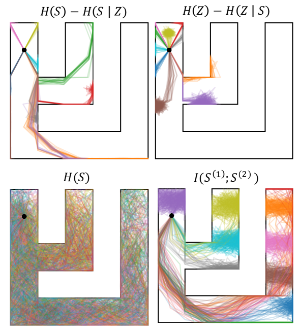
Figure 4: A illustration of different skill discovery objectives. The initial state is denoted by a black dot and the color of the trajectories denote different skill upon which it was conditioned. We generate 20 trajectories for each skill. Top: the reverse (Eysenbach et al., 2019) and forward (Sharma et al., 2020) forms for optimizing $I(S;Z)$ can discover discriminable skills but fail to reach the right side of the maze. Bottom left: Maximizing the state entropy allows skills to cover the entire space of maze, while different skills cannot be distinguished from each other (Laskin et al., 2022). Bottom right: BeCL learns skills that are distributed in different areas with well alignment in the same skill, indicating that BeCL can balance state coverage and empowerment in skill discovery.

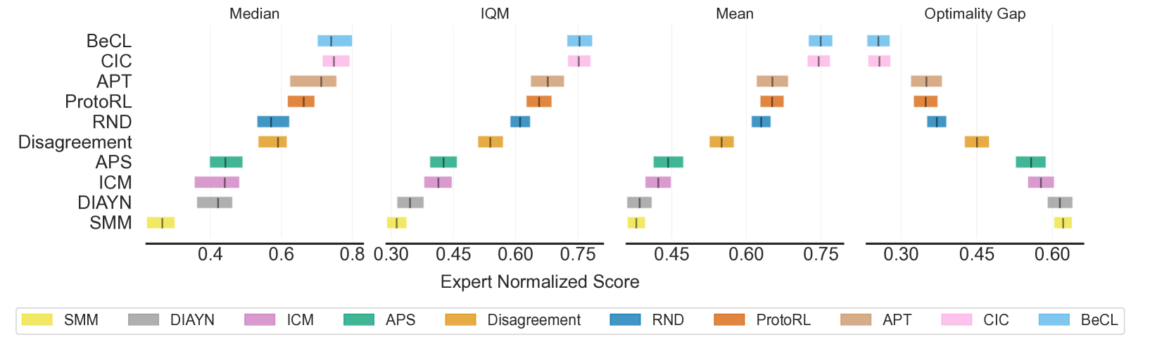
Figure 5: The aggregate statistics indicate the adaptation performance of different unsupervised RL methods in 12 downstream tasks. We run all baselines for 10 seeds and report the aggregated normalized score (Agarwal et al., 2021) after 100K steps of finetune. BeCL obtains the highest Interquratile Mean (IQM) score of 75.38% and the lowest Optimality Gap (OG) score of 25.44%.

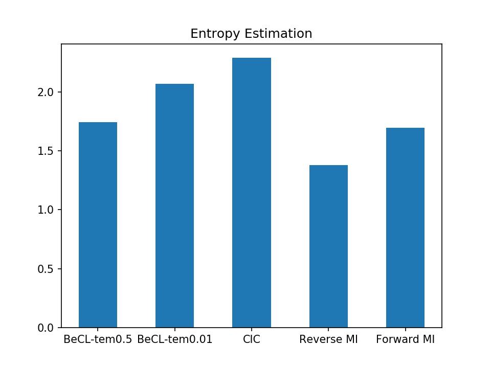
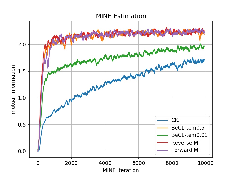
Figure 8: We compare the mutual information (MI) estimation and the entropy estimation in maze. Specifically, we generate several trajectories for each learned skill and perform MI estimation using MINE (Belghazi et al., 2018) and entropy estimation using the particle-based entropy estimator (Liu & Abbeel, 2021a). The result shows that CIC obtains much lower MI than other skill discovery methods but obtains the largest state entropy. BeCL can balance state coverage and empowerment with different temperature parameters, which leads to diverse skills and also better state coverage than previous MI-based algorithms.

We visualize the trajectories generated by different skills in maze and compare BeCL to other skill discovery methods in Figure 4. We find DIAYN and DADS produce discriminable skills while the trajectories are not far-reaching. In contrast, CIC can produce skills with the best state coverage, while the trajectories of different skills are mixed and lack of diversity. Since CIC maximizes the state entropy via a k-nearest-neighbor estimator and maps states from the same skill to similar representations, the closest $k$-th neighbors can also include states conditioned on the same skill. Maximizing the state entropy will push these states away from each other and leads to an increase in $H(S|Z)$. In contrast, BeCL maps the states from the same skill into similar features to encourage better empowerment; meanwhile, it also pushes states in one skill away from states in other skills to obtain diverse skills and better state coverage. We provide further numerical analysis of mutual information and entropy estimation between the methods in the maze, as shown in Figure 8 in Appendix B.

5.2 URLB Environments

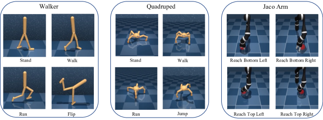
Figure 9: Introduction of domains and their downstream tasks in URLB (Laskin et al., 2021). There are four different domains and each domain has four different downstream tasks. The environment is based on DMC (Tassa et al., 2018). The episode lengths for the Walker and Quadruped domains are set to 1000, and the episode length for the Joco domain is set to 250, which results in the maximum episodic reward for the Walker and Quadruped domains being 1000, and for Jaco Arm being 250.

We evaluate BeCL in DMC tasks from URLB benchmark (Laskin et al., 2021), which needs to discover more complicated skills to achieve the desired behavior. URLB consists of three different domains, including Walker, Quadruped, and Jaco Arm. Each domain contains four downstream tasks. Specifically, Walker is a biped constrained to a 2D vertical plane (i.e. ${\mathcal{S}}\in{\mathbb{R}}^{24},{\mathcal{A}}\in{\mathbb{R}}^{6}$), which has four different locomotion tasks including (Walker, Stand), (Walker, Run), (Walker, Flip) and (Walker, Walk); Quadruped is a quadruped with four downstream tasks including (Quadruped, Stand), (Quadruped, Run), (Quadruped, Jump) and (Quadruped, Walk), while it is more challenging due to the higher-dimensional states and actions spaces (i.e. ${\mathcal{S}}\in{\mathbb{R}}^{78},{\mathcal{A}}\in{\mathbb{R}}^{16}$) and complex dynamics; Jaco Arm is a 6-DoF robotic arm with a three-finger gripper (i.e. ${\mathcal{S}}\in{\mathbb{R}}^{55},{\mathcal{A}}\in{\mathbb{R}}^{9}$) and its downstream tasks aim to reach and manipulate a movable diamond with different positions. We illustrate more details about the tasks in Figure 9 of Appendix C

Question 2.

What skills do BeCL learn in DMC?

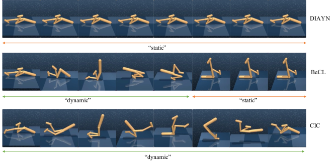
Figure 10: Qualitative visualization for the behavior of different competence-based algorithms on Walker domain from URLB. From left to right, the figures show the snapshots of behaviors from the three algorithms within an episode. We find that DIAYN polices produce constantly static and non-trivial poses, while CIC policies can produce dynamic and trivial behaviors, which is consistent with the observations of previous work (Laskin et al., 2022, 2021). In contrast, BeCL combines dynamic and static behaviors during an episode, which can also be use for good adaptation in downstream tasks.

We provide a qualitative analysis of the behavior of skills in more complex control tasks. We compare BeCL to other competence-based algorithms including CIC and DIAYN in Walker domain. As shown in Figure 10 in Appendix C.4, with the same pretraining steps, BeCL produces dynamic and non-trivial behavior during a finite episode. In contrast, solely maximizing state entropy like CIC leads to trivial and dynamic behavior since it encourages the agent to collect unusual states, such as visiting ‘handstands’ state by constantly trying to wiggle the agent’s body for larger reward. In addition, DIAYN learns static ‘posing’ skills since the static skills can also optimize the MI objective $I(S;Z)$, as we discuss in Section 3.1.

Question 3.

How does the adaptation efficiency of BeCL compared to other unsupervised RL algorithms?

Baselines.

We compare BeCL with other baselines in the URLB benchmark, including knowledge-based, data-based, and competence-based algorithms. Knowledge-based methods include ICM (Pathak et al., 2017), Disagreement (Pathak et al., 2019), and RND (Burda et al., 2019); data-based methods include APT (Liu & Abbeel, 2021a), ProtoRL (Yarats et al., 2021), and CIC (Laskin et al., 2022); and competence-based methods include SMM (Lee et al., 2019), DIAYN (Eysenbach et al., 2019), and APS (Liu & Abbeel, 2021b). The main difference between baselines are the design of intrinsic reward and representation. We summarize the implementation details of the baselines in Appendix C.2. We follow the hyper-parameters and the implementation recommended by URLB and CIC.

Evaluation.

To perform a fair comparison, we follow standard pretraining and finetuning procedures as suggested in URLB (Laskin et al., 2021). We pretrain each algorithm for 2M steps with only intrinsic rewards for each domain, and then finetune the policy for 100K steps in different downstream tasks with extrinsic reward. We use DDPG (Lillicrap et al., 2016) as the basic RL algorithm and train each method for 10 seeds, resulting in 1200 runs in total (i.e., $10$ algorithms $\times$ $10$ seeds $\times$ $3$ domains $\times$ $4$ tasks).

Following reliable (Agarwal et al., 2021), we adopt interquartile mean (IQM) and optimality gap (OG) metrics aggregated with stratified bootstrap sampling as our main evaluation metrics across all runs. IQM discards the bottom and top 25% of the runs and calculates the mean score of the remaining 50% runs. OG evaluates the amount by which the algorithm fails to meet a minimum score of desired target. The expert score is obtained by running DDPG with 2M steps in the corresponding tasks and we adopt the expert scores from Laskin et al. (2022). We normalize each score with the expert score and the statistical results are shown in Figure 5. In the IQM metric, BeCL achieves competitive performance with CIC (75.38% and 75.18%, respectively) and outperforms the next best skill discovery algorithm (i.e., APS) by 38.2%. In OG metric, BeCL achieves the closest performance to expert performance (around 25.44%) and the CIC score achieves approximately 25.75%.

5.3 Ablation Study

Question 4.

Whether different skills have different adaptation efficiency on downstream tasks?

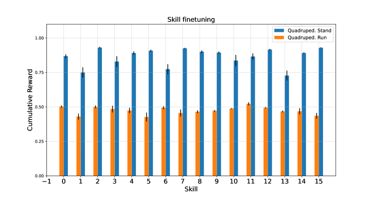
Figure 11: The adaptation efficiency of difference skills in the finetuning stage. The skill is a one-hot vector sampled from a 16-dimensional discrete distribution in the pretraining stage. Then we sample each skill for finetuning in (Quadruped, Run) and (Quadruped, Stand) tasks. We find that some skills do not always obtain a well generalization performance in downstream tasks (e.g. skill 1,6,13 in stand task). In BeCL, we uniformly choosing skill in the finetuning stage to evaluate the average adaptation performance among skills, although it would be better to choosing the best skills through a grid search like CIC (Laskin et al., 2022). We believe more matching meta-controller or other effective finetuning methods should be considered in future works.

We evaluate the adaptation efficiency of the learned skills in pretraining the Quadruped agent. We compare the normalized reward after finetuning by initializing the policy with different skills vector. We show the downstream performance in (Quadruped, stand) and (Quadruped, run) tasks in Figure 11 of Appendix C. We find that the performance of different skills does not always revolve around statistical averages and some skills have relatively weak adaptation ability, which indicates that a skill-chosen process would be desired before finetuning. For example, CIC (Laskin et al., 2022) chooses skills with grid sweep in the first 4K finetuning steps. In contrast, BeCL randomly samples skills in the finetuning stage to report the average performance of skills, which provides a more comprehensive evaluation of the learned skills.

Question 5.

How does the skill dimensions affect unsupervised skill discovery?

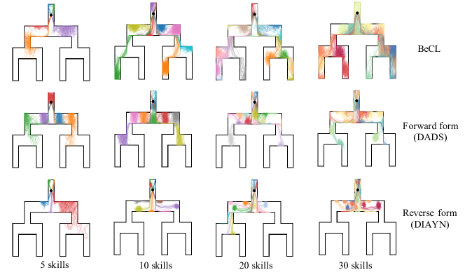
Figure 7: A illustration of the impact of different numbers of skills in tree-like Mazes. All methods are trained for 2500 episodes, and each episode allows 50 interactions with environment. As the skill dimension increases, skills of DIAYN and DADS still optimize MI in a narrow area of the maze and cannot reach deeper position. In contrast, BeCL skills gradually cover the whole state space by applying more skills to explore the maze and more negative samples to provide a better state-entropy estimator.

We explore the impact of the skill dimensions with a discrete skill space. We train DIAYN (Eysenbach et al., 2019), DADS (Sharma et al., 2020) and BeCL with different numbers of skill in a tree-like maze. As shown in Figure 7 of Appendix B, with the skill dimension increases, DIAYN and DADS still optimize MI in a narrow area of the maze and cannot go far away. In contrast, BeCL skills gradually cover the entire maze when the skill dimension increases, which coincides to Theorem 2 that using more skills increases the number of negative samples and provides a better entropy estimator. We further study the impact of the skill dimension on adaptation efficiency in DMC, as shown in Figure 12 of Appendix C. The results show that increasing the skill dimension can benefit the adaptation performance in hard downstream tasks (e.g. (Walker, Run) and (Walker, Flip)), while it cannot improve the performance in relatively easy tasks approaching expert scores (e.g. (Walker, Stand)).

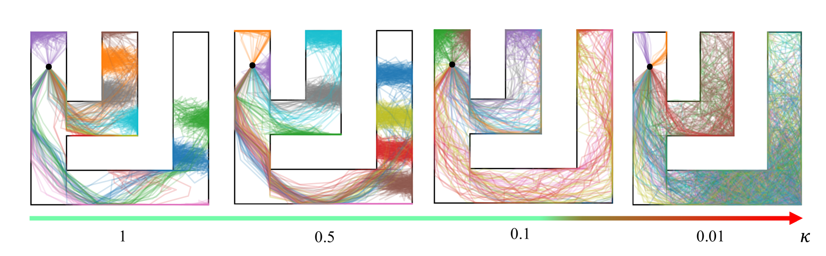
Figure 6: The impact of temperature $\kappa$ in the behavior of BeCL. Lower temperatures encourage more skills to cover the right side of the maze (e.g. temperature from 1 to 0.5). But as the temperature dropped further (e.g. temperature from 0.1 to 0.01), some skills tend to produce more dispersed trajectories. This makes some skills indistinguishable from each other in a confined maze.

Question 6.

How does the temperature $\kappa$ in the contrastive objective affect empowerment and state coverage?

To analyze the effect of temperature $\kappa$ on the behavior of BeCL skills, we evaluate several values of $\kappa$ in the maze task. The result is shown in Figure 6. We find that using a smaller temperature value encourages the skills to explore the entire maze space (i.e., decreases from 1 to 0.5). However, as the temperature decreases further (i.e., decreases from 0.1 to 0.01), trajectories from different skills tend to be more uniformly distributed, which somewhat weakens the discriminability of skills. We remark that such a scenario resembles previous analysis of temperature (Wang & Liu, 2021; Wang & Isola, 2020), where $\kappa$ is considered to balance the uniformity-tolerance dilemma in unsupervised contrastive learning. Specifically, we hope that the skills can be distributed uniformly to be globally separated; meanwhile, we hope that the trajectories are locally clustered and are more tolerant to the states generated with the same skill. A suitable $\kappa$ may avoid the gathering of different skills in local areas, which helps to explore different regions and improves the state coverage. Meanwhile, too small $\kappa$ can be harmful to the alignment of positive samples, which weakens the empowerment of skills.

6 Conclusion

We propose BeCL with a novel MI objective for unsupervised skill discovery from a multi-view perspective. Theoretically, BeCL discovers skills and maximizes the state coverage simultaneously, which makes BeCL produce diverse behaviors in various skills. Empirical results show that BeCL learns diverse and far-reaching skills in mazes and performs well in downstream tasks of URLB. In the future, we will improve BeCL by selecting hard negative samples to obtain a tighter MI bound, and developing a meta-controller for better skill selection in the finetuning stage.

Appendix A Theoretical Proof

A.1 Proof of the MI Decomposition

Under Assumption 2, we recall that Eq. (2) is

$$I(S^{(1)};Z)=I(S^{(2)};Z)=I(S^{(1)};S^{(2)};Z).$$

Proof.

For random variables $X$, $Y$ and $Z$, the chain rule for multivariate MI is

$$I(X;Y;Z)=I(Y;Z)-I(Y;Z|X).$$ (11)

Thus, for $S^{(1)}$, $S^{(2)}$, and $Z$, we have the similar relationship as

$$I(S^{(1)};Z)=I(S^{(1)};S^{(2)};Z)+I(S^{(1)};Z|S^{(2)}).$$ (12)

According to the redundancy assumption in Assumption 2, we have

$$I(S^{(1)};Z\>\big{|}\>S^{(2)})=0,$$ (13)

and then we have

$$I(S^{(1)};Z)=I(S^{(1)};S^{(2)};Z).$$ (14)

Following a similar proof, we have

$$I(S^{(2)};Z)=I(S^{(1)};S^{(2)};Z),$$ (15)

which conclude our proof. ∎

A.2 Proof of Theorem 1

Theorem (Theorem 1 restate).

The relationship between our MI objective in Eq. (2) and the contrastive loss defined in Eq. (5) is

$$I_{\rm BeCL}=I(S^{(1)};S^{(2)})\geq\log N-L_{\rm BeCL1},$$ (16)

where $N=2m-1$ and $m$ is the number of sampled skills.

Proof.

We rewrite $L_{\rm BeCL1}$ defined in Eq. (5) with $m$ discrete skills as

$$L_{\rm BeCL1}={\mathbb{E}}_{i\in[m],s_{i}^{(1)},s_{i}^{(2)},s_{j}}\left[-\log\>\>\frac{h(s^{(1)}_{i},s^{(2)}_{i})}{\sum_{s_{j}\in S^{-}\bigcup s^{(2)}_{i}}h(s^{(1)}_{i},s_{j})}\right],$$

Following the definition of MI, we have

$$I(S^{(1)};S^{(2)})-\log N ={\mathbb{E}}_{i\in[m],s^{(1)}_{i},s^{(2)}_{i}}\left[\log\frac{p(s^{(1)}_{i}s^{(2)}_{i})}{p(s^{(1)}_{i})p(s^{(2)}_{i})}\right]-\log{N}$$ (17)

$$={\mathbb{E}}_{i\in[m],s^{(1)}_{i},s^{(2)}_{i}}\left[\log\frac{p(s^{(1)}_{i}|s^{(2)}_{i})}{p(s^{(1)}_{i})}\right]-\log{N}$$

$$={\mathbb{E}}_{i\in[m],s^{(1)}_{i},s^{(2)}_{i}}\left[\log\frac{1}{\frac{p(s^{(1)}_{i})}{p(s^{(1)}_{i}|s^{(2)}_{i})}N}\right]$$

$$={\mathbb{E}}_{i\in[m],s^{(1)}_{i},s^{(2)}_{i}}\left[\log\frac{1}{\frac{p(s^{(1)}_{i})}{p(s^{(1)}_{i}|s^{(2)}_{i})}+\frac{p(s^{(1)}_{i})}{p(s^{(1)}_{i}|s^{(2)}_{i})}(N-1)}\right]$$

Under Assumption 2, since $S^{(1)}$ and $S^{(2)}$ share the same information about the skill, we have $p(s^{(1)}|s^{(2)})\geq p(s^{(1)})$. Then

$$I(S^{(1)};S^{(2)})-\log N \geq{\mathbb{E}}_{i\in[m],s^{(1)}_{i},s^{(2)}_{i}}\left[\log\frac{1}{1+\frac{p(s^{(1)}_{i})}{p(s^{(1)}_{i}|s^{(2)}_{i})}(N-1)}\right]$$ (18)

$$={\mathbb{E}}_{i\in[m],s^{(1)}_{i},s^{(2)}_{i}}\left[-\log\left(1+\frac{p(s^{(1)}_{i})}{p(s^{(1)}_{i}|s^{(2)}_{i})}(N-1)\right)\right].$$ (19)

Considering we sample $s_{j}\in S^{-}$ that is independent to $s^{(1)}_{i}$ (i.e., $i\neq j$), we have $p(s^{(1)}_{i}|s_{j})=p(s^{(1)}_{i})$. Formally, we have

$${\mathbb{E}}_{j\in[m]\setminus\{i\},s_{j}\in S^{-}}\left[\frac{p(s^{(1)}_{i}|s_{j})}{p(s^{(1)}_{i})}\right]=1,$$ (20)

where $S^{-}$ contains $N-1$ negative examples. Plugging (20) into (19), we have

$$I(S^{(1)};S^{(2)})-\log N \geq{\mathbb{E}}_{i\in[m],s^{(1)}_{i},s^{(2)}_{i}}\left[-\log\left(1+\frac{p(s^{(1)}_{i})}{p(s^{(1)}_{i}|s^{(2)}_{i})}(N-1)\right)\right]$$ (21)

$$={\mathbb{E}}_{i\in[m],s^{(1)}_{i},s^{(2)}_{i}}\left[-\log\left(1+\frac{p(s^{(1)}_{i})}{p(s^{(1)}_{i}|s^{(2)}_{i})}(N-1){\mathbb{E}}_{S^{-}}\left[\frac{p(s^{(1)}_{i}|s_{j})}{p(s^{(1)}_{i})}\right]\right)\right]$$

$$={\mathbb{E}}_{i\in[m],s^{(1)}_{i},s^{(2)}_{i},s_{j}}\left[-\log\left(1+\frac{p(s^{(1)}_{i})}{p(s^{(1)}_{i}|s^{(2)}_{i})}\sum_{s_{j}\in S^{-}}\frac{p(s^{(1)}_{i}|s_{j})}{p(s^{(1)}_{i})}\right)\right]$$

$$={\mathbb{E}}_{i\in[m],s^{(1)}_{i},s^{(2)}_{i},s_{j}}\left[-\log\left(\frac{p(s^{(1)}_{i}|s^{(2)}_{i})+p(s^{(1)}_{i})\sum_{s_{j}\in S^{-}}\frac{p(s^{(1)}_{i}|s_{j})}{p(s^{(1)}_{i})}}{p(s^{(1)}_{i}|s^{(2)}_{i})}\right)\right]$$

$$={\mathbb{E}}_{i\in[m],s^{(1)}_{i},s^{(2)}_{i},s_{j}}\left[\log\left(\frac{\frac{p(s^{(1)}_{i}|s^{(2)}_{i})}{p(s^{(1)}_{i})}}{\frac{p(s^{(1)}_{i}|s^{(2)}_{i})}{p(s^{(1)}_{i})}+\sum_{s_{j}\in S^{-}}\frac{p(s^{(1)}_{i}|s_{j})}{p(s^{(1)}_{i})}}\right)\right]$$

$$={\mathbb{E}}_{i\in[m],s^{(1)}_{i},s^{(2)}_{i},s_{j}}\left[\log\left(\frac{h(s^{(1)}_{i},s^{(2)}_{i})}{h(s^{(1)}_{i},s^{(2)}_{i})+\sum_{s_{j}\sim S^{-}}h(s^{(1)}_{i},s_{j})}\right)\right],$$

where $h(x_{1},x_{2})=p(x_{1}|x_{2})/p(x_{1})$ is the score function that preserves the mutual information between $x_{1}$ and $x_{2}$. In practice, we use a neural network to represent the score function.

∎

A.3 Proof of Theorem 2

Theorem (Restate of Theorem 2).

With sufficient negative samples, minimizing $L_{\rm BeCL2}$ can maximize the state entropy, as

$$\!\!\lim_{N\rightarrow\infty}\!L_{\rm BeCL2}\!=\!-\frac{1}{\kappa}{\mathbb{E}}_{s_{i}}[f(s^{(1)}_{i})^{\top}f(s^{(2)}_{i})]-\hat{H}\big{(}f(s)\big{)}+\log C,$$ (22)

where $\hat{H}(\cdot)$ is a resubstitution entropy estimator through the von Mises-Fisher (vMF) kernel density estimation, and $\log C$ is a normalization constant.

Proof.

We rewrite the definition of our contrastive estimator as

$$L_{\rm BeCL2} ={\mathbb{E}}_{s_{i},s_{j}}\left[-\log\frac{\exp\big{(}f(s^{(1)}_{i})^{\top}f(s^{(2)}_{i})/\kappa\big{)}}{\exp\big{(}f(s^{(1)}_{i})^{\top}f(s^{(2)}_{i})/\kappa\big{)}+\sum_{s_{j}\in S^{-}}\exp\big{(}f(s_{j})^{\top}f(s^{(1)}_{i})/\kappa\big{)}}\right]$$ (23)

$$={\mathbb{E}}_{s_{i}}\left[-\frac{1}{\kappa}\big{(}f(s^{(1)}_{i})^{\top}f(s^{(2)}_{i})\right]+{\mathbb{E}}_{s_{i},s_{j}}\left[\log\left(\exp\big{(}f(s^{(1)}_{i})^{\top}f(s^{(2)}_{i})/\kappa\big{)}+\sum_{s_{j}\in S^{-}}\exp\big{(}f(s_{j})^{\top}f(s^{(1)}_{i})/\kappa\big{)}\right)\right]$$

In the following, we denote $M=N-1$ as the number of negative samples when using $s^{(1)}$ as the anchor state. Then we have

$$\lim_{M\rightarrow\infty}L_{\rm BeCL2}-\log M$$ (24)

$$={\mathbb{E}}_{s_{i}}\left[-\frac{1}{\kappa}\big{(}f(s^{(1)}_{i})^{\top}f(s^{(2)}_{i})\right]+{\mathbb{E}}_{s_{i}}\lim_{M\rightarrow\infty}\left[\log\left(\frac{1}{M}\exp\big{(}f(s^{(1)}_{i})^{\top}f(s^{(2)}_{i})/\kappa\big{)}+\frac{1}{M}\sum_{s_{j}\in S^{-}}\exp\big{(}f(s_{j})^{\top}f(s^{(1)}_{i})/\kappa\big{)}\right)\right]$$

$$={\mathbb{E}}_{s_{i}}\left[-\frac{1}{\kappa}\big{(}f(s^{(1)}_{i})^{\top}f(s^{(2)}_{i})\right]+{\mathbb{E}}_{s_{i}}\lim_{M\rightarrow\infty}\left[\log\left(\frac{1}{M}\sum_{s_{j}\in S^{-}}\exp\bigg{(}f(s_{j})^{\top}f(s^{(1)}_{i})/\kappa\bigg{)}\right)\right],$$

where the second equation holds by the strong law of large numbers (SLLN).

When $M\rightarrow\infty$, the negative sample set $S^{-}$ contains sufficient states to represent the state visitation distribution. As a result, sampling $s_{j}\in S^{-}$ will be equivalent to sampling $s_{j}\sim\rho_{\pi}(s)$, where $\rho_{\pi}(s)$ is the state visitation measure of the current policy $\pi$. Then we have

$$\lim_{M\rightarrow\infty}L_{\rm BeCL2}={\mathbb{E}}_{s_{i}}\left[-\frac{1}{\kappa}f(s^{(1)}_{i})^{\top}f(s^{(2)}_{i})\right]+{\mathbb{E}}_{s_{i}}\Big{[}\log{\mathbb{E}}_{s_{j}\sim\rho_{\pi}(s)}\big{[}\exp\big{(}f(s_{j})^{\top}f(s^{(1)}_{i})/\kappa\big{)}\big{]}\Big{]}+\log M,$$ (25)

where we follow Continuous Mapping Theorem with the logarithmic function.

As we normalize the output of the encoder network to make $\|f(\cdot)\|=1$, the features of states lie on a unit hypersphere

$$\mathbb{S}^{d-1}:\big{\{}f(s)\in\mathbb{R}^{d}:\|f(s)\|=1\big{\}}.$$

Kernel density estimation (KDE) is commonly used in the Euclidean setting. In our problem, we use a spherical kernel $K$ as a spherical probability density function with a mean direction $\mu\in\mathbb{R}^{d}$ and a concentration parameter $u>0$. Specifically, we adopt the classical von Mises-Fisher (vMF) distribution defined over

$$K_{\rm vMF}(x;\mu,u)=Z_{\rm vMF}(u)\cdot\exp(u\cdot\mu^{\top}x),\qquad Z_{\rm vMF}(u)=\frac{u^{d/2-1}}{(2\pi)^{d/2}I_{d/2-1}(u)},$$ (26)

where $I_{\alpha}$ is a modified Bessel function of the first kind with order $\alpha$. Here, $u$ and $\mu\in\mathbb{R}^{d}$ are the parameters of vMF density with $u\geq 0$ and $\|\mu\|=1$.

In the following, we denote $s_{i}=s^{(1)}_{i}$ for the second term in Eq. (25) as it only contains a single view that can be sampled from $\rho_{\pi}(s)$. In the following, we sample $s_{i}$ with a number of $N_{\rm s}$ to estimate this term. With a sufficiently large number of $N_{\rm s}$ and the vMF kernel defined in Eq. (26), we have

$${\mathbb{E}}_{s_{i}}\bigg{[}\log{\mathbb{E}}_{s_{j}\sim\rho_{\pi}(s)}\Big{[}\exp\big{(}f(s_{j})^{\top}f(s^{(1)}_{i})/\kappa\big{)}\Big{]}\bigg{]} =\frac{1}{N_{\rm s}}\sum_{i=1}^{N_{\rm s}}\log\left(\frac{1}{M}\sum_{j=1}^{M}\exp\big{(}f(s_{j})^{\top}f(s_{i})/\kappa\big{)}\right)$$ (27)

$$=\frac{1}{N_{\rm s}}\sum_{i=1}^{N_{\rm s}}\log\hat{p}_{\rm vMF-KDE}\big{(}f(s_{i})\big{)}+\frac{1}{N_{\rm s}}\sum_{i=1}^{N_{\rm s}}\log Z_{\rm vMF}\big{(}f(s_{i})\big{)}$$

$$=-\hat{H}\big{(}f(s)\big{)}+\log Z_{\rm vMF},$$

where we denote $Z_{\rm vMF}=\prod_{i=1}^{N_{\rm s}}Z_{\rm vMF}(f(s_{i}))$ as the normalization constant for the vMF distribution. Here, $\hat{p}_{\rm vMF-KDE}$ is the vMF kernel density estimation with a concentration parameter of $u=\kappa^{-1}$.

With the density estimation in the hypersphere, $\hat{H}$ is a resubstitution entropy estimator based on vMF. Inserting Eq. (27) into Eq. (25) gives us

$$\lim_{M\rightarrow\infty}L_{\rm BeCL2}={\mathbb{E}}_{s_{i}}\left[-\frac{1}{\kappa}f(s^{(1)}_{i})^{\top}f(s^{(2)}_{i})\right]-\hat{H}(f(s))+\log Z_{\rm vMF}+\log M,$$ (28)

which concludes our proof by setting $C=M\cdot Z_{\rm vMF}$.

∎

Appendix B Additional Experiments in Maze

B.1 Effect of Skill Dimensions

B.2 The MI and Entropy Estimation of skill discovery methods in Maze

Appendix C Additional Experiments in URLB

C.1 Hyperparameter

We adopt the baselines of open source code implemented by URLB (https://github.com/rll-research/url_benchmark) and CIC (https://github.com/rll-research/cic). The hyperparameters of the baselines remain unchanged and are fixed in all tasks in the pretraining and finetuning stage. Table 1 shows the hyperparameters of BeCL and DDPG. We also refer to the hyperparameters settings of baselines implemented in URLB.

Table 1: Hyper-parameters used for BeCL and DDPG.

BeCL hyper-parameter	Value
Skill dim	16 discrete
Temperature $\kappa$	0.5
Skill sampling frequency (steps)	50
Contrastive encoder arch. $f(s)$	$\dim(S)\to 1024\to 1024\to 16\to 1024\to 16$ ReLU (MLP)
DDPG hyper-parameter	Value
Replay buffer capacity	$10^{6}$
Action repeat	$1$
Seed frames	$4000$
$n$-step returns	$3$
Mini-batch size	$1024$
Seed frames	$4000$
Discount ($\gamma$)	$0.99$
Optimizer	Adam
Learning rate	$10^{-4}$
Agent update frequency	$2$
Critic target EMA rate ($\tau_{Q}$)	$0.01$
Features dim.	$1024$
Hidden dim.	$1024$
Exploration stddev clip	$0.3$
Exploration stddev value	$0.2$
Number pretraining frames	$2\times 10^{6}$
Number fineturning frames	$1\times 10^{5}$

C.2 Description of Baselines in URLB

A comparison of different intrinsic rewards and representations in unsupervised RL baselines in our experiments is shown in Table 2. Specifically, knowledge-based baselines utilize a trainable encoder to predict dynamics $f(s_{t+1}|s_{t},a_{t})$ (e.g., ICM (Pathak et al., 2017), Disagreement (Pathak et al., 2019)) or minimize the output error of $f(s_{t},a_{t})$ and a random network $\tilde{f}(s_{t},a_{t})$ (e.g., RND (Burda et al., 2019)); data-based baselines maximize the entropy of collected data on different representations of state $f(s)$ with particle estimator; Competence-based baselines aim to learn latent skill $z$ by maximizing the MI between states and skills: $I(S;Z)=H(S)-H(S|Z)=H(Z)-H(Z|S)$. For example, APS (Liu & Abbeel, 2021b) optimizes the forward form of $I(S;Z)$ as in DADS (Sharma et al., 2020) but with successor features, and estimates $H(S)$ with the particle estimator as in APT; DIAYN (Eysenbach et al., 2019) optimizes the reverse form of $I(S;Z)$, and utilizes the non-negativity property of the KL divergence to compute the variational lower bound of $I(S;Z)$ through a trainable network $q$. The main differences between the baselines in URLB are the design of intrinsic reward and its state representation. More descriptions of the baselines can be found in URLB (Laskin et al., 2021). Furthermore, BeCL is a competence-based method and trains skills with $I(S^{(1)};S^{(2)})$.

Table 2: BeCL and other unsupervised RL baselines.

Name	Algo. Type	Intrinsic Reward	Explicit max $H(s)$
ICM (Pathak et al., 2017)	Knowledge	$\|f(s_{t+1}|s_{t},a_{t})-s_{t+1}\|^{2}$	No
Disagreement (Pathak et al., 2019)	Knowledge	$\textrm{Var}\{f_{i}(s_{t+1}|s_{t},a_{t})\}\quad i=1,\dots,N$	No
RND (Burda et al., 2019)	Knowledge	$\|f(s_{t},a_{t})-\tilde{f}(s_{t},a_{t})\|^{2}_{2}$	No
APT (Liu & Abbeel, 2021a)	Data	$\sum_{j\in\textrm{KNN}}\log\|f(s_{t})-f(s_{j})\|\quad f\in\textrm{random or ICM }$	Yes
ProtoRL (Yarats et al., 2021)	Data	$\sum_{j\in\textrm{KNN}}\log\|f(s_{t})-f(s_{j})\|\quad f\in\textrm{prototypes}$	Yes
CIC (Laskin et al., 2022)	Data	$\sum_{j\in\textrm{KNN}}\log\|f(s_{t},s^{\prime}_{t})-f(s_{j},s^{\prime}_{j})\|\quad f\in\textrm{contrastive}$	Yes
SMM (Lee et al., 2019)	Competence	$\log p^{*}(s)-\log q_{z}(s)-\log p(z)+\log d(z|s)$	Yes
DIAYN (Eysenbach et al., 2019)	Competence	$\log q(z|s)+\log p(z)$	No
APS (Liu & Abbeel, 2021b)	Competence	$r^{\text{APT}}_{t}(s)+\log q(s|z)$	Yes
BeCL (Ours)	Competence	$\exp(f(s^{(1)}_{t})^{\top}f(s^{(2)}_{t})/\kappa)/\sum_{s_{j}\sim S^{-}\bigcup s_{t}^{(2)}}\exp(f(s_{j})^{\top}f(s^{(1)}_{t})/\kappa$	No

C.3 Practical Implementation

We evaluate the adaptation efficiency of BeCL following the pretraining and finetuning procedures in URLB (Laskin et al., 2021). Specifically, in the pretraining stage, latent skill $z$ is changed and sampled from a discrete distribution $p(z)$ in every fixed step and the agent interacts with the environments based on $\pi_{\theta}(a|s,z)$. The encoder network $f(\cdot)$ will be updated after 4k steps of pretraining. We use 5 MLP to construct the encoder network and compute the optimization loss by Eq. (8). The replay buffer has the same capacity on all baselines. We sample a mini-batch from the replay buffer $(s,s^{\prime},a,z)$, and pick samples with the same skill as a positive pair, and consider those samples with different skills as negative pairs to compute contrastive loss and intrinsic reward. We then update the critic $Q_{\psi}$ by minimizing the Bellman residual, as

$$\mathcal{L}_{Q}(\psi,\mathcal{B})=\mathbb{E}_{(s_{t},a_{t},r_{t},s_{t+1},z_{t})\sim\mathcal{B}}\left[\Big{(}Q_{\psi}(s_{t},z_{t},a_{t})-r_{t}-\gamma Q_{\bar{\psi}}(s_{t+1},z_{t},\pi_{\theta}(s_{t+1},z_{t})\Big{)}^{2}\right].$$ (29)

where $\bar{\psi}$ is an exponential moving average (EMA) of the critic weights $\psi$, and $r_{t}$ is an intrinsic or extrinsic reward depending on the training stages. We train the actor $\pi_{\theta}(s_{t},z_{t})$ by maximizing the expected returns, as

$$\mathcal{L}_{\pi}(\theta,\mathcal{B})=-\mathbb{E}_{(s_{t},z_{t})\sim\mathcal{B}}\left[Q_{\psi}(s_{t},z_{t},\pi_{\theta}(s_{t},z_{t}))\right].$$ (30)

In the finetuning stage, a skill is randomly sampled and keep fixed in all steps. The actor and critic are updated by extrinsic reward after first 4000 steps. We give algorithmic descriptions of the pretraining and finetuning stages in Algorithm 1 and Algorithm 2, respectively. In our experiment, pretraining one seed of BeCL for 2M steps takes about 18 hours while fine-tuning to downstream tasks for 100k steps takes about 30 minutes with a A100 GPU.

Algorithm 1 BeCL: Unsupervised pretraining

  Input: number of pretraining frames $N_{PT}$, skill dimension $|z|$, batch size $N$, and skill sampling frequency $N_{update}$.

  Initialize the environment, random actor $\pi_{\theta}(a|s,z)$, critic $Q_{\psi}(s,z,a)$, contrastive encoder $f$, and replay buffer $\mathcal{B}$

  for $t=1$ to $N_{PT}$ do

     Randomly choose $z_{t}$ from category distribution $p(z)\in{\mathbb{R}}^{|z|}$ every $N_{update}$ steps.

     Interact with environment : $\tau_{z_{t}},\tau_{z_{t}}^{\prime}\sim\pi_{\theta}(a|s,z_{t}),~{}p(s^{\prime}|s,a)$.

     Store $\tau_{z_{t}},\tau_{z_{t}}^{\prime}$ into buffer $\mathcal{B}$.

     if $t\geq 4,000$ then

        Sample a batch from $\mathcal{B}$ : $\{(\mathbf{a}_{i}^{(1)},\mathbf{s}_{i}^{(1)},\mathbf{s}_{i}^{\prime(1)},\mathbf{z}_{i}),(\mathbf{a}_{i}^{(2)},\mathbf{s}_{i}^{(2)},\mathbf{s}^{\prime(2)}_{i},\mathbf{z}_{i})\}_{i=1}^{N/2}\sim\{\tau_{Z}\}$.

        Update the contrastive encoder $f$ using contrastive loss in Eq. (8).

        Compute the intrinsic reward $r^{\text{int}}$ with Eq. (10).

        Update actor $\pi_{\theta}(a|s,z)$ and critic $Q_{\psi}(s,z,a)$ by Eq. (29) and Eq. (30) using intrinsic reward $r^{\text{int}}$.

     end if

  end for

Algorithm 2 BeCL: Finetuning with extrinsic rewards

  Input: actor $\pi_{\theta}(a|s,z^{\star})$ and critic $Q_{\psi}([s,z^{\star}],a)$ with weights from pretraining phase, randomly sampled $z^{\star}$ from $p(z)$, and number of finetuning frames $N_{FT}$ batch size $N$. Initialized environment and an empty replay buffer $\mathcal{D}$.

  for $t=1$ to $N_{FT}$ do

     Choose the action by $a_{t}\sim\pi_{\theta}(a|s_{t},z^{\star})$.

     Interact with environment to obtain $s_{t+1},r_{t}$ with extrinsic reward from downstream task.

     Store $(s_{t},a_{t},s_{t+1},r_{t},z^{\star})$ into buffer $\mathcal{D}$.

     if $t\geq 4,000$ then

        Sample a batch $\{(\mathbf{a}^{(i)},\mathbf{s}^{(i)},\mathbf{s}^{\prime(i)},\mathbf{r}^{(i)},\mathbf{z}^{(i)})\}_{i=1}^{N}$ from the replay buffer $\mathcal{D}$.

        Update actor $\pi_{\theta}(a|s,z^{\star})$ and critic $Q_{\psi}([s,z^{\star}],a)$ using extrinsic reward $r$ in Eq. (29) and Eq. (30).

     end if

  end for

C.4 Visualization of Behaviors in Competence-based Methods

C.5 Numerical Results

We represent the individual normalized return of different methods in state-based URLB after 2M steps of pretraining and 100k steps of finetuning, as shown in Table 3. In the Quadruped domain, BeCL obtains state-of-the-art performance in downstream tasks. In the Walker and Jaco domains, BeCL shows competitive performance against the leading baselines.

Table 3: Results of BeCL and other baselines on state-based URLB. All baselines are pretrained for 2M steps with only intrinsic rewards in each domain, and then finetuned to 100K steps in each downstream task by giving the extrinsic rewards. All baselines are run for 10 seeds per task, and the code and hyperparameters are given in URLB (Laskin et al., 2021). The highest performing scores are highlighted.

Domain	Task	DDPG	ICM	Disagreement	RND	APT	ProtoRL	SMM	DIAYN	APS	CIC	BeCL
Walker	Flip	538±27	390$\pm$10	332$\pm$7	506$\pm$29	606$\pm$30	549$\pm$21	500$\pm$28	361$\pm$10	448$\pm$36	641$\pm$26	611$\pm$18
	Run	325±25	267$\pm$23	243$\pm$14	403$\pm$16	384$\pm$31	370$\pm$22	395$\pm$18	184$\pm$23	176$\pm$18	450$\pm$19	387$\pm$22
	Stand	899±23	836$\pm$34	760$\pm$24	901$\pm$19	921$\pm$15	896$\pm$20	886$\pm$18	789$\pm$48	702$\pm$67	959$\pm$2	952$\pm$2
	Walk	748±47	696$\pm$46	606$\pm$51	783$\pm$35	784$\pm$52	836$\pm$25	792$\pm$42	450$\pm$37	547$\pm$38	903$\pm$21	883$\pm$34
Quadruped	Jump	236±48	205$\pm$47	510$\pm$28	626$\pm$23	416$\pm$54	573$\pm$40	167$\pm$30	498$\pm$45	389$\pm$72	565$\pm$44	727$\pm$15
	Run	157±31	125$\pm$32	357$\pm$24	439$\pm$7	303$\pm$30	324$\pm$26	142$\pm$28	347$\pm$47	201$\pm$40	445$\pm$36	535$\pm$13
	Stand	392±73	260$\pm$45	579$\pm$64	839$\pm$25	582$\pm$67	625$\pm$76	266$\pm$48	718$\pm$81	435$\pm$68	700$\pm$55	875$\pm$33
	Walk	229±57	153$\pm$42	386$\pm$51	517$\pm$41	582$\pm$67	494$\pm$64	154$\pm$36	506$\pm$66	385$\pm$76	621$\pm$69	743$\pm$68
Jaco	Reach bottom left	72±22	88$\pm$14	117$\pm$9	102$\pm$9	143$\pm$12	118$\pm$7	45$\pm$7	20$\pm$5	84$\pm$5	154$\pm$6	148$\pm$13
	Reach bottom right	117±18	99$\pm$8	122$\pm$5	110$\pm$7	138$\pm$15	138$\pm$8	60$\pm$4	17$\pm$5	94$\pm$8	149$\pm$4	139$\pm$14
	Reach top left	116±22	80$\pm$13	121$\pm$14	88$\pm$13	137$\pm$20	134$\pm$7	39$\pm$5	12$\pm$5	74$\pm$10	149$\pm$10	125$\pm$10
	Reach top right	94±18	106$\pm$14	128$\pm$11	99$\pm$5	170$\pm$7	140$\pm$9	32$\pm$4	21$\pm$3	83$\pm$11	163$\pm$9	126$\pm$10

C.6 Evaluation of Different Skills in Finetuning

C.7 The Impact of Skill Dimension in Adaptation

Figure 12: Illustration of the adaptation efficiency of different skill dimensions in URLB. We pretrain the policies with 4, 8, 16, 32, 64-dimensional discrete skills respectively. We compare their average normalize reward after 100K steps of finetuning. The results show that increasing the skill dimension in BeCL can benefit the adaptation efficiency in some hard downstream tasks (e.g. (Walker, Run) and (Walker, Flip) that need more complicated skills). Meanwhile, we find BeCL performs similar with different skill dimensions in easy downstream tasks like (Walker, Stand), where a 4-dimensional skill space can also perform well. In all URLB tasks, we use a 16-dimensional discrete skill distribution as in DIAYN (Eysenbach et al., 2019) for a fair comparison.

C.8 The Initial Results of Pixels-based URLB

Figure 13: we provide the initial results of the performances of BeCL in pixels-based walker in URLB. To extend BeCL to image-based tasks, we add PIEG (Yuan et al., 2022) encoder to encode the observation ahead our policy and reward in the pretraining and finetuning stage. The result shows that the performance of BeCL in image-based tasks outperforms image-based CIC (Laskin et al., 2022) while still underperforms that in state-based tasks.

References

- Agarwal et al. (2021) Agarwal, R., Schwarzer, M., Castro, P. S., Courville, A. C., and Bellemare, M. Deep reinforcement learning at the edge of the statistical precipice. Advances in neural information processing systems, 34:29304–29320, 2021.
- Bagaria et al. (2021) Bagaria, A., Senthil, J. K., and Konidaris, G. Skill discovery for exploration and planning using deep skill graphs. In Meila, M. and Zhang, T. (eds.), Proceedings of the 38th International Conference on Machine Learning, volume 139 of Proceedings of Machine Learning Research, pp. 521–531. PMLR, 18–24 Jul 2021.
- Bai et al. (2021a) Bai, C., Liu, P., Liu, K., Wang, L., Zhao, Y., Han, L., and Wang, Z. Variational dynamic for self-supervised exploration in deep reinforcement learning. IEEE Transactions on Neural Networks and Learning Systems, 2021a.
- Bai et al. (2021b) Bai, C., Wang, L., Han, L., Garg, A., Hao, J., Liu, P., and Wang, Z. Dynamic bottleneck for robust self-supervised exploration. Advances in Neural Information Processing Systems, 34:17007–17020, 2021b.
- Bai et al. (2021c) Bai, C., Wang, L., Han, L., Hao, J., Garg, A., Liu, P., and Wang, Z. Principled exploration via optimistic bootstrapping and backward induction. In International Conference on Machine Learning, pp. 577–587. PMLR, 2021c.
- Barreto et al. (2019) Barreto, A., Borsa, D., Hou, S., Comanici, G., Aygün, E., Hamel, P., Toyama, D., Mourad, S., Silver, D., Precup, D., et al. The option keyboard: Combining skills in reinforcement learning. Advances in Neural Information Processing Systems, 32, 2019.
- Baumli et al. (2021) Baumli, K., Warde-Farley, D., Hansen, S., and Mnih, V. Relative variational intrinsic control. Proceedings of the AAAI Conference on Artificial Intelligence, 35(8):6732–6740, May 2021. doi: 10.1609/aaai.v35i8.16832.
- Beirlant et al. (1997) Beirlant, J., Dudewicz, E. J., Györfi, L., Van der Meulen, E. C., et al. Nonparametric entropy estimation: An overview. International Journal of Mathematical and Statistical Sciences, 6(1):17–39, 1997.
- Belghazi et al. (2018) Belghazi, M. I., Baratin, A., Rajeshwar, S., Ozair, S., Bengio, Y., Courville, A., and Hjelm, D. Mutual information neural estimation. In International Conference on Machine Learning, volume 80, pp. 531–540, 2018.
- Burda et al. (2019) Burda, Y., Edwards, H., Storkey, A., and Klimov, O. Exploration by random network distillation. In International Conference on Learning Representations, 2019.
- Campos et al. (2020) Campos, V., Trott, A., Xiong, C., Socher, R., Giró-i Nieto, X., and Torres, J. Explore, discover and learn: Unsupervised discovery of state-covering skills. In International Conference on Machine Learning, pp. 1317–1327. PMLR, 2020.
- Caron et al. (2020) Caron, M., Misra, I., Mairal, J., Goyal, P., Bojanowski, P., and Joulin, A. Unsupervised learning of visual features by contrasting cluster assignments. Advances in Neural Information Processing Systems, 33:9912–9924, 2020.
- Chen et al. (2020) Chen, T., Kornblith, S., Norouzi, M., and Hinton, G. A simple framework for contrastive learning of visual representations. In International Conference on Machine Learning, volume 119, pp. 1597–1607, 2020.
- Cobbe et al. (2020) Cobbe, K., Hesse, C., Hilton, J., and Schulman, J. Leveraging procedural generation to benchmark reinforcement learning. In International Conference on Machine Learning, pp. 2048–2056. PMLR, 2020.
- Di Marzio et al. (2019) Di Marzio, M., Fensore, S., Panzera, A., and Taylor, C. C. Kernel density classification for spherical data. Statistics & Probability Letters, 144:23–29, 2019.
- Eysenbach et al. (2019) Eysenbach, B., Gupta, A., Ibarz, J., and Levine, S. Diversity is all you need: Learning skills without a reward function. In International Conference on Learning Representations, 2019.
- Eysenbach et al. (2022) Eysenbach, B., Zhang, T., Levine, S., and Salakhutdinov, R. Contrastive learning as goal-conditioned reinforcement learning. In Advances in Neural Information Processing Systems, 2022.
- Fan & Li (2022) Fan, J. and Li, W. Dribo: Robust deep reinforcement learning via multi-view information bottleneck. In International Conference on Machine Learning, pp. 6074–6102. PMLR, 2022.
- Federici et al. (2020) Federici, M., Dutta, A., Forré, P., Kushman, N., and Akata, Z. Learning robust representations via multi-view information bottleneck. In International Conference on Learning Representations, 2020.
- Florensa et al. (2017) Florensa, C., Duan, Y., and Abbeel, P. Stochastic neural networks for hierarchical reinforcement learning. In International Conference on Learning Representations, 2017.
- Gregor et al. (2016) Gregor, K., Rezende, D. J., and Wierstra, D. Variational intrinsic control. arXiv preprint arXiv:1611.07507, 2016.
- Grill et al. (2020) Grill, J.-B., Strub, F., Altché, F., Tallec, C., Richemond, P., Buchatskaya, E., Doersch, C., Avila Pires, B., Guo, Z., Gheshlaghi Azar, M., et al. Bootstrap your own latent-a new approach to self-supervised learning. Advances in Neural Information Processing Systems, 33:21271–21284, 2020.
- Hao et al. (2023) Hao, J., Yang, T., Tang, H., Bai, C., Liu, J., Meng, Z., Liu, P., and Wang, Z. Exploration in deep reinforcement learning: From single-agent to multiagent domain. IEEE Transactions on Neural Networks and Learning Systems, 2023.
- He et al. (2020) He, K., Fan, H., Wu, Y., Xie, S., and Girshick, R. Momentum contrast for unsupervised visual representation learning. In IEEE/CVF conference on Computer Vision and Pattern Recognition, pp. 9729–9738, 2020.
- Jiang et al. (2022) Jiang, Z., Gao, J., and Chen, J. Unsupervised skill discovery via recurrent skill training. In Oh, A. H., Agarwal, A., Belgrave, D., and Cho, K. (eds.), Advances in Neural Information Processing Systems, 2022.
- Kalashnikov et al. (2021) Kalashnikov, D., Varley, J., Chebotar, Y., Swanson, B., Jonschkowski, R., Finn, C., Levine, S., and Hausman, K. Mt-opt: Continuous multi-task robotic reinforcement learning at scale. arXiv preprint arXiv:2104.08212, 2021.
- Laskin et al. (2020) Laskin, M., Srinivas, A., and Abbeel, P. Curl: Contrastive unsupervised representations for reinforcement learning. In International Conference on Machine Learning, pp. 5639–5650. PMLR, 2020.
- Laskin et al. (2021) Laskin, M., Yarats, D., Liu, H., Lee, K., Zhan, A., Lu, K., Cang, C., Pinto, L., and Abbeel, P. URLB: Unsupervised reinforcement learning benchmark. In Neural Information Processing Systems (Datasets and Benchmarks Track), 2021.
- Laskin et al. (2022) Laskin, M., Liu, H., Peng, X. B., Yarats, D., Rajeswaran, A., and Abbeel, P. Unsupervised reinforcement learning with contrastive intrinsic control. In Advances in Neural Information Processing Systems, 2022.
- Lee et al. (2020) Lee, J., Hwangbo, J., Wellhausen, L., Koltun, V., and Hutter, M. Learning quadrupedal locomotion over challenging terrain. Science Robotics, 5(47):eabc5986, 2020.
- Lee et al. (2019) Lee, L., Eysenbach, B., Parisotto, E., Xing, E., Levine, S., and Salakhutdinov, R. Efficient exploration via state marginal matching. arXiv preprint arXiv:1906.05274, 2019.
- Lillicrap et al. (2016) Lillicrap, T. P., Hunt, J. J., Pritzel, A., Heess, N., Erez, T., Tassa, Y., Silver, D., and Wierstra, D. Continuous control with deep reinforcement learning. In International Conference on Learning Representations, 2016.
- Liu et al. (2021) Liu, G., Zhang, C., Zhao, L., Qin, T., Zhu, J., Jian, L., Yu, N., and Liu, T.-Y. Return-based contrastive representation learning for reinforcement learning. In International Conference on Learning Representations, 2021.
- Liu & Abbeel (2021a) Liu, H. and Abbeel, P. Behavior from the void: Unsupervised active pre-training. In Advances in Neural Information Processing Systems, volume 34, pp. 18459–18473, 2021a.
- Liu & Abbeel (2021b) Liu, H. and Abbeel, P. Aps: Active pretraining with successor features. In International Conference on Machine Learning, pp. 6736–6747. PMLR, 2021b.
- Mazoure et al. (2020) Mazoure, B., Tachet des Combes, R., DOAN, T. L., Bachman, P., and Hjelm, R. D. Deep reinforcement and infomax learning. In Advances in Neural Information Processing Systems, volume 33, 2020.
- Miki et al. (2022) Miki, T., Lee, J., Hwangbo, J., Wellhausen, L., Koltun, V., and Hutter, M. Learning robust perceptive locomotion for quadrupedal robots in the wild. Science Robotics, 7(62):eabk2822, 2022.
- Mnih et al. (2015) Mnih, V., Kavukcuoglu, K., Silver, D., Rusu, A. A., Veness, J., Bellemare, M. G., Graves, A., Riedmiller, M., Fidjeland, A. K., Ostrovski, G., et al. Human-level control through deep reinforcement learning. Nature, 518(7540):529–533, 2015.
- Oord et al. (2018) Oord, A. v. d., Li, Y., and Vinyals, O. Representation learning with contrastive predictive coding. arXiv preprint arXiv:1807.03748, 2018.
- Park et al. (2022) Park, S., Choi, J., Kim, J., Lee, H., and Kim, G. Lipschitz-constrained unsupervised skill discovery. In International Conference on Learning Representations, 2022.
- Pathak et al. (2017) Pathak, D., Agrawal, P., Efros, A. A., and Darrell, T. Curiosity-driven exploration by self-supervised prediction. In International Conference on Machine Learning, pp. 2778–2787. PMLR, 2017.
- Pathak et al. (2019) Pathak, D., Gandhi, D., and Gupta, A. Self-supervised exploration via disagreement. In International Conference on Machine Learning, pp. 5062–5071. PMLR, 2019.
- Poole et al. (2019) Poole, B., Ozair, S., Van Den Oord, A., Alemi, A., and Tucker, G. On variational bounds of mutual information. In International Conference on Machine Learning, pp. 5171–5180. PMLR, 2019.
- Qiu et al. (2022) Qiu, S., Wang, L., Bai, C., Yang, Z., and Wang, Z. Contrastive ucb: Provably efficient contrastive self-supervised learning in online reinforcement learning. In International Conference on Machine Learning, pp. 18168–18210. PMLR, 2022.
- Radford et al. (2021) Radford, A., Kim, J. W., Hallacy, C., Ramesh, A., Goh, G., Agarwal, S., Sastry, G., Askell, A., Mishkin, P., Clark, J., et al. Learning transferable visual models from natural language supervision. In International Conference on Machine Learning, pp. 8748–8763. PMLR, 2021.
- Schrittwieser et al. (2020) Schrittwieser, J., Antonoglou, I., Hubert, T., Simonyan, K., Sifre, L., Schmitt, S., Guez, A., Lockhart, E., Hassabis, D., Graepel, T., et al. Mastering atari, go, chess and shogi by planning with a learned model. Nature, 588(7839):604–609, 2020.
- Sermanet et al. (2018) Sermanet, P., Lynch, C., Chebotar, Y., Hsu, J., Jang, E., Schaal, S., Levine, S., and Brain, G. Time-contrastive networks: Self-supervised learning from video. In 2018 IEEE international Conference on Robotics and Automation (ICRA), pp. 1134–1141. IEEE, 2018.
- Sharma et al. (2020) Sharma, A., Gu, S., Levine, S., Kumar, V., and Hausman, K. Dynamics-aware unsupervised discovery of skills. In International Conference on Learning Representations, 2020.
- Strouse et al. (2022) Strouse, D., Baumli, K., Warde-Farley, D., Mnih, V., and Hansen, S. S. Learning more skills through optimistic exploration. In International Conference on Learning Representations, 2022.
- Sutton & Barto (2018) Sutton, R. S. and Barto, A. G. Reinforcement learning: An introduction. MIT press, 2018.
- Tassa et al. (2018) Tassa, Y., Doron, Y., Muldal, A., Erez, T., Li, Y., Casas, D. d. L., Budden, D., Abdolmaleki, A., Merel, J., Lefrancq, A., et al. Deepmind control suite. arXiv preprint arXiv:1801.00690, 2018.
- Wang & Liu (2021) Wang, F. and Liu, H. Understanding the behaviour of contrastive loss. In IEEE/CVF Conference on Computer Vision and Pattern Recognition, pp. 2495–2504, 2021.
- Wang & Isola (2020) Wang, T. and Isola, P. Understanding contrastive representation learning through alignment and uniformity on the hypersphere. In International Conference on Machine Learning, pp. 9929–9939. PMLR, 2020.
- Wu et al. (2022) Wu, P., Escontrela, A., Hafner, D., Abbeel, P., and Goldberg, K. Daydreamer: World models for physical robot learning. In Annual Conference on Robot Learning, 2022.
- Yarats et al. (2021) Yarats, D., Fergus, R., Lazaric, A., and Pinto, L. Reinforcement learning with prototypical representations. In International Conference on Machine Learning, pp. 11920–11931. PMLR, 2021.
- Yuan et al. (2022) Yuan, Z., Xue, Z., Yuan, B., Wang, X., Wu, Y., Gao, Y., and Xu, H. Pre-trained image encoder for generalizable visual reinforcement learning. In Oh, A. H., Agarwal, A., Belgrave, D., and Cho, K. (eds.), Advances in Neural Information Processing Systems, 2022.
- Zhao et al. (2021) Zhao, R., Gao, Y., Abbeel, P., Tresp, V., and Xu, W. Mutual information state intrinsic control. In International Conference on Learning Representations, 2021.