Generalized Universal Domain Adaptation with Generative Flow Networks

Abstract.

We introduce a new problem in unsupervised domain adaptation, termed as Generalized Universal Domain Adaptation (GUDA), which aims to achieve precise prediction of all target labels including unknown categories. GUDA bridges the gap between label distribution shift-based and label space mismatch-based variants, essentially categorizing them as a unified problem, guiding to a comprehensive framework for thoroughly solving all the variants. The key challenge of GUDA is developing and identifying novel target categories while estimating the target label distribution. To address this problem, we take advantage of the powerful exploration capability of generative flow networks and propose an active domain adaptation algorithm named GFlowDA, which selects diverse samples with probabilities proportional to a reward function. To enhance the exploration capability and effectively perceive the target label distribution, we tailor the states and rewards, and introduce an efficient solution for parent exploration and state transition. We also propose a training paradigm for GUDA called Generalized Universal Adversarial Network (GUAN), which involves collaborative optimization between GUAN and GFlowNet. Theoretical analysis highlights the importance of exploration, and extensive experiments on benchmark datasets demonstrate the superiority of GFlowDA.

1. Introduction

Deep neural networks have been widely employed in various visual tasks and made revolutionary advances (Deng, 2009; Krizhevsky et al., 2012; Simonyan and Zisserman, 2014; He et al., 2016; Zhang et al., 2020a, 2022d; Shen et al., 2020; Liu et al., 2022; Zhang et al., 2022e, a, 2020b, b). However, deep learning algorithms highly rely on massive labeled data, and models trained with limited labeled data do not generalize well on domains with different distributions. Unsupervised domain adaptation (UDA) (Ben-David et al., 2010) has emerged as a promising solution to address this limitation by adapting models trained on a source domain to perform well on an unlabeled target domain. Recent literature (Ganin et al., 2016; Long et al., 2015; Tzeng et al., 2017; Wang and Schneider, 2014; Duan et al., 2012; Saenko et al., 2010; Kang et al., 2018; Shen et al., 2021; Liu et al., 2021a, b; Yuan et al., 2023b, a; Zhang et al., 2022c, 2023) addresses the UDA problem under covariate assumption (Zhang et al., 2013), for which methods perform importance weighting or aim at aligning the marginal distributions. However, these methods increase the general loss on the target domain when facing label heterogeneity.

UDA variants with label heterogeneity can be categorized based on the variation of label distribution, label space, and label prediction space. The label distribution can be split into conditions ① $P_{s}(Y)\neq P_{t}(Y)$ and ② $P_{s}(X|Y)\neq P_{t}(X|Y)$. $P_{\{s,t\}}(Y)$ and $P_{\{s,t\}}(X|$ $Y)$ indicate the margin label distribution and the class-conditional distribution, respectively. The label shift (LS) problem (Zhang et al., 2013) corresponds to ①, while the generalized label shift (GLS) problem (Zhang et al., 2013) corresponds to ① $\wedge$ ②. The label space can be split into conditions: ③ $\overline{\mathcal{Y}}_{s}\neq\emptyset~{}\&~{}\text{unknown}$ and ④ $\overline{\mathcal{Y}}_{t}\neq\emptyset~{}\&~{}\text{unknown}$ with $\overline{\mathcal{Y}}_{\{s,t\}}$ denoting the private label space. The label prediction space, denoted as $|\widehat{\mathcal{Y}}|$, includes two conditions: ⑤ $|\widehat{\mathcal{Y}}|=k+1$, where all target private labels are considered as "unknown"; and ⑥ $|\widehat{\mathcal{Y}}|=k+n$, where $k$ and $n$ denote the size of the common label set and the target private label set, respectively. Partial domain adaptation (PDA) (Zhang et al., 2018) assumes private classes only exist in the source domain (③), while open set domain adaptation (OSDA) (Saito et al., 2018b) assumes they only exist in the target domain (④ $\wedge$ ⑤). Universal domain adaptation (UniDA) (You et al., 2019) is a more general case with no knowledge about the label space relationship, summarized as ③ $\wedge$ ④ $\wedge$ ⑤.

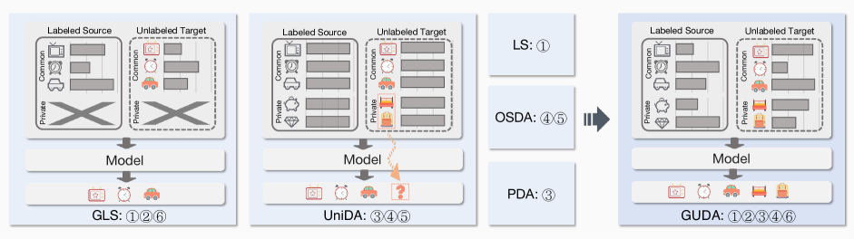
Figure 1. Illustration of GUDA and some subproblems of GUDA. GUDA contains most domain adaptation tasks from the perspective of label distribution, label space and label prediction space.

Label distribution based variants mainly focus on estimating label ratio to reweight source samples, whereas label space based variants aim to design heuristic rules to determine whether the samples belong to the private label set. However, methods for these two types of variants are incapable of resolving one another. In practice, it is difficult to identify which variant is being encountered, and real-world scenarios may involve a combination of these variants, making it challenging to apply any single method. Furthermore, the label space based variants can only identify unseen categories as "unknown", limiting their ability to achieve fine-grained recognition. These dilemmas highlight the necessity for a unified framework to address both label distribution and label space variants, while also enabling precise prediction of unknown categories.

In this paper, we propose a new problem Generalized Universal Domain Adaptation (GUDA) to take a unified view of these above problems, as illustrated in Fig. 1, which can be represented as ① $\wedge$ ② $\wedge$ ③ $\wedge$ ④ $\wedge$ ⑥. The key challenge of GUDA is developing and identifying novel categories that exist in the target domain while estimating the overall label distribution for subsequent feature alignment. To address GUDA, we take the benefit of the powerful exploration capability of Generative Flow Networks (GFlowNets) (Bengio et al., 2021b) and propose an active domain adaptation framework named GFlowDA,  which could explore the overall target label distribution by annotating a subset of target data. Unlike the previous active domain adaptation (ADA) works (Fu et al., 2021; Prabhu et al., 2021; Xie et al., 2022b; Ma et al., 2021; Hwang et al., 2022; Xie et al., 2022a; de Mathelin et al., 2021), which either focus on designing metrics (Ma et al., 2021; Fu et al., 2020; Xie et al., 2022a) that may have some bias or minimizing the feature distance while easily falling into the trap of sub-optimal solutions (Hwang et al., 2022; de Mathelin et al., 2021; Prabhu et al., 2021; Xie et al., 2022b), our insight is to learn a generative policy that generates a distribution with probabilities proportional to the distance of the original target distribution. We consider the selected target subset as a compositional object and formulate the ADA problem as a distribution generative process by sequentially selecting a target sample through GFlowNets. To facilitate GFlowNets to better perceive the target label distribution, we customize the states and rewards, and introduce an efficent parent exploration and state transition approach. Finally, we propose a weighted adaptive model named Generalized Universal Adversarial Network (GUAN), which enables efficient domain alignment through a reciprocal relationship between GFlowNets and GUAN.

Main Contribution: (1) We introduce GUDA, which covers most UDA variants with label heterogeneity and aims to recognize all target classes including unknown classes. (2) To address this challenge, we propose GFlowDA to select and annotate target samples to estimate the overall target label distribution. (3) We define the design paradigm for states and rewards, and introduce an efficient solution for parent exploration and state transition in the GFlowDA training process. We also propose a new training paradigm called GUAN, which involves collaborative optimization between GUAN and GFlowNet. (4) Theoretical analysis and extensive experiments show that the effectiveness of our GFlowDA.

2. Related Works

2.1. Unsupervised Domain Adaptation

For LS and GLS problems in the literature of UDA, most works  (Tachet des Combes et al., 2020; Shui et al., 2021; Le et al., 2021; Kirchmeyer et al., 2021; Rakotomamonjy et al., 2022; Zhao et al., 2019) seek to estimate the label ratio $P_{t}(Y)/P_{s}(Y)$ to weight the source feature, which requires that the source label distribution $P_{s}(Y)$ cannot be zero. This underlying constraint limits the generalization of the methods for LS and GLS to OSDA (Saito et al., 2018b; Panareda Busto and Gall, 2017) and UniDA (You et al., 2019) scenarios due to the existence of target private labels. Numerous methods for OSDA and UniDA either utilize prediction uncertainty (Saito et al., 2018a; You et al., 2019; Fu et al., 2020; Lifshitz and Wolf, 2020; Saito and Saenko, 2021; Tao et al., 2023; Ma et al., 2022), or incorporate self-supervised learning techniques (Baktashmotlagh et al., 2018; Saito et al., 2020; Li et al., 2021; Zhu et al., 2023; Tong et al., 2023). However, these methods often fail to explore fine-grained discriminative knowledge in the unknown set and do not take label distribution shift into account within the common label space. Additionally, most PDA methods (Cao et al., 2018; Zhang et al., 2018; Liang et al., 2020) aim to weight source samples with heuristic criteria, which suffe from the same limitations as OSDA and UniDA. While recent methods such as OSLS (Garg et al., 2022) and AUDA (Ma et al., 2021) attempt to address some of the above limitations, they may not be suitable for GUDA. Further research is needed to develop more effective methods that can overcome the challenges posed by GUDA.

2.2. Generative Flow Networks

GFlowNets (Bengio et al., 2021a) is a generative model which aims to solve the problem of generating diverse candidates. It has been effective in various fields such as molecule generation (Bengio et al., 2021b; Malkin et al., 2022), discrete probabilistic modeling (Zhang et al., 2022f), graph neural networks (Li et al., 2023a, b) and causal discovery (Li et al., 2022a). Another research direction aims to address and extend the inherent assumptions of the original GFlowNet (Li et al., 2023d, 2022b, c; Wang et al., 2023). Compared to reinforcement learning (RL) methods (Sutton and Barto, 2018), which focus on maximizing the expected return by generating a sequence of actions with the highest reward, GFlowNets offer the ability to explore diverse reward distributions by sampling trajectories with probabilities proportional to the expected rewards. This feature allows for more effective estimation of the target distribution.

2.3. Active Domain Adaptation

The pioneering study  (Rai et al., 2010) demonstrates how active learning (AL) and DA can collaborate to enhance AL in DA. Recent efforts  (Su et al., 2020; Fu et al., 2021; Xie et al., 2022b) design some criterion by introducing advanced techniques like adversarial training, multiple discriminators and free energy model. Besides, some parallel works (Prabhu et al., 2021; Ma et al., 2021) suggest using clustering to choose samples. In addition, distance-based works (de Mathelin et al., 2021; Hwang et al., 2022; Xie et al., 2022a; Prabhu et al., 2021; Ma et al., 2021; Yuan et al., 2022) choose samples based on their distance to the source or the target domain. Overall, existing works mainly rely on manually-designed criteria or distance, leading to overfitting to specific scenarios and easily falling into sub-optimal solutions. Unlike the existing ADA methods, we consider the query batch as a compositional object and formulate the ADA as a generative process. The generative policy network can automatically explore how to find the most informative samples in an essential way.

3. Problem Formulation

Denoting $\mathcal{X}$, $\mathcal{Y}$, $\mathcal{Z}$ as the input space, label space and latent space, respectively. Let $X$, $Y$ and $Z$ be the random variables of $\mathcal{X}$, $\mathcal{Y}$, $\mathcal{Z}$, and $x$, $y$ and $z$ be their respective elements. Let $P_{s}$ and $P_{t}$ be the source distribution and target distribution. We are given a labeled source domain $\mathcal{D}_{s}=\{{x}_{i},{y}_{i})\}_{i=1}^{m}$ and an unlabeled target domain $\mathcal{D}_{t}=\{{x}_{i}\}_{i=1}^{n}$ are respectively sampled from $P_{s}$ and $P_{t}$, where $m$ and $n$ denote the numbers of source samples and target samples. Denote $\mathcal{Y}_{s}$ and $\mathcal{Y}_{t}$ as the label sets of the source and target domains, respectively. Suppose the feature transformation function is $g:\mathcal{X}\rightarrow\mathcal{Z}\subseteq\mathbb{R}^{d_{z}}$ where $d_{z}$ is the length of each feature vector, and the discrimination function of the label classifier is $h:\mathcal{Z}\rightarrow\mathcal{Y}$.

Given $\mathcal{Y}_{c}=\{1,2,\dots,k\}$ as the common label space between the source and target domain. We denote $\overline{\mathcal{Y}}_{t}=\{k+1,\dots,k+n\}$ as the target private label space and $\overline{\mathcal{Y}}_{s}$ the source private label space, i.e., $\mathcal{Y}_{s}=\mathcal{Y}_{c}\cup\overline{\mathcal{Y}}_{s},~{}\mathcal{Y}_{t}=\mathcal{Y}_{c}\cup\overline{\mathcal{Y}}_{t}$. Then we have GUDA in Definition 1.

Definition 0 (GUDA).

GUDA is characterized by conditions ① $\wedge$ ② $\wedge$ ③ $\wedge$ ④ $\wedge$ ⑥, i.e.,

(1) $$P_{s}(X|Y) \neq P_{t}(X|Y)>0,~{}P_{s}(Y)\neq P_{t}(Y)>0,~{}\exists Y\in\mathcal{Y}_{c},$$

and $$\quad\overline{\mathcal{Y}}_{s}\neq\emptyset,\quad\overline{\mathcal{Y}}_{t}\neq\emptyset,\quad|\widehat{\mathcal{Y}}|=k+n,$$

where $\overline{\mathcal{Y}}_{s}$ and $\overline{\mathcal{Y}}_{t}$ are both unknown.

GUDA focuses on predicting all target labels, including the private label set, while also accounting for unknown label spaces and generalized label shift. Therefore, the target risk of GUDA can be divided into two parts: the target common risk for classifying common classes and the refined target private risk for classifying the target private classes:

(2) $$\epsilon_{t}({h}\circ g)=\mathbb{E}_{({X},{Y})\sim\mathcal{D}_{t}}\ell({h}\circ g({X}),{Y})$$

$$=\underbrace{\sum_{i=1}^{k}P_{t}(Y=i)\epsilon_{s,i}(h\circ g)}_{\text{target common risk}}+\underbrace{\sum_{j=k+1}^{k+n}P_{t}(Y=j)\epsilon_{s,j}(h\circ g)}_{\text{refined target private risk}}.$$

To minimize the target risk, an AL strategy can be employed to annotate a small portion of the target dataset to recover the target distribution. We denote $\mathcal{D}_{l}={(x_{i},y_{i})}_{i=1}^{b}$ as the selected labeled target dataset and the probability distribution of $\mathcal{D}_{l}$ as $P_{l}$.

4. Method

4.1. Towards GUDA from a Theoretical View

To start with, we provide a theoretical analysis of the proposed GUDA. First, we introduce the definitions of two performance metrics for the predictor $h\circ g$:

Definition 0 (Balanced Error Rate (Tachet des Combes et al., 2020)).

Given a distribution $P_{s}$, the balanced error rate (BER) of a predictor $h\circ g$ on $P_{s}$ is given by:

$$\varepsilon_{s}(\widehat{Y}||Y):=\max_{j\in\mathcal{Y}}P_{s}(\widehat{Y}\neq Y\mid Y=j),$$

where $\widehat{Y}=h\circ g(X)$.

Definition 0 (Conditional Error Gap (Tachet des Combes et al., 2020)).

Given two distributions $P_{s}$ and $P_{t}$, the conditional error gap (CEG) of a classifier $h\circ g$ on $P_{s}$ and $P_{t}$ is given by

$$\Delta_{s,t}(\widehat{Y}||Y):=\max_{j\neq i\in\mathcal{Y}}|{P}_{s}(\widehat{Y}=i|Y=j)-{P}_{t}(\widehat{Y}=i|Y=j)|.$$

BER measures max prediction error on $P_{s}$, reflecting the classification performance of a single domain. CEG characterizes the max discrepancy between the classifier’s predictions on $P_{s}$ and $P_{t}$, reflecting the degree of conditional feature alignment across domains.

Then we present the target risk upper bound for GUDA in Theorem 3 based on these two definitions, proved in the appendix.

Theorem 3 (Target Risk Upper Bound for GUDA).

Let $Y_{c}$, $Y_{l}$ and $\overline{Y}_{t}$ be random variables taking values from $\mathcal{Y}_{c}$, $\mathcal{Y}_{l}$ and $\overline{\mathcal{Y}}_{t}$ respectively, with $\mathcal{Y}_{l}$ being the selected target label space. For any classifier $\widehat{Y}=(h\circ g)(X)$, we have

$$\epsilon_{t}(h\circ g)\leq\epsilon_{s}(h\circ g)+\epsilon_{l}(h\circ g)+\delta_{s,t}+\delta_{l,t}+\varepsilon_{{t}}(\widehat{Y}||\overline{Y}_{t}),$$

where

$$\delta_{s,t} =\left\|P_{s}(Y_{c})-P_{t}(Y_{c})\right\|_{1}\cdot\varepsilon_{{s}}(\widehat{Y}||Y_{c})+2(k-1)\Delta_{{s},t}(\widehat{Y}||Y_{c}),$$

$$\delta_{l,t} =\left\|P_{l}(Y_{l})-P_{t}(Y_{l})\right\|_{1}\cdot\varepsilon_{{l}}(\widehat{Y}||{Y}_{l})+2(v-1)\Delta_{{l},t}(\widehat{Y}||Y_{l})$$

with $k=|\mathcal{Y}_{c}|$ and $v=|\mathcal{Y}_{l}|$, $\|{P}_{s}(Y_{c})-{P}_{t}(Y_{c})\|_{1}=\sum_{i\in\mathcal{Y}_{c}}|P_{s}(Y=i)$ $-P_{t}(Y=i)|$ being the $L_{1}$ distance between $P_{s}(Y)$ and $P_{t}(Y)$ on the common label space $\mathcal{Y}_{c}$.

Remark 1.

The upper bound $\epsilon_{t}(h\circ g)$ contains five terms. The first two terms represent the source risk on $\mathcal{Y}_{c}$ and the selected target risk on $\mathcal{Y}_{l}$. The third and fourth terms contain $\|{P}_{s}(Y_{c})-{P}_{t}(Y_{c})\|_{1}$ and $\|{P}_{l}(Y_{l})-{P}_{t}(Y_{l})\|_{1}$ respectively, which both measure the distances of the marginal label distributions across domains. The former is a constant that only depends on $\mathcal{D}_{s}$ and $\mathcal{D}_{t}$ while the latter changes dynamically since the construction of $\mathcal{D}_{l}$ varies with the AL strategy. $\varepsilon_{a}(\cdot)$ with $a\in\{s,l,t\}$ in the last three terms measure classification performance on the corresponding domains. $\Delta_{a,t}(\cdot)$ with $a\in\{s,l\}$ in the third and fourth terms measures the performance discrepancy between $P_{a}(Y)$ and $P_{t}(Y)$.

The difficulty in minimizing the upper bound stems from the unknown nature of the target label distribution $P_{t}(Y_{t})$ and the label space $\mathcal{Y}_{t}$. One potential solution is to minimize the label distribution distance $|P_{l}(Y_{l})-P_{t}(Y_{l})|_{1}$ while making $|\mathcal{Y}_{l}|$ close to $|\mathcal{Y}_{t}|$. To achieve this goal, it is crucial to develop an effective AL strategy to select informative and representative samples for constructing $\mathcal{D}_{l}$ that preserves the entire target label distribution and label space. By doing so, $\mathcal{Y}_{l}$ can be considered a proxy of $\mathcal{Y}_{t}$ and $P_{l}$ a proxy of $P_{t}$. We propose GFlowDA based on a GFlowNet generator to generate $\mathcal{D}_{l}$ by sequentially adding one sample at each step until the budget is used up. We give the formal definition of GFlowDA in Definition  4.

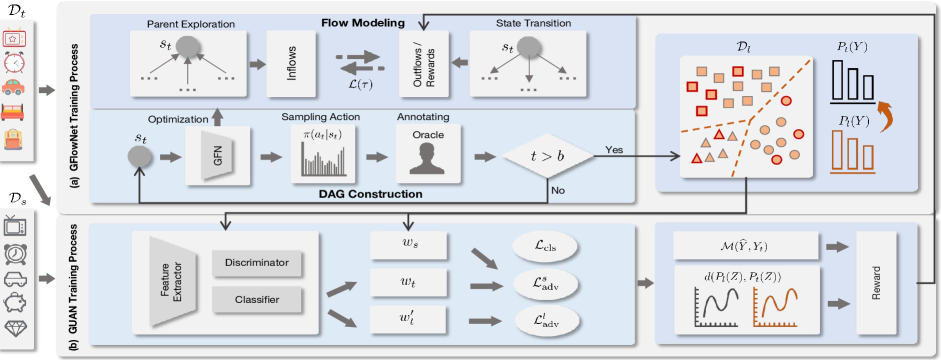
Figure 2. Overall framework of GFlowDA. GFlowNet selects and labels target samples, which are then fed as $\mathcal{D}_{l}$ to GUAN. GUAN is optimized based on $\mathcal{D}_{l}$, $\mathcal{D}_{s}$ and $\mathcal{D}_{t}$. The resulting reward is fed back to GFlowNet, which is then optimized by combining the reward with the inflows and outflows obtained through the parent exploration and state transition process.

Definition 0 (GFlowDA).

Given a source distribution ${P}_{s}$ and a target distribution ${P_{t}}$, GFlowDA aims to find the best forward generative policy $\pi(\theta)$ based on flow network to generate a distribution $P_{l}$ automatically, which can serve as a proxy of $P_{t}$. The probability of sampling the distribution $P_{l}$ satisfies

(3) $$\pi(P_{l};\theta)\propto r(P_{s},P_{t},P_{l}),$$

where $\theta$ is the parameter of flow network, $r(\cdot)$ is the reward function based on $P_{s}$, $P_{t}$ and $P_{l}$.

4.2. DAG Construction of GFlowDA

Consider a direct acyclic graph (DAG) $\mathcal{G}=(\mathcal{S},\mathcal{A})$, where $\mathcal{S}$ and $\mathcal{A}$ are state/node and action/edge sets, respectively. Elements of them at step $t$ are denoted as $s_{t}$ and $a_{t}$ The complete trajectory is a sequence of states $\tau=(s_{0},\ldots,s_{f})$. To construct $\mathcal{G}$, we first define the state, action and reward function.

Definition 0 (State).

A state $s_{t}\in\mathcal{S}\subseteq\mathbb{R}^{n\times 4}$ in GFlowDA at step $t$ describes the entire target information based on $\mathcal{D}_{t}$ and the currently labeled data $\mathcal{D}_{l}$, where $s_{t}=\{s_{t}^{i}\}_{i=1}^{n}$ and $s_{t}^{i}$ is the state representation of the $i$-th target sample.

We use $s^{i}_{t}(a),a\in\{0,1,2,3\}$ denotes the $a$-th column of the state matrix. The first column of the state denotes the maximum similarity between target features and selected target features at step $t$. Intuitively, selecting samples with low maximum similarity values can ensure the instance-level diversity, i.e.,

(4) $$s^{i}_{t}(1)=\operatorname{max}_{x_{j}\in\mathcal{D}_{l}}\operatorname{cos}(g(x_{i}),g(x_{j})).$$

The second column of the state denotes the maximum similarity between target features and active target prototypes, which ensures class-level diversity, i.e.,

(5) $$s^{i}_{t}(2)=\operatorname{max}_{j\in\mathcal{Y}_{l}}\operatorname{cos}(g(x_{i}),{\mu_{l}^{j}}),$$

where $\mu_{l}^{j}$ is the prototype of class $j$ in $\mathcal{D}_{l}$, calculated as follows:

(6) $$\mu_{l}^{j}=\frac{\sum_{(x,y)\in\mathcal{D}_{l}}\mathds{1}\{y=j\}g({x})}{\sum_{(x,y)\in\mathcal{D}_{l}}\mathds{1}\{y=j\}}.$$

The third column of the state denotes the uncertainty of the target samples, which is calculated by the entropy of the label probabilities $\hat{y}_{i}=h\circ g(x_{i})$, i.e.,

(7) $$s^{i}_{t}(3)=H(\hat{y}_{i})).$$

The last column of the state is an indicator variable to represent whether a sample has been labeled or not, i.e.,

(8) $$s^{i}_{t}(4)=\mathds{1}\{x_{i}\in\mathcal{D}_{l}\}.$$

Definition 0 (Action).

An action $a_{t}\in\mathcal{A}$ at step $t$ in GFlowDA determines which target instance will be selected from candidate target dataset $\mathcal{D}_{t}\backslash\mathcal{D}_{l}$.

Definition 0 (Reward Function).

A reward function $r(s_{f})$ of the terminal state $s_{f}$ in GFlowDA refers to a comprehensive metric measuring the quality of $\mathcal{D}_{l}$, by taking into account the diversity and informativeness, which is expressed as:

(9) $$r(s_{f})= -\operatorname{MMD}(g(X_{t}),g(X_{l})+\mathcal{M}(\widehat{Y},Y_{t}),$$

where $\widehat{Y}=h\circ g(X)$, $\operatorname{MMD}(\cdot)$ represents the Maximum Mean Discrepancy (MMD) (Long et al., 2017) between the source and target marginal feature, and $\mathcal{M}(\cdot)$ means the classification accuracy used to evaluate the performance of $h\circ g$.

Remark 2.

MMD distance can encourage diverse sample selection that preserves the entire target distribution. To make the selected samples more informative, we incorporate the classification accuracy of the model on the target domain as part of the reward.

4.3. Flow Modeling of GFlowDA

To achieve Eq. 3, a non-negative function $F(\cdot)$ is introduced to measure the probabilities associated with $s_{t}$, where $F(s_{t},a_{t})=F(s_{t}\rightarrow s_{t+1})$ corresponds to an action/edge flow. The trajectory flow is denoted as $F(\tau)$ and the state flow is the sum of all trajectory flows passing through that state, denoted as $F(s)=\sum_{s\in\tau}F(\tau)$. Our objective is to ensure that the DAG $\mathcal{G}$ operates analogously as a water pipe, where water enters at $s_{0}$ and flows out through all $s_{f}$, satisfying the condition $F(s_{0})=\sum F(s_{f})=\sum r(s_{f})$. To achieve this, we need to calculate the inflows and outflows of each state, corresponding to the parent exploration and state transition, respectively. As illustrated in Fig. 3, in the parent exploration process, we explore all direct parent states of $s_{t}$, i.e., $s\in\mathcal{S}_{p}(s_{t})$ with $\mathcal{S}_{p}(s_{t})$ being the parent set. We have the following proposition to guide the exploration procedure:

Proposition 0.

For a state $s_{t}$ in GFlowDA, the number of its parent nodes is equal to the number of labeled samples currently, i.e., $|\mathcal{S}_{p}(s_{t})|=||s_{t}(4)||_{0}$.

Based on Proposition 8, one of $s_{t}$’s parents is obtained by three steps: (a) selecting the $j$-th element in the vector $s_{t}(4)$ and setting its value from $1$ to $0$ to obtain a new vector $s_{t-1}(4)$, (b) updating the instance-level similarity and (c) updating the class-level similarity based on $s_{t-1}(4)$. Notably, $s_{t}(3)$ remains fixed as the domain adaptation model updates only at the terminal state. However, directly computing all parent states using Eq.4 and Eq.5 is too time-consuming. Therefore, we propose a more efficient approach to update the similarities. For instance-level similarity, we pre-calculate a cosine similarity matrix $\text{SIM}(X_{t})$ between all target domain samples at the start of the generative process. The state of the $i$-th target sample in the first column can be updated as follows.

(10) $$s_{t-1}^{i}(1)=\max(s^{i}_{t}(1),\text{SIM}_{i,j}),$$

where $\text{SIM}_{i,j}$ denotes the similarity between the $i$-th target sample and the $j$-th target sample. For class-level similarity, we just need to update $\mu_{t}^{c}$ with $c$ being the label of the selected $j$-th sample. $\mu_{t-1}^{c}$ can be quickly calculated based on $\mu_{t}^{c}$, which is given by

(11) $$\mu_{t-1}^{c}=\frac{\mu_{t}^{c}\cdot(\sum_{{x}\in\mathcal{D}_{l}}\mathds{1}\{y=c\})-g(x_{j})}{\sum_{{x}\in\mathcal{D}_{l}}\mathds{1}\{y=c\}-1}.$$

Then the state of the $i$-th target sample in the second column can be updated as follows:

(12) $$s_{t-1}^{i}(2)=\max(s^{i}_{t}(2),\cos(\mu_{t-1}^{c},x_{i})).$$

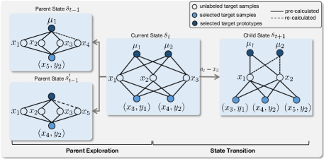
Figure 3. Illustration of efficient parent exploration and state transition. Left: At state $s_{t}$, $x_{3}$ and $x_{4}$ are labeled as $y_{1}$ and $y_{2}$, resulting in two parent states. Right: Due to $a_{t}=x_{3}$ , $x_{3}$ is labeled at $s_{t+1}$, and the prototype $\mu_{2}$ needs to be updated.

In the state transition process, if $s_{t}$ is not a terminal state, we update the dynamic features of $s_{t}$ to obtain its child state $s_{t+1}$. This process can be considered an inverse repetition of the parent exploration process. Specifically, once $a_{t}=j$ is sampled, the $j$-th element in vector $s_{t}(4)$ is updated from $0$ to $1$, resulting in a new vector $s_{t+1}(4)$. Based on $s_{t+1}(4)$,$s_{t+1}(1)$ can be updated by utilizing Eq. 10. To update $s_{t+1}(2)$, we use a similar equation as Eq.12. Since we need to add a new sample instead of removing one as in Eq.11, $\mu_{t+1}^{c}$ is updated as follows:

(13) $$\mu_{t+1}^{c}=\frac{\mu_{t+1}^{c}\cdot(\sum_{{x}\in\mathcal{D}_{l}}\mathds{1}\{y=c\})+g(x_{j})}{\sum_{{x}\in\mathcal{D}_{l}}\mathds{1}\{y=k\}+1}.$$

Overall, efficient exploration reduces complexity and accelerates the training of the generative policy network with flow matching loss (discussed in the next subsection).

4.4. Training Procedure

As illustrated in Fig. 2, GFlowDA consists of two primary components: a generative policy network for selecting and annotating the most useful target samples, and a domain adaptation network that utilizes the annotated samples to adapt the target domain.

Genrative Policy Network. Based on the parent set $\mathcal{S}_{p}(s_{t})$ and child set $\mathcal{S}_{c}(s_{t})$ obtained through the above exploration and transition process, we can calculate the corresponding inflows and outflows. The inflows are calculated by $\sum_{s\in\mathcal{S}_{p}(s_{t})}F(s)$, which represents the sum of action flows from all parent states. The outflows are flows passing through it, which is given by $\sum_{s\in\mathcal{S}_{c}(s_{t})}F(s)$. Starting from an empty set, GFlowDA draws complete trajectories $\tau=(s_{0},s_{1},\ldots,s_{f})$ by iteratively sampling target samples until the budget is used up. After sampling a buffer, we train the policy $\pi(\theta)$ to satisfy Eq. 3, by minimizing the loss over the flow matching condition:

(14) $$\mathcal{L}(\tau)=\sum_{s_{t}\in\tau\neq s_{0}}\Bigg{\{}\log\bigg{[}\epsilon+\sum_{s\in\mathcal{S}_{p}(s_{t})}F^{\prime}\bigg{]}$$

$$-\log\bigg{[}\epsilon+\mathds{1}_{s_{t}=s_{f}}r\left(s_{f}\right)+\mathds{1}_{s_{t}\neq s_{f}}\sum_{s\in\mathcal{S}_{c}(s_{t})}F^{\prime}\bigg{]}\Bigg{\}}^{2},$$

where $F^{\prime}=\exp(\log F(s)$), and the reward $r(s_{f})$ is computed by Eq. 9. For internal states, we only calculate outflows based on action distributions. For terminal states, we calculate their rewards to evaluate the efficacy of $\mathcal{D}_{l}$. To acquire a dependable reward, we introduce a new domain adaptation network as follows.

Table 1. Average class accuracies (%) and JSD (%) on Office-31 with 5% target data as the labeling budget.

Method	A $\rightarrow$ D		A $\rightarrow$ W		D $\rightarrow$ A		D $\rightarrow$ W		W $\rightarrow$ A		W $\rightarrow$ D		Avg
	Acc	JSD	Acc	JSD	Acc	JSD	Acc	JSD	Acc	JSD	Acc	JSD	Acc	JSD
Random	46.23	16.22	60.79	15.80	55.67	3.14	67.98	14.39	61.80	3.57	67.46	15.64	59.99	11.46
Entropy (Wang and Shang, 2014)	53.85	27.93	57.12	23.53	65.88	15.09	70.12	22.96	67.16	4.93	70.91	35.04	64.17	21.58
TQS (Fu et al., 2021)	63.10	16.02	67.80	15.92	65.72	2.67	82.40	16.84	66.85	3.01	80.65	21.93	71.09	12.73
CLUE (Prabhu et al., 2021)	56.89	23.96	66.12	15.36	61.01	3.97	81.37	16.39	60.13	7.23	75.27	22.06	66.80	14.83
EADA (Xie et al., 2022b)	46.63	27.15	65.40	21.10	51.05	7.60	72.40	28.39	54.22	7.11	73.02	22.93	60.45	19.05
SDM-AG (Xie et al., 2022a)	62.76	22.85	68.20	17.38	65.3	5.67	79.40	21.42	64.41	3.49	72.43	25.87	68.75	16.11
AUDA (Xie et al., 2022b)	65.13	21.36	67.36	18.32	67.12	5.01	79.60	20.87	63.78	4.12	77.14	19.36	70.02	14.84
RLADA (Ours)	67.36	20.33	71.23	16.79	70.56	3.67	79.88	16.03	65.98	3.20	76.78	19.66	71.96	13.28
GFlowDA (Ours)	70.50	15.01	73.00	13.54	74.80	1.72	82.60	11.93	67.51	1.51	80.75	14.40	74.86	9.68

Table 2. Average class accuracies (%) and JSD (%) on Office-Home with 5% target data as the labeling budget.

Method	Ar$\rightarrow$ Cl		Ar$\rightarrow$ Pr		Ar$\rightarrow$ Rw		Cl$\rightarrow$ Ar		Cl$\rightarrow$ Pr		Cl$\rightarrow$ Rw		Avg (12 tasks)
	Acc	JSD	Acc	JSD	Acc	JSD	Acc	JSD	Acc	JSD	Acc	JSD	Acc	JSD
Random	38.80	7.24	63.92	6.06	63.67	6.91	42.38	12.14	61.69	5.47	65.48	5.40	52.20	7.76
Entropy (Wang and Shang, 2014)	37.39	8.79	65.79	7.20	57.75	22.09	38.52	14.70	56.22	10.92	55.37	12.49	48.36	14.72
TQS (Fu et al., 2021)	43.55	6.15	68.94	8.38	64.47	5.37	39.39	11.37	59.63	6.12	54.00	7.74	52.49	8.04
CLUE (Prabhu et al., 2021)	42.14	7.12	70.12	5.88	65.12	4.78	41.57	7.54	63.11	7.23	56.23	7.17	53.98	7.16
EADA (Xie et al., 2022b)	40.36	5.65	69.06	7.44	62.19	6.17	30.67	10.68	65.14	9.47	54.53	7.64	50.28	9.32
SDM-AG (Xie et al., 2022a)	40.01	8.43	69.25	7.99	62.26	8.54	38.21	9.74	53.13	10.98	51.51	9.78	42.84	10.83
LAMDA (Hwang et al., 2022)	42.19	8.59	59.75	7.22	70.51	9.25	44.80	17.49	67.17	6.21	52.47	10.21	53.86	11.37
RLADA (Ours)	47.56	7.12	72.69	6.73	65.81	7.33	40.37	10.67	66.52	8.64	60.46	6.48	55.32	7.68
GFlowDA (Ours)	51.89	5.01	74.77	4.87	72.99	5.46	44.23	7.12	72.29	6.18	67.11	5.03	59.32	5.65

Generalized Universal Adversarial Network. In the GFlowDA framework, we propose a novel weighted adaptive model for GUDA named Generalized Universal Adversarial Network (GUAN). In addition to the feature extractor $g$ and classifier $h$, GUAN also includes a domain discriminator $d:\mathcal{Z}\rightarrow\mathbb{R}$, which aims to align the source and target features adversarially. The weighted alignment losses of source data and labeled target data are formally described as follows

(15) $$\mathcal{L}^{s}_{\text{adv}}=-\mathbb{E}_{x\sim P_{s}}{w}_{s}\log\left(d(z)\right)-\mathbb{E}_{x\sim P_{t}}{w}_{t}\log\left(1-d(z)\right)$$

(16) $$\mathcal{L}^{l}_{\text{adv}}=-\mathbb{E}_{x\sim P_{l}}\log\left(d(z)\right)-\mathbb{E}_{x\sim P_{t}}{w}^{\prime}_{t}\log\left(1-d(z)\right),$$

where $z=g(x)$. $w_{s}$ in Eq. 15 indicates the ratio between the estimated target label distribution and the source label distribution if $x$ is determined to belong to $\mathcal{Y}_{c}$, which is defined as follows:

$${w}_{s}=\mathds{1}(y\in\mathcal{Y}^{\prime})\cdot(P_{l}(y)/P_{s}(y))+(1-\mathds{1}(y\in\mathcal{Y}^{\prime}))\cdot\lambda$$

where $\mathcal{Y}^{\prime}=\mathcal{Y}_{l}\cap\mathcal{Y}_{s}$ acting as an approximation of the common label space $\mathcal{Y}_{c}$, and $\lambda$ is a constant working as a remedy for compatibility with the potential inconsistency between $\mathcal{Y}^{\prime}$ and $\mathcal{Y}_{c}$.

$w_{t}({x})$ in Eq. 15 and $w^{\prime}_{t}({x})$ in Eq. 16 indicate the probability of a target sample ${x}$ belonging to the source label set $\mathcal{Y}_{s}$ and the selected labeled target label set $\mathcal{Y}_{l}$, respectively. We use the predicted probabilities over all labels in $\mathcal{Y}_{s}$ and $\mathcal{Y}_{l}$ respectively to estimate the probabilities, as described below:

(17) $${w}_{t}=\frac{1}{u}\sum_{i\in\mathcal{Y}_{s}}\hat{\bm{y}}[i],\quad{w}^{\prime}_{t}=\frac{1}{v}\sum_{i\in\mathcal{Y}_{l}}\hat{\bm{y}}[i]$$

where $k=|\mathcal{Y}_{c}|$ and $v=|\mathcal{Y}_{l}|$, $\hat{\bm{y}}=h(z)$ represents the prediction probability vector.

The classification loss for GUAN aims to minimize the cross-entropy loss for both source and labeled target samples:

(18) $$\mathcal{L}_{\text{cls}}= -\mathbb{E}_{x\sim P_{s}}L\left(\hat{y},{y}\right)-\mathbb{E}_{x\sim P_{l}}L\left(\hat{y},y\right),$$

where $\hat{y}=h\circ g\left(x\right)$ and $L(\cdot)$ is the cross entropy loss.

5. Experiments

5.1. Experimental Setup

Datasets. We perform experiments on five benchmarks including Office-31 (Saenko et al., 2010), Office-Home (Venkateswara et al., 2017), PACS (Li et al., 2017) and VisDA (Peng et al., 2018). To evaluate our algorithm on GUDA, we modify the source and target dataset by combining two subsampling protocols  (You et al., 2019; Tachet des Combes et al., 2020). These protocols are tailored for GLS and UniDA respectively. See the appendix for more details.

Table 3. Average class accuracies (%) and JSD (%) on PACS and with 1% target data as the labeling budget.

Method	PACS (%)												VisDA (%)
	A $\rightarrow$ C		A $\rightarrow$ P		A $\rightarrow$ S		C $\rightarrow$ A		C $\rightarrow$ P		Avg (12 tasks)		S$\rightarrow$ R
	Acc	JSD	Acc	JSD	Acc	JSD	Acc	JSD	Acc	JSD	Acc	JSD	Acc	JSD
Random	52.80	0.29	81.86	9.69	60.24	1.58	58.35	0.02	82.80	11.98	63.27	4.30	55.52	0.46
Entropy (Wang and Shang, 2014)	44.53	3.05	67.01	15.58	60.65	1.42	35.71	5.99	84.44	16.94	58.38	8.20	50.45	8.42
TQS (Fu et al., 2021)	63.82	5.82	83.89	5.71	80.43	2.77	44.48	4.39	87.65	3.47	63.12	6.37	82.87	5.10
EADA (Xie et al., 2022b)	35.18	9.01	28.46	34.67	38.21	5.42	23.97	7.67	40.66	26.67	34.38	11.16	84.73	1.98
SDM-AG (Xie et al., 2022a)	68.76	3.91	90.63	7.81	84.03	2.39	51.63	2.55	74.90	6.73	63.16	4.18	80.69	2.60
LAMDA (Hwang et al., 2022)	53.20	1.62	82.67	6.66	55.87	2.96	58.81	1.04	91.08	9.81	65.97	5.85	-	-
RLADA (Ours)	59.78	3.28	90.12	4.32	67.03	0.80	57.03	2.78	87.21	4.07	66.00	2.94	81.23	3.23
GFlowDA (Ours)	64.34	1.06	91.38	4.11	67.23	0.55	56.66	0.61	90.54	1.87	68.26	1.93	85.23	1.03

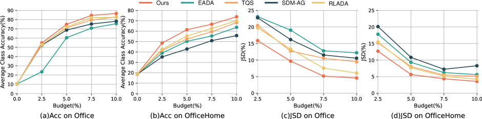
Figure 4. Average class accuracies (%) and JSD (%) on Office-31 and Office-Home with different budget.

Evaluation metrics. Besides reporting the average class accuracy, we also compared the Jensen-Shanon divergence (JSD) between the label distribution of the selected samples and the original target samples, denoted by $d_{\text{JS}}(P_{l}^{Y},P_{t}^{Y})$. JSD can provide an intuitive reflection of the label distribution reduction and exploration ability of AL strategies. A smaller JSD value indicates that the selected samples are better able to estimate the original distribution. Compared baselines and Implementation details are introduced in Sec B.2 and Sec B.3 in the Appendix.

5.2. Main Results of GFlowDA

Performance of GFlowDA on GUDA. The experimental results of different methods on Office-31, Office-Home, PACS and VisDA are shown in Table 1, Table 2 and Table 3 respectively, demonstrating that GFlowDA surpasses all the baselines by a large margin in both accuracy and JSD. It is worth noting that the random strategy outperforms most heuristic rule-based methods in terms of JSD, which is statistically intuitive that random selection is an independent and identically distributed (i.i.d.) procedure. However, random selection is unstable, which may explain why it achieves comparable JSD but 14.87% lower accuracy than GFlowDA on Office-31. Furthermore, two learning-based active strategies, GFlowDA and RLADA, achieve optimal and suboptimal accuracy on Office-31, Office-Home and PACS, indicating that such strategies have stronger exploration ability. However, it should be noted that GFlowDA can achieve better performance and exploration than RLADA.

Table 4. Comparison results on more settings and methods.

Method	Office31-Origin		OH-RUST		Office31-GUDA		OH-GUDA
	Acc	JSD	Acc	JSD	Acc	JSD	Acc	JSD
AUDA	90.43	16.32	59.43	14.85	66.53	17.35	50.35	12.10
LAMDA	89.91	15.97	61.26	13.07	70.02	14.84	53.86	11.37
GFlowDA	92.85	15.67	63.19	11.34	74.86	9.68	61.40	5.65

Transferability of GFlowDA on GUDA. The active policy network of GFlowDA is capable of effectively transferring to tasks with varying degrees of label distribution shift and label space mismatch. To prove this, we adjust the degree of label heterogeneity by controlling the JSD distance between the source and target label distribution, denoted as $d_{\text{JS}}(P_{s}^{Y},P_{t}^{Y})$. As this distance increases, DA tasks become more challenging. Fig. 7 represents the transferability of our method compared with existing ADA methods in A$\rightarrow$W on Office-31 (More results are available in the appendix). The term "GFlowDA" refers to directly loading the active policy network pre-trained on the original dataset. "GFlowDA trained" indicates that the policy model has been fine-tuned on the new tasks by training 30 epochs. Our experimental results demonstrate that GFlowDA can directly transfer to new tasks without training, and outperforms non-learning based methods in most cases. Furthermore, ‘GFlowDA trained” improves performance on specific tasks compared to ‘GFlowDA ”.

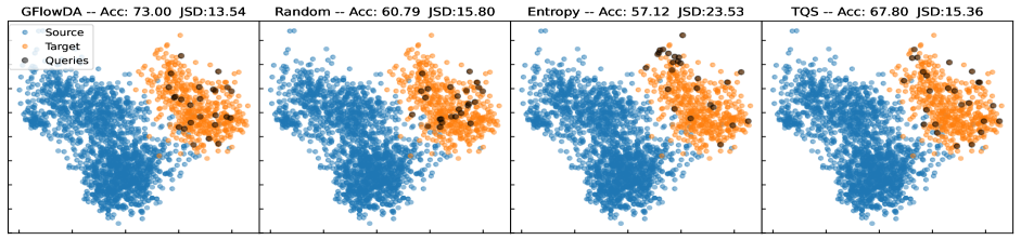
Figure 5. Feature visualization on the Office-31 A $\rightarrow$ W task. Selected samples are shown as black dots in the plots.

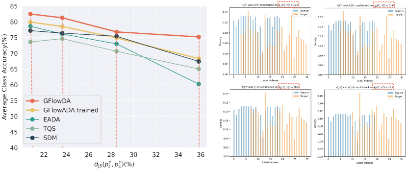
Figure 6. Left: Accuracy (%) with varying $d_{\text{JS}}(P_{s}^{Y},P_{t}^{Y})$ values. Right: Label distribution with varying $d_{\text{JS}}(P_{s}^{Y},P_{t}^{Y})$ values.

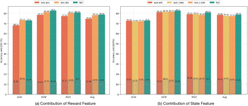
Figure 7. Ablation Study. “dis” indicates the MMD distance. “i-sim” and “c-sim” indicate instance and class-level similarity.

5.3. Further Analysis of GFlowDA

Performance of GFlowDA on Existing Settings. To demonstrate the effectiveness of GFlowDA in handling the variants included in GUDA, we evaluated its performance on Office31-Origin and OfficeHome-RUST. The former represents the original setting without label heterogeneity, while the latter represents the GLS scenario (Hwang et al., 2022). As shown in Table 4, our method outperforms or achieves comparable results to other methods.

Performance of Existing methods on GUDA. Due to the absence of AL in previous label space mismatch and label distribution shift methods, as well as differences in prediction space ($|\hat{\mathcal{Y}}|=k+1$), it is unfair and impractical to directly compare GFlowDA with those methods. To ensure fairness and gain a deeper understanding of GFlowDA, we analyze AUDA and LAMDA separately, which are AL methods developed for the UniDA and GLS settings respectively. As shown in the Tbale 4, their performance significantly decreases when applied to the GUDA setting.

Qualitative Analysis As illustrated in Fig. 5, we present the feature visualization on Office-31 A $\rightarrow$ W with 5% budget. It is obvious that the samples selected by GFlowDA can effectively restore the target label distribution, thus contributing to addressing GUDA problems. In comparison, the Random method provides a certain level of estimation for the target distribution compared to Entropy, it lacks stability and does not consider sample informativeness. The Entropy and TQS methods prioritize prediction uncertainty in sample selection, resulting in the inclusion of distant samples from the source domain. Consequently, these methods may not fully restore the target label distribution, leading to suboptimal performance.

Varying the Label Budget. To demonstrate the effectiveness of GFlowDA, we conducted experiments with varying the labeling budget from 0% to 10%, as shown in Figure 4. Across both Office-31 and Office-Home datasets, GFlowDA consistently outperforms baselines in terms of accuracy and JSD, showcasing GFlowDA can provide excellent performance across varying labeling budgets, making it a promising solution to address GUDA.

Contribution of State and Rewad Features. We further investigate the impact of the state features introduced in Section  4.2. To study how each feature affects the learned policy, we remove them from the state space individually and examine the resulting performance. The experimental results are illustrated in Figure  7 (b), which shows the performance of GFlowDA with three variants of the state on Office-31. It can be observed that removing any of the features can result in a drop in accuracy. We further analyzed the contribution of reward on GFlowDA’s performance. Figure 7 (a) shows the results. Ignoring either component would lead to a passive impact on the overall performance of GFlowDA. Overall, it is suggested that the unique combination of state and reward can effectively address GUDA.

6. Conclusion

In this work, we propose a comprehensive problem GUDA, which aims to obtain accurate predictions for unknown categories while addressing label heterogeneity. We develop an AL domain adaptation method, GFlowDA, by leveraging GFlowNets’ exploration capabilities. To achieve this, we propose a design paradigm of state and reward, along with an efficient solution for parent exploration and state transition. Additionally, GFlowDA introduces a training framework named GUAN for GUDA. Experimental results demonstrate GFlowDA’s superior performance in five benchmarks.

Appendix A Proof of Theorem 1

Before we give the proof of Theorem 3, we first present the error decomposition theorem proposed by (Tachet des Combes et al., 2020) under the assumption that $\mathcal{Y}_{s}=\mathcal{Y}_{t}$, which is stated as follows.

Theorem 1 (Error Decomposition Theorem (Tachet des Combes et al., 2020)).

For any classifier $\widehat{Y}=(h\circ g)(X)$,

$$\begin{split}&\left|\epsilon_{s}(h\circ g)-\epsilon_{t}(h\circ g)\right|\\ &\leq\left\|P_{s}(Y)-P_{t}(Y)\right\|_{1}\cdot\varepsilon_{s}(\widehat{Y}\|Y)+2(k-1)\Delta_{s,t}(\widehat{Y}\|Y).\end{split}$$

Proof of Theorem 3. Followed by (Tachet des Combes et al., 2020), we denote $\gamma_{s,j}=P_{s}(Y=j)$ for simplicity. The following identity holds for $a\in\{s,l,t\}$ by the law of total probability:

$$\epsilon_{a}(h\circ g) =\mathbb{E}_{({X},{Y})\sim P_{a}}\ell({h}\circ g({X}),{Y})$$

$$=\mathbb{E}_{({X},{Y})\sim P_{a}}P_{a}(\widehat{Y}\neq Y)$$

$$=\sum_{i\neq j}P_{a}(\widehat{Y}=i,Y=j)$$

$$=\sum_{i\neq j}\gamma_{a,j}P_{a}(\widehat{Y}=i\mid Y=j).$$

We further decompose the target risk $\epsilon_{t}(h\circ g)$ and the source risk $\epsilon_{s}(h\circ g)$ based on their common and private label space. Then we have:

$$\epsilon_{t}(h\circ g)-\epsilon_{s}(h\circ g)$$

$$= \mathbb{E}_{({X},{Y})\sim\mathcal{D}_{t}}P_{t}(Y\neq\widehat{Y})-\mathbb{E}_{({X},{Y})\sim\mathcal{D}_{s}}P_{s}(Y\neq\widehat{Y})$$

$$= \sum_{i\neq j}\gamma_{t,j}P_{t}(\widehat{Y}=i|Y=j)-\sum_{i\neq j}\gamma_{s,j}P_{s}(\widehat{Y}=i|Y=j)$$

$$\leq \left|\sum_{i\neq j,j\in\mathcal{Y}}\gamma_{t,j}P_{t}(\widehat{Y}=i|Y=j)-\sum_{i\neq j,j\in\mathcal{Y}}\gamma_{s,j}P_{s}(\widehat{Y}=i|Y=j)\right|$$

$$+ \sum_{i\neq j,j\in\overline{\mathcal{Y}}_{t}}\gamma_{t,j}P_{t}(\widehat{Y}=i|Y=j)-\sum_{i\neq j,j\in\overline{\mathcal{Y}}_{s}}\gamma_{s,j}P_{s}(\widehat{Y}=i|Y=j).$$

Based on Theorem 1, we can obtain:

$$\left|\sum_{i\neq j,j\in\mathcal{Y}_{c}}\gamma_{t,j}P_{t}(\widehat{Y}=i|Y=j)-\sum_{i\neq j,j\in\mathcal{Y}_{c}}\gamma_{s,j}P_{s}(\widehat{Y}=i|Y=j)\right|$$

$$\leq \left\|P_{s}(Y_{c})-P_{t}(Y_{c})\right\|_{1}\cdot\varepsilon_{s}(\widehat{Y}\|Y_{c})+2(k-1)\Delta_{{s},t}(\widehat{Y}\|Y_{c}),$$

Using the above inequality, we have:

$$\mathbb{E}_{({X},{Y})\sim\mathcal{D}_{t}}P_{t}(Y\neq\widehat{Y})-\mathbb{E}_{({X},{Y})\sim\mathcal{D}_{s}}P_{s}(Y\neq\widehat{Y})$$

$$\leq \left\|P_{s}(Y_{c})-P_{t}(Y_{c})\right\|_{1}\cdot\varepsilon_{s}(\widehat{Y}\|Y_{c})+2(k-1)\Delta_{{s},t}(\widehat{Y}\|Y_{c})$$

$$+ \sum_{i\neq j,j\in\overline{\mathcal{Y}}_{t}}\gamma_{t,j}P_{t}(\widehat{Y}=i|Y=j)-\sum_{i\neq j,j\in\overline{\mathcal{Y}}_{s}}\gamma_{s,j}P_{s}(\widehat{Y}=i|Y=j).$$

Recall that the source risk can be decomposed into two parts:

$$\mathbb{E}_{({X},{Y})\sim\mathcal{D}_{s}}P_{s}(Y\neq\widehat{Y})=$$

$$\sum_{i\neq j,j\in\overline{\mathcal{Y}}_{s}}\gamma_{s,j}P_{s}(\widehat{Y}=i|Y=j)+\sum_{i\neq j,j\in{\mathcal{Y}}_{c}}\gamma_{s,j}P_{s}(\widehat{Y}=i|Y=j).$$

Combining the above inequality and identity, we have:

$$\mathbb{E}_{({X},{Y})\sim\mathcal{D}_{t}}P_{t}(Y\neq\widehat{Y})$$

$$\leq \left\|P_{s}(Y)-P_{t}(Y)\right\|_{1}\cdot\varepsilon_{s}(\widehat{Y}\|Y)+2(k-1)\Delta_{{s},t}(\widehat{Y}\|Y)$$

$$+ \sum_{i\neq j,j\in\overline{\mathcal{Y}}_{t}}\gamma_{t,j}P_{t}(\widehat{Y}=i|Y=j)+\sum_{i\neq j,j\in{\mathcal{Y}_{c}}}\gamma_{s,j}P_{s}(\widehat{Y}=i|Y=j).$$

For simplicity, we still use $\epsilon_{s}(h\circ g)$ to denote the classification error on common label space, i.e., the last term of the above inequality. We have:

$$\epsilon_{t}(h\circ g)\leq\epsilon_{s}(h\circ g)$$

$$+ \left\|P_{s}(Y)-P_{t}(Y)\right\|_{1}\cdot\varepsilon_{s}(\widehat{Y}\|Y)+2(k-1)\Delta_{{s},t}(\widehat{Y}\|Y)$$

$$+ \sum_{i\neq j,j\in\overline{\mathcal{Y}}_{T}}\gamma_{t,j}P_{t}(\widehat{Y}=i|Y=j).$$

Moreover, we have

$$\sum_{i\neq j,j\in\overline{\mathcal{Y}}_{T}}\gamma_{t,j}P_{t}(\widehat{Y}=i|Y=j)\leq\varepsilon_{{t}}(\widehat{Y}||\overline{Y}_{t}),$$

where

$$\varepsilon_{t}(\widehat{Y}||\overline{Y}_{t}):=\max_{j\in\overline{\mathcal{Y}}_{t}}P_{s}(\widehat{Y}\neq Y\mid Y=j),$$

and hence,

$$\epsilon_{t}(h\circ g)\leq\epsilon_{s}(h\circ g)$$

$$+ \left\|P_{s}(Y)-P_{t}(Y)\right\|_{1}\cdot\varepsilon_{s}(\widehat{Y}\|Y)+2(k-1)\Delta_{{s},t}(\widehat{Y}\|Y)$$

$$+ \varepsilon_{{t}}(\widehat{Y}||\overline{Y}_{t}).$$

It is worth noting that the above target upper bound only involves the source domain $\mathcal{D}_{s}$. Since AL is required in GUDA, an additional domain $\mathcal{D}_{l}$ corresponding to the selecting labeled target data is introduced. Similar to the above inequality, for the error decomposition between the target and the selected labeled target domain, we have:

$$\epsilon_{t}(h\circ g)\leq\epsilon_{l}(h\circ g)$$

$$+ \left\|P_{l}(Y_{l})-P_{t}(Y_{l})\right\|_{1}\cdot\varepsilon_{l}(\widehat{Y}\|Y_{l})+2(v-1)\Delta_{{l},t}(\widehat{Y}\|Y_{l})$$

$$+ \varepsilon_{{t}}(\widehat{Y}||\overline{Y}_{t}).$$

Note that the common label space between the selected target domain $\mathcal{D}_{l}$ and the original target domain $\mathcal{D}_{t}$ is $\mathcal{Y}_{l}$ due to $\mathcal{Y}_{l}\subseteq\mathcal{Y}_{t}$. Finally, combining the above two inequalities, we get:

$$\epsilon_{t}(h\circ g)\leq\epsilon_{s}(h\circ g)+\epsilon_{l}(h\circ g)+\delta_{s,t}+\delta_{l,t}+\varepsilon_{{t}}(\widehat{Y}||\overline{Y}_{t}),$$

where

$$\delta_{s,t} =\left\|P_{s}(Y_{c})-P_{t}(Y_{c})\right\|_{1}\cdot\varepsilon_{{s}}(\widehat{Y}||Y_{c})+2(k-1)\Delta_{{s},t}(\widehat{Y}||Y_{c})$$

$$\delta_{l,t} =\left\|P_{l}(Y_{l})-P_{t}(Y_{l})\right\|_{1}\cdot\varepsilon_{{l}}(\widehat{Y}||{Y}_{l})+2(v-1)\Delta_{{l},t}(\widehat{Y}||Y_{l}).$$

Above all, we complete the proof of Theorem 3.

Table 5. Remaining Results on Office-Home with 5% budget. Boldface and underline represent the best and second best scores.

Method	Pr$\rightarrow$ Ar		Pr$\rightarrow$ Cl		Pr$\rightarrow$ Rw		Rw$\rightarrow$ Ar		Rw$\rightarrow$ Cl		Rw$\rightarrow$ Pr		Avg
	Acc	JSD	Acc	JSD	Acc	JSD	Acc	JSD	Acc	JSD	Acc	JSD	Acc	JSD
Random	50.23	12.42	45.80	7.08	51.25	7.18	40.39	11.01	41.91	6.23	60.89	5.94	52.20	7.76
Entropy (Wang and Schneider, 2014)	36.19	14.89	40.56	15.91	57.29	18.16	37.46	17.79	41.09	15.44	56.73	18.22	48.36	14.72
TQS (Fu et al., 2020)	45.03	11.81	45.56	9.31	58.16	6.78	42.73	11.42	43.41	5.75	64.97	6.23	52.49	8.04
CLUE (Prabhu et al., 2021)	48.14	9.54	46.74	8.17	62.12	5.73	42.78	12.48	42.81	5.19	66.91	5.11	53.98	7.16
EADA (Xie et al., 2022b)	42.15	11.52	40.22	7.53	55.94	14.28	42.15	16.88	36.13	5.60	64.85	8.95	50.28	9.32
SDM-AG (Xie et al., 2022b)	42.84	10.83	40.92	8.81	55.81	12.12	40.65	10.42	39.25	7.33	60.69	11.92	42.84	10.83
LAMDA (Hwang et al., 2022)	43.75	10.88	46.78	8.75	63.46	16.31	49.12	17.18	38.47	5.04	67.79	10.73	53.86	11.37
RLADA (Ours)	47.92	9.87	45.23	6.52	60.39	7.28	47.73	9.22	43.89	6.17	65.28	6.09	55.32	7.68
GFlowDA (Ours)	50.78	8.78	48.36	5.29	63.14	4.69	50.03	7.52	48.79	4.33	67.46	3.28	59.32	5.65

Appendix B Experiments

B.1. Dataset Setup under GUDA

Office-31: For Office-31, we use the middle 10 classes as the common label set, i.e., $\mathcal{Y}=\{10-19\}$, then in alphabetical order, the first 10 classes are used as the source private classes, i.e., $\overline{\mathcal{Y}}_{s}=\{0-9\}$, and the rest 11 classes are used as the target private classes, i.e., $\overline{\mathcal{Y}}_{t}=\{20-31\}$. Then we only consider 30% of source samples in common classes {0-4} and private classes {10-14}.

Table 6. Remaining Results on PACS with 1% labeling budget. Boldface and underline represent the best and second best scores.

Method	C $\rightarrow$ S		P $\rightarrow$ A		P $\rightarrow$ C		P $\rightarrow$ S		S $\rightarrow$ A		S $\rightarrow$ C		S$\rightarrow$ P		Avg
	Acc	JSD	Acc	JSD	Acc	JSD	Acc	JSD	Acc	JSD	Acc	JSD	Acc	JSD	Acc	JSD
Random	50.14	0.44	54.46	7.46	60.36	6.62	71.87	3.05	49.65	2.52	53.81	4.84	82.88	3.10	63.27	4.30
Entropy (Wang and Shang, 2014)	49.98	6.21	53.89	2.33	63.82	6.78	79.98	2.24	45.76	3.40	50.07	16.55	64.74	17.86	58.38	8.20
TQS (Fu et al., 2021)	74.76	2.27	58.77	11.08	63.68	9.23	75.34	2.38	31.19	10.57	36.45	9.67	56.92	9.05	63.12	6.37
EADA (Xie et al., 2022b)	33.10	5.80	27.09	7.17	24.77	7.69	20.98	5.04	46.04	5.51	40.25	5.31	53.87	14.01	34.38	11.16
SDM-AG (Xie et al., 2022a)	69.88	2.10	41.08	7.08	58.46	4.49	74.84	4.31	43.00	1.74	46.53	1.05	54.18	6.04	63.16	4.18
LAMDA (Hwang et al., 2022)	46.37	2.31	60.21	3.05	59.01	3.48	76.73	6.29	62.41	9.25	55.87	5.93	89.40	17.77	65.97	5.85
RLADA (Ours)	44.52	2.26	59.21	2.18	58.41	3.81	58.57	2.16	62.20	2.85	59.32	1.41	88.57	5.32	66.00	2.94
GFlowDA (Ours)	45.61	3.51	62.36	0.74	64.03	2.92	59.03	1.99	63.15	3.12	61.82	1.03	93.02	1.66	68.26	1.93

Office-Home: For Office-Home, we use the middle 10 classes as the common classes, i.e., $\mathcal{Y}=\{30-39\}$. Then the first 30 classes are used as the source private classes, i.e., $\overline{\mathcal{Y}}_{s}=\{0-29\}$. Correspondingly, the last 25 classes are used as the target private classes, i.e., $\overline{\mathcal{Y}}_{t}=\{40-64\}$. To construct a large label distribution, we consider 30% of source samples in common classes {0-14} and private classes {30-34}, 30% of target samples in common classes {35-39} and private classes {40-49}.

PACS: For PACS, we only consider one class labeled as “2” as the common label space to construct a large label space gap, which means that $\mathcal{Y}=\{2\}$. We use the first two classes as the source private classes denoted by $\overline{\mathcal{Y}}_{s}=\{0,1\}$ and use the last four classes as the target private classes denoted by $\overline{\mathcal{Y}}_{t}=\{3,4,5,6\}$. We consider 30% of source samples in class 0 and 30% of target samples in common class 2 and private class 3.

VisDA: For VisDA, we use classes 5 and 6 as the common classes denoted by $\overline{\mathcal{Y}}_{s}=\{5,6\}$. The first five classes are used as the source private classes denoted by $\overline{\mathcal{Y}}_{s}=\{0-4\}$. The last five classes are used as the target private classes denoted by $\overline{\mathcal{Y}}_{t}=\{7-11\}$. We consider 30% of source samples in common class 5 and source private classes {0,1,2} and consider 30% of target samples in common class 5 and target private classes {7,8,9}.

B.2. Comparison Baselines

We compare GFlowDA against several AL and ADA methods including (1) Random, (2) Entropy (Wang and Shang, 2014), (3) TQS (Fu et al., 2021), (4) CLUE (Prabhu et al., 2021), (5) EADA (Xie et al., 2022b), (6) SDM-AG (Xie et al., 2022a), (7) LAMDA (Hwang et al., 2022). Furthermore, to illustrate the superiority of GFlowDA, we also implemented a new algorithm by changing the policy network from GflowNet to Proximal Policy Optimization (Schulman et al., 2017) and keeping everything else the same, named (8) Reinforcement Learning Active Domain Adaptation, abbreviated as RLADA. RLADA is proposed by us to fill the gap of learning-based approaches in the ADA literature. We compare GFlowADA with RLADA to reflect the advantages of GFlowNet over traditional reinforcement learning algorithms such as Proximal Policy Optimization(PPO) (Schulman et al., 2017).

B.3. Implementation Details

Domain Adaptation Model: For Random, Entropy, LAMDA and GFlowDA, we apply ResNet50 (He et al., 2016) models pre-trained on ImageNet  (Krizhevsky et al., 2012) as a feature extractor. We use Adadelta optimizer training with a learning rate of 0.1 and a batch size of 32. The classifier is implemented by a fully-connected layer. The domain discriminator contains a fully-connected layer and a sigmoid activation layer. For other active domain adaptation methods, we use default hyperparameters and network architecture introduced in their works except that keeping using ResNet50 pretrained on ImageNet as the backbone. We train 1 epoch in the training process for GFlowDA and 40 epochs for other baselines.

Policy Network Model: For GFlowDA and RLADA, we implement the policy network as a two-layer MLP with a hidden layer size of 8. We use Adam as the optimizer with a learning rate of 0.001. The policy network is trained for a maximum of 2000 episodes with a trajectory size of 5. All methods are implemented based on PyTorch, employing ResNet50 (He et al., 2016) models pre-trained on ImageNet  (Krizhevsky et al., 2012). Besides, we run each experiment three times and report mean accuracies and JSD values.

B.4. More Results

Performance of GFlowDA. Table 5 and Table 6 present the complete experimental results of GFlowDA and compared baselines on all subtasks of the Office-Home and PACS datasets. These tables demonstrate the superiority and robustness of GFlowDA, which outperforms other methods in all datasets.

References

- (1)
- Baktashmotlagh et al. (2018) Mahsa Baktashmotlagh, Masoud Faraki, Tom Drummond, and Mathieu Salzmann. 2018. Learning factorized representations for open-set domain adaptation. arXiv preprint arXiv:1805.12277 (2018).
- Ben-David et al. (2010) Shai Ben-David, John Blitzer, Koby Crammer, Alex Kulesza, Fernando Pereira, and Jennifer Wortman Vaughan. 2010. A theory of learning from different domains. Machine learning 79, 1 (2010), 151–175.
- Bengio et al. (2021b) Emmanuel Bengio, Moksh Jain, Maksym Korablyov, Doina Precup, and Yoshua Bengio. 2021b. Flow network based generative models for non-iterative diverse candidate generation. Advances in Neural Information Processing Systems 34 (2021), 27381–27394.
- Bengio et al. (2021a) Yoshua Bengio, Tristan Deleu, Edward J Hu, Salem Lahlou, Mo Tiwari, and Emmanuel Bengio. 2021a. Gflownet foundations. arXiv preprint arXiv:2111.09266 (2021).
- Cao et al. (2018) Zhangjie Cao, Mingsheng Long, Jianmin Wang, and Michael I Jordan. 2018. Partial transfer learning with selective adversarial networks. In Proceedings of the IEEE conference on computer vision and pattern recognition. 2724–2732.
- de Mathelin et al. (2021) Antoine de Mathelin, François Deheeger, Mathilde Mougeot, and Nicolas Vayatis. 2021. Discrepancy-based active learning for domain adaptation. In International Conference on Learning Representations.
- Deng (2009) Jia Deng. 2009. A large-scale hierarchical image database. Proc. of IEEE Computer Vision and Pattern Recognition, 2009 (2009).
- Duan et al. (2012) Lixin Duan, Ivor W Tsang, and Dong Xu. 2012. Domain transfer multiple kernel learning. IEEE Transactions on Pattern Analysis and Machine Intelligence 34, 3 (2012), 465–479.
- Fu et al. (2020) Bo Fu, Zhangjie Cao, Mingsheng Long, and Jianmin Wang. 2020. Learning to detect open classes for universal domain adaptation. In European Conference on Computer Vision. Springer, 567–583.
- Fu et al. (2021) Bo Fu, Zhangjie Cao, Jianmin Wang, and Mingsheng Long. 2021. Transferable query selection for active domain adaptation. In Proceedings of the IEEE/CVF Conference on Computer Vision and Pattern Recognition. 7272–7281.
- Ganin et al. (2016) Yaroslav Ganin, Evgeniya Ustinova, Hana Ajakan, Pascal Germain, Hugo Larochelle, François Laviolette, Mario Marchand, and Victor Lempitsky. 2016. Domain-adversarial training of neural networks. The journal of machine learning research 17, 1 (2016), 2096–2030.
- Garg et al. (2022) Saurabh Garg, Sivaraman Balakrishnan, and Zachary C Lipton. 2022. Domain Adaptation under Open Set Label Shift. arXiv preprint arXiv:2207.13048 (2022).
- He et al. (2016) Kaiming He, Xiangyu Zhang, Shaoqing Ren, and Jian Sun. 2016. Deep residual learning for image recognition. In Proceedings of the IEEE conference on computer vision and pattern recognition. 770–778.
- Hwang et al. (2022) Sehyun Hwang, Sohyun Lee, Sungyeon Kim, Jungseul Ok, and Suha Kwak. 2022. Combating Label Distribution Shift for Active Domain Adaptation. In European Conference on Computer Vision. Springer, 549–566.
- Kang et al. (2018) Guoliang Kang, Liang Zheng, Yan Yan, and Yi Yang. 2018. Deep adversarial attention alignment for unsupervised domain adaptation: the benefit of target expectation maximization. In Proceedings of the European conference on computer vision (ECCV). 401–416.
- Kirchmeyer et al. (2021) Matthieu Kirchmeyer, Alain Rakotomamonjy, Emmanuel de Bezenac, and Patrick Gallinari. 2021. Mapping conditional distributions for domain adaptation under generalized target shift. arXiv preprint arXiv:2110.15057 (2021).
- Krizhevsky et al. (2012) Alex Krizhevsky, Ilya Sutskever, and Geoffrey E Hinton. 2012. Imagenet classification with deep convolutional neural networks. Advances in neural information processing systems 25 (2012).
- Le et al. (2021) Trung Le, Tuan Nguyen, Nhat Ho, Hung Bui, and Dinh Phung. 2021. Lamda: Label matching deep domain adaptation. In International Conference on Machine Learning. PMLR, 6043–6054.
- Li et al. (2017) Da Li, Yongxin Yang, Yi-Zhe Song, and Timothy M Hospedales. 2017. Deeper, broader and artier domain generalization. In Proceedings of the IEEE international conference on computer vision. 5542–5550.
- Li et al. (2021) Guangrui Li, Guoliang Kang, Yi Zhu, Yunchao Wei, and Yi Yang. 2021. Domain consensus clustering for universal domain adaptation. In Proceedings of the IEEE/CVF Conference on Computer Vision and Pattern Recognition. 9757–9766.
- Li et al. (2023a) Wenqian Li, Yinchuan Li, Zhigang Li, Jianye Hao, and Yan Pang. 2023a. DAG Matters! GFlowNets Enhanced Explainer For Graph Neural Networks. arXiv preprint arXiv:2303.02448 (2023).
- Li et al. (2022a) Wenqian Li, Yinchuan Li, Shengyu Zhu, Yunfeng Shao, Jianye Hao, and Yan Pang. 2022a. Gflowcausal: Generative flow networks for causal discovery. arXiv preprint arXiv:2210.08185 (2022).
- Li et al. (2023b) Yinchuan Li, Zhigang Li, Wenqian Li, Yunfeng Shao, Yan Zheng, and Jianye Hao. 2023b. Generative Flow Networks for Precise Reward-Oriented Active Learning on Graphs. arXiv preprint arXiv:2304.11989 (2023).
- Li et al. (2023c) Yinchuan Li, Shuang Luo, Yunfeng Shao, and Jianye Hao. 2023c. GFlowNets with Human Feedback. arXiv preprint arXiv:2305.07036 (2023).
- Li et al. (2023d) Yinchuan Li, Shuang Luo, Haozhi Wang, and Jianye Hao. 2023d. Cflownets: Continuous control with generative flow networks. arXiv preprint arXiv:2303.02430 (2023).
- Li et al. (2022b) Yinchuan Li, Haozhi Wang, Shuang Luo, HAO Jianye, et al. 2022b. Generative Multi-Flow Networks: Centralized, Independent and Conservation. (2022).
- Liang et al. (2020) Jian Liang, Yunbo Wang, Dapeng Hu, Ran He, and Jiashi Feng. 2020. A balanced and uncertainty-aware approach for partial domain adaptation. In European Conference on Computer Vision. Springer, 123–140.
- Lifshitz and Wolf (2020) Omri Lifshitz and Lior Wolf. 2020. A sample selection approach for universal domain adaptation. arXiv preprint arXiv:2001.05071 (2020).
- Liu et al. (2021a) Jiashuo Liu, Zheyuan Hu, Peng Cui, Bo Li, and Zheyan Shen. 2021a. Heterogeneous risk minimization. In International Conference on Machine Learning. PMLR, 6804–6814.
- Liu et al. (2021b) Jiashuo Liu, Zheyuan Hu, Peng Cui, Bo Li, and Zheyan Shen. 2021b. Kernelized heterogeneous risk minimization. arXiv preprint arXiv:2110.12425 (2021).
- Liu et al. (2022) Jiashuo Liu, Zheyan Shen, Peng Cui, Linjun Zhou, Kun Kuang, and Bo Li. 2022. Distributionally robust learning with stable adversarial training. IEEE Transactions on Knowledge and Data Engineering (2022).
- Long et al. (2015) Mingsheng Long, Yue Cao, Jianmin Wang, and Michael Jordan. 2015. Learning transferable features with deep adaptation networks. In International conference on machine learning. PMLR, 97–105.
- Long et al. (2017) Mingsheng Long, Han Zhu, Jianmin Wang, and Michael I Jordan. 2017. Deep transfer learning with joint adaptation networks. In Proceedings of the 34th International Conference on Machine Learning-Volume 70. JMLR, 2208–2217.
- Ma et al. (2021) Xinhong Ma, Junyu Gao, and Changsheng Xu. 2021. Active universal domain adaptation. In Proceedings of the IEEE/CVF International Conference on Computer Vision. 8968–8977.
- Ma et al. (2022) Xu Ma, Junkun Yuan, Yen-wei Chen, Ruofeng Tong, and Lanfen Lin. 2022. Attention-based cross-layer domain alignment for unsupervised domain adaptation. Neurocomputing 499 (2022), 1–10.
- Malkin et al. (2022) Nikolay Malkin, Moksh Jain, Emmanuel Bengio, Chen Sun, and Yoshua Bengio. 2022. Trajectory Balance: Improved Credit Assignment in GFlowNets. arXiv preprint arXiv:2201.13259 (2022).
- Panareda Busto and Gall (2017) Pau Panareda Busto and Juergen Gall. 2017. Open set domain adaptation. In Proceedings of the IEEE international conference on computer vision. 754–763.
- Peng et al. (2018) Xingchao Peng, Ben Usman, Neela Kaushik, Dequan Wang, Judy Hoffman, and Kate Saenko. 2018. Visda: A synthetic-to-real benchmark for visual domain adaptation. In Proceedings of the IEEE Conference on Computer Vision and Pattern Recognition Workshops. 2021–2026.
- Prabhu et al. (2021) Viraj Prabhu, Arjun Chandrasekaran, Kate Saenko, and Judy Hoffman. 2021. Active domain adaptation via clustering uncertainty-weighted embeddings. In Proceedings of the IEEE/CVF International Conference on Computer Vision. 8505–8514.
- Rai et al. (2010) Piyush Rai, Avishek Saha, Hal Daumé III, and Suresh Venkatasubramanian. 2010. Domain adaptation meets active learning. In Proceedings of the NAACL HLT 2010 Workshop on Active Learning for Natural Language Processing. 27–32.
- Rakotomamonjy et al. (2022) Alain Rakotomamonjy, Rémi Flamary, Gilles Gasso, M El Alaya, Maxime Berar, and Nicolas Courty. 2022. Optimal transport for conditional domain matching and label shift. Machine Learning 111, 5 (2022), 1651–1670.
- Saenko et al. (2010) Kate Saenko, Brian Kulis, Mario Fritz, and Trevor Darrell. 2010. Adapting visual category models to new domains. In European conference on computer vision. Springer, 213–226.
- Saito et al. (2020) Kuniaki Saito, Donghyun Kim, Stan Sclaroff, and Kate Saenko. 2020. Universal domain adaptation through self supervision. Advances in neural information processing systems 33 (2020), 16282–16292.
- Saito and Saenko (2021) Kuniaki Saito and Kate Saenko. 2021. Ovanet: One-vs-all network for universal domain adaptation. In Proceedings of the IEEE/CVF International Conference on Computer Vision. 9000–9009.
- Saito et al. (2018a) Kuniaki Saito, Kohei Watanabe, Yoshitaka Ushiku, and Tatsuya Harada. 2018a. Maximum classifier discrepancy for unsupervised domain adaptation. In Proceedings of the IEEE conference on computer vision and pattern recognition. 3723–3732.
- Saito et al. (2018b) Kuniaki Saito, Shohei Yamamoto, Yoshitaka Ushiku, and Tatsuya Harada. 2018b. Open set domain adaptation by backpropagation. In Proceedings of the European Conference on Computer Vision (ECCV). 153–168.
- Schulman et al. (2017) John Schulman, Filip Wolski, Prafulla Dhariwal, Alec Radford, and Oleg Klimov. 2017. Proximal policy optimization algorithms. arXiv preprint arXiv:1707.06347 (2017).
- Shen et al. (2020) Tao Shen, Jie Zhang, Xinkang Jia, Fengda Zhang, Gang Huang, Pan Zhou, Kun Kuang, Fei Wu, and Chao Wu. 2020. Federated mutual learning. arXiv preprint arXiv:2006.16765 (2020).
- Shen et al. (2021) Zheyan Shen, Jiashuo Liu, Yue He, Xingxuan Zhang, Renzhe Xu, Han Yu, and Peng Cui. 2021. Towards out-of-distribution generalization: A survey. arXiv preprint arXiv:2108.13624 (2021).
- Shui et al. (2021) Changjian Shui, Zijian Li, Jiaqi Li, Christian Gagné, Charles X Ling, and Boyu Wang. 2021. Aggregating from multiple target-shifted sources. In International Conference on Machine Learning. PMLR, 9638–9648.
- Simonyan and Zisserman (2014) Karen Simonyan and Andrew Zisserman. 2014. Very deep convolutional networks for large-scale image recognition. arXiv preprint arXiv:1409.1556 (2014).
- Su et al. (2020) Jong-Chyi Su, Yi-Hsuan Tsai, Kihyuk Sohn, Buyu Liu, Subhransu Maji, and Manmohan Chandraker. 2020. Active adversarial domain adaptation. In Proceedings of the IEEE/CVF Winter Conference on Applications of Computer Vision. 739–748.
- Sutton and Barto (2018) Richard S Sutton and Andrew G Barto. 2018. Reinforcement learning: An introduction. MIT press.
- Tachet des Combes et al. (2020) Remi Tachet des Combes, Han Zhao, Yu-Xiang Wang, and Geoffrey J Gordon. 2020. Domain adaptation with conditional distribution matching and generalized label shift. Advances in Neural Information Processing Systems 33 (2020), 19276–19289.
- Tao et al. (2023) Heng Tao et al. 2023. Imbalanced Open Set Domain Adaptation via Moving-threshold Estimation and Gradual Alignment. arXiv preprint arXiv:2303.04393 (2023).
- Tong et al. (2023) Yunze Tong, Junkun Yuan, Min Zhang, Didi Zhu, Keli Zhang, Fei Wu, and Kun Kuang. 2023. Quantitatively Measuring and Contrastively Exploring Heterogeneity for Domain Generalization. arXiv preprint arXiv:2305.15889 (2023).
- Tzeng et al. (2017) Eric Tzeng, Judy Hoffman, Kate Saenko, and Trevor Darrell. 2017. Adversarial discriminative domain adaptation. In Proceedings of the IEEE conference on computer vision and pattern recognition. 7167–7176.
- Venkateswara et al. (2017) Hemanth Venkateswara, Jose Eusebio, Shayok Chakraborty, and Sethuraman Panchanathan. 2017. Deep hashing network for unsupervised domain adaptation. In Proceedings of the IEEE conference on computer vision and pattern recognition. 5018–5027.
- Wang and Shang (2014) Dan Wang and Yi Shang. 2014. A new active labeling method for deep learning. In 2014 International joint conference on neural networks (IJCNN). IEEE, 112–119.
- Wang et al. (2023) Haozhi Wang, HAO Jianye, Yinchuan Li, et al. 2023. Regularized Offline GFlowNets. (2023).
- Wang and Schneider (2014) Xuezhi Wang and Jeff Schneider. 2014. Flexible transfer learning under support and model shift. Advances in Neural Information Processing Systems 27 (2014).
- Xie et al. (2022b) Binhui Xie, Longhui Yuan, Shuang Li, Chi Harold Liu, Xinjing Cheng, and Guoren Wang. 2022b. Active learning for domain adaptation: An energy-based approach. In Proceedings of the AAAI Conference on Artificial Intelligence, Vol. 36. 8708–8716.
- Xie et al. (2022a) Ming Xie, Yuxi Li, Yabiao Wang, Zekun Luo, Zhenye Gan, Zhongyi Sun, Mingmin Chi, Chengjie Wang, and Pei Wang. 2022a. Learning Distinctive Margin toward Active Domain Adaptation. In Proceedings of the IEEE/CVF Conference on Computer Vision and Pattern Recognition. 7993–8002.
- You et al. (2019) Kaichao You, Mingsheng Long, Zhangjie Cao, Jianmin Wang, and Michael I Jordan. 2019. Universal domain adaptation. In Proceedings of the IEEE/CVF conference on computer vision and pattern recognition. 2720–2729.
- Yuan et al. (2022) Junkun Yuan, Xu Ma, Defang Chen, Kun Kuang, Fei Wu, and Lanfen Lin. 2022. Label-Efficient Domain Generalization via Collaborative Exploration and Generalization. In Proceedings of the 30th ACM International Conference on Multimedia. 2361–2370.
- Yuan et al. (2023a) Junkun Yuan, Xu Ma, Defang Chen, Kun Kuang, Fei Wu, and Lanfen Lin. 2023a. Domain-specific bias filtering for single labeled domain generalization. International Journal of Computer Vision 131, 2 (2023), 552–571.
- Yuan et al. (2023b) Junkun Yuan, Xu Ma, Ruoxuan Xiong, Mingming Gong, Xiangyu Liu, Fei Wu, Lanfen Lin, and Kun Kuang. 2023b. Instrumental Variable-Driven Domain Generalization with Unobserved Confounders. ACM Transactions on Knowledge Discovery from Data (2023).
- Zhang et al. (2022f) Dinghuai Zhang, Nikolay Malkin, Zhen Liu, Alexandra Volokhova, Aaron Courville, and Yoshua Bengio. 2022f. Generative Flow Networks for Discrete Probabilistic Modeling. arXiv preprint arXiv:2202.01361 (2022).
- Zhang et al. (2022d) Fengda Zhang, Kun Kuang, Long Chen, Yuxuan Liu, Chao Wu, and Jun Xiao. 2022d. Fairness-aware contrastive learning with partially annotated sensitive attributes. In The Eleventh International Conference on Learning Representations.
- Zhang et al. (2020a) Fengda Zhang, Kun Kuang, Zhaoyang You, Tao Shen, Jun Xiao, Yin Zhang, Chao Wu, Yueting Zhuang, and Xiaolin Li. 2020a. Federated unsupervised representation learning. arXiv preprint arXiv:2010.08982 (2020).
- Zhang et al. (2022a) Jie Zhang, Chen Chen, Bo Li, Lingjuan Lyu, Shuang Wu, Shouhong Ding, Chunhua Shen, and Chao Wu. 2022a. Dense: Data-free one-shot federated learning. Advances in Neural Information Processing Systems 35 (2022), 21414–21428.
- Zhang et al. (2018) Jing Zhang, Zewei Ding, Wanqing Li, and Philip Ogunbona. 2018. Importance weighted adversarial nets for partial domain adaptation. In Proceedings of the IEEE conference on computer vision and pattern recognition. 8156–8164.
- Zhang et al. (2022e) Jie Zhang, Zhiqi Li, Bo Li, Jianghe Xu, Shuang Wu, Shouhong Ding, and Chao Wu. 2022e. Federated learning with label distribution skew via logits calibration. In International Conference on Machine Learning. PMLR, 26311–26329.
- Zhang et al. (2013) Kun Zhang, Bernhard Schölkopf, Krikamol Muandet, and Zhikun Wang. 2013. Domain adaptation under target and conditional shift. In International Conference on Machine Learning. PMLR, 819–827.
- Zhang et al. (2022c) Min Zhang, Siteng Huang, Wenbin Li, and Donglin Wang. 2022c. Tree structure-aware few-shot image classification via hierarchical aggregation. In European Conference on Computer Vision, ECCV. Springer, 453–470.
- Zhang et al. (2022b) Min Zhang, Siteng Huang, and Donglin Wang. 2022b. Domain generalized few-shot image classification via meta regularization network. In ICASSP 2022-2022 IEEE International Conference on Acoustics, Speech and Signal Processing (ICASSP). IEEE, 3748–3752.
- Zhang et al. (2020b) Min Zhang, Donglin Wang, and Sibo Gai. 2020b. Knowledge distillation for model-agnostic meta-learning. In ECAI 2020. IOS Press, 1355–1362.
- Zhang et al. (2023) Min Zhang, Zifeng Zhuang, Zhitao Wang, Donglin Wang, and Wenbin Li. 2023. RotoGBML: Towards Out-of-Distribution Generalization for Gradient-Based Meta-Learning. arXiv preprint arXiv:2303.06679 (2023).
- Zhao et al. (2019) Han Zhao, Remi Tachet Des Combes, Kun Zhang, and Geoffrey Gordon. 2019. On learning invariant representations for domain adaptation. In International Conference on Machine Learning. PMLR, 7523–7532.
- Zhu et al. (2023) Didi Zhu, Yincuan Li, Junkun Yuan, Zexi Li, Yunfeng Shao, Kun Kuang, and Chao Wu. 2023. Universal Domain Adaptation via Compressive Attention Matching. arXiv preprint arXiv:2304.11862 (2023).