Locally Attentional SDF Diffusion for Controllable 3D Shape Generation

Abstract.

Although the recent rapid evolution of 3D generative neural networks greatly improves 3D shape generation, it is still not convenient for ordinary users to create 3D shapes and control the local geometry of generated shapes. To address these challenges, we propose a diffusion-based 3D generation framework — locally attentional SDF diffusion, to model plausible 3D shapes, via 2D sketch image input. Our method is built on a two-stage diffusion model. The first stage, named occupancy-diffusion, aims to generate a low-resolution occupancy field to approximate the shape shell. The second stage, named SDF-diffusion, synthesizes a high-resolution signed distance field within the occupied voxels determined by the first stage to extract fine geometry. Our model is empowered by a novel view-aware local attention mechanism for image-conditioned shape generation, which takes advantage of 2D image patch features to guide 3D voxel feature learning, greatly improving local controllability and model generalizability. Through extensive experiments in sketch-conditioned and category-conditioned 3D shape generation tasks, we validate and demonstrate the ability of our method to provide plausible and diverse 3D shapes, as well as its superior controllability and generalizability over existing work.

\begin{overpic}[width=433.62pt]{teaser_0418} \end{overpic}

Figure 1. Plausible and diverse shapes generated by our LAS-Diffusion model. Left: Our sketch-conditioned model supports freehand sketches (top), and is able to generate novel 3D shapes such as a flying car and a chair with a wing (bottom), which have not been seen in the training data. Right: a shape gallery generated by our category-conditioned model.

1. Introduction

Easily creating 3D shapes to fit human’s fabulous imaginations and match the designer’s creative ideas is one of the ultimate goals in computer graphics. The rapid development of generative neural networks, such as generative adversarial networks (GAN) (Goodfellow et al., 2014), diffusion models (Ho et al., 2020), autoregressive networks (Van Oord et al., 2016), and flow-based models (Rezende and Mohamed, 2015), achieves great progress in text, image, and video generation. These techniques have been adopted for generating 3D shapes with different kinds of 3D representations and greatly reduce the workload of 3D generation. However, there exists a large quality gap between the synthesized shapes and the dataset the generator was trained on. Moreover, existing approaches lack intuitive control and convenient ways to control the shape generation process to satisfy users’ intentions.

For the quality gap, our key observation is that it is due to two factors. First, the underlying 3D representation affects the generated geometry quality. Previous methods focus mainly on generating 3D shapes with discrete point cloud or voxel representations. The discretization error caused by the limited output resolution degrades the output quality. Furthermore, an explicit conversion step is usually required to convert the discrete results into continuous shape geometry, which is fragile to reconstruct high-quality geometry. Second, the capability of the chosen generative technique may be limited for modeling 3D shapes with complex structures. As observed in image synthesis (Dhariwal and Nichol, 2021), GAN-based generation tends to have less diversity than diffusion models. We also found that 3D shapes with complex structures are difficult to be learned and generated by 3D GANs.

For intuitive control, many existing 3D shape generation works focus on unconditional shape generation. It becomes difficult for normal users to embed their creative ideas into the generation process. Using text as conditions to guide 3D generation (Chen et al., 2018; Sanghi et al., 2022a) is a promising way to loop humans in content generation. Despite rapid progress in text-to-image and text-to-3D development, users still need to spend considerable time in prompt engineering to seek satisfying results, and the diversity and the amount of paired 3D-text datasets for training and fine-tuning deep generative techniques are very limited. On the contrary, 2D sketching is a natural interface for people with diverse backgrounds to depict, explore, and exchange creative ideas (Eitz et al., 2012; Olsen et al., 2009), without suffering language barriers. However, existing sketch-based generation techniques do not provide local controllability and have limited generalizability to unseen shapes, as they often encode a whole sketch as a global feature for use.

In this work, we propose a novel diffusion-based 3D shape generation approach to address the above challenges. To overcome the quality gap, our approach utilizes the SDF representation and the powerful diffusion model for 3D shape generation. The main challenge is that a naïve high-resolution SDF diffusion in the 3D space is costly due to high memory consumption and heavy computation. Thus, we perform two-stage diffusion to minimize memory and computational cost. The first stage is called occupancy-diffusion, which transforms random noises to a coarse occupancy field to model the shell of a 3D shape surface; the second step, called SDF-diffusion, plays an upsampler role that generates a high-resolution SDF within the occupied region determined in the first stage. For local control, our method takes sketches as input to achieve local controllability and better generalizability in 3D shape generation. To this end, we introduce a view-aware local attention mechanism that takes 2D sketches as input and interacts with the 3D diffusion models with learned attention. We name our approach — locally attentional SDF diffusion, dubbed LAS-Diffusion.

Our model produces good-quality shapes to match the user’s input sketch and is robust to both synthetic sketches extracted from 2D images and free-hand sketches. We validate our model design via extensive evaluations and demonstrate the superiority of our approach over other existing shape synthesis works, in terms of local controllability and model generalizability for sketch-conditioned shape generation, shape quality and diversity for category-conditioned shape generation. Our code and pre-trained models are available at: https://zhengxinyang.github.io/projects/LAS-Diffusion.html.

2. Related Work

Shape representations in 3D generation

Early 3D generation works adopt low-resolution occupancy fields (Wu et al., 2016), and fixed-number points (Achlioptas et al., 2018) as shape representations. Their representation ability is limited by their discrete nature, and further refinements (Chen et al., 2021; Hui et al., 2020) are needed. Polygonal meshes are also used for 3D generation (Wang et al., 2018; Khalid et al., 2022; Nash et al., 2020; Gao et al., 2022a) as they are suitable for many downstream tasks. Recently, implicit representations such as implicit occupancy fields, signed distance functions (SDF) and neural radiance fields (NeRF) are preferable for 3D shape generation (Jiang et al., 2017; Chen and Zhang, 2019; Kleineberg et al., 2020; Schwarz et al., 2020), due to their great capability in modeling varied shape geometry, even appearance. In our work, we choose voxel-based SDFs as our 3D representation and enable high-resolution SDF generation via two-stage diffusion. In the following, we briefly review the most relevant works to our approach.

GAN-based 3D generation

The works of (Chen and Zhang, 2019; Ibing et al., 2021b) trained an implicit autoencoder that encodes shape collection in a latent space, then applied latent-GAN to sample latent codes and decode them as implicit occupancy fields. Kleineberg et al.  (2020) and Zheng et al.  (2022) directly discriminated the 3D output, and the latter method combined local and global discriminators to improve shape quality. Some recent methods (Niemeyer and Geiger, 2021; Chan et al., 2021; Gao et al., 2022a; Chan et al., 2022; Deng et al., 2022; Or-El et al., 2022) directly use adversarial losses built on image rendering to guide network training, without 3D supervision.

Autoregressive-based 3D generation

Ibing et al.  (2021a) sequentially generated an octree structure that hierarchically represents the 3D occupancy. The work of AutoSDF (Mittal et al., 2022) and ShapeFormer (Yan et al., 2022) used VQ-VAE (Van Den Oord et al., 2017) or its variants on implicit functions to encode regular voxel patches into a latent space, then learn a transformer-based autoregressive model over the latent space. Zhang et al.  (2022) avoided encoding empty voxels and defined latents on irregular grids, further improving the power of autoregressive-based 3D models.

Diffusion-based 3D generation

The success of diffusion models in image generation inspires many 3D point cloud generation work (Cai et al., 2020; Luo and Hu, 2021; Zhou et al., 2021; Lyu et al., 2021; Kong et al., 2022; Zeng et al., 2022). However, additional and nontrivial efforts are needed to convert point clouds to continuous shapes. To directly leverage SDF representation, Hui et al.  (2022) developed diffusion-based generators to produce coarse and detailed coefficient volumes, which can be transformed back into truncated SDFs. Latent diffusion models for SDF and occupancy generation are also explored in recent concurrent work (Li et al., 2023; Cheng et al., 2023; Chou et al., 2022; Nam et al., 2022): an SDF autoencoder is first trained to build the latent space, similar to latent-GAN; and a diffusion model is trained to generate the latent code that can be transformed to SDF by the pre-trained decoder. Shue et al.  (2022) used triplane features to further improve latent expressiveness and allowed using high-resolution occupancy fields for training. Unlike these approaches, our diffusion model operates on the 3D SDF space directly to easily incorporate local features from conditional inputs to achieve better controllability and generalizability.

Conditional 3D generation

Various input conditions, such as texts, images, coarse voxels, sparse points, and bounding volumes, have been used for 3D generation to assist content creation and improve downstream tasks like voxel super-resolution, shape reconstruction, and completion (Cheng et al., 2022; Chen et al., 2018; Fu et al., 2022). Some recent works (Sanghi et al., 2022a; Khalid et al., 2022; Michel et al., 2022; Sanghi et al., 2022b; Jain et al., 2022; Hong et al., 2022; Liu et al., 2023; Gao et al., 2022a; Poole et al., 2023; Lin et al., 2023; Alex et al., 2022) show that shape generation and mesh stylization can be benefited from pre-trained large-scale language-image models such as CLIP (Radford et al., 2021) or pre-trained text-to-image models, by leveraging rendered images of shapes as bridges. We notice that in many existing works, text or image inputs are converted to a single feature vector by the CLIP model; thus, it is hard to offer more local control on 3D synthesis. Our locally conditional mechanism is designed to remedy this issue for image conditioning.

Sketch-based shape reconstruction and generation

Many deep learning methods formulate sketch-to-3D task as shape reconstruction from single or multiple images (Fan et al., 2017; Lun et al., 2017; Mescheder et al., 2019; Xu et al., 2019; Li et al., 2018; Saito et al., 2019), using 3D reconstruction losses (Zhong et al., 2020a) for training. With additional view information and 2D projection losses, some methods (Liu et al., 2019; Xiang et al., 2020; Wang et al., 2021; Guillard et al., 2021; Zhang et al., 2021; Zhong et al., 2022) show more promising reconstruction results. However, these deterministic approaches suffer from the ambiguity problem caused by single-view input. On the contrary, probabilistic generative methods can provide plausible outputs, as shown in (Mittal et al., 2022; Zhang et al., 2022; Chou et al., 2022), but they usually encode the input image as a global feature, and thus are difficult to provide local controllability and offer good generalizability to unseen shape variations. SketchSampler (Gao et al., 2022b) used the predicted density map as a proxy to improve reconstruction fidelity and combine noise sampling to predict depth values in a probabilistic generation way. However, it makes a strong assumption that input sketches are under orthogonal projection, and it is not easy to use their point cloud outputs for other applications.

3. View-Aware Locally Attentional SDF Diffusion

3.1. Method Overview

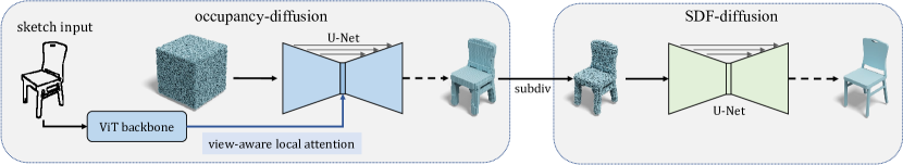
Figure 2. Our LAS-Diffusion model includes two stages: occupancy-diffusion and SDF-diffusion. Occupancy-diffusion takes a noisy $64^{3}$ voxel grid as input, and uses a 3D U-Net to transform the volume to an occupancy volume. The occupied voxels are subdivided into a $128^{3}$ sparse voxel grid and filled with random noise. SDF-diffusion takes this noisy sparse voxel grid as input, and transforms noise signals to SDF values via a 3D sparse-voxel-based U-Net. For sketch-conditional inputs, the local image patch features obtained from a pretrained ViT backbone interact with U-Net voxel features via a view-aware local attention mechanism, to offer local controllability and better generalizability.

Discrete signed distance function

We choose discrete signed distance functions (SDF) as our 3D representation. A discrete signed distance function $g:\mathbf{z}\in\mathcal{Z}\mapsto\mathbb{R}$ is defined on a regular 3D grid $\mathcal{Z}$ or a subset of $\mathcal{Z}$. $g(\mathbf{z})$ records the signed distance from the centers of the grid cells to a closed manifold surface $\mathcal{S}$. Its zero isosurface in polygonal mesh format can be extracted from the dual grid of $\mathcal{Z}$ using the Marching Cube algorithm (Lorensen and Cline, 1987).

Discrete surface-occupancy function

A discrete signed distance function $g$ can be converted into a discrete surface occupancy function $o:\mathbf{z}\in\mathcal{Z}\mapsto\{0,1\}$ as follows: $o(\mathbf{z})=1$ if $|g(\mathbf{z})|\leq\delta$; otherwise, $o(\mathbf{z})=0$. Here, $\delta>0$ is the predefined threshold. The set of $\Omega_{o}:=\{\mathbf{z}\in\mathcal{Z}:o(\mathbf{z})=1\}$ collects the grid cells whose shortest distance from their centers to the surface is no more than $\delta$. Here, note that $\Omega_{o}$ approximates the thin shell of a 3D shape only.

Two-stage diffusion

To represent the details and small features of 3D shapes in discrete SDF format, a high-resolution grid is needed. However, it is not practical to generate a high-resolution and full-grid discrete SDF due to its cubic complexity in memory storage and computational cost. To overcome this issue, we designed a two-stage generation framework based on a self-conditioning continuous diffusion model (Section 3.2): The first stage generates a low-resolution discrete surface-occupancy function to approximate the shell of the shape (Section 3.3), and the second stage focuses on generating fine-grained discrete SDF values inside the occupied region (Section 3.4). We name these two stages by occupancy-diffusion and SDF-diffusion, respectively. In our implementation, the low resolution of the discrete surface-occupancy function is set to $64^{3}$, and the fine resolution of the discrete SDF is $128^{3}$.

Sketch-conditioned generation

To incorporate 2D sketches as guidance, we use the local patch features of the sketch image to assist network learning in a view-aware and cross-attention manner (Section 3.5). This mechanism is called view-aware local attention. Compared to using a global image feature as guidance, view-aware local attention provides better local controllability and makes the model generalizable to unseen sketches.

Fig. 2 illustrates the pipeline of our two-stage diffusion. Each diffusion module is trained individually, and their network architectures are presented in the following subsections.

3.2. Self-conditioning Continuous Diffusion Model

Continuous denoising diffusion

A typical continuous denoising diffusion model (Sohl-Dickstein et al., 2015; Ho et al., 2020; Kingma et al., 2021) consists of the forward process and the reverse process. The forward process introduces a sequence of increasing (Gaussian) noise to a data point $\bm{x}_{0}$, such that it ends up at $\bm{x}_{t}$ that follows the predefined Gaussian distribution. Here, $t$ runs from 0 to 1 in a continuous way. The reverse process maps a noise $\bm{\epsilon}$ sampled from a Gaussian distribution to a data point $\bm{x}_{0}$ through a series of state transitions. The forward process from $\bm{x}_{0}$ to $\bm{x}_{t}$ can be defined as follows.

(1) $$\bm{x}_{t}=\sqrt{\gamma(t)}\bm{x}_{0}+\sqrt{1-\gamma(t)}\bm{\epsilon},$$

where $\bm{\epsilon}\sim\mathcal{N}\left(\bm{0},\bm{I}\right),t\sim\mathcal{U}(0,1)$, and $\gamma(t)$ is a monotonically decreasing function from 1 to 0. $\mathcal{N}$ and $\mathcal{U}$ denote Gaussian distribution and uniform distribution, respectively. In our implementation, we follow (Kingma et al., 2021) to set $\gamma(t)=e^{-10t^{2}-10^{-4}}$.

The prediction from $\bm{x}_{t}$ to $\bm{x}_{0}$ can be modeled by a neural network $f(\bm{x}_{t},t)$. The network training is based on the following denoising loss:

(2) $$\mathcal{L}_{\bm{x}_{0}}=\mathbb{E}_{\bm{\epsilon}\sim\mathcal{N}\left(\bm{0},\bm{I}\right),t\sim\mathcal{U}\left(0,1\right)}\left\|f\left(\bm{x}_{t},t\right)-\bm{x}_{0}\right\|_{2}^{2}.$$

Here, $\bm{x}_{t}$ is sampled via Eq. 1. $f$ is usually implemented as a U-Net architecture. The sampling methods such as DDPM (Ho et al., 2020) and DDIM (Song et al., 2020) strategy can be used for sample generation. For conditioned 3D generation, we adopt the classifier-free guidance (Ho and Salimans, 2021) technique.

Self-conditioning

Recently, Chen et al.  (2023) introduced the self-conditioning mechanism, which uses the previously generated samples as conditioning to significantly improve diffusion models. This mechanism is simple: a neural network $f(\bm{x}_{t},\tilde{\bm{x}}_{0},t)$ is trained to map $\bm{x}_{t}$ to $\bm{x}_{0}$, where $\tilde{\bm{x}}_{0}$ is an estimated $\bm{x}_{0}$ from the previous prediction. The loss function Eq. 2 is revised as follows.

(3) $$\mathcal{L}_{\bm{x}_{0}}=\mathbb{E}_{\bm{\epsilon}\sim\mathcal{N}\left(\bm{0},\bm{I}\right),t\sim\mathcal{U}\left(0,1\right)}\left\|f\left(\bm{x}_{t},\tilde{\bm{x}}_{0},t\right)-\bm{x}_{0}\right\|_{2}^{2}.$$

As suggested by (Chen et al., 2023), during network training, $\tilde{\bm{x}}_{0}$ is set to $f\left(\bm{x}_{t},\bm{0},t\right)$ with probability $p$, and $\bm{0}$ with probability $1-p$, i.e. , without self-conditioning. Here, $p$ is set to $0.5$ by default. Gradient backpropagation on $\tilde{\bm{x}}_{0}$ is disabled to reduce the total training time.

3.3. Occupancy-diffusion Module

Our occupancy-diffusion module is designed to transfer a noisy coarse grid to a discrete surface-occupancy function of a 3D shape. In the following, we introduce the creation of ground-truth discrete surface-occupancy functions and the network architecture.

Data preparation

For each 3D shape in the dataset, we normalize it to fit in a $[-0.8,0.8]^{3}$ box, and compute the discrete SDF function with resolution $128^{3}$ in $[-1,1]^{3}$ using the algorithm of (Xu and Barbič, 2014). This step is similar to (Zheng et al., 2022). Based on the fact that any voxel in a $64^{3}$ grid contains 8 subvoxels of the $128^{3}$ grid. We create a discrete surface-occupancy function $o$ in $64^{3}$ resolution as follows: $o(\mathbf{z})=1$ if there exists a subvoxel of $\mathbf{z}$ whose stored SDF value $v$ satisfies $|v|\leq\frac{1}{32}$; otherwise, $o(\mathbf{z})$ is set to 0.

Network architecture

The U-Net structure in the module is built on the standard 3D convolutional neural network. The U-Net has 5 levels: $64^{3}$, $32^{3}$, $16^{3}$, $8^{3}$, $4^{3}$, and the feature dimensions are $32$, $64$, $128$, $256$, and $256$, respectively. Each level is made up of a ResNet block that contains two convolution layers with kernel size 3. In the bottleneck of U-Net, we add two ResNet blocks. A convolution layer is attached at the end of the network to map the voxel features at the finest level to a surface-occupancy value.

Network training

Eq. 3 is used for network training. More specifically, $\bm{x}_{0}$ is the tensor that stores the ground-truth discrete surface-occupancy values of the grid. As we use the self-conditioning continuous diffusion model, the estimated $\tilde{\bm{x}}_{0}$ is treated as an additional input channel to the U-Net.

Network inference

The $64^{3}$ grid is first initialized with Gaussian noise, then we denoise it in a finite number of steps, using the DDPM sampling strategy (Ho et al., 2020). We reserve the voxels whose predicted surface-occupancy values are larger than $0.5$, and subdivide them once to obtain a set of subvoxels in $128^{3}$ resolution.

3.4. SDF-diffusion Module

For a set of sparse voxels with noisy SDF values, our SDF-diffusion module is designed to map it to the discrete SDF function that represents a real shape. We use the $128^{3}$ discrete SDF functions as described in Section 3.3 for training. The U-Net structure is similar to the one used for occupancy-diffusion except that (1) we use octree-based convolution neural network (Wang et al., 2017, 2020) as the SDF data is stored in sparse voxel format; (2) the U-Net has 4 levels: $128^{3}$, $64^{3}$, $32^{3}$, $16^{3}$, and the feature dimensions are $32,64,128,256$, respectively. The network training is similar to occupancy-diffusion, and $\bm{x}_{0}$ in the loss function corresponds to the SDF values stored at the finest octree nodes.

Network inference

The subdivided voxels from occupancy-diffusion are initialized with Gaussian noise, we denoise it through the DDPM sampling strategy and apply the Marching Cube algorithm (Lorensen and Cline, 1987) on the dual grids of the resulting discrete SDF function to obtain the mesh output.

3.5. View-aware Local Attention

Our approach supports sketch-conditioned shape generation by a novel view-aware local attention mechanism. For a sketch image input, we assume that the view information of the sketch is known, i.e. , camera position and orientation with respect to the shape in a canonical pose. Thus, we can align the image and the 3D grid volume according to the view projection. Inspired by the works of (Wang et al., 2018; Xu et al., 2019) that leverage pixel-level image features for shape reconstruction, we propose to use local image patch features to guide surface-occupancy generation, via feature cross-attention, as follows.

Patch feature extractor

We choose the vision-transformer (ViT) backbone pre-trained on a large volume of images as our sketch image feature extractor. The ViT backbone represents an input image as a series of non-overlapped image patches, denoted by $P_{1},P_{2},\cdots$, and encodes the image into a set of patch-wise features (Dosovitskiy et al., 2021).

\begin{overpic}[width=368.57964pt]{view-projection-0407} \put(80.0,30.0){\small$V$} \put(72.0,40.5){\small$U$} \put(58.0,8.5){\small$\mathbf{p}$} \put(58.0,2.5){\small$\mathcal{N}_{V}$} \put(29.0,40.0){\small$\mathbf{q}$} \put(49.0,39.0){\small$\mathcal{N}_{U}$} \put(31.0,-2.0){\small image plane} \put(75.0,11.5){\small voxel grid} \end{overpic}

Figure 3. Illustration of our view-aware local attention mechanism. For voxel $V$, its voxel center is projected onto the image plane at $\mathbf{p}$, via a known perspective projection. We use the image patch features of the local patches around $\mathbf{p}$ (in yellow color), to interact with voxel feature at $V$ in the U-Net, via cross-attention. For other voxels such as $U$, the operation is similar.

View-aware local attention

We let the voxel features in the U-Net of the occupancy-diffusion module interact with the image patch features according to their view-projection-based relationship. For any voxel $V$ in the grid, we project its center onto the sketch image and obtain the projected coordinate $\mathbf{p}$. Neighboring image patches close to $\mathbf{p}$ are selected to interact with $V$ because their features are highly likely to affect local geometry controlled by $V$. The set of neighborhood image patches is denoted by $\mathcal{N}_{V}$, and selected as follows: patch $P_{j}$ belongs to $\mathcal{N}_{V}$ if the distance between $\mathbf{p}$ and the center of $P_{j}$ is less than a distance threshold $d_{\delta}$. Fig. 3 illustrates the relationship between a voxel and its related image patches.

We use one-layer multi-head cross-attention (Vaswani et al., 2017) to model feature interaction between the voxel feature $f_{V}$ at $V$ and the set of image patch features $f_{I}$ that belongs to the patches in $\mathcal{N}_{V}$, as follows.

(4) $$Q=f_{V}\mathbf{W}^{Q},K=f_{\mathcal{N}}\mathbf{W}^{K},V=f_{\mathcal{N}}\mathbf{W}^{V};$$

$$f_{V}^{\text{new}}=\text{MH-Attention}\left(Q,K,V,\mathcal{M}\right).$$

Here, $\text{MH-Attention}(\cdot)$ is the standard multi-head attention operation, $\mathcal{M}$ is the mask for attention calculation induced by view projection, and we use absolute positional encoding for both voxels and image patches.

Due to the use of patch features, our view-aware local attention is not sensitive to small errors of projection views, as a small view perturbation may still result in similar local patch sets. Therefore, our design is friendly to sketch-conditioned 3D generation, and the user only needs to provide a rough guess of view information, either by a manual way or with the aid of a view prediction network.

Implementation

We use a huge ViT model pre-trained on Laion2B dataset (lai, 2022) as our ViT backbone. Its default input image resolution is $224\times 224$ and the patch_width is $14$. The default value of $d_{\delta}$ is set to $4\times\texttt{patch\_width}$. The weights of the ViT backbone are frozen for our use. To reduce computational cost, only the voxels at $8^{3}$ and $4^{3}$ levels are involved in view-aware local attention. We also experienced using view-aware local attention in our SDF-diffusion module, but found that it has limited improvement to local geometry; thus we introduce view-aware local attention to occupancy-diffusion only.

4. Sketch-conditioned Shape Generation

In this section, we exhibit and validate the capability of LAS-Diffusion for sketch-conditioned shape generation.

4.1. Model Training

Figure 4. Left: Camera setup. Right: Shading images and sketches under the predefined views.

Training dataset

We choose 5 categories from ShapeNetV1 (Chang et al., 2015): chair, car, airplane, table, and rifle for training our sketch-conditioned model.

Predefined perspective views

To make our model convenient to use, we provide five perspective views for user selection and prepare the corresponding sketch data for training. For a normalized shape in its canonical pose, we place five cameras on the scaled bounding sphere of the shape, as shown in Fig. 4-left. These five perspective views are chosen because the sketches under these views are informative and normal users tend to use these view directions or their nearby view directions to draw sketches. The user can pick one of the predefined views that best matches the input sketches for model inference. For convenience, we denote these views by left, side-left, front, side-right, and right. Fig. 4 illustrates shading images and sketches of a chair model under these predefined views.

Data preparation

For each shape in the dataset, we render its shading images from different views and extract their edges via Canny edge detector (Canny, 1986), as 2D sketches. Note that other kinds of sketch synthesis techniques can be used, and we use Canny edge for simplicity. We restrict the rendered views to the predefined views with random perturbation to improve the robustness of the network. The random perturbation is implemented by perturbing the azimuth angle by a noise within $\pm$$$ and the elevation angle by a noise within $\pm$$$. For each predefined view, we perturb $10$ times. In total, there are $50$ sketches for a shape. During training, the corresponding views of these sketches are grouped into their predefined perspective views. To enhance local prior learning, we also augmented shape data by simply uniting two randomly selected shapes for occupancy-diffusion module training, where the shapes are also translated randomly. The number of augmented shapes is the same as the number of original shapes. We trained a single sketch-conditioned LAS-Diffusion model on the five chosen shape categories.

Training details

We trained the occupancy-diffusion module using Adam optimizer (Kingma and Ba, 2014) with a fixed learning rate of $2\times 10^{-4}$ over $300$ epochs. For the training of the SDF-diffusion module, we used AdamW optimizer (Loshchilov and Hutter, 2019) with a fixed learning rate of $10^{-4}$ over $500$ epochs, and its training split follows (Chen and Zhang, 2019).

Inference efficiency

The inference time of our model on a machine with an Nvidia 1080 Ti GPU takes around 10 seconds, using a 50-step DDPM sampling strategy.

Competing methods

We choose the following representative sketch-to-3D methods for comparison: Sketch2Model (Zhang et al., 2021), Sketch2Mesh (Guillard et al., 2021) and SketchSampler (Gao et al., 2022b). Sketch2Model has trained its category-specific models on 13 ShapeNet categories and Sketch2Mesh has trained its category-specific models on car and chair categories. SketchSampler has trained a single model on 13 ShapeNet categories. As SketchSampler is only capable of producing point clouds, we convert them to meshes using SAP (Peng et al., 2021) for quantitative evaluation. For all the above methods, we use their pre-trained models for comparison.

Evaluation metrics

Since there is no previous work designing evaluation metrics for sketch-conditioned probabilistic generative methods, we adapt CLIP score (Hessel et al., 2021) to evaluate perception difference as follows. For a generated 3D shape conditioned on a sketch $I$, we render its sketch $G$ under the same view of the input sketch by our data preparation pipeline, then compute the cosine similarity between the clip features of these two sketches:

(5) $$\text{CLIPScore}(I,G)=100\times\langle E_{I},E_{G}\rangle.$$

Here, $E_{I}$ and $E_{G}$ are the normalized CLIP features of $I$ and $G$, respectively, and $\langle\cdot,\cdot\rangle$ is inner product. The score is averaged over all test data. We also treat the non-white pixels of sketches as 2D points and measure the 2D Chamfer distance between $I$ and $G$, denoted by Sketch-CD. The reconstruction metrics such as CD, EMD, and Voxel-IOU from SketchSampler (Gao et al., 2022b) are also adopted to evaluate the 3D quality of the generated or reconstructed shapes with respect to the shapes that the sketches correspond to.

4.2. Model Evaluation

Table 1. Quantitative evaluations on IKEA chairs. The units of Sketch-CD, CD, EMD and Voxel-IOU are $10^{-4}$, $10^{-3}$, $10^{-2}$ and $10^{-2}$, respectively. SketchSampler_m denotes the version that the point cloud outputs of SketchSampler is converted to polygonal meshes.

Method	CLIPScore$\uparrow$	Sketch-CD$\downarrow$	CD$\downarrow$	EMD$\downarrow$	Voxel-IOU$\uparrow$
Sketch2Model	88.77	101.0	49.38	20.31	22.76
Sketch2Mesh	93.46	37.64	19.16	16.39	32.40
SketchSampler	N/A	N/A	32.51	20.24	33.82
SketchSamplerm	90.43	42.94	33.41	21.24	26.67
LAS-Diffusion	96.92	10.33	06.48	08.85	49.83

Quantitative and qualitative evaluation

We choose IKEA (Lim et al., 2013) chair dataset as the test bed, which contains $35$ chairs. Each chair is rendered from a random view to generate a sketch. For our model, we use one of the predefined views that best matches the input sketch for model inference. We provide accurate view information to Sketch2Model and Sketch2Mesh, and use suggestive (DeCarlo et al., 2003) algorithm to prepare sketches for Sketch2Mesh to match its training style. Compared with other methods, our LAS-Diffusion achieves significantly better performance, as reported in Table 1. Fig. 5 visualizes the results of different methods. The results of LAS-Diffusion are the most plausible and possess better geometry quality. We also render the synthetic sketches of their results in Fig. 6, and find that our results match better with the input sketch. In the supplemental material, we provide all of our generation results.

\begin{overpic}[width=411.93767pt]{images/ikea.pdf} \put(7.0,-3.0){\scriptsize{Sketch2Model}} \put(20.8,-3.0){\scriptsize{Sketch2Mesh}} \put(34.0,-3.0){\scriptsize{SketchSampler}} \put(48.0,-3.0){\scriptsize{LAS-Diffusion}} \put(66.0,-3.0){\scriptsize{GT}} \end{overpic}

Figure 5. Sketch-conditioned shape generation on IKEA chairs.

\begin{overpic}[width=411.93767pt]{images/sketch_compare2.pdf} \put(52.0,0.0){ \leavevmode\hbox to0.4pt{\vbox to97.14pt{\text{[drawing]}}} } \end{overpic}

Figure 6. The sketches of the results shown in Fig. 5. From left to right: Sketch2Model, Sketch2Mesh, SketchSampler, LAS-Diffusion and GT.

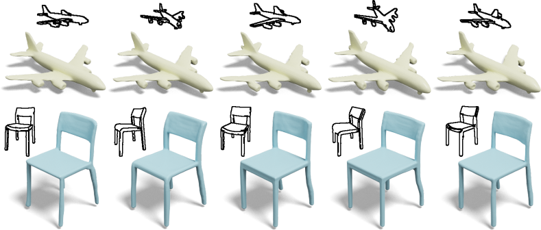
Figure 7. View robustness test. The views for model inference are side-left (top row) and side-right (bottom row).

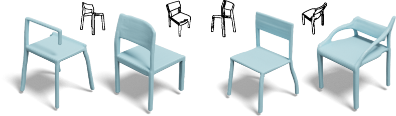
Figure 8. Stress test on view robustness. The view for model inference is side-right.

View robustness

Although only predefined views can be used in our model inference, our model is robust to small view perturbation due to the use of image patch features and random view perturbation during training. In Fig. 7, we illustrate model robustness on two test cases. For each case, we provide 5 different input sketches and we use their most similar view for model inference. We can see that the generated shapes have consistent and good geometry. We also add a stress test in which the input sketches are very different from the predefined side-right view (see Fig. 8), our model is still capable of producing chair-like shapes although some parts are distorted and incomplete due to the use of wrong view information.

\begin{overpic}[width=411.93767pt]{images/add_bars.pdf} \put(4.0,-3.0){\scriptsize{Sketch2Model}} \put(31.0,-3.0){\scriptsize{LAS-Diffusion}} \put(56.0,-3.0){\scriptsize{Sketch2Model}} \put(83.5,-3.0){\scriptsize{LAS-Diffusion}} \put(50.0,0.0){ \leavevmode\hbox to0.4pt{\vbox to114.21pt{\text{[drawing]}}} } \end{overpic}

Figure 9. The six input sketches have different numbers of horizontal bars. LAS-Diffusion has a high probability to generate 3D shapes that match the sketch inputs.

Local controllability

The view-aware local attention mechanism of our LAS-Diffusion model offers nice local controllability, as demonstrated by the example shown in Fig. 9, where a table sketch is modified to have different numbers of horizontal bars. LAS-Diffusion captures local changes well and has a high probability of generating structurally correct and geometry-plausible results. In contrast, the reconstruction-based approach — Sketch2Model (Zhang et al., 2021) cannot handle these structural changes well.

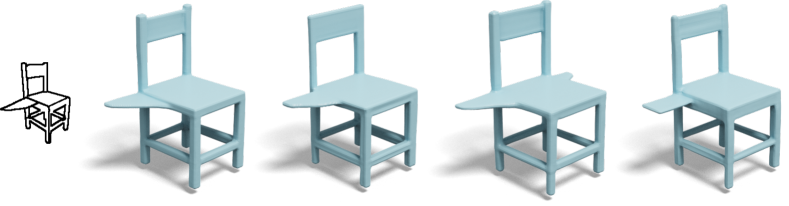
Figure 10. Shape generation conditioned on a creative sketch input.

Model generalizability

We evaluate our model generalizability from the following four aspects.

1. Unseen structural variations. As LAS-Diffusion utilizes local image priors, it is well suited to generate 3D shapes with unseen structural variations. Fig. 10 demonstrates this model generalizability by using a creative sketch input where a chair is attached with a wing-like part. We generate four results using LAS-Diffusion with different noises. The wing part appears in all the results, with some geometry variations. Fig. 11 shows two more examples conditioned by creatively designed sketches. We also tested Sketch2Model, Sketch2Mesh, and SketchSampler on them. Both Sketch2Model and Sketch2Mesh fail to reconstruct the geometry unseen by their training set. SketchSampler has better generalizability due to the use of view-dependent depth sampling, but its predicted depth values do not meet the expectation and the quality of its output point clouds is low.

2. Unseen shape categories. In Fig. 12, we tested sketches of some objects that do not belong to the categories we trained. LAS-Diffusion can generate meaningful results. We attribute its success to local prior learning enabled by our view-aware local attention mechanism, and speculate that the local geometry shown in these examples may exist in the training data.

3. Freehand sketches. Due to our local attention mechanism and the use of the pre-trained ViT image encoder, our model is tolerant of imprecise sketches and varied stroke widths that are different from our rendering setting, thus supporting freehand sketch input. In Fig. 13, we provide some freehand-sketch-conditioned results.

4. Professional sketches. Sketch styles from professional artists are different from our synthetic sketches. We tested the robustness of our model to professional sketches using the ProSketch-3D dataset (Zhong et al., 2020b) which contains $500$ chairs and $1500$ sketches drawn by artists. As the elevation angle of the sketch view of ProSketch-3D data has a $20\mathrm{°}$ difference from our predefined view, we re-trained our model by adjusting the elevation angle of our default views with $20\mathrm{°}$ in our synthetic training data. This new model is denoted by LAS-Diffusion^⋆. Table 2 reports the performance of our method and other competing methods. We can see that LAS-Diffusion^⋆ achieves the best performance. Fig. 14 illustrates our results.

\begin{overpic}[width=411.93767pt]{images/local_control} \put(10.0,-3.0){\scriptsize{Sketch2Model}} \put(30.0,-3.0){\scriptsize{Sketch2Mesh}} \put(56.0,-3.0){\scriptsize{SketchSampler}} \put(85.0,-3.0){\scriptsize{LAS-Diffusion}} \end{overpic}

Figure 11. Comparisons of model generalizability. The results of SketchSampler (Gao et al., 2022b) are rendered from two different views, for better visualization.

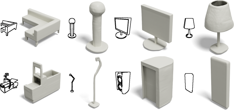
Figure 12. Our LAS-Diffusion model exhibits good generalizability to the sketches beyond the training categories.

Figure 13. Our LAS-Diffusion model is capable of supporting freehand sketches.

Table 2. Quantitative evaluations on the ProSketch dataset. The units of Sketch-CD, CD, EMD and Voxel-IOU are the same as in Table 1.

Method	CLIPScore$\uparrow$	Sketch-CD$\downarrow$	CD$\downarrow$	EMD$\downarrow$	Voxel-IOU$\uparrow$
Sketch2Model	86.52	214.8	105.0	30.10	12.76
Sketch2Mesh	89.84	43.29	21.39	17.13	28.75
SketchSampler	N/A	N/A	58.25	24.04	21.81
SketchSamplerm	89.40	59.88	55.24	24.47	19.64
LAS-Diffusion	93.36	55.62	26.04	16.07	33.43
LAS-Diffusion⋆	93.70	39.75	19.56	14.73	34.97

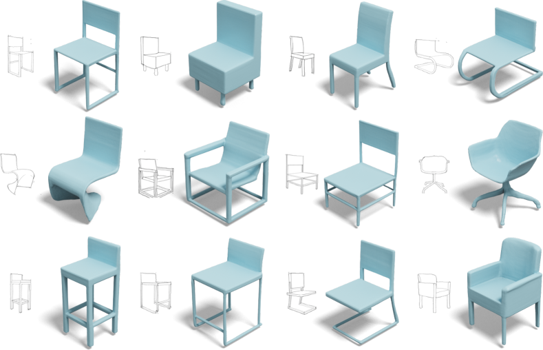
Figure 14. Our model supports sketches drawn by professional artists and generates plausible results. The sketches are from the ProSketch-3D dataset.

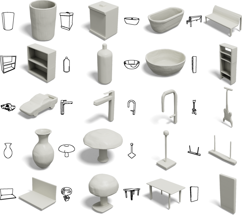
Figure 15. We trained our LAS-Diffusion model on the whole ShapeNetV1 dataset. Some randomly picked results are visualized.

Model scalability

Our LAS-Diffusion model is scalable to more diverse sketch data and random views. We trained a single LAS-Diffusion model on the whole ShapeNetV1 dataset, without restricting views to predefined views. During training, each shape is rendered from random views to generate sketches. Fig. 15 visualizes the sketch-conditioned generative results by this model.

Shape generation via ViT feature manipulation

Our model supports a new way to generate novel shapes by swapping ViT patch features of two existing sketches. For instance, we can replace the top-half patch features of a sketch with the bottom-half features of another sketch, to mimic a shape assembled by the top-half part of the first shape and the bottom-half of another shape. In Fig. 16, we present two novel shapes generated in this way. These interesting results indicate that ViT feature manipulation can be a novel and promising way of controlling shape generation.

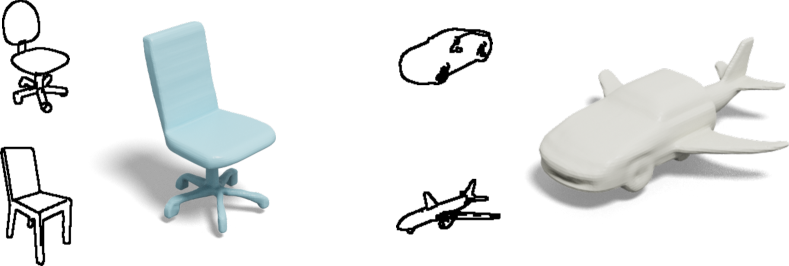
Figure 16. Shape generation via ViT feature manipulation. Left: The bottom half patch features of the swivel chair and the top half patch features of the four-legged chair are stitched together. Right: The left half-patch features of the car and the right half-patch features of the airplane are stitched together. In both cases, novel and meaningful shapes are generated by LAS-Diffusion, without drawing new sketches.

4.3. Ablation Studies

We designed two alternative attention mechanisms to replace our view-aware local attention.

1. Global attention. Instead of using local patch features, we directly use the global image feature to guide voxel feature learning. The global feature is from the classification token of the pre-trained ViT backbone. It is projected via MLP to align with the U-Net feature dimension, and associate with the U-Net feature vectors of the occupancy diffusion module at each level via element-wise multiplication.

2. View-agnostic attention. We let the voxel features in the U-Net of the occupancy-diffusion module interact with all the image patch features via cross-attention, i.e. , the mask $\mathcal{M}$ in Eq. 4 is None. In this way, no view information is required. The involved levels remain unchanged.

We trained LAS-Diffusion using the above attention mechanisms and found that: (1) Global attention has very limited generalizability, and cannot process unseen shape structures; (2) View-agnostic attention responds to sketch variations but often yields additional and wrong geometry, due to loss of local attention. Fig. 17 illustrates these issues.

\begin{overpic}[width=390.25534pt]{images/ablation-update} \put(32.0,-3.0){\scriptsize{global}} \put(56.0,-3.0){\scriptsize{view-agnostic}} \put(87.0,-3.0){\scriptsize{default}} \end{overpic}

Figure 17. Ablation studies on different attention mechanisms. From left to right: global attention, view-agnostic attention, and our default attention — view-aware local attention.

Ablation study on neighborhood size

As seen in the above ablation study, view-agnostic attention does not yield satisfying results, because the attention region is too large and makes feature learning harder. As the local attention plays an important role, we examine how the neighborhood size $d_{\delta}$ affects our model, by varying $d_{\delta}$ from the default $4\times\texttt{patch\_width}$ to $2\times\texttt{patch\_width}$ and $6\times\texttt{patch\_width}$ and retraining our model. We found that the models with these small neighborhood sizes have similar performance. Our default setting has the best CLIP scores on IKEA chairs: 96.63 ($2\times\texttt{patch\_width}$), 96.92 ($4\times\texttt{patch\_width}$), and 96.67 ($6\times\texttt{patch\_width}$).

5. Category-conditioned Shape Generation

In this section, we conducted extensive experiments and evaluations on the task of category-conditioned shape generation.

Dataset

We also use the five shape categories from ShapeNetV1: chair, car, airplane, table, and rifle, to verify the generation capability and quality of LAS-Diffusion without sketch input. We follow the train/val/test split of (Chen and Zhang, 2019).

Training configurations

We have two training configurations, depending on whether a single category is used for training.

1. Single-category generation: we train our model in a single-category manner, i.e. , there are 5 LAS-Diffusion models in total. This per-category model is setup for a fair comparison with other existing 3D shape generative models.

2. Multi-category-conditioned generation: we train a single LAS-Diffusion model on 5 categories to evaluate model scalability. We encode the class name, such as “a chair”, by a pre-trained CLIP network (Radford et al., 2021). We associate the CLIP feature with the U-Net feature vectors of the occupancy diffusion module, as conditions, similar to global attention in Section 4.3. We found empirically that it is not necessary to add CLIP features into the SDF-diffusion stage.

Training details

For both configurations, we trained the occupancy-diffusion module using AdamW optimizer with a fixed learning rate of $10^{-4}$ over $4000$ epochs; and reused the trained SDF-diffusion module from Section 4.

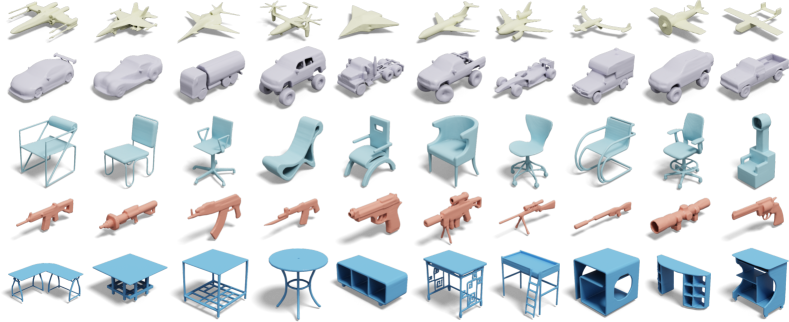
Figure 18. Single-category generation results. Our models were trained on five shape categories: airplane, car, chair, rifle, and table. We selected ten generated shapes from each category to demonstrate shape diversity and high-quality geometry.

Evaluation metric

To evaluate the quality and diversity of generated shapes, we adopt the metric proposed by (Zheng et al., 2022): shading-image-based FID, which avoids the drawback of existing metrics built on light-field-distance (LFD) or 3D mesh distances. To compute this metric, each generated shape was rendered from 20 uniformly distributed views, and its shading images are used to compute FID scores, on the rendered image set of the original training dataset. The metric formula is defined as follows.

(6) $$FID=\frac{1}{20}\left[\sum_{i=1}^{20}\|\mu_{g}^{i}-\mu_{r}^{i}\|^{2}+\operatorname{Tr}\left(\Sigma_{g}^{i}+\Sigma_{r}^{i}-2\left(\Sigma_{r}^{i}\Sigma_{g}^{i}\right)^{1/2}\right)\right],$$

where $g$ and $r$ denote the features of the generated data set and the training set, $\mu^{i}$, $\Sigma^{i}$ denote the mean and covariance matrices of the shading images rendered from the $i$-th view, respectively. A lower FID indicates better generation quality and diversity.

Evaluation and comparisons

Fig. 18 illustrates high-quality and diverse generation results by our single-category LAS-Diffusion model. The results show that our model can generate structurally complex shapes with fine geometry. More uncurated generated results including intermediate occupancy generation are provided in the supplemental material.

We compared our approach with four representative 3D generation models, including two GAN-based models: IM-GAN (Chen and Zhang, 2019) and SDF-StyleGAN (Zheng et al., 2022), a 3D diffusion model: Wavelet-Diffusion (Hui et al., 2022) and an autoregressive model: 3DILG (Zhang et al., 2022). We use their pre-trained models for evaluation. Except for 3DILG which was trained on all ShapeNetV2 data and our multi-category-conditioned model, other methods were trained on a single category. Here, IM-GAN and Wavelet-Diffusion use $256^{3}$ occupancy and SDF fields as ground truth for training, respectively.

Table 3. Quantitative comparison with different methods. The reported numbers are shading-image-based FID scores (lower is better). LAS-Diffusion^† and LAS-Diffusion^‡ denote the single-category models and multi-category-conditioned model, respectively. Note that Wavelet-Diffusion was trained on 3 categories only.

Method	Chair	Airplane	Car	Table	Rifle
IM-GAN	63.42	74.57	141.2	51.70	103.3
SDF-StyleGAN	36.48	65.77	97.99	39.03	64.86
Wavelet-Diffusion	28.64	35.05	N/A	30.27	N/A
LAS-Diffusion†	20.45	32.71	80.55	17.25	44.93
3DILG	31.64	54.38	164.15	54.13	77.74
LAS-Diffusion‡	21.55	43.08	86.34	17.41	70.39

Table 3 reports the FID scores of all methods. We conclude that: (1) our single-category LAS-Diffusion outperforms other methods in all five categories; (2) our multi-category-conditioned LAS-Diffusion is slightly worse than its unconditioned version, but still performs better than other methods, except for airplane (Wavelet-Diffusion) and rifle (SDF-StyleGAN). The comparison with 3DILG is for reference only, as their training data are not exactly the same. In Fig. 19, we visualize some chairs generated by different methods. We can see that Wavelet-Diffusion, 3DILG, and our LAS-Diffusion are visually comparable and possess a more faithful geometry than IM-GAN and SDF-StyleGAN, furthermore, the meshes generated by our method have less bumpy geometry than others.

\begin{overpic}[width=411.93767pt]{images/visual_compare.pdf} \put(5.0,-3.0){\scriptsize{IM-GAN}} \put(18.5,-3.0){\scriptsize{SDF-StyleGAN}} \put(35.0,-3.0){\scriptsize{Wavelet-Diffusion} } \put(59.0,-3.0){\scriptsize{3DILG}} \put(72.5,-3.0){\scriptsize{LAS-Diffusion}} \end{overpic}

Figure 19. Randomly selected chairs generated by different methods.

Following (Hui et al., 2022), we also adopt the COV, MMD, and 1-NNA metrics (Achlioptas et al., 2018; Yang et al., 2019) based on the Chamfer distance (CD) and the Earth mover’s distance (EMD) on the sampled points to access the fidelity, coverage, and diversity of generative models. Lower MMD, higher COV, 1-NNA that has a smaller difference to $50\text{\,}\mathrm{\char 37\relax}$, mean better quality. We report these metrics in the chair category in Table 4 for IM-GAN, SDF-StyleGAN, Wavelet-Diffusion, and our single-category model. 2048 points were sampled on each mesh uniformly to perform the evaluation. Wavelet-Diffusion and our method are comparable on MMD and 1-NNA, and our method attains better COV(EMD) than other methods.

Table 4. Additional metric evaluations on chair category. The units of CD and EMD are $10^{-3}$ and $10^{-2}$, respectively. LAS-Diffusion^† denotes the single-category model.

Method	c		c		c
	CD	EMD	CD	EMD	CD	EMD
IM-GAN	57.30	49.48	13.12	17.70	62.24	69.32
SDF-StyleGAN	52.36	48.89	14.97	18.10	65.38	69.06
Wavelet-Diffusion	52.88	47.64	13.37	17.33	61.14	66.92
LAS-Diffusion†	53.76	52.43	13.79	17.45	64.53	65.15

\begin{overpic}[width=325.215pt]{images/hist} \put(100.0,8.0){\scriptsize CD} \end{overpic}

\begin{overpic}[width=346.89731pt]{images/retrieval.pdf} \put(22.0,0.0){ \leavevmode\hbox to0.4pt{\vbox to53.61pt{\text{[drawing]}}} } \end{overpic}

Figure 20. Top: The histogram on the distribution of the Chamfer distance (CD) between the generated chairs and the training dataset. Here, we use SquareRoot binning for histogram drawing. Bottom: The four nearest shapes (right) retrieved from the training dataset according to their Chamfer distance to the generated chair (left).

Shape diversity

We also evaluate the model diversity of our method on chair category, by computing the histogram of Chamfer distance between the generated shapes and the training data. Fig. 20-top shows the histogram whose x-axis is Chamfer distance ($\times 10^{3}$). The histogram reveals that most generated shapes are different from the training set. Fig. 20-bottom presents a test case: for the generated chair (left), we retrieve the four most similar chairs (right) from the training dataset based on the Chamfer distance. We can see that the generated chair has a novel structure.

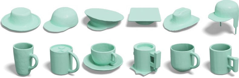
Figure 21. Generation results on small datasets. Top: generated results on cap category. Bottom: generated results on mug category.

Small datasets

We also tested the capability of our single-category LAS-Diffusion on ShapeNet categories that have a small number of objects. We chose cap category (56 objects) as well as mug category (214 objects) to train the occupancy-diffusion module and reused the trained SDF-diffusion module. Fig. 21 shows that the shapes generated by LAS-Diffusion are plausible with good quality.

6. Conclusion and Perspectives

We present a diffusion-based generative technique to synthesize plausible 3D shapes. Our view-aware local attention mechanism is well integrated with our two-stage diffusion model and offers greater controllability and generalizability than existing shape synthesis techniques. As this mechanism is simple and flexible, there is no difficulty in extending it to color images, depth images, and even 3D point cloud inputs. We believe that it will be a powerful module for multimodal-conditioned content generation.

Limitations

Currently, our model is trained on synthetic data only. The sketch style is tied to our rendering pipeline; therefore, our trained model is not well adapted for sketches with highly distorted lines, oversketches, or seriously inconsistent perspectives. An example is shown in the right inset, in which our model fails to generate the chair arm structure for the input with oversketches. We believe that this issue can be overcome by using more real sketches and paired 3D shapes for training.

In the future, we would like to explore the following directions.

Shape appearance

Currently our work focuses on shape geometry only and does not provide vivid shape appearances. As 2D sketches do not contain rich appearance information, we plan to leverage both 2D sketches and language descriptions to generate geometry-compatible and plausible shape appearances.

Multi-view sketches

Single-view sketches do not convey the complete idea of designers. We will study how to utilize multi-view sketches in our model and provide a convenient user interface to assist 3D design.

References

- (1)
- lai (2022) 2022. LAION2B dataset. https://huggingface.co/datasets/laion/laion2B-en.
- Achlioptas et al. (2018) Panos Achlioptas, Olga Diamanti, Ioannis Mitliagkas, and Leonidas Guibas. 2018. Learning representations and generative models for 3D point clouds. In ICML. PMLR, 40–49.
- Alex et al. (2022) Nichol Alex, Jun Heewoo, Dhariwal Prafulla, Mishkin Pamela, and Chen Mark. 2022. Point-E: A system for generating 3D point clouds from complex prompts. arXiv:2212.08751.
- Cai et al. (2020) Ruojin Cai, Guandao Yang, Hadar Averbuch-Elor, Zekun Hao, Serge Belongie, Noah Snavely, and Bharath Hariharan. 2020. Learning gradient fields for shape generation. In ECCV. Springer, 364–381.
- Canny (1986) John Canny. 1986. A computational approach to edge detection. IEEE Trans. Pattern Anal. Mach. Intell. 8 (1986), 679–698. Issue 6.
- Chan et al. (2022) Eric R Chan, Connor Z Lin, Matthew A Chan, Koki Nagano, Boxiao Pan, Shalini De Mello, Orazio Gallo, Leonidas J Guibas, Jonathan Tremblay, Sameh Khamis, et al. 2022. Efficient geometry-aware 3D generative adversarial networks. In CVPR. 16123–16133.
- Chan et al. (2021) Eric R Chan, Marco Monteiro, Petr Kellnhofer, Jiajun Wu, and Gordon Wetzstein. 2021. pi-GAN: Periodic implicit generative adversarial networks for 3d-aware image synthesis. In CVPR. 5799–5809.
- Chang et al. (2015) Angel X Chang, Thomas Funkhouser, Leonidas Guibas, Pat Hanrahan, Qixing Huang, Zimo Li, Silvio Savarese, Manolis Savva, Shuran Song, Hao Su, et al. 2015. ShapeNet: An information-rich 3D model repository. arXiv:1512.03012.
- Chen et al. (2018) Kevin Chen, Christopher B Choy, Manolis Savva, Angel X Chang, Thomas Funkhouser, and Silvio Savarese. 2018. Text2shape: Generating shapes from natural language by learning joint embeddings. In ACCV. 100–116.
- Chen et al. (2023) Ting Chen, Ruixiang Zhang, and Geoffrey Hinton. 2023. Analog Bits: Generating discrete data using diffusion models with self-conditioning. In ICLR.
- Chen et al. (2021) Zhiqin Chen, Vladimir G Kim, Matthew Fisher, Noam Aigerman, Hao Zhang, and Siddhartha Chaudhuri. 2021. DECOR-GAN: 3D shape detailization by conditional refinement. In CVPR. 15740–15749.
- Chen and Zhang (2019) Zhiqin Chen and Hao Zhang. 2019. Learning implicit fields for generative shape modeling. In CVPR. 5939–5948.
- Cheng et al. (2023) Yen-Chi Cheng, Hsin-Ying Lee, Sergey Tulyakov, Alexander Schwing, and Liangyan Gui. 2023. SDFusion: Multimodal 3D shape completion, reconstruction, and generation. In CVPR.
- Cheng et al. (2022) Zezhou Cheng, Menglei Chai, Jian Ren, Hsin-Ying Lee, Kyle Olszewski, Zeng Huang, Subhransu Maji, and Sergey Tulyakov. 2022. Cross-modal 3D shape generation and manipulation. In ECCV. Springer, 303–321.
- Chou et al. (2022) Gene Chou, Yuval Bahat, and Felix Heide. 2022. DiffusionSDF: Conditional generative modeling of signed distance functions. arXiv:2211.13757.
- DeCarlo et al. (2003) Doug DeCarlo, Adam Finkelstein, Szymon Rusinkiewicz, and Anthony Santella. 2003. Suggestive contours for conveying shape. In SIGGRAPH. 848–855.
- Deng et al. (2022) Yu Deng, Jiaolong Yang, Jianfeng Xiang, and Xin Tong. 2022. GRAM: Generative Radiance Manifolds for 3D-Aware Image Generation. In CVPR.
- Dhariwal and Nichol (2021) Prafulla Dhariwal and Alexander Nichol. 2021. Diffusion models beat GANs on image synthesis. NeurIPS 34, 8780–8794.
- Dosovitskiy et al. (2021) Alexey Dosovitskiy, Lucas Beyer, Alexander Kolesnikov, Dirk Weissenborn, Xiaohua Zhai, Thomas Unterthiner, Mostafa Dehghani, Matthias Minderer, Georg Heigold, Sylvain Gelly, et al. 2021. An image is worth 16x16 words: Transformers for image recognition at scale. In ICLR.
- Eitz et al. (2012) Mathias Eitz, James Hays, and Marc Alexa. 2012. How do humans sketch objects? ACM Trans. Graph. 31, 4 (2012), 1–10.
- Fan et al. (2017) H Fan, H Su, and LJ Guibas. 2017. A point set generation network for 3D object reconstruction from a single image. In CVPR.
- Fu et al. (2022) Rao Fu, Xiao Zhan, Yiwen Chen, Daniel Ritchie, and Srinath Sridhar. 2022. ShapeCrafter: A recursive text-conditioned 3D shape generation model. In NeurIPS.
- Gao et al. (2022b) Chenjian Gao, Qian Yu, Lu Sheng, Yi-Zhe Song, and Dong Xu. 2022b. SketchSampler: Sketch-based 3D reconstruction via view-dependent depth sampling. In ECCV. 464–479.
- Gao et al. (2022a) Jun Gao, Tianchang Shen, Zian Wang, Wenzheng Chen, Kangxue Yin, Daiqing Li, Or Litany, Zan Gojcic, and Sanja Fidler. 2022a. Get3D: A generative model of high quality 3D textured shapes learned from images. In NeurIPS.
- Goodfellow et al. (2014) Ian Goodfellow, Jean Pouget-Abadie, Mehdi Mirza, Bing Xu, David Warde-Farley, Sherjil Ozair, Aaron Courville, and Yoshua Bengio. 2014. Generative adversarial nets. In NeurIPS, Vol. 27.
- Guillard et al. (2021) Benoit Guillard, Edoardo Remelli, Pierre Yvernay, and Pascal Fua. 2021. Sketch2Mesh: Reconstructing and editing 3D shapes from sketches. In ICCV. 13023–13032.
- Hessel et al. (2021) Jack Hessel, Ari Holtzman, Maxwell Forbes, Ronan Le Bras, and Yejin Choi. 2021. ClipScore: A reference-free evaluation metric for image captioning. In EMNLP.
- Ho et al. (2020) Jonathan Ho, Ajay Jain, and Pieter Abbeel. 2020. Denoising diffusion probabilistic models. NeurIPS 33, 6840–6851.
- Ho and Salimans (2021) Jonathan Ho and Tim Salimans. 2021. Classifier-free diffusion guidance. In NeurIPS Workshop.
- Hong et al. (2022) Fangzhou Hong, Mingyuan Zhang, Liang Pan, Zhongang Cai, Lei Yang, and Ziwei Liu. 2022. AvatarCLIP: Zero-shot text-driven generation and animation of 3D avatars. ACM Trans. Graph. 41, 4 (2022).
- Hui et al. (2022) Ka-Hei Hui, Ruihui Li, Jingyu Hu, and Chi-Wing Fu. 2022. Neural wavelet-domain diffusion for 3D shape generation. In SIGGRAPHAsia Conference Papers.
- Hui et al. (2020) Le Hui, Rui Xu, Jin Xie, Jianjun Qian, and Jian Yang. 2020. Progressive point cloud deconvolution generation network. In ECCV. Springer, 397–413.
- Ibing et al. (2021a) Moritz Ibing, Gregor Kobsik, and Leif Kobbelt. 2021a. Octree Transformer: Autoregressive 3D shape generation on hierarchically structured sequences. arXiv:2111.12480.
- Ibing et al. (2021b) Moritz Ibing, Isaak Lim, and Leif Kobbelt. 2021b. 3D shape generation with grid-based implicit functions. In CVPR. 13559–13568.
- Jain et al. (2022) Ajay Jain, Ben Mildenhall, Jonathan T Barron, Pieter Abbeel, and Ben Poole. 2022. Zero-shot text-guided object generation with dream fields. In CVPR. 867–876.
- Jiang et al. (2017) Chiyu Jiang, Philip Marcus, et al. 2017. Hierarchical detail enhancing mesh-based shape generation with 3D generative adversarial network. arXiv:1709.07581.
- Khalid et al. (2022) Nasir Khalid, Tianhao Xie, Eugene Belilovsky, and Tiberiu Popa. 2022. Text to mesh without 3D supervision using limit subdivision. In Siggraph Asia Conference Papers.
- Kingma et al. (2021) Diederik Kingma, Tim Salimans, Ben Poole, and Jonathan Ho. 2021. Variational diffusion models. NeurIPS 34, 21696–21707.
- Kingma and Ba (2014) Diederik P Kingma and Jimmy Ba. 2014. Adam: A method for stochastic optimization. arXiv:1412.6980.
- Kleineberg et al. (2020) Marian Kleineberg, Matthias Fey, and Frank Weichert. 2020. Adversarial generation of continuous implicit shape representations. In Eurographics 2020 - Short Papers. The Eurographics Association.
- Kong et al. (2022) Di Kong, Qiang Wang, and Yonggang Qi. 2022. A diffusion-refinement model for sketch-to-point modeling. In ACCV. 1522–1538.
- Li et al. (2018) Changjian Li, Hao Pan, Yang Liu, Xin Tong, Alla Sheffer, and Wenping Wang. 2018. Robust flow-guided neural prediction for sketch-based freeform surface modeling. ACM Trans. Graph. 37, 6 (2018).
- Li et al. (2023) Muheng Li, Yueqi Duan, Jie Zhou, and Jiwen Lu. 2023. Diffusion-SDF: Text-to-shape via voxelized diffusion. In CVPR.
- Lim et al. (2013) Joseph J. Lim, Hamed Pirsiavash, and Antonio Torralba. 2013. Parsing IKEA objects: Fine pose estimation. In ICCV.
- Lin et al. (2023) Chen-Hsuan Lin, Jun Gao, Luming Tang, Towaki Takikawa, Xiaohui Zeng, Xun Huang, Karsten Kreis, Sanja Fidler, Ming-Yu Liu, and Tsung-Yi Lin. 2023. Magic3D: High-resolution text-to-3D content creation. In CVPR.
- Liu et al. (2019) Shichen Liu, Tianye Li, Weikai Chen, and Hao Li. 2019. Soft Rasterizer: A differentiable renderer for image-based 3D reasoning. In ICCV. 7708–7717.
- Liu et al. (2023) Zhengzhe Liu, Peng Dai, Ruihui Li, Xiaojuan Qi, and Chi-Wing Fu. 2023. ISS: Image as stetting stone for text-guided 3D shape generation. In ICLR.
- Lorensen and Cline (1987) William E Lorensen and Harvey E Cline. 1987. Marching cubes: A high resolution 3D surface construction algorithm. SIGGRAPH, 163–169.
- Loshchilov and Hutter (2019) Ilya Loshchilov and Frank Hutter. 2019. Decoupled Weight Decay Regularization. In ICLR.
- Lun et al. (2017) Zhaoliang Lun, Matheus Gadelha, Evangelos Kalogerakis, Subhransu Maji, and Rui Wang. 2017. 3D shape reconstruction from sketches via multi-view convolutional networks. In 3DV. IEEE, 67–77.
- Luo and Hu (2021) Shitong Luo and Wei Hu. 2021. Diffusion probabilistic models for 3D point cloud generation. In CVPR. 2837–2845.
- Lyu et al. (2021) Zhaoyang Lyu, Zhifeng Kong, Xudong Xu, Liang Pan, and Dahua Lin. 2021. A conditional point diffusion-refinement paradigm for 3D point cloud completion. In ICLR.
- Mescheder et al. (2019) Lars Mescheder, Michael Oechsle, Michael Niemeyer, Sebastian Nowozin, and Andreas Geiger. 2019. Occupancy Networks: Learning 3D reconstruction in function space. In CVPR. 4460–4470.
- Michel et al. (2022) Oscar Michel, Roi Bar-On, Richard Liu, Sagie Benaim, and Rana Hanocka. 2022. Text2mesh: Text-driven neural stylization for meshes. In CVPR. 13492–13502.
- Mittal et al. (2022) Paritosh Mittal, Yen-Chi Cheng, Maneesh Singh, and Shubham Tulsiani. 2022. AutoSDF: Shape priors for 3D completion, reconstruction and generation. In CVPR.
- Nam et al. (2022) Gimin Nam, Mariem Khlifi, Andrew Rodriguez, Alberto Tono, Linqi Zhou, and Paul Guerrero. 2022. 3D-LDM: Neural implicit 3D shape generation with latent diffusion models. arXiv:2212.00842.
- Nash et al. (2020) Charlie Nash, Yaroslav Ganin, SM Ali Eslami, and Peter Battaglia. 2020. PolyGen: An autoregressive generative model of 3D meshes. In ICML. PMLR, 7220–7229.
- Niemeyer and Geiger (2021) Michael Niemeyer and Andreas Geiger. 2021. GIRAFFE: Representing scenes as compositional generative neural feature fields. In CVPR. 11453–11464.
- Olsen et al. (2009) Luke Olsen, Faramarz F Samavati, Mario Costa Sousa, and Joaquim A Jorge. 2009. Sketch-based modeling: A survey. Computers & Graphics 33, 1 (2009), 85–103.
- Or-El et al. (2022) Roy Or-El, Xuan Luo, Mengyi Shan, Eli Shechtman, Jeong Joon Park, and Ira Kemelmacher-Shlizerman. 2022. StyleSDF: High-resolution 3D-consistent image and geometry generation. In CVPR. 13503–13513.
- Peng et al. (2021) Songyou Peng, Chiyu Jiang, Yiyi Liao, Michael Niemeyer, Marc Pollefeys, and Andreas Geiger. 2021. Shape as Points: A differentiable poisson solver. NeurIPS 34, 13032–13044.
- Poole et al. (2023) Ben Poole, Ajay Jain, Jonathan T. Barron, and Ben Mildenhall. 2023. DreamFusion: Text-to-3D using 2D diffusion. In ICLR.
- Radford et al. (2021) Alec Radford, Jong Wook Kim, Chris Hallacy, Aditya Ramesh, Gabriel Goh, Sandhini Agarwal, Girish Sastry, Amanda Askell, Pamela Mishkin, Jack Clark, et al. 2021. Learning transferable visual models from natural language supervision. In ICML. 8748–8763.
- Rezende and Mohamed (2015) Danilo Rezende and Shakir Mohamed. 2015. Variational inference with normalizing flows. In ICML. PMLR, 1530–1538.
- Saito et al. (2019) Shunsuke Saito, Zeng Huang, Ryota Natsume, Shigeo Morishima, Angjoo Kanazawa, and Hao Li. 2019. PIFu: Pixel-aligned implicit function for high-resolution clothed human digitization. In ICCV. 2304–2314.
- Sanghi et al. (2022a) Aditya Sanghi, Hang Chu, Joseph G. Lambourne, Ye Wang, Chin-Yi Cheng, Marco Fumero, and Kamal Rahimi Malekshan. 2022a. CLIP-Forge: Towards zero-shot text-to-shape generation. In CVPR. 18603–18613.
- Sanghi et al. (2022b) Aditya Sanghi, Rao Fu, Vivian Liu, Karl Willis, Hooman Shayani, Amir Hosein Khasahmadi, Srinath Sridhar, and Daniel Ritchie. 2022b. TextCraft: Zero-Shot generation of high-fidelity and diverse shapes from text. arXiv:2211.01427.
- Schwarz et al. (2020) Katja Schwarz, Yiyi Liao, Michael Niemeyer, and Andreas Geiger. 2020. GRAF: Generative radiance fields for 3D-aware image synthesis. NeurIPS 33, 20154–20166.
- Shue et al. (2022) J Ryan Shue, Eric Ryan Chan, Ryan Po, Zachary Ankner, Jiajun Wu, and Gordon Wetzstein. 2022. 3D Neural Field Generation using Triplane Diffusion. arXiv:2211.16677.
- Sohl-Dickstein et al. (2015) Jascha Sohl-Dickstein, Eric Weiss, Niru Maheswaranathan, and Surya Ganguli. 2015. Deep unsupervised learning using nonequilibrium thermodynamics. In ICML. 2256–2265.
- Song et al. (2020) Jiaming Song, Chenlin Meng, and Stefano Ermon. 2020. Denoising diffusion implicit models. In ICLR.
- Van Den Oord et al. (2017) Aaron Van Den Oord, Oriol Vinyals, and Koray Kavukcuoglu. 2017. Neural discrete representation learning. NeurIPS 30.
- Van Oord et al. (2016) Aaron Van Oord, Nal Kalchbrenner, and Koray Kavukcuoglu. 2016. Pixel recurrent neural networks. In ICML. 1747–1756.
- Vaswani et al. (2017) Ashish Vaswani, Noam Shazeer, Niki Parmar, Jakob Uszkoreit, Llion Jones, Aidan N Gomez, Łukasz Kaiser, and Illia Polosukhin. 2017. Attention is all you need. NeurIPS 30.
- Wang et al. (2021) Dan Wang, Xinrui Cui, Xun Chen, Zhengxia Zou, Tianyang Shi, Septimiu Salcudean, Z Jane Wang, and Rabab Ward. 2021. Multi-view 3D reconstruction with transformers. In ICCV. 5722–5731.
- Wang et al. (2018) Nanyang Wang, Yinda Zhang, Zhuwen Li, Yanwei Fu, Wei Liu, and Yu-Gang Jiang. 2018. Pixel2Mesh: Generating 3D mesh models from single RGB images. In ECCV. 52–67.
- Wang et al. (2017) Pengshuai Wang, Yang Liu, Yuxiao Guo, Chunyu Sun, and Xin Tong. 2017. O-CNN: Octree-based convolutional neural networks for 3D shape analysis. ACM Trans. Graph. 36, 4 (2017).
- Wang et al. (2020) Peng-Shuai Wang, Yang Liu, and Xin Tong. 2020. Deep Octree-based CNNs with output-guided skip connections for 3D shape and scene completion. In CVPR Workshop.
- Wu et al. (2016) Jiajun Wu, Chengkai Zhang, Tianfan Xue, William T Freeman, and Joshua B Tenenbaum. 2016. Learning a probabilistic latent space of object shapes via 3D generative-adversarial modeling. In NeurIPS. 82–90.
- Xiang et al. (2020) Nan Xiang, Ruibin Wang, Tao Jiang, Li Wang, Yanran Li, Xiaosong Yang, and Jianjun Zhang. 2020. Sketch-based modeling with a differentiable renderer. Computer Animation and Virtual Worlds 31, 4-5 (2020), e1939.
- Xu and Barbič (2014) Hongyi Xu and Jernej Barbič. 2014. Signed distance fields for polygon soup meshes. In Graphics Interface. 35–41.
- Xu et al. (2019) Qiangeng Xu, Weiyue Wang, Duygu Ceylan, Radomir Mech, and Ulrich Neumann. 2019. DISN: Deep implicit surface network for high-quality single-view 3D reconstruction. NeurIPS 32.
- Yan et al. (2022) Xingguang Yan, Liqiang Lin, Niloy J Mitra, Dani Lischinski, Daniel Cohen-Or, and Hui Huang. 2022. Shapeformer: Transformer-based shape completion via sparse representation. In CVPR. 6239–6249.
- Yang et al. (2019) Guandao Yang, Xun Huang, Zekun Hao, Ming-Yu Liu, Serge Belongie, and Bharath Hariharan. 2019. PointFlow: 3D point cloud generation with continuous normalizing flows. In ICCV. 4541–4550.
- Zeng et al. (2022) Xiaohui Zeng, Arash Vahdat, Francis Williams, Zan Gojcic, Or Litany, Sanja Fidler, and Karsten Kreis. 2022. LION: Latent point diffusion models for 3D shape generation. In NeurIPS.
- Zhang et al. (2022) Biao Zhang, Matthias Nießner, and Peter Wonka. 2022. 3DILG: Irregular Latent grids for 3D generative modeling. In NeurIPS.
- Zhang et al. (2021) Song-Hai Zhang, Yuan-Chen Guo, and Qing-Wen Gu. 2021. Sketch2Model: View-aware 3D modeling from single free-hand sketches. In CVPR. 6012–6021.
- Zheng et al. (2022) Xinyang Zheng, Yang Liu, Pengshuai Wang, and Xin Tong. 2022. SDF-StyleGAN: Implicit SDF-based StyleGAN for 3D shape generation. In Comput. Graph. Forum, Vol. 41. 52–63.
- Zhong et al. (2020a) Yue Zhong, Yulia Gryaditskaya, Honggang Zhang, and Yi-Zhe Song. 2020a. Deep sketch-based modeling: Tips and tricks. In 3DV. 543–552.
- Zhong et al. (2022) Yue Zhong, Yulia Gryaditskaya, Honggang Zhang, and Yi-Zhe Song. 2022. A study of deep single sketch-based modeling: View/style invariance, sparsity and latent space disentanglement. Computers & Graphics 106 (2022), 237–247.
- Zhong et al. (2020b) Yue Zhong, Yonggang Qi, Yulia Gryaditskaya, Honggang Zhang, and Yi-Zhe Song. 2020b. Towards practical sketch-based 3D shape generation: The role of professional sketches. IEEE Transactions on Circuits and Systems for Video Technology 31, 9 (2020), 3518–3528.
- Zhou et al. (2021) Linqi Zhou, Yilun Du, and Jiajun Wu. 2021. 3D shape generation and completion through point-voxel diffusion. In ICCV. 5826–5835.