Neural Steerer: Novel Steering Vector Synthesis
with a Causal Neural Field over Frequency and Source Positions

Abstract

Neural fields have successfully been used in many research fields for their native ability to estimate a continuous function from a finite number of observations. In audio processing, this technique has been applied to acoustic and head-related transfer function interpolation. However, most of the existing methods estimate the real-valued magnitude function over a predefined discrete set of frequencies. In this study, we propose a novel approach for steering vector interpolation that regards frequencies as continuous input variables. Moreover, we propose a novel unsupervised regularization term enforcing the estimated filters to be causal. The experiment using real steering vectors show that the proposed frequency resolution-free method outperformed the existing methods operating over discrete set of frequencies.

Keywords Steering vector  $\cdot$ neural field  $\cdot$ spatial audio  $\cdot$ interpolation  $\cdot$ representation learning

1 Introduction

In audio processing, steering vectors describe the spatial relationship between a sound source and a set of sensors used to capture it. They are core components of spatial audio processing systems with applications ranging from immersive audio rendering to automatic speech recognition front end, such as speech enhancement [1], source separation [2], source localization [3], and acoustic channel estimation [4]. Therefore, their correct characterization is fundamental to enable accurate sound analysis and to achieve immersion and realism in rendering.

Algebraic steering vectors analytically encode the direct propagation of an acoustic transfer function or an impulse response over space and frequency or time, respectively. However, for in-the-wild scenarios, their algebraic model is limited by several impairments, and often replace with more general filters [5]. Extended formulations include models for microphone directivity and filtering as well as sound interaction with the receiver, such as occlusion, diffraction, and scattering. In hearing aids application, the steering vectors, also known as head-related transfer function (HRTF), model the filtering effects of the user’s pinnae, head, and torso.

In order to model all the effects at each space and frequency, one can use dedicated acoustics simulators, which suffer from significant realism-computational and modeling complexity trade-offs. Alternatively, steering vectors can be accurately measured in dedicated facilities [1]. Alas, measuring them at high spatial resolution is a cumbersome, time-consuming task, if not unfeasible and prohibitive due to the cost and setup complexity.

Reliable data-driven interpolation approaches have received significant attention over the last decades. These methods use steering vectors measured on a coarse spatial grid as a basis and then interpolate to estimate them at new locations, typically on a finer grid[6]. However, such methods suffer from two main drawbacks. First, they assume that the target quantity undergoes a polynomial transformation of some basis function at the desired spatial location, which may not accurately represent reality and may introduce artifacts. Second, all these methods operate interpolation only in the spatial domain, leaving the frequency (or temporal) grid resolution fixed and limiting the portability of the estimated steering vectors.

Recent deep learning approaches showed that coordinate-based architecture are able to parameterize physical properties of signals continuously over space and time. These methods, called Neural Fields [7], can be trained easily using data-fit and model-based loss function in order to interpolate a target quantity (e.g. image, audio, 3D shape, physical fields) at arbitrary resolution.

In this work, we address the limitation of steering vector interpolation by leveraging recent advances in neural fields. The proposed method models both the magnitude and the phase of steering vectors (and/or HRTFs) as a complex field defined continuously over space and frequency. Based on the theoretical foundation of signal processing, we propose novel regularizers that enforce the estimated filter to be causal, reducing artifacts, leading to more accurate filters. We show that the proposed approach is able to outperform baseline methods in interpolating steering vectors.

2 Related Works

Given a set of steering vector measurements in the time or frequency domain, a simple way to increase the spatial resolution is to obtain an estimate for a new position by weighting known measurements from multiple surrounding positions. Methods of this form are extensions of polynomial interpolation where data are projected onto ad-hoc basis functions (e.g., spherical harmonics or spatial characteristic function) whose coefficients are then interpolated at desired positions [6, 8]. The limitations of these approaches are the requirement of near-uniform sampling for the training data and the performances related to the choice of the basis function and their interpolating methods.

Neural fields (NFs) are coordinate-based neural networks that have been recently proposed to encode or resolve continuous functions estimated from measurements observed either on a discrete grid or random locations. Their outstanding applications include 3D shape reconstruction from sparse 2D images [9], image super-resolution [10], compression [11], and animation of human bodies [12]. Unlike on-grid discrete measurements at a given resolution, the memory complexity for these continuous models scales with the data complexity and not with the desired resolution. In addition, being over-parameterized, adaptive, and modular neural network models, NFs are effective for regressing ill-posed problems under appropriate regularization. However, in practice, they tend to overfit, and their resolution capabilities are limited by network capacity and training data resolution [7].

Interestingly, physics-informed neural networks (PINNs) [13, 14] are similar coordinate-based models proposed in computational physics. Here, the data-fit loss terms are evaluated together with physical models, e.g., partial differential equations, evaluated at arbitrary resolution. The resulting NFs are likely to be a physically-consistent continuous function defined over the whole input domain and less prone to overfit to noisy or sparse input observations.

Recent groundbreaking studies have demonstrated successful applications of NFs to spatial audio processing [15, 16, 17, 18, 19]. For example, the work of [15] deals with the problem of estimating acoustic impulse response by optimizing an NF, while [16, 17] show the potential to interpolate neural representations of HRTF magnitude over spherical coordinates. In addition, [18] further demonstrates the effectiveness of incorporating the algebraic model of steering vectors and sound reflections for binaural rendering by explicitly modeling the phase of each sound reflection.

These approaches treat frequency as a discrete quantity that corresponds to the output dimension of neural networks, which limits the model’s applicability to specific applications matching the data sampling frequency or the resolution of the spectral domain. Moreover, while these approaches have yielded promising results, it is worth noting that, apart from [15, 18], the phase components of the steering vector are ignored. This limitation can have a significant impact on tasks such as sound localization and separation and binaural rendering, where phase information is crucial for accurate processing.

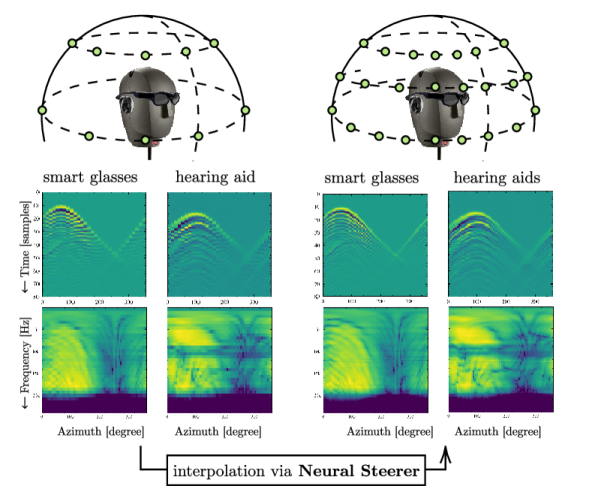
(a) Schematic representation of the proposed Neural Steerer for steering vectors interpolation.

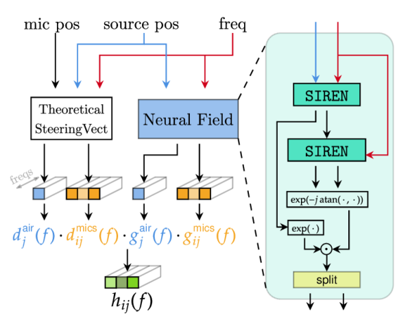
(b) Illustration of the proposed Neural Steerer. Both $\odot$ and $\cdot$ denote element-wise multiplication.

3 Proposed Method

This study aims to model the complex-valued steering vectors as a continuous function of frequency and source location, with a focus on accurately representing the phase information. To this end, we present a physical model and its corresponding Neural Field representation. Finally, we elaborate on the proposed model’s architecture and training objectives.

3.1 Physical Model

Steering vectors encode the direct path sound propagation from a source at position $\mathbf{s}_{j}$ to the microphones at position $\mathbf{m}_{i}$. In the frequency domain, the algebraic model [20] for steering vector $d_{ij}(f)$ at frequency $f$ reads

$$d_{ij}(f)=\exp(-\jmath\omega_{f}r_{ij}/cF_{s})/\sqrt{4\pi}r_{ij},$$ (1)

where $r_{ij}=\|\mathbf{s}_{j}-\mathbf{m}_{i}\|_{2}$ is the source-to-microphone euclidean distance, $c$ is the speed of sounds, $\omega_{f}=2\pi f$ is the angular frequency in frequency band $f$ and $F_{s}$ is the sampling frequency.

In real-world measurement, frequency-dependent filtering effects alter the theoretical shape of the steering vectors. Acoustic simulators then extend (1) by incorporating factors as the propagation in air and microphone directivity [21]. Furthermore, in many applications assuming far-field regime, it is common to operate in spherical coordinates. Therefore, explicating the source-to-reference point distance $r_{j}$, we rewrite the model in terms of source direction of arrival (DoA), represented by azimuth $\theta_{j}$ and elevation $\varphi_{j}$, as

$$h_{ij}(f)=\,g^{\text{air}}_{j}(\theta_{j},\varphi_{j},f)\cdot\!\!\ g^{\text{mic}}_{ij}(\mathbf{m}_{i},\mathbf{r},f)\cdot\underbrace{\exp(-\jmath\omega_{f}\mathbf{n}_{j}^{T}(\mathbf{m}_{i}-\mathbf{r})/c)}_{\triangleq\,d_{ij}^{\text{mic}}(f)},$$ (2)

where $\mathbf{n}_{j}=[\cos\theta_{j}\cos\varphi_{j},\sin\theta_{j}\cos\varphi_{j},\sin\varphi_{j}]^{\top}$ is the unit-norm vector pointing to the $j$-th source [22]. Here, $g_{j}^{\text{air}}(\theta_{j},\varphi_{j},f)$ account for the freq.-dependent air attenuation and eventual source-dependent characteristics, while $g^{\text{mic}}_{ij}(\mathbf{m}_{i},\mathbf{r},f)$ describes the microphone directivity pattern defined with its phase center at $\mathbf{r}$. In general, $g^{\text{mic}}_{ij}(\mathbf{m}_{i},\mathbf{r},f)$ differs for each microphone depending on the type and manufacturing.

3.2 Neural Steerer

The family of steering vector can be represented by the following functional

$$\begin{array}[]{lcccrc}\mathcal{M}:&\mathbb{S}^{2}&\times&\mathbb{R}_{+}&\to&\mathbb{C}\\ &((\theta_{j},\varphi_{j})&,&f)&\mapsto&\;h_{ij}(f)\end{array}$$ (3)

where $\mathbb{S}^{2}$ is the set of spherical polar coordinates on the unit sphere. Note that the dependency on $\mathbf{m}_{i}$ is remove for readability, they are assumed to parameters of the model.

We parameterize $\mathcal{M}$ with a NF, that is a coordinate-based neural network. As discussed in [7], once trained on a finite set of observations, $\mathcal{M}$ can evaluate any input coordinate at arbitrary resolution, whose super-resolution capabilities depends on the network’s inductive bias, e.g. network topology, regularizers, and training data.

Similarly in [18], we model $r_{ij}$ and $\mathbf{m}_{i}$ as a free parameter of the model, which are optimized during training. Then, $d_{j}^{\text{air}}$ and $d_{ij}^{\text{mic}}$ can be computed algebraically from the input coordinated using (2). On one hand, such formulation will provide a good physically-motivated initialization, on the other hand, it will reduce the number of parameters. Therefore, in practice, we predict terms $g^{\text{air}}_{j}(\theta_{j},\varphi_{j},f)$ and $g^{\text{mic}}_{ij}(\mathbf{m}_{i},\mathbf{r},f)$ .

3.3 Network Architecture

The proposed architecture is shown in Fig. 1(b). The neural field (NF) $\mathcal{M}$ is implemented using SIREN [10], a multi-layer perceptron (MLP) with sinusoidal activation functions, as the backbone as in [16]. The NF takes as input the desired source DoA $(\theta_{j},\varphi_{j})$ and frequency $f$ and returns the components of Eq. (2):

$\mathcal{G}_{j}\triangleq\left\{g^{\text{air}}_{j}(\theta_{j},\varphi_{j},f),\{g^{\text{mic}}_{ij}(\mathbf{m}_{i},\mathbf{r},f)\}_{i=1}^{I}\right\}$ , where $I$ is the total number of microphones.

Let $g^{\ast}$ be an entry of $\mathcal{G}_{j}$. Instead of directly predicting the complex-valued $g^{\ast}$ or its real-imaginary parts, we propose to implicitly estimate its magnitude and phase. More precisely, for each $g^{\ast}$, the network returns a $3$-dimensional vector $\mathbf{g}^{\ast}\in\mathbb{R}^{3}$ that is used to obtain $g^{\ast}$ via its magnitude and phase as

$$g^{\ast}=\exp\left(\{\mathbf{g}^{\ast}\}_{1}\right)\,\exp\left(-\jmath 2\pi\arctan\left(\frac{\{\mathbf{g}^{\ast}\}_{2}}{\{\mathbf{g}^{\ast}\}_{3}}\right)\right).$$ (4)

The steering vector $h_{ij}(f)$ is then obtained as in Eq. (2) given $g^{\text{air}}_{j}(\theta_{j},\varphi_{j},f)$ and $g^{\text{mic}}_{ij}(\mathbf{m}_{i},\mathbf{r},f)$ estimated by the NF and the theoretical steering vectors $d_{j}^{\text{air}}(f)$ and $d_{ij}^{\text{mic}}(f)$ computed knowing the microphone positions.

Following the work in [23], we propose an alternative architecture, where the phase estimation is conditioned to the estimation of the magnitude. In practice, the network comprises a cascade of two SIREN: the first one is trained fit the magnitudes of the components from input coordinates, while the second reconstructs the phase based of both coordinates and magnitudes.

The above-proposed model regards frequencies as continuous input variables. In this setting, hereafter referred to as continuous frequency (CF) model, the network output $3\times(I+1)$ real values, 3 being the dimension of $\mathbf{g}^{\ast}$ for handling complex values. In case of discrete frequency (DF) modeling, the last layer of the network is modified to output $3\times(I+1)F$ for a given single source DoA, where $F$ is the total number of frequency regularly sampled in $[0,F_{s}]$, similarly to the DFT operation.

3.4 Training Loss and Off-Grid Regularization

For a given source DoA $(\theta_{j},\varphi_{j})$ and frequency $f$, the neural network is trained to return filters with low phase distortion in both frequency and time domains. Similarly to the loss proposed in [24], we optimize the explicit magnitude and phase errors in the frequency domain plus one explicit term time-domain $\ell_{2}$-loss, that is

$$\begin{split}\mathcal{L}(\hat{h}_{ij}(f),h_{ij}(f))=&\lambda_{1}\mathcal{L}_{\text{LogMag}}(|\hat{h}_{ij}(f)|,|h_{ij}(f)|)\\ +&\lambda_{2}\mathcal{L}_{\text{Phase}}(\angle\hat{h}_{ij}(f),\angle h_{ij}(f))\\ +&\lambda_{3}\|(\text{iDFT}[\hat{h}_{ij}(f)],\text{iDFT}[h_{ij}(f)])\|_{2}^{2}.\end{split}$$ (5)

In practice, as reported in [25], we also find the $\ell_{1}$ loss on the log-magnitude spectrum plus a $\ell_{1}$ loss on the $\cos$ and the $\sin$ of the phase component work best, denoted $\mathcal{L}_{\text{LogMag}}$ and $\mathcal{L}_{\text{Phase}}$, respectively. Moreover, we found empirically that continuous frequencies (CT) is a much harder task than modeling them as discrete output variables. In particular, we found the Neural Field fails at capturing the details across the frequencies dimension, converging towards erroneous solutions. We addressed this pathology by modifying loss functions $\mathcal{L}_{\text{LogMag}}$ and $\mathcal{L}_{\text{Phase}}$ to account for the sequential nature of frequencies as an instance of causal training, as in [26].

The main limitation of the loss in (5) is that it can be evaluated only on training data. Following the training strategies used in PINNs, we can use a physical model to regularize the objective evaluated on source locations at any arbitrary resolution in unsupervised fashion [27, 28].

One of the main requirements is that our estimated steering vector $\hat{h}_{ij}(f)$, and it components, are causal, for every source position. The any anti-causal components may lead to artifacts and incoherent steering vectors. In order to enforce this, we propose to translate a classic relation saying that the imaginary part of the transfer function must be the Hilbert transform $\mathcal{H}$ of the real part of the transfer function as a penalty term, that is

$$\mathcal{L}_{\text{Causal}}=\left\|\mathcal{H}\{\Re[\hat{h}_{ij}(f)]\}-\Im[\hat{h}_{ij}(f)]\right\|_{2}^{2},$$ (6)

where $\Re[\cdot]$ and $\Im[\cdot]$ are the real and imaginary part of the complex argument. Such regularization can be computed straightforwardly in the DF case by sampling randomly source positions in $\mathbb{R}^{3}$. In CF condition, input frequencies need to sampled as well. To simplify the computation of the Hilbert and Fourier transform, we chose to sample a random number of equally-distributed frequencies in $[0,F_{s}]$.

4 Experiments

Table 1: Average RMSE and cosine distance (in parentheses) between the estimated and reference time-domain steering vectors in the steering vector interpolation task. The values average over the 6 channels. * denotes baseline methods.

Freqs	Model	$\mathcal{L}_{\text{MSE}}$	$\lambda_{1}\mathcal{L}_{\text{LogMag}}+\lambda_{2}\mathcal{L}_{\text{Phase}}$	$+\lambda_{3}\mathcal{L}_{\text{iDFT}}$	$+\lambda_{4}\mathcal{L}_{\text{Causal}}$
DF	$\mathtt{SCF}^{*}$	1.42 (0.94)	-	-	-
DF	$\mathtt{SIREN}^{*}$	1.09 (0.80)	-	-	-
DF	$\mathtt{SIREN}_{\text{Phase}}$	1.26 (0.77)	0.36 (0.06)	0.34 (0.06)	0.337 (0.06)
DF	$\mathtt{SIREN}_{\text{Mag}\to\text{Phase}}$	1.22 (0.66)	0.32 (0.05)	0.29 (0.05)	0.284 (0.05)
CF	$\mathtt{SIREN}_{\text{Phase}}$	1.42 (0.88)	0.63 (0.17)	0.58 (0.17)	0.330 (0.06)
CF	$\mathtt{SIREN}_{\text{Mag}\to\text{Phase}}$	1.37 (0.80)	0.53 (0.13)	0.45 (0.09)	0.376 (0.08)

We aimed to obtain a reliable representation of the steering vectors both in the time and frequency domains. Therefore, we wanted to evaluate the performance of the proposed $\mathtt{SIREN}_{\text{Phase}}$ and $\mathtt{SIREN}_{\text{Mag}\to\text{Phase}}$ models in terms of three metrics, i.e., the root mean square error (RMSE) and the cosine distance between the estimated and reference steering vectors in the time domain, and the log-spectral distance (LSD) [dB] between the magnitudes of the estimated and reference HRTFs. We compare our models against a vanilla SIREN, as used in [16] ($\mathtt{SIREN}^{*}$), and an interpolation method based on the spatial characteristic function ($\mathtt{SCF}^{*}$) [6].

Our evaluation used the EasyCom Dataset [1] featuring steering vectors of a 6-channel microphone array consisting of 4 microphones attached to head-worn smart glasses and 2 binaural microphones located in the user’s ear canals. All data were measured at $F_{s}=48\,\text{kHz}$ on a spherical grid with $60$ equally spaced azimuths and $17$ quasi-equally spaced elevations. If not otherwise specified, we consider $F=257$ positive frequencies.

Our $\mathtt{SIREN}_{\text{Phase}}$ and $\mathtt{SIREN}_{\text{Mag}\to\text{Phase}}$ models utilized a SIREN [10] architecture composed of four 512-dimensional hidden layers. Additionally, $\mathtt{SIREN}_{\text{Mag}\to\text{Phase}}$ used a second SIREN featuring two 512-dimensional hidden layers. Those models were trained using a batch size of $B=18$, and a learning rate that is initialized to $10^{-3}$ and scaled by a factor of $0.98$ at every epoch. To avoid overfitting, an early stopping mechanism is applied by monitoring a loss computed on a part (20%) of the training data. In all experiments, we set $\lambda_{1}=\lambda_{4}=1$, and $\lambda_{2}=\lambda_{3}=10$ to match the scale of the different loss terms. $\mathcal{L}_{\text{Causal}}$ is computed using $B$ random coordinates sampled in the unit sphere. The baseline $\mathtt{SIREN}^{*}$ used the same parameterization applied to our $\mathtt{SIREN}_{\text{Phase}}$ model.

We first considered the task of interpolating the steering vector on a regular grid. In this task, the training dataset consisted of steering vectors and locations downsampled regularly by a factor of 2 as in [16]. Table 1 reports the average RMSE and cosine distance of the unseen (missing) data points at full frequency resolution. Our models trained with the proposed regularizers outperformed the baseline in both metrics. Specifically, the performances were improved by introducing new regularization techniques and conditioning the phase estimation on the magnitude. Additionally, in the context of continuous frequency modeling, incorporating the off-grid regularizer $\mathcal{L}_{\text{Causal}}$ results in comparable reconstruction results to those achieved through discrete frequency modeling (with a p-value of $0.0032$).

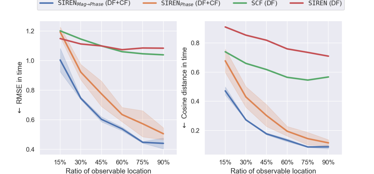
(a) Only unseen test locations

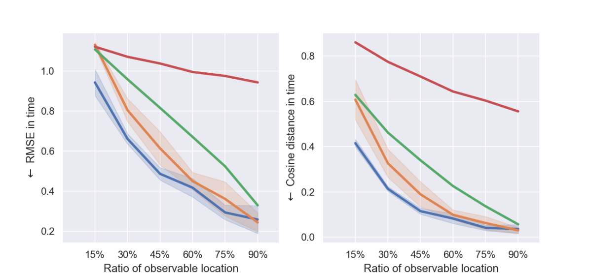
(b) Whole data point locations

Figure 2: RMSE (left) and cosine distance (right) of time-domain steering vectors for unseen locations in the test set (2(a)) and the whole sphere reconstruction on random data (2(b)). Shaded region show the confidence interval for both continuous and discrete frequency models.

Subsequently, we analyzed the reconstruction capabilities as a function of available points (in percentage) randomly sampled from the original grid. Fig. 2 displays the two time-domain objectives for the unseen data only (top) and on the full test dataset (bottom), which comprises training and unseen data points. The curves reaffirm the results discussed earlier, showing that conditioning phase estimation by magnitude estimates yields better results. Notably, it can be observed that the $\texttt{SIREN}^{*}$ model trained solely to minimize the $\ell_{2}$ norm in the complex domain exhibits suboptimal performance in the reconstruction of both seen and unseen points, even when 90$\%$ of the points are seen during training.

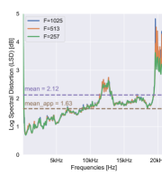
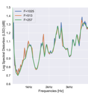
Figure 3: Average log-spectral distortion at different resolutions in the whole (left) and a selected (right) frequency range. The model was trained on $F=257$ frequency bins.

Finally, we analyzed the interpolation performances along the frequency axis. Specifically, we trained a CF variant of $\mathtt{SIREN}_{\text{Mag}\to\text{Phase}}$ model to fit steering vectors measured at $F=257$ frequencies and then evaluated at varying spectral resolutions. The obtained results, presented in Fig. 3, demonstrate that the reconstruction error remains consistently low across different evaluation grids. However, it should be noted that the errors increase with the frequency and become more pronounced at the boundaries. This observation could be attributed to the band-limited nature of the target signal. It was also in line with previous findings reported in [16]. Nevertheless, within the frequency range commonly utilized in classical speech processing applications, namely $f\in[40,20000]$ Hz, the mean LSD was approximately 0.5 dB lower.

5 Conclusion

In this paper, we have proposed a novel neural field model that encodes the steering vector continuously over both spatial and frequency coordinates, given discrete measurements. Our approach places particular emphasis on accurately capturing the phase component of the target filters, while enforcing that the filters maintain their causal nature. We have demonstrated the effectiveness of our model in reconstructing real measurements of steering vectors. Moving forward, we plan to investigate the potential applications of this model in a broad range of scenarios, including source localization and separation.

References

- [1] Jacob Donley, Vladimir Tourbabin, Jung-Suk Lee, Mark Broyles, Hao Jiang, Jie Shen, Maja Pantic, Vamsi Krishna Ithapu, and Ravish Mehra. EasyCom: An augmented reality dataset to support algorithms for easy communication in noisy environments. arXiv e-print, 2021. arXiv:2107.04174v2.
- [2] Kouhei Sekiguchi, Yoshiaki Bando, Aditya Arie Nugraha, Kazuyoshi Yoshii, and Tatsuya Kawahara. Fast multichannel nonnegative matrix factorization with directivity-aware jointly-diagonalizable spatial covariance matrices for blind source separation. IEEE/ACM Trans. Audio, Speech, Language Process., 28:2610–2625, 2020.
- [3] Ralph Schmidt. Multiple emitter location and signal parameter estimation. IEEE Trans. Antennas Propag., 34(3):276–280, 1986.
- [4] Paolo Annibale, Jason Filos, Patrick A Naylor, and Rudolf Rabenstein. Geometric inference of the room geometry under temperature variations. In Proc. Int. Symp. Control Commmun. Signal Process., pages 1–4, 2012.
- [5] Sharon Gannot, David Burshtein, and Ehud Weinstein. Signal enhancement using beamforming and nonstationarity with applications to speech. IEEE Trans. Signal Process., 49(8):1614–1626, 2001.
- [6] Fábio P. Freeland, Luiz W. P. Biscainho, and Paulo S. R. Diniz. Interpolation of head-related transfer functions (HRTFS): A multi-source approach. In Proc. Eur. Signal Process. Conf., pages 1761–1764, 2004.
- [7] Yiheng Xie, Towaki Takikawa, Shunsuke Saito, Or Litany, Shiqin Yan, Numair Khan, Federico Tombari, James Tompkin, Vincent Sitzmann, and Srinath Sridhar. Neural fields in visual computing and beyond. In Computer Graphics Forum, volume 41, pages 641–676, 2022.
- [8] Dmitry N. Zotkin, Ramani Duraiswami, and Nail A. Gumerov. Regularized HRTF fitting using spherical harmonics. In Proc. IEEE Workshop Appl. Signal Process. Audio Acoust., pages 257–260, 2009.
- [9] Ben Mildenhall, Pratul P. Srinivasan, Matthew Tancik, Jonathan T. Barron, Ravi Ramamoorthi, and Ren Ng. NeRF: Representing scenes as neural radiance fields for view synthesis. In Proc. Eur. Conf. Comput. Vis., pages 405–421, 2020.
- [10] Vincent Sitzmann, Julien Martel, Alexander Bergman, David Lindell, and Gordon Wetzstein. Implicit neural representations with periodic activation functions. In Proc. Neural Inf. Process. Syst., pages 7462–7473, 2020.
- [11] Emilien Dupont, Adam Goliński, Milad Alizadeh, Yee Whye Teh, and Arnaud Doucet. COIN: Compression with implicit neural representations. arXiv e-print, 2021. arXiv:2103.03123v2.
- [12] Guy Gafni, Justus Thies, Michael Zollhofer, and Matthias Nießner. Dynamic neural radiance fields for monocular 4D facial avatar reconstruction. In Proc. IEEE/CVF Conf. Comput. Vis. Pattern Recog., pages 8649–8658, 2021.
- [13] Maziar Raissi, Paris Perdikaris, and George E. Karniadakis. Physics-informed neural networks: A deep learning framework for solving forward and inverse problems involving nonlinear partial differential equations. J. Comput. Phys., 378:686–707, 2019.
- [14] George Em Karniadakis, Ioannis G Kevrekidis, Lu Lu, Paris Perdikaris, Sifan Wang, and Liu Yang. Physics-informed machine learning. Nature Reviews Phys., 3(6):422–440, 2021.
- [15] Alexander Richard, Peter Dodds, and Vamsi Krishna Ithapu. Deep impulse responses: Estimating and parameterizing filters with deep networks. In Proc. IEEE Int. Conf. Acoust., Speech, Signal Process., pages 3209–3213, 2022.
- [16] You Zhang, Yuxiang Wang, and Zhiyao Duan. HRTF field: Unifying measured HRTF magnitude representation with neural fields. In Proc. IEEE Int. Conf. Acoust., Speech, Signal Process., 2023. accepted, arXiv:2210.15196v3.
- [17] Jin Woo Lee, Sungho Lee, and Kyogu Lee. Global HRTF interpolation via learned affine transformation of hyper-conditioned features. In Proc. IEEE Int. Conf. Acoust., Speech, Signal Process., 2023. submitted, arXiv:2204.02637v2.
- [18] Jin Woo Lee and Kyogu Lee. Neural fourier shift for binaural speech rendering. In Proc. IEEE Int. Conf. Acoust., Speech, Signal Process., 2023. submitted, arXiv:2211.00878v1.
- [19] Andrew Luo, Yilun Du, Michael J Tarr, Joshua B Tenenbaum, Antonio Torralba, and Chuang Gan. Learning neural acoustic fields. In Proc. Neural Inf. Process. Syst., pages 1–13, 2022.
- [20] Heinrich Kuttruff. Room Acoustics. CRC Press, 6 edition, 2016.
- [21] Robin Scheibler, Eric Bezzam, and Ivan Dokmanić. Pyroomacoustics: A python package for audio room simulation and array processing algorithms. In Proc. IEEE Int. Conf. Acoust., Speech, Signal Process., pages 351–355, 2018.
- [22] Emmanuel Vincent, Tuomas Virtanen, and Sharon Gannot. Audio Source Separation and Speech Enhancement. John Wiley & Sons, 2018.
- [23] Aditya Arie Nugraha, Kouhei Sekiguchi, and Kazuyoshi Yoshii. A deep generative model of speech complex spectrograms. In Proc. IEEE Int. Conf. Acoust., Speech, Signal Process., pages 905–909, 2019.
- [24] Alexander Richard, Dejan Markovic, Israel D. Gebru, Steven Krenn, Gladstone Alexander Butler, Fernando Torre, and Yaser Sheikh. Neural synthesis of binaural speech from mono audio. In Proc. Int. Conf. Learn. Representations, pages 1–13, 2021.
- [25] Jacob Donley and Paul Calamia. DARE-Net: Speech dereverberation and room impulse response estimation. Technical report, Stanford University, 2022.
- [26] Sifan Wang, Shyam Sankaran, and Paris Perdikaris. Respecting causality is all you need for training physics-informed neural networks. arXiv e-print, 2022. arXiv:2203.07404v1.
- [27] Diego Di Carlo, Dominique Heitz, and Thomas Corpetti. Post processing sparse and instantaneous 2D velocity fields using physics-informed neural networks. In Proc. Int. Symp. Appl. Laser Imag. Tech. Fluid Mech., pages 1–11, 2022.
- [28] Sifan Wang, Yujun Teng, and Paris Perdikaris. Understanding and mitigating gradient flow pathologies in physics-informed neural networks. SIAM J. Sci. Comput., 43(5):A3055–A3081, 2021.