Controlling superconducting transistor by coherent light

Abstract

The Josephson junction is typically tuned by a magnetic field or electrostatic gates to realize a superconducting transistor, which manipulates the supercurrent in integrated superconducting circuits. However, this tunable method does not achieve simultaneous control for the supercurrent phase (phase difference between two superconductors) and magnitude. Here, we propose a novel scheme for the light-controlled superconducting transistor, which is composed of two superconductor leads linked by a coherent light-driven quantum dot. We discover a Josephson-like relation for supercurrent $I_{\mathrm{s}}=I_{c}(\Phi)\,\sin\Phi$, where both supercurrent phase $\Phi$ and magnitude $I_{c}$ could be entirely controlled by the phase, intensity, and detuning of the driving light. Additionally, the supercurrent magnitude displays a Fano profile with the increase of the driving light intensity, which is clearly understood by comparing the level splitting of the quantum dot under light driving and the superconducting gap. Moreover, when two such superconducting transistors form a loop, they make up a light-controlled superconducting quantum interference device (SQUID). Such a light-controlled SQUID could demonstrate the Josephson diode effect, and the optimized non-reciprocal efficiency achieves up to $54\%$, surpassing the maximum record reported in recent literature. Thus, our feasible scheme delivers a promising platform to perform diverse and flexible manipulations in superconducting circuits.

Introduction - Semiconductor transistor lies in the fundamental position in modern electronics. Analogous to it, superconducting transistors, which can control superconducting current (Ando et al., 2020; Daido et al., 2022; Baumgartner et al., 2022; Bauriedl et al., 2022; Wu et al., 2022; Jarillo-Herrero et al., 2006; Franceschi et al., 2010), are attracting more and more attentions, since they have lower power consumption, and may provide potential applications for quantum information processing (Clarke and Wilhelm, 2008). Recently, superconducting transistors based on Josephson junction microstructures (Hu et al., 2007; Misaki and Nagaosa, 2021; Wu et al., 2022) and the superconducting quantum interferometer devices (SQUID) (Szombati et al., 2016; Fominov and Mikhailov, 2022; Souto et al., 2022) already have implemented to rectify (significant non-reciprocal supercurrent), switch (Doh et al., 2005; Jarillo-Herrero et al., 2006; Winkelmann et al., 2009; Katsaros et al., 2010; Bobkova et al., 2021) and reverse (Baselmans et al., 1999; Rozhkov et al., 2001; Razmadze et al., 2020) the supercurrent (van Dam et al., 2006; Franceschi et al., 2010; Paolucci et al., 2019). Usually, such devices need to be controlled by an external magnetic field or/and electrostatic voltage, to our knowledge, which are the only two kinds of available control methods thus far (Jarillo-Herrero et al., 2006; Baumgartner et al., 2022; Davydova et al., 2022; Zhang et al., 2022). However, a concise scheme of the superconducting transistor based on the Josephson junction by the above two tunable methods to simultaneously control the supercurrent switch, reverse, phase (the phase difference between two superconductors), and magnitude (critical current), has yet to be proposed.

In this letter, we propose a novel scheme for the superconducting transistor which is coherently controlled by light. The system is composed of two superconductor leads linked by a light-driven quantum dot (QD) with two levels [Fig. 1 (a)], which is similar to a single-photon transistor based on superconducting transmission line resonators and qubits (Zhou et al., 2008). When there is no driving light, the supercurrent is switched off, while it is switched on under proper driving light intensity. More importantly, it turns out the supercurrent passing through the transistor depends not only on the driving light intensity, but also on the phase $\phi_{\mathrm{d}}$ of the coherent light, as well as the superconductor phase difference $\varDelta\varphi_{\mathrm{s}}$ between the two leads, which gives $I_{\mathrm{s}}=I_{c}(\Phi)\,\sin\Phi$, with $\Phi:=\varDelta\varphi_{\mathrm{s}}+2\phi_{\mathrm{d}}$. In this sense, we refer to it as the light-controlled dc Josephson effect.

Moreover, it is intriguing that the critical current $I_{c}$ achieve complete reversal by adjusting the detuning and driving intensity of light, which implements a light-controlled $\pi$-junction in Fig. 1 (c) (Baselmans et al., 1999; Rozhkov et al., 2001; Zhu et al., 2002a; van Dam et al., 2006; Razmadze et al., 2020; Whiticar et al., 2021; Karan et al., 2022; Bargerbos et al., 2022). Remarkably, the critical current $I_{c}$ here exhibits a Fano dependence on the driving light intensity with the fixed light detuning [see Fig. 1 (d)]. Namely, with the increase of the driving light intensity, the critical current $I_{c}$ first increases in the positive direction, but then decreases down to zero and increases in the negative direction, finally $I_{c}$ drops back and approaches zero. From the resonance comparison between the QD levels subjected to driving light and the superconductor band spectrum, we obtain a clear picture to understand this result.

Further, an interference loop is formed by such two superconducting transistors, and the light fields applied on the two QDs generate a phase difference depending on their spatial distance. As a result, the supercurrents passing through such an interference loop forward and backward turn out to be asymmetric with each other, and a light-controlled Josephson diode is achieved. It turns out the optimal nonreciprocity of such a Josephson diode reaches $54\%$ by properly adjusting the light intensity, which exceeds the best record reported up to now ($\sim 40\%$) (Davydova et al., 2022; Souto et al., 2022).

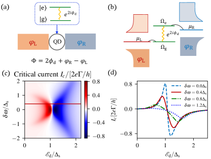
Figure 1: (a) Two superconductors are linked by a light-driven quantum dot with two levels, whose levels are illustrated in (b). (c) The change of critical current $I_{c}$ with the the driving strength $\mathcal{E}_{\mathrm{d}}$ and the light detuning $\delta\omega$. (d) The critical current $I_{c}$ as the driving strength $\mathcal{E}_{\mathrm{d}}$ increase shows the Fano profile with the fixed light detuning $\mathrm{\delta\omega=0,0.4,0.8,1.2\Delta_{\mathrm{s}}}$. Hereafter, the same coupling strength always are set as $\Gamma_{\mathrm{L}}=\Gamma_{\mathrm{R}}=\Gamma=0.1\Delta_{\mathrm{s}}$.

Superconducting transistor setup - The setup of the superconducting transistor is demonstrated in Fig. 1 (a), which is composed of a two-level QD in contact with two s-wave superconductor leads. Denoting $\Delta_{\mathrm{n}}\equiv|\Delta_{\mathrm{n}}|e^{i\varphi_{\mathrm{n}}}$ and $\mu_{\mathrm{n}}$ as the pairing strength and chemical potential of the two leads $\mathrm{n}=\mathrm{L},\mathrm{R}$, the Hamiltonian of lead-$\mathrm{n}$ is described by (Cuevas et al., 1996; Zhu et al., 2002b)

$$H_{\mathrm{n}}=\sum_{\mathbf{k\sigma}}(\epsilon_{\mathrm{n},\mathbf{k}}+\mu_{\mathrm{n}})c_{\mathrm{n},\mathbf{k}\sigma}^{\dagger}c_{\mathrm{n},\mathbf{k}\sigma}+[e^{2i\mu_{\mathrm{n}}t}\Delta_{\mathrm{n}}^{*}c_{\mathrm{n},-\mathbf{k}\downarrow}c_{\mathrm{n},\mathbf{k}\uparrow}+\mathrm{H.c.}]$$ (1)

with the index for spin $\sigma=\uparrow,\,\downarrow$. Hereafter, we consider the two leads have $|\Delta_{\mathrm{R}}|=|\Delta_{\mathrm{L}}|:=\Delta_{\mathrm{s}}$, but different phases $\varphi_{\mathrm{R,L}}$ and chemical potentials $\mu_{\mathrm{R,L}}$.

The two leads are linked by a QD with two fermionic levels (Recher et al., 2010; Katsaros et al., 2010), which is described by $H_{0}=\sum_{\sigma}\,\Omega_{\mathrm{e}}\,d_{\mathrm{e}\sigma}^{\dagger}d_{\mathrm{e}\sigma}+\Omega_{\mathrm{g}}\,d_{\mathrm{g}\sigma}^{\dagger}d_{\mathrm{g}\sigma}$ ($\Omega_{\mathrm{e}}\geq\Omega_{\mathrm{g}}$). And, the electrons tunnel between the QD and the two leads via the interaction

$$H_{t}=-\sum_{\mathrm{i}=\mathrm{g,e}}\sum_{\mathrm{n},\mathbf{k},\sigma}\big{(}\mathrm{t}_{\mathrm{n,i},\mathbf{k}}d_{\mathrm{i}\sigma}^{\dagger}c_{\mathrm{n},\mathbf{k}\sigma}+\mathrm{t}_{\mathrm{n,i},\mathbf{k}}^{*}c_{\mathrm{n},\mathbf{k}\sigma}^{\dagger}d_{\mathrm{i}\sigma}\big{)}.$$ (2)

In the interaction picture, the tunneling terms between the upper (lower) level and lead-L(R) would contain a fast oscillating factor, and they could be omitted by the rotating wave approximation [See Appendix B]. Thus, equivalently the upper (lower) level is only contacted with the right (left) lead [see Fig. 1 (b)].

Because of the separation of the QD, no supercurrent could flow between the two superconducting leads. However, a tunneling bridge could be built up when a monochromatic coherent light (with frequency $\omega_{\mathrm{d}}$) is injected on the QD, which drives the electron up and down between the two QD levels: $V_{\mathrm{d}}=\sum_{\sigma}\,\mathcal{E}_{\mathrm{d}}\,d_{\mathrm{e}\sigma}^{\dagger}d_{\mathrm{g}\sigma}e^{-i\omega_{\mathrm{d}}t-i\phi_{\mathrm{d}}}+\mathrm{H.c.}$ Here, $\phi_{\mathrm{d}}$ comes from the phase of the coherent light, $\mathcal{E}_{\mathrm{d}}$ is taken as a positive and real driving strength, and $|\mathcal{E}_{\mathrm{d}}|^{2}$ is proportional to the light intensity.

Light-controlled dc Josephson effect - In the rotating frame applied by the unitary transformation $\mathbf{U}(t)=\exp[i(N_{\mathrm{L}}+\sum_{\sigma}d_{\mathrm{g}\sigma}^{\dagger}d_{\mathrm{g}\sigma})\mu_{\mathrm{L}}t+i(N_{\mathrm{R}}+\sum_{\sigma}d_{\mathrm{e}\sigma}^{\dagger}d_{\mathrm{e}\sigma})(\mu_{\mathrm{R}}t+\phi_{\mathrm{d}})]$ with $N_{\mathrm{n}}=\sum_{\mathbf{k\sigma}}c_{\mathrm{n},\mathbf{k}\sigma}^{\dagger}c_{\mathrm{n},\mathbf{k}\sigma}$, the Hamiltonian of the QD under coherent driving becomes

$$\bar{H}_{\text{{qd}}}=\sum_{\mathrm{i,}\sigma}\bar{\Omega}_{\mathrm{i}}d_{\mathrm{i}\sigma}^{\dagger}d_{\mathrm{i}\sigma}-(\mathcal{E}_{\mathrm{d}}d_{\mathrm{e}\sigma}^{\dagger}d_{\mathrm{g}\sigma}e^{i(\mu_{\mathrm{R}}-\mu_{\mathrm{L}}-\omega_{\mathrm{d}})t}+\mathrm{H.c.})$$ (3)

with the reduced upper (lower) level $\bar{\Omega}_{\mathrm{e}(\mathrm{g})}:=\Omega_{\mathrm{e}(\mathrm{g})}-\mu_{\mathrm{R}(\mathrm{L})}$.

Meanwhile, in this rotating frame, the Hamiltonian (1) for the two leads become time-independent, meaning that the effective chemical potentials of two superconducting leads are regarded as $\bar{\mu}_{\mathrm{L}}=\bar{\mu}_{\mathrm{R}}=0$ , and the phases of the two superconducting leads are also corrected as $\bar{\varphi}_{\mathrm{R}}=\varphi_{\mathrm{R}}+2\phi_{\mathrm{d}}$ and $\varphi_{\mathrm{L}}$ [see Fig. 2(a)]. Further, if we focus on the situation that $\omega_{\mathrm{d}}=\mu_{\mathrm{R}}-\mu_{\mathrm{L}}$, namely, the driving frequency is equal to the voltage difference, and thus the Hamiltonian (3) also becomes time-independent.

Based on this time-independent model in the rotating frame, by calculating the evolution of the Green functions of this system, the supercurrent through the superconducting transistor induced by the driving light is exactly obtained as

$$I_{\mathrm{s}}=I_{c}(\Phi)\sin(\Phi),$$ (4)

where the verbose critical current $I_{c}$ is explicitly given in Appendix B. Especially, here $\Phi$ is a phase difference defined by

$$\Phi:=\bar{\varphi}_{\mathrm{R}}-\varphi_{\mathrm{L}}=\varphi_{\mathrm{R}}-\varphi_{\mathrm{L}}+2\phi_{\mathrm{d}}.$$ (5)

It is worth noting that the above supercurrent follows the Josephson-like relation, but here $\Phi$ incorporates not only the phase difference from the two superconducting leads $\varDelta\varphi_{\mathrm{s}}\equiv\varphi_{\mathrm{R}}-\varphi_{\mathrm{L}}$, but also an additional correction from the light phase $\phi_{\mathrm{d}}$ which was previously attainable only by a magnetic field passing through the junction (Tinkham, 2004). Hereafter, we set $\mu_{\mathrm{R}}\geq\mu_{\mathrm{L}}=\Omega_{\mathrm{g}}\equiv 0$ as the energy reference and define the detuning between the driving frequency $\omega_{\mathrm{d}}$ and the energy gap of the two QD levels (light detuning) as $\delta\omega=(\Omega_{\mathrm{e}}-\Omega_{\mathrm{g}})-\omega_{\mathrm{d}}$.

In the large detuning situation ($\delta\omega\gg\mathcal{E}_{\mathrm{d}}$), the above critical current $I_{c}(\Phi)\simeq I_{c}$ becomes a constant independent of the phase difference $\Phi$, then the above supercurrent (4) is simplified as $I_{\mathrm{s}}=I_{c}\sin\Phi$ [see Appendix B]. This result well returns the same form as the dc Josephson effect (Josephson, 1962), except here $\Phi$ is corrected by the light phase $\phi_{\mathrm{d}}$.

On the other hand, it is evident that the critical current $I_{c}(\Phi)$ is also highly dependent on the driving strength $\mathcal{E}_{\mathrm{d}}$, or the driving light intensity. When there is no driving light ($\mathcal{E}_{\mathrm{d}}=0$), no supercurrent flows across the two leads $I_{\mathrm{s}}=0$, which is consistent with our previous discussion. As displayed in Fig. 2 (b), the critical current $I_{c}$ depending on the driving strength $\mathcal{E}_{\mathrm{d}}$ as well as the detuning $\delta\omega$ (here the total phase difference is set as $\Phi=\pi/2$) appears as a butterfly-like shape. Notably, when the detuning is fixed as $\delta\omega=0.4\Delta_{\mathrm{s}}$ [solid red line of Fig. 1 (c)], the critical current $I_{c}$ exhibits a Fano profile depending on the driving strength $\mathcal{E}_{\mathrm{d}}$ [Fig. 1 (d)], which could be fully reversed in both positive and negative directions. In this case, this superconducting transistor achieves a $\pi$-junction controlled by the light intensity (Baselmans et al., 1999; Rozhkov et al., 2001; Zhu et al., 2002a; van Dam et al., 2006; Razmadze et al., 2020; Whiticar et al., 2021; Karan et al., 2022; Bargerbos et al., 2022).

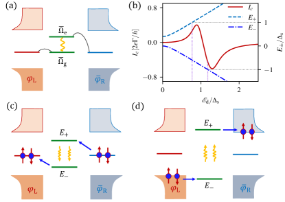
Figure 2: (a) The level distribution of the superconducting transistor setup in the rotating frame. (b) The split of energy levels $E_{+}$ (dashed line) and $E_{-}$ (dashdotted line) of QD with the driving strength $\mathcal{E}_{\mathrm{d}}$ increase. The intersections of the purple and gray dotted lines corresponds to $E_{\pm}=\Delta_{\mathrm{s}}$. The Fano profile of critical current is because the flow direction of Cooper pairs reverses the back [from lead-R to lead-L in (c)] and forth [from lead-L to lead-R in (d)] between two superconducting leads with increasing driving strength.

Fano dependence of the critical current - Unexpectedly, as the driving light increases, the critical current does not increase, but exhibits a Fano profile as depicted in Fig. 2 (b), which has been observed in controllable single-photon transistors as well (Zhou et al., 2008). And this Fano profile is elucidated by considering the weak coupling limit $\Gamma\ll\Delta_{\mathrm{s}}$, which allows us to neglect high order terms $\Gamma/\Delta_{\mathrm{s}}$. In this limit, the critical current (4) is reduced to

$$I_{c}\simeq\int\mathrm{d}\nu\frac{e\Gamma\sqrt{\gamma_{\mathrm{s}}(\nu)}\Delta_{\mathrm{s}}^{2}\mathcal{E}_{\mathrm{d}}^{2}}{h\left[2\nu^{2}-\Omega^{2}\right]\nu^{2}}\frac{\Gamma^{2}}{\Gamma^{2}+\frac{\gamma_{\mathrm{s}}^{2}(\nu)(\nu^{2}-E_{+}^{2})^{2}(\nu^{2}-E_{-}^{2})^{2}}{\nu^{4}\left((\nu^{2}-E_{+}^{2})+(\nu^{2}-E_{-}^{2})\right)^{2}}},$$ (6)

with $\gamma_{\mathrm{s}}(\nu)=\sqrt{\nu^{2}-\Delta_{\mathrm{s}}^{2}}$ and $\Omega^{2}=2(\delta\omega^{2}+2\mathcal{E}_{\mathrm{d}}^{2})$. And, the QD levels are obtained by diagonalizing the Hamiltonian (3) of light-driven QD as $E_{\pm}=(1/2)(\delta\omega\pm\sqrt{\delta\omega^{2}+4\mathcal{E}_{\mathrm{d}}^{2}})$. By taking into account the main contribution of the integral (6) near $\nu\simeq-\Delta_{\mathrm{s}}-\varepsilon$ ($\varepsilon$ is infinitesimal) due to $(\nu^{2}-\Delta^{2})^{-\frac{1}{2}}\rightarrow\infty$, thus the critical current is approximated as

$$I_{c}\simeq\frac{2e\Gamma}{h}\frac{\mathcal{E}_{\mathrm{d}}^{2}(2\varepsilon\Delta_{\mathrm{s}})^{-\frac{1}{2}}}{2\Delta_{\mathrm{s}}^{2}-\Omega^{2}}\frac{\Gamma^{2}}{\Gamma^{2}+\frac{2\varepsilon(\Delta_{\mathrm{s}}^{2}-E_{+}^{2})^{2}(\Delta_{\mathrm{s}}^{2}-E_{-}^{2})^{2}}{\Delta_{\mathrm{s}}^{3}\left((\Delta^{2}-E_{+}^{2})+(\Delta^{2}-E_{-}^{2})\right)^{2}}}.$$ (7)

And numerical computation reveals that the aforementioned approximation is reasonable [see Appendix B]. Notice that, as the driving strength increase, the critical current $(\ref{eq:simplied_DC_2})$ appears with two resonance peaks corresponding to $E_{\pm}=\Delta_{\mathrm{s}}$, the positive (negative) of which is determined by the sign of $2\Delta_{\mathrm{s}}^{2}-(\delta\omega^{2}+2\mathcal{E}_{\mathrm{d}}^{2})$.

Specifically, when the driving light intensity is weak, the two QD levels are positioned beneath the superconducting gap [Fig. 2 (c)], effectively creating Andreev bound states (Zagoskin, 2014). These two states serves as a pathway for supercurrent transport, whereby the Cooper pair flows from the lead-R into the upper QD level through the Andreev reflection (AR), then transitions to the lower QD level via light emission, and finally flows into the lead-L by AR again [Fig. 2 (c)]. Meanwhile, the critical current is positive due to $2\Delta_{\mathrm{s}}^{2}-(\delta\omega^{2}+2\mathcal{E}_{\mathrm{d}}^{2})>0$.

As the intensity of the driving light further increases, one of the two QD levels will be adjacent to the superconducting continuum spectrum, resulting in the emergence of a resonant peak of positive critical current. However, when one of two QD levels surpasses the superconducting gap, the positive critical current gradually decreases zero at $\mathcal{E}_{\mathrm{d}}^{2}=\Delta_{\mathrm{s}}^{2}-\delta\omega^{2}/2$ and even reverse as AR is further suppressed. Once both QD levels surpass the superconducting gap [Fig. 2 (d)], the supercurrent increases negatively, and another resonance peak of negative critical current appears. At this point, Cooper pair flows from lead-L to the lower QD level, then driven by light to the upper QD level and finally transports into the continuous band of lead-R [Fig. 2 (d)].

The above physical picture have also been justified. As shown in Fig. 2 (b), the driving strength $\mathcal{E}_{\mathrm{d}}^{\pm}$ corresponding to the intersection point of $E_{\pm}(\mathcal{E}_{\mathrm{d}})=\pm\Delta_{\mathrm{s}}$ [two dotted purple lines in Fig. 2 (b)] and the position $\mathcal{E}_{\mathrm{peak}}^{\pm}$ of two resonant peaks of the critical current $I_{c}(\mathcal{E}_{\mathrm{peak}})$ are approximately equal within the range of $\Gamma$ error, i.e., $|\mathcal{E}_{\mathrm{d}}^{\pm}-\mathcal{E}_{\mathrm{peak}}^{\pm}|\leq\Gamma$. And the deviation of the approximate theory analysis using Eq. (7) and the accurate numerical computation is ascribed to the application of the weak coupling condition $\Gamma\ll\Delta_{\mathrm{s}}$ and exclusive consideration of the primary contribution of the integral near $\nu\sim-\Delta_{\mathrm{s}}$.

Light-controlled SQUID - Furthermore, if two such superconducting transistors are placed nearby and forms a loop, they make up a SQUID which is also coherently controlled by light (Recher et al., 2010; Godschalk and Nazarov, 2014; Bouscher et al., 2017) [Fig. 3 (a)]. The current through the SQUID sums up the contributions through each QD, $I_{\mathrm{s}}=I_{\mathrm{s},1}+I_{\mathrm{s},2}$, where the current $I_{\mathrm{s},i}$ through QD-$i$ is given by the modified Josephson relation (4). Under a proper driving light intensity ($\mathcal{E}_{\mathrm{d}}\ll\delta\omega$), the current through the SQUID gives [see Appendix C]

$$I_{\mathrm{s}}\simeq I_{c,1}\sin(\varDelta\varphi_{\mathrm{s}}+2\phi_{\mathrm{d},1})+I_{c,2}\sin(\varDelta\varphi_{\mathrm{s}}+2\phi_{\mathrm{d},2}),$$ (8)

with the phase difference between two superconductors $\varDelta\varphi_{\mathrm{s}}\equiv\varphi_{\mathrm{R}}-\varphi_{\mathrm{L}}$ and the phase $\phi_{\mathrm{d},i}$ of driving light applied to QD-$i$. Here we consider the light fields applied on the two QDs originate from the same point source, thus they have a deterministic phase difference which is determined by their optical paths $\varDelta\phi_{\mathrm{d}}\equiv\phi_{\mathrm{d},2}-\phi_{\mathrm{d},1}$ [see Fig. 3(a)].

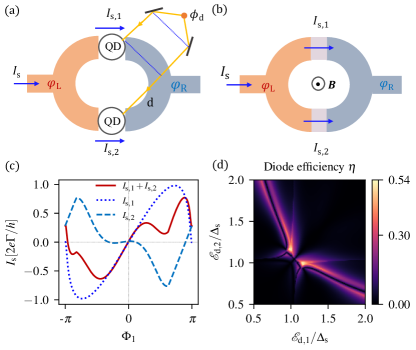
Figure 3: The supercurrent through superconducting quantum interference device controlled by the coherent light (a) and the magnetic field (b). (c) The total phase-asymmetric current (red solid line) is sum of the phase-symmetric current (blue dotted line) through QD-$1$ and the phase-symmetric current (light blue dashed line) through QD-$2$ with the driving strength $\mathcal{E}_{\mathrm{d},1}=1.0\Delta_{\mathrm{s}}$ and $\mathcal{E}_{\mathrm{d},2}=1.1\Delta_{\mathrm{s}}$. (d) Diode efficiency $\eta$ versus driving strength $\mathcal{E}_{\mathrm{d},1}$ and $\mathcal{E}_{\mathrm{d},2}$ for QD-$1$ and QD-$2$. The optical phase difference and light detuning have set: $\varDelta\phi_{\mathrm{d}}=\pi/10$ and $\delta\omega=0$.

If the light intensities applied on the two QDs are equal, they give equal critical currents $I_{c,1}=I_{c,2}\equiv I_{c}$, and then the supercurrent through the SQUID becomes $I_{\mathrm{s}}=2I_{c}\sin(\varDelta\varphi_{\mathrm{s}}+\phi_{\mathrm{d},1}+\phi_{\mathrm{d},2})\cos\varDelta\phi_{\mathrm{d}}$. This is similar to the SQUID controlled by the magnetic flux [Fig. 3 (b)] (Tinkham, 2004). The sinusoidal oscillation of the supercurrent adjusted by changing the optical path difference provides a method to set a comparison reference between the superconducting phase and the light phase.

More generally, if the light intensities applied on the two QDs are not equal to each other and generate different critical currents $I_{c,1}(\mathcal{E}_{\mathrm{d},1},\phi_{\mathrm{d},1})\neq I_{c,2}(\mathcal{E}_{\mathrm{d},2},\phi_{\mathrm{d},2})$, it turns out such a SQUID gives an asymmetric current-phase relation (Golubov et al., 2004), which can be utilized to realize a Josephson diode (Souto et al., 2022). From the Josephson relation (4), it can be verified that the current through QD-$1$ $I_{\mathrm{s},1}=I_{c,1}(\Phi_{1})\sin\Phi_{1}$ is an odd function of $\Phi_{1}=\varDelta\varphi_{\mathrm{s}}+2\phi_{\mathrm{d},1}$, since $I_{c,1}(\Phi_{1})=I_{c,1}(-\Phi_{1})$ is even; in contrast, because of the optical phase difference $\varDelta\phi_{\mathrm{d}}$, the current through QD-2 $I_{\mathrm{s},2}(\Phi_{2}\equiv\Phi_{1}+2\varDelta\phi_{\mathrm{d}})$ is asymmetric of $\Phi_{1}$ [see Fig. 3(c)].

As a result, summing up $I_{\mathrm{s},1}$ and $I_{\mathrm{s},2}$, the maximum currents through the SQUID in the two directions are different, $|I_{\mathrm{s},max}^{+}|\neq|I_{\mathrm{s},max}^{-}|$ [Fig. 3 (c)], which makes the SQUID a diode. To quantify the non-reciprocity of the diode, we adopt the following diode efficiency (Davydova et al., 2022; Souto et al., 2022)

$$\eta=\frac{\left||I_{\mathrm{s},max}^{+}|-|I_{\mathrm{s},max}^{-}|\right|}{|I_{\mathrm{s},max}^{+}|+|I_{\mathrm{s},max}^{-}|}.$$ (9)

We find that, when the optical path difference is set as $\varDelta\phi_{\mathrm{d}}\simeq 0.1\pi$, and the driving strengths applied on the two QDs are set as $\mathcal{E}_{\mathrm{d},1}\simeq 0.99\Delta_{\mathrm{s}}$, $\mathcal{E}_{\mathrm{d},2}\simeq 1.16\Delta_{\mathrm{s}}$, the above diode efficiency achieves its maximum $\eta\simeq 53.9\%$ [see Fig. 3 (d)]. This is greater than the best record reported in literature ($\sim 40\%$), which was controlled by magnetic field (Davydova et al., 2022; Souto et al., 2022).

Conclusion - We propose a novel scheme for a coherently controlled superconducting transistor that operates under a properly driven light. The supercurrent through this transistor adheres to a Josephson-like relation $I_{\mathrm{s}}=I_{c}(\Phi)\,\sin\Phi$, but it is worth noting that the phase $\Phi=\Delta\varphi_{\mathrm{s}}+2\phi_{\mathrm{d}}$ here incorporates not only the phase difference between the two superconducting leads $\Delta\varphi_{\mathrm{s}}$, but also the phase of the driving light $\phi_{\mathrm{d}}$. The critical current $I_{c}$ in our Josephson relation hinges on the phase, detuning and intensity of driving light, and it shows a Fano profile with the increase of the driving light intensity, which is elucidated by comparing the QD levels under light driving and the superconducting gap.

Furthermore, a light-controlled SQUID could be implemented by using two such superconducting transistors. It turns out such a light-controlled SQUID could realize the Josephson diode effect, and the optimized non-reciprocal efficiency achieves up to $\sim 54\%$, which is superior to the maximum record reported in the recent literature. In this sense, our new scheme provide a promising platform to achieve flexible and diverse manipulations of supercurrent in superconducting circuits.

This study is supported by NSF of China (Grant No. 12088101 and No. 11905007), and NSAF (Grants No. U1930403 and No. U1930402).

Appendix A The generalied Landauer formula

Usually, the current measurement of the system is achieved by connecting with the local electron leads. Here, we consider the Hamiltonian of the measured system as the quadratic fermions

$$H_{s}=\frac{1}{2}\mathbf{d}^{\dagger}\cdot\mathbf{H}\cdot\mathbf{d},$$ (10)

where the vector operation is $\mathbf{d}=[\mathsf{d}_{\mathrm{1}},\mathsf{d}_{\mathrm{2}},\dots,\mathsf{d}_{\mathrm{N}}]^{T}$ with the site-$\mathrm{n}$ electron operator $\mathsf{d}_{\mathrm{n}}=[d_{\mathrm{n}\uparrow},d_{\mathrm{n}\downarrow},d_{\mathrm{n}\uparrow}^{\dagger},d_{\mathrm{n}\downarrow}^{\dagger}]$ in Nambu notation. The site-$\mathrm{n}$ of the system is connected with the electron reservoir $\alpha$, which is described by

$$H_{\mathrm{n}}^{\alpha}=\frac{1}{2}\sum_{\mathbf{k}}\mathbf{c}_{\mathrm{n},\mathbf{k}}^{\dagger}\cdot\mathsf{\mathbf{H}}_{\mathrm{n},\mathbf{k}}^{\alpha}\cdot\mathbf{c}_{\mathrm{n},\mathbf{k}}$$ (11)

with the vector operation of the electron lead $\mathbf{c}_{\mathrm{n},\mathbf{k}}=(c_{\mathrm{n},\mathbf{k}\uparrow},c_{\mathrm{n},-\mathbf{k}\downarrow},c_{\mathrm{n},\mathbf{k}\uparrow}^{\dagger},c_{\mathrm{n},-\mathbf{k}\downarrow}^{\dagger})^{T}$. The electron reservoir can be an s-wave superconductor, regarded as the measured lead or providing the superconducting proximity effect, and the Hamiltonian matrix for $\alpha=s$ is

$$\mathbf{H}_{\mathbf{\mathrm{n},\mathbf{k}}}^{\text{s}}:=\begin{bmatrix}\epsilon_{\mathrm{n},\mathbf{k}}&&&\Delta_{\mathrm{n}}\\ &\epsilon_{\mathrm{n},\mathbf{k}}&-\Delta_{\mathrm{n}}\\ &-\Delta_{\mathrm{n}}^{*}&-\epsilon_{\mathrm{n},\mathbf{k}}\\ \Delta_{\mathrm{n}}^{*}&&&-\epsilon_{\mathrm{n},\mathbf{k}}\end{bmatrix}.$$ (12)

When the pairing strength is zero, i.e. $\Delta_{\mathrm{n}}=0$, the Hamiltonian matrix of metal leads $\alpha=e$ is obtained as $\mathbf{H}_{\mathrm{n},\mathbf{k}}^{\text{e}}=\text{diag}\{\epsilon_{\mathrm{n},\mathbf{k}},\epsilon_{\mathrm{n},\mathbf{k}},-\epsilon_{\mathrm{n},\mathbf{k}},-\epsilon_{\mathrm{n},\mathbf{k}}\}$. The single electron tunneling interaction between site-$\mathrm{n}$ of the system and the lead is written as

$$H_{t}=-\sum_{\mathbf{k}\sigma}(\mathrm{t}_{\mathrm{n},\mathbf{k}}\,d_{\mathrm{n},\sigma}^{\dagger}c_{\mathrm{n},\mathbf{k}\sigma}+\mathrm{H.c.}),$$ (13)

The current operation for the time $t$ is defined by the change of total electron number $N_{\mathrm{n}}=\sum_{\mathbf{k}\sigma}c_{\mathrm{n},\mathbf{k}\sigma}^{\dagger}c_{\mathrm{n},\mathbf{k}\sigma}$ in the connected reservoir $\mathrm{n}$ as

$$I_{\mathrm{n}}(t)=-2\frac{e}{\hbar}\sum_{\mathbf{k}}\Im[\langle\mathbf{d}^{\dagger}(t)\cdot\mathbf{P}^{+}\cdot\mathbf{T}_{\mathrm{n,}\mathbf{k}}\cdot\mathbf{c}_{\mathrm{n},\mathbf{k}}(t)\rangle]$$ (14)

Here, the projection operator is $\mathbf{P}^{+}=\text{diag}\{\mathsf{P}^{+},\mathsf{P}^{+},\ldots,\mathsf{P}^{+}\}$ with $4\times 4$ diagonal matrix $\mathsf{P}^{+}=\text{diag}\{1,1,0,0\}$, and $\mathbf{T}_{\mathrm{n,}\mathbf{k}}=\big{[}0,\ldots,\mathsf{T}_{\mathrm{n},\mathbf{k}},\dots,\mathbf{0}\big{]}^{T}$ are the the $4N\times 4$ tunneling matrices with $4\times 4$ blocks $\mathsf{T}_{\mathrm{n},\mathbf{k}}:=\mathrm{diag}\big{\{}\mathrm{t}_{\mathrm{n},\mathbf{k}},\mathrm{t}_{\mathrm{n},\mathbf{k}},-\mathrm{t}_{\mathrm{n},\mathbf{-k}}^{*}-\mathrm{t}_{\mathrm{n},\mathbf{-k}}^{*}\big{\}}$, which indicates the coupling between the system and the reservoir $\mathrm{n}$. The current (14) is obtained by the time evolution of the Green’s function $\partial_{t}\boldsymbol{G}_{ij}(t,t^{\prime})=i\langle\partial_{t}[\mathbf{d}^{\dagger}(t)]_{i}[\mathbf{c}_{\mathrm{n},\mathbf{k}}(t^{\prime})]_{j}\rangle$ with $t=t^{\prime}$, which is equivalent to calculating the time evolution of the vector operator $\mathbf{d}(t)$ and $\mathbf{c}_{\mathbf{\mathrm{n,}\mathbf{k}}}(t)$ (Meir and Wingreen, 1992; Flensberg, 2010). Then, it follows from the Heisenberg equation that the operator’s time evolution is obtained as

$$\partial_{t}\mathbf{d}(t) =\delta(t)\mathbf{d}(0)-i\mathbf{H}\cdot\mathbf{d}(t)+i\sum_{\mathrm{m}}\sum_{\mathbf{k}}\mathbf{T}_{\mathrm{m,}\mathbf{k}}\cdot\mathbf{c}_{\mathrm{m,}\mathbf{k}}(t),$$ (15)

$$\partial_{t}\mathbf{c}_{\mathbf{\mathrm{n,}\mathbf{k}}}(t) =\delta(t)\mathbf{c}_{\mathrm{n,}\mathbf{k}}(0)-i\mathbf{H}_{\mathrm{n,}\mathbf{k}}^{\alpha}\cdot\mathbf{c}_{\mathrm{n,}\mathbf{k}}(t)+i\mathbf{T}_{\mathrm{n,}\mathbf{k}}^{\dagger}\cdot\mathbf{d}(t).$$

Here, the summation $\mathrm{m}$ contains all site positions of the system connected by electron lead. The above linear equations of the vector operator $\mathbf{c}_{\mathbf{\mathrm{n,}\mathbf{k}}}(t)$ are solvable by the Fourier transform as follow

$$\mathbf{c}_{\mathbf{\mathrm{n,}\mathbf{k}}}(\omega) =\mathsf{G}_{\mathrm{n,}\mathbf{k}}^{\alpha}(\omega)\cdot[\mathbf{c}_{\mathbf{k}}(0)+i\mathbf{T}_{\mathrm{n,}\mathbf{k}}^{\dagger}\cdot\mathbf{d}(\omega)],$$ (16)

where the Green function of the lead is $\mathsf{G}_{\mathrm{n,}\mathbf{k}}(\omega)=i[\omega^{+}-\mathbf{H}_{\mathrm{n,}\mathbf{k}}^{\alpha}]^{-1}$ with $\omega^{+}\equiv\omega+i\varepsilon$ ($\varepsilon$ is infinitesimal). Similarly, the dynamic evolution of the system in $\omega$-space is exactly solved as

$$\mathbf{d}(\omega)=\mathbf{G}(\omega)\cdot\big{[}\mathbf{d}(0)+i\boldsymbol{\xi}(\omega)\big{]},$$ (17)

Here, the Green function of the system is defined as $\mathbf{G}(\omega)=i[\omega^{+}-\mathbf{H}+i\mathbf{D}(\omega)]^{-1}$. The random force of all the connected electron lead in Fourier space is

$$\boldsymbol{\xi}(\omega)=\sum_{\mathrm{m}}\boldsymbol{\xi}_{\mathrm{m}}(\omega)=\sum_{\mathrm{m}}\sum_{\mathbf{k}}\mathbf{T}_{\mathrm{m},\mathbf{k}}\cdot\mathsf{G}_{\mathrm{m},\mathbf{k}}^{\alpha}(\omega)\cdot\mathbf{c}_{\mathrm{m},\mathbf{k}}(0),$$ (18)

and the disappation kernal caused by the electron reservoir is

$$\mathbf{D}(\omega) =\sum_{\mathrm{m}}\mathbf{D}_{\mathrm{m}}(\omega)=\sum_{\mathbf{k}}\mathbf{T}_{\mathrm{m},\mathbf{k}}\cdot\mathsf{G}_{\mathrm{m},\mathbf{k}}^{\alpha}(\omega)\cdot\mathbf{T}_{\mathrm{m},\mathbf{k}}^{\dagger}\equiv\sum_{\mathrm{m}}\frac{1}{2}\boldsymbol{\Gamma}_{\mathrm{m}}(\omega)+i\mathbf{V}_{\mathrm{m}}(\omega)$$ (19)

Under the local tunneling approximation of the electron exchange, i.e. $\mathrm{t}_{\mathrm{n},\mathbf{k}}\mathrm{t}_{\mathrm{m},\mathbf{k}}^{*}\simeq\delta_{\mathrm{n,m}}|\mathrm{t}_{\mathrm{n},\mathbf{k}}|^{2}$, the dissipation kernel of the site-$\mathrm{n}$ connected by the lead is simplified as $\mathbf{D}_{\mathrm{n}}(\omega)=\text{diag}\{\mathbf{0},\ldots,\mathsf{D}_{\mathrm{n}}(\omega),\ldots,\mathbf{0}\}$ with $4\times 4$ blocks $\mathsf{D}_{\mathrm{n}}(\omega)=\frac{1}{2}\mathsf{\Gamma}_{\mathrm{n}}(\omega)+i\mathsf{V}_{\mathrm{n}}(\omega)$, where the real part $\mathsf{\Gamma}_{\mathrm{n}}(\omega):=\mathsf{\Gamma}_{\mathrm{n}}^{+}(\omega)+\mathsf{\Gamma}_{\mathrm{n}}^{-}(\omega)$ leads to dissipation and the imaginary part $\mathsf{V}_{\mathrm{n}}(\omega)$ provides an effective interaction for the site-$\mathrm{n}$ by the superconducting proximity effect (Qiao et al., 2022)

$$\mathsf{\Gamma}_{\mathrm{n}}^{\pm}(\omega):=\pm\frac{\Theta(\pm\omega-|\Delta_{\mathrm{n}}|)\Gamma_{\mathrm{n}}}{\sqrt{\omega^{2}-|\Delta_{\mathrm{n}}|^{2}}}\Sigma_{\mathrm{n}}(\omega),\,\mathsf{V}_{\mathrm{n}}(\omega)=-\frac{1}{2}\frac{\Theta(|\Delta_{\mathrm{n}}|-|\omega|)\Gamma_{\mathrm{n}}}{\sqrt{|\Delta_{\mathrm{n}}|^{2}-\omega^{2}}}\Sigma_{\mathrm{n}}(\omega),\,\Sigma_{\mathrm{n}}(\omega)=\left(\begin{array}[]{cccc}\omega&0&0&-\Delta_{\mathrm{n}}\\ 0&\omega&\Delta_{\mathrm{n}}&0\\ 0&\Delta_{\mathrm{n}}^{*}&\omega&0\\ -\Delta_{\mathrm{n}}^{*}&0&0&\omega\end{array}\right).$$ (20)

Here, the spectral density of the coupling strength have been introduced $\Gamma_{\mathrm{n}}(\omega):=2\pi\sum_{\mathbf{k}}|\mathrm{t}_{\mathrm{n},\mathbf{k}}|^{2}\delta(\omega-\epsilon_{\mathrm{n},\mathbf{k}})\simeq\Gamma_{\mathrm{n}}$ in wide-band approximation. When the electron reservoir connecting with site-$\mathrm{n}$ is metal lead, i.e. $\Delta_{\mathrm{n}}=0$, the metal lead only brings the dissipation $\mathsf{V}_{\mathrm{n}}(\omega)=0$ and $\mathsf{D}_{\mathrm{n}}(\omega)=\frac{1}{2}\mathsf{\Gamma}_{\mathrm{n}}\equiv\frac{1}{2}(\mathsf{\Gamma}_{\mathrm{n}}^{+}+\mathsf{\Gamma}_{\mathrm{n}}^{-})$ with $\mathsf{\Gamma}_{\mathrm{n}}^{+}=\Gamma_{\mathrm{n}}\text{diag}\{1,1,0,0\}$ and $\mathsf{\Gamma}_{\mathrm{n}}^{-}=\Gamma_{\mathrm{n}}\text{diag}\{0,0,1,1\}$ respectively.

Then, the current $I_{\mathrm{n}}(\omega)$ in Fourier space by (14) is obtained as

$$I_{\mathrm{n}}(\omega)=-\frac{2e}{\hbar}\int\frac{d\nu}{2\pi}\sum_{\mathbf{k}}\langle\mathbf{d}^{\dagger}(\nu)\cdot\mathbf{P}^{+}\cdot\mathbf{T}_{\mathrm{n,}\mathbf{k}}\cdot\mathbf{c}_{\mathrm{n},\mathbf{k}}(\omega+\nu)\rangle.$$ (21)

Together with the vector operators $\mathbf{c}_{\mathbf{\mathrm{n,}\mathbf{k}}}(\omega)$ and $\mathbf{d}(\omega)$ in Eqs. (16, 17), the current (21) is further simplified as

$$I_{\mathrm{n}}(\omega) =\frac{2ie}{h}\int d\nu\{\text{tr}[\mathbf{G}^{\dagger}(\nu)\cdot\mathbf{P}^{+}\cdot\mathbb{C}_{\mathrm{n}}(\nu,\omega+\nu)-\sum_{\mathrm{m}}\mathbf{G}^{\dagger}(\nu)\cdot\mathbf{P}^{+}\cdot\mathbf{D}_{\mathrm{n}}(\omega+\nu)\cdot\mathbf{G}(\nu+\omega)\cdot\mathbb{C}_{\mathrm{m}}(\nu,\omega+\nu)]\}.$$ (22)

Here, the correlation matrices of the random force are defined as $[\mathbb{C}_{\mathrm{n}}(\nu,\omega+\nu)]_{\mathrm{ij}}:=\big{\langle}[\boldsymbol{\xi}_{\mathrm{n}}^{\dagger}(\nu)]_{\mathrm{j}}[\boldsymbol{\xi}_{\mathrm{n}}(\omega+\nu)]_{\mathrm{i}}\big{\rangle}$, by which the relation like fluctuation-dissipation theorem is given as (Qiao et al., 2022)

$$\lim_{\omega\rightarrow 0}\big{[}(-i\omega)\mathbb{C}_{\mathrm{n}}(\nu,\omega+\nu)\big{]} =f_{\mathrm{n}}(\nu)\boldsymbol{\Gamma}_{\mathrm{n}}^{+}(\nu)+\bar{f}_{\mathrm{n}}(-\nu)\boldsymbol{\Gamma}_{\mathrm{n}}^{-}(\nu),$$ (23)

Here, $f_{\mathrm{n}}(\nu)$ is the electron Fermi distribution in the initial state and $\bar{f}_{\mathrm{n}}(\nu)=1-f_{\mathrm{n}}(\nu)$ is hole distribution, respectively. Then, after a long time relaxation and by the final value theorem $\lim_{t\rightarrow\infty}I_{\mathrm{n}}(t)=\Im\{\lim_{\omega\rightarrow 0}(-i\omega)I_{\mathrm{n}}(\omega)\}$, the generalized Landauer formula is obtained as $I_{\mathrm{n}}:=I_{\mathrm{n},\mathrm{t}}+I_{\mathrm{n},\mathrm{p}}$, which includes the usual transport current $I_{\mathrm{n},\mathrm{t}}$ from the lead-$\mathrm{n}$ to the lead-$\mathrm{m}$:

$$I_{\mathrm{n},\mathrm{t}} =\frac{e}{2\hbar}\sum_{\mathrm{m}}\int_{-\infty}^{+\infty}\frac{d\nu}{2\pi}\,\text{tr}[\mathbf{G}^{\dagger}\{\mathbf{P}^{+},\boldsymbol{\Gamma}_{\mathrm{n}}^{+}\}_{+}\mathbf{G}\boldsymbol{\Gamma}_{\mathrm{m}}^{+}]_{(\nu)}[f_{\mathrm{n}}(\nu)-f_{\mathrm{m}}(\nu)]+\text{tr}[\mathbf{G}^{\dagger}\{\mathbf{P}^{+},\boldsymbol{\Gamma}_{\mathrm{n}}^{+}\}_{+}\mathbf{G}\boldsymbol{\Gamma}_{\mathrm{m}}^{-}]_{(\nu)}[f_{\mathrm{n}}(\nu)-\bar{f}_{\mathrm{m}}(-\nu)]$$ (24)

$$+\text{tr}[\mathbf{G}^{\dagger}\{\mathbf{P}^{+},\boldsymbol{\Gamma}_{\mathrm{n}}^{-}\}_{+}\mathbf{G}\boldsymbol{\Gamma}_{\mathrm{m}}^{+}]_{(\nu)}[\bar{f}_{\mathrm{n}}(-\nu)-f_{\mathrm{m}}(\nu)]+\text{tr}[\mathbf{G}^{\dagger}\{\mathbf{P}^{+},\boldsymbol{\Gamma}_{\mathrm{n}}^{-}\}_{+}\mathbf{G}\boldsymbol{\Gamma}_{\mathrm{m}}^{-}]_{(\nu)}[\bar{f}_{\mathrm{n}}(-\nu)-\bar{f}_{\mathrm{m}}(-\nu)],$$

and the proximity current $I_{\mathrm{n},\mathrm{p}}$ caused by the superconducting proximity effect:

$$I_{\mathrm{n},\mathrm{p}} =i\frac{e}{\hbar}\int_{-\infty}^{+\infty}\frac{d\nu}{2\pi}\,\text{tr}\{\mathbf{G}^{\dagger}[\boldsymbol{\Gamma}_{\mathrm{n}}^{+},\mathbf{P}^{+}]_{-}\mathbf{G}[\nu-(\mathbf{H}+\sum_{\mathrm{m}}\mathbf{V}_{\mathrm{m}})]\}_{(\nu)}f_{\mathrm{n}}(\nu)+\text{tr}\{\mathbf{G}^{\dagger}[\boldsymbol{\Gamma}_{\mathrm{n}}^{-},\mathbf{P}^{+}]_{-}\mathbf{G}[\nu-(\mathbf{H}+\sum_{\mathrm{m}}\mathbf{V}_{\mathrm{m}})]\}_{(\nu)}\bar{f}_{\mathrm{n}}(-\nu)$$ (25)

$$+\sum_{\mathrm{m}}\text{tr}\{\mathbf{G}^{\dagger}[\mathbf{V}_{\mathrm{n}},\mathbf{P}^{+}]_{-}\mathbf{G}\boldsymbol{\Gamma}_{\mathrm{m}}^{+}\}_{(\nu)}f_{\mathrm{\mathrm{m}}}(\nu)+\sum_{\mathrm{m}}\text{tr}\{\mathbf{G}^{\dagger}[\mathbf{V}_{\mathrm{n}},\mathbf{P}^{+}]_{-}\mathbf{G}\boldsymbol{\Gamma}_{\mathrm{m}}^{-}\}_{(\nu)}\bar{f}_{\mathrm{m}}(-\nu).$$

In the above current formula (24), the four terms indicate that the electron or hole from the lead-$\mathrm{n}$ flows to the lead-$\mathrm{m}$, in which the electron or holes transforms into electron or holes. Moreover, the four terms of (25) contribute to the average current due to the virtual process of electron exchange brought by the superconducting proximity effect.

When the site-$\mathrm{n}$ is connected by metal leads $\alpha=e$, the projection operation $\mathbf{P}^{+}$ is commutative to the diagonal dissipation matrix $[\mathbf{D}_{\mathrm{n}}(\nu),\mathbf{P}^{+}]_{-}=0$, and no effective proximity interaction caused by the normal electrode for system exist $\mathbf{V}_{\mathrm{n}}(\nu)=0$. Therefore, the proximity current will not contribute to the total current, i.e., $I_{\mathrm{n},\mathrm{p}}=0$ and the transport current is simplified as

$$I_{\mathrm{n}}=\frac{e}{h}\sum_{\mathrm{m}}\int d\nu\>\text{tr}[\mathbf{G}^{\dagger}\boldsymbol{\Gamma}_{\mathrm{n}}^{+}\mathbf{G}\boldsymbol{\Gamma}_{\mathrm{m}}^{+}]_{(\nu)}[f_{\mathrm{\mathrm{n}}}(\nu)-f_{\mathrm{\mathrm{m}}}(\nu)]+\text{tr}[\mathbf{G}^{\dagger}\boldsymbol{\Gamma}_{\mathrm{n}}^{+}\mathbf{G}\boldsymbol{\Gamma}_{\mathrm{m}}^{-}]_{(\nu)}[f_{\mathrm{n}}(\nu)-\bar{f}_{\mathrm{m}}(-\nu)].$$ (26)

This simplified transport current (26) is a generalized form of the Landauer formula (Meir and Wingreen, 1992; Datta, 1995), which has been used successfully for the current measurement caused by the edge state in the Kitaev model (Li et al., 2014) and the nanowire-superconductor system (Qiao et al., 2022).

As an illustration for applying the generalized Landauer formula (24, 25), we calculate the supercurrent of the light-controlled Josephson effect in Sec. B and light-controlled superconducting quantum interference devices in Sec. C.

Appendix B Direct current Josephson effect induced by the coherence light

In this section, we consider the Hamiltonian of the two s-wave superconductors, which is linked by the two-level quantum dot (QD) driven by the classical light.

$$H_{tot} =H_{0}+V_{\mathrm{d}}+H_{\mathrm{L}}+H_{\mathrm{R}}+H_{t}.$$ (27)

Here, the Hamiltonian of the QD with the two-level is

$$H_{0}=\Omega_{\mathrm{e}}\sum_{\sigma}d_{\mathrm{e}\sigma}^{\dagger}d_{\mathrm{e}\sigma}+\Omega_{\mathrm{g}}\sum_{\sigma}d_{\mathrm{g}\sigma}^{\dagger}d_{\mathrm{g}\sigma}.$$ (28)

The single mode classical light drives electrons from the lower energy level $\Omega_{\mathrm{g}}$ to the upper energy level $\Omega_{\mathrm{e}}$, which is described by

$$V_{\mathrm{d}}=-\mathcal{E}_{\mathrm{d}}d_{\mathrm{e}\sigma}^{\dagger}d_{\mathrm{g}\sigma}e^{-i\omega_{\mathrm{d}}t-i\phi_{\mathrm{d}}}-\mathcal{E}_{\mathrm{d}}d_{\mathrm{g}\sigma}^{\dagger}d_{\mathrm{e}\sigma}e^{i\omega_{\mathrm{d}}t+i\phi_{\mathrm{d}}}$$ (29)

with the frequency $\omega_{\mathrm{d}}$ and the phase $\phi_{\mathrm{d}}$ of the driving light. And the real driving strength is defined as $\mathcal{E}_{\mathrm{d}}\equiv\boldsymbol{E}_{\mathrm{d}}\cdot\wp_{\mathrm{eg}}$ by the transition dipole moment of quantum dot $\wp_{\mathrm{eg}}$. The two superconducting leads are described by BCS Hamiltonian (Cuevas et al., 1996; Zhu et al., 2002b)

$$H_{\mathrm{L}} =\sum_{\mathbf{k}}(\epsilon_{\mathrm{L},\mathbf{k}}+\mu_{\mathrm{L}})(c_{\mathrm{L},\mathbf{k}\uparrow}^{\dagger}c_{\mathrm{L},\mathbf{k}\uparrow}+c_{\mathrm{L},\mathbf{k}\downarrow}^{\dagger}c_{\mathrm{L},\mathbf{k}\downarrow})+e^{-2i\mu_{\mathrm{L}}t+i\varphi_{\mathrm{L}}}\Delta_{\mathrm{L}}c_{\mathrm{L},\mathbf{k}\uparrow}^{\dagger}c_{\mathrm{L},-\mathbf{k}\downarrow}^{\dagger}+e^{2i\mu_{\mathrm{L}}t-i\varphi_{\mathrm{L}}}\Delta_{\mathrm{L}}c_{\mathrm{L},-\mathbf{k}\downarrow}c_{\mathrm{L},\mathbf{k}\uparrow},$$ (30)

$$H_{\mathrm{R}} =\sum_{\mathbf{k}}(\epsilon_{\mathrm{R},\mathbf{k}}+\mu_{\mathrm{R}})(c_{\mathrm{R},\mathbf{k}\uparrow}^{\dagger}c_{\mathrm{R},\mathbf{k}\uparrow}+c_{\mathrm{R},\mathbf{k}\downarrow}^{\dagger}c_{\mathrm{R},\mathbf{k}\downarrow})+e^{-2i\mu_{\mathrm{R}}t+i\varphi_{\mathrm{R}}}\Delta_{\mathrm{R}}c_{\mathrm{R},\mathbf{k}\uparrow}^{\dagger}c_{\mathrm{R},-\mathbf{k}\downarrow}^{\dagger}+e^{2i\mu_{\mathrm{R}}t-i\varphi_{\mathrm{R}}}\Delta_{\mathrm{R}}c_{\mathrm{R},-\mathbf{k}\downarrow}c_{\mathrm{R},\mathrm{k}\uparrow}.$$

Here, the chemical potential and the phase of the superconducting leads are $\varphi_{\mathrm{n}}$ and $\mu_{\mathrm{n}}$ with $n=\mathrm{L,R}$ respectively. And, the tunneling interaction between QD and the superconducting leads are

$$H_{t}=-\sum_{\mathrm{i}=\mathrm{g,e}}\sum_{\mathrm{n},\mathbf{k},\sigma}[\mathrm{t}_{\mathrm{n,i},\mathbf{k}}d_{\mathrm{i}\sigma}^{\dagger}c_{\mathrm{n},\mathbf{k}\sigma}+\mathrm{t}_{\mathrm{n,i},\mathbf{k}}^{*}c_{\mathrm{n},\mathbf{k}\sigma}^{\dagger}d_{\mathrm{i}\sigma}].$$ (31)

with the tunneling strength between QD and the superconducting lead $\mathrm{t}_{\mathrm{n,i},\mathbf{k}}$.

Then, by unitary transformation $\mathbf{S}(t)=\exp[i\{H_{0}+\sum_{\mathrm{n=L,R}}(H_{\mathrm{n}}^{s}+\mu_{\mathrm{n}}N_{\mathrm{n}})\}t]$, where the Hamiltonian of s-wave superconductor $H_{\mathrm{n}}^{s}$ have been defined in Eq. (11), the transformed Hamiltonian becomes respectively

$$\bar{H}(t) =\mathbf{S}(t)H_{tot}(t)\mathbf{S}^{\dagger}(t)-i\hbar\mathbf{S}(t)\frac{\partial}{\partial t}\mathbf{S}^{\dagger}(t):=\bar{H}_{\mathrm{d}}(t)+\bar{H}_{t},$$ (32)

where the Hamiltonian of QD driven by the coherence light is

$$\bar{H}_{\mathrm{d}}(t)=-\mathcal{E}_{\mathrm{d}}\sum_{\sigma}d_{\mathrm{e}\sigma}^{\dagger}d_{\mathrm{g}\sigma}e^{i[\Omega_{\mathrm{e}}-\Omega_{\mathrm{g}}-\omega_{\mathrm{d}}]t-i\phi_{\mathrm{d}}}-\mathcal{E}_{\mathrm{d}}\sum_{\sigma}d_{\mathrm{g}\sigma}^{\dagger}d_{\mathrm{e}\sigma}e^{i[\Omega_{\mathrm{e}}-\Omega_{\mathrm{g}}-\omega_{\mathrm{d}}]t+i\phi_{\mathrm{d}}},$$ (33)

and the tunneling Hamiltonian between QD and the superconducting leads become

$$\bar{H}_{t}=-\sum_{\mathrm{n}\in\mathrm{L,R}}\sum_{\mathrm{i}\in\mathrm{g},\mathrm{e}}\sum_{\mathbf{k}\sigma}\left[\mathrm{t}_{\mathrm{n,i},\mathbf{k}}d_{\mathrm{i}\sigma}^{\dagger}e^{iH_{\mathrm{n}}^{s}t}c_{\mathrm{n},\mathbf{k}\sigma}e^{-iH_{\mathrm{n}}^{s}t}\mathrm{e}^{i(\Omega_{i}-\mu_{\mathrm{n}})t}+\mathrm{t}_{\mathrm{n,i},\mathbf{k}}^{*}e^{iH_{\mathrm{n}}^{s}t}c_{\mathrm{n},\mathbf{k}\sigma}^{\dagger}e^{-iH_{\mathrm{n}}^{s}t}\mathrm{e}^{-i(\Omega_{i}-\mu_{\mathrm{n}})t}d_{\mathrm{i}\sigma}\right].$$ (34)

Considering that the quasi-excitation in a superconductor is a mixed excitation of electrons and holes for the superconducting lead-$\mathrm{n}$, thus, we can utilize the inverse Bogoliubov transformation:

$$c_{\mathrm{n},\mathbf{k}\uparrow} =u_{\mathrm{n},\mathbf{k}}^{*}\alpha_{\mathrm{n},\mathbf{k}\uparrow}+v_{\mathrm{n},\mathbf{k}}\alpha_{\mathrm{n},-\mathbf{k}\downarrow}^{\dagger}$$ (35)

$$c_{\mathrm{n},-\mathbf{k}\downarrow}^{\dagger} =-v_{\mathrm{n},\mathbf{k}}^{*}\alpha_{\mathrm{n},\mathbf{k}\uparrow}+u_{\mathrm{n},\mathbf{k}}\alpha_{\mathrm{n},-\mathbf{k}\downarrow}^{\dagger}$$

with $u_{\mathrm{n},\mathbf{k}}=\sqrt{(1+\epsilon_{\mathrm{n},\mathbf{k}}/E_{\mathrm{n},\mathbf{k}})/2}$ and $v_{\mathrm{n},\mathbf{k}}=e^{i\varphi_{\mathrm{n}}}\sqrt{(1-\epsilon_{\mathrm{n},\mathbf{k}}/E_{\mathrm{n},\mathbf{k}})/2}$, to simplify the following relation

$$e^{iH_{\mathrm{n}}^{s}t}c_{\mathrm{n},\mathbf{k}\sigma}e^{-iH_{\mathrm{n}}^{s}t} =u_{\mathrm{n},\mathbf{k}}^{*}\alpha_{\mathrm{n},\mathbf{k}\uparrow}e^{-iE_{\mathrm{n},\mathbf{k}}t}+v_{\mathrm{n},\mathbf{k}}\alpha_{\mathrm{n},-\mathbf{k}\downarrow}^{\dagger}e^{iE_{\mathrm{n},\mathbf{k}}t},$$ (36)

$$e^{iH_{\mathrm{n}}^{s}t}c_{\mathrm{n},-\mathbf{k}\downarrow}^{\dagger}e^{-iH_{\mathrm{n}}^{s}t} =-v_{\mathrm{n},\mathbf{k}}^{*}\alpha_{\mathrm{n},\mathbf{k}\uparrow}e^{-iE_{\mathrm{n},\mathbf{k}}t}+u_{\mathrm{n},\mathbf{k}}\alpha_{\mathrm{n},-\mathbf{k}\downarrow}^{\dagger}e^{iE_{\mathrm{n},\mathbf{k}}t}.$$

Here, the superconducting quasi-excitation energy is $E_{\mathrm{n},\mathbf{k}}=\sqrt{\epsilon_{\mathrm{n},\mathbf{k}}^{2}+|\Delta_{\mathrm{n}}|^{2}}$.

It follows from Eqs. (34, 36) that the time oscillation of the tunneling strength between the lead-L and the lower level is much smaller than the coupling tunneling strength between the lead-L and the upper level in such case: $|\Omega_{\mathrm{g}}-\mu_{\mathrm{L}}\pm E_{\mathrm{n},\mathbf{k}}|\ll|\Omega_{\mathrm{e}}-\mu_{\mathrm{L}}\pm E_{\mathrm{n},\mathbf{k}}|$. Therefore, we can ignore the coupling tunneling between the upper level and the lead-L under the rotating wave approximation, that is, $\mathrm{t}_{\mathrm{L,g},\mathbf{k}}e^{i(\Omega_{\mathrm{g}}-\mu_{\mathrm{L}}\pm E_{\mathrm{n},\mathbf{k}})}\gg\mathrm{t}_{\mathrm{L,e},\mathbf{k}}e^{i(\Omega_{\mathrm{e}}-\mu_{\mathrm{L}}\pm E_{\mathrm{n},\mathbf{k}})}\simeq 0$, as shown in Fig. 4 (a). Similarly, we can also ignore the coupling tunneling between the lower level and the the lead-R $\mathrm{t}_{\mathrm{R,g},\mathbf{k}}\simeq 0$. So far, we have proven that the left and right superconducting lead, respectively coupled to the low level $\Omega_{\mathrm{g}}$ and upper level $\Omega_{\mathrm{e}}$ is reasonable under the rotating wave approximation, as considered in the main text.

Then, we can calculate the superconducting current of the light-controlled Josephson effect in the rotating frame with respect to the unitary transformation

$$\mathbf{U}(t)\equiv\mathbf{S}(t)=\exp[i(\hat{N}_{\mathrm{L}}+\sum_{\sigma}d_{\mathrm{g}\sigma}^{\dagger}d_{\mathrm{g}\sigma})\mu_{\mathrm{L}}t+i(\hat{N}_{\mathrm{R}}+\sum_{\sigma}d_{\mathrm{e}\sigma}^{\dagger}d_{\mathrm{e}\sigma})(\mu_{\mathrm{R}}t+\phi_{\mathrm{d}})].$$ (37)

According to Eq. (32), the specific form of the Hamiltonian of light-driven QD, superconducting lead and tunneling interaction are respectively

$$\bar{H}_{\mathrm{QD}} =\bar{\Omega}_{\mathrm{e}}\sum_{\sigma}d_{\mathrm{e}\sigma}^{\dagger}d_{\mathrm{e}\sigma}+\bar{\Omega}_{\mathrm{g}}\sum_{\sigma}d_{\mathrm{g}\sigma}^{\dagger}d_{\mathrm{g}\sigma}-\sum_{\sigma}[\mathcal{E}_{\mathrm{d}}d_{\mathrm{e}\sigma}^{\dagger}d_{\mathrm{g}\sigma}e^{i(\mu_{\mathrm{R}}-\mu_{\mathrm{L}}-\omega_{\mathrm{d}})t}+\mathcal{E}_{\mathrm{d}}d_{\mathrm{g}\sigma}^{\dagger}d_{\mathrm{e}\sigma}e^{-i(\mu_{\mathrm{R}}-\mu_{\mathrm{L}}-\omega_{\mathrm{d}})t}],$$ (38)

$$H_{\mathrm{L}} =\sum_{\mathbf{k}}\epsilon_{\mathrm{L},\mathbf{k}}(c_{\mathrm{L},\mathbf{k}\uparrow}^{\dagger}c_{\mathrm{L},\mathbf{k}\uparrow}+c_{\mathrm{L},\mathbf{k}\downarrow}^{\dagger}c_{\mathrm{L},\mathbf{k}\downarrow})+e^{i\varphi_{\mathrm{L}}}\Delta_{\mathrm{L}}c_{\mathrm{L},\mathbf{k}\uparrow}^{\dagger}c_{\mathrm{L},-\mathbf{k}\downarrow}^{\dagger}+e^{-i\varphi_{\mathrm{L}}}\Delta_{\mathrm{L}}c_{\mathrm{L},-\mathbf{k}\downarrow}c_{\mathrm{L},\mathbf{k}\uparrow},$$

$$H_{\mathrm{R}} =\sum_{\mathbf{k}}\epsilon_{\mathrm{R},\mathbf{k}}(c_{\mathrm{R},\mathbf{k}\uparrow}^{\dagger}c_{\mathrm{R},\mathbf{k}\uparrow}+c_{\mathrm{R},\mathbf{k}\downarrow}^{\dagger}c_{\mathrm{R},\mathbf{k}\downarrow})+e^{i\bar{\varphi}_{\mathrm{R}}}\Delta_{\mathrm{R}}c_{\mathrm{R},\mathbf{k}\uparrow}^{\dagger}c_{\mathrm{R},-\mathbf{k}\downarrow}^{\dagger}+e^{-i\bar{\varphi}_{\mathrm{R}}}\Delta_{\mathrm{R}}c_{\mathrm{R},-\mathbf{k}\downarrow}c_{\mathrm{R},\mathrm{k}\uparrow}$$

$$H_{t} =-\sum_{\mathbf{k},\sigma}[\mathrm{t}_{\mathrm{R},\mathrm{e},\mathbf{k}}d_{\mathrm{e}\sigma}^{\dagger}c_{\mathrm{R},\mathbf{k}\sigma}+\mathrm{t}_{\mathrm{L},\mathrm{g},\mathbf{k}}d_{\mathrm{g}\sigma}^{\dagger}c_{\mathrm{L},\mathbf{k}\sigma}+\mathrm{H.c.}].$$

Here, the reduced upper and lower level are defined as $\bar{\Omega}_{\mathrm{e}}:=\Omega_{\mathrm{e}}-\mu_{\mathrm{R}}$ and $\bar{\Omega}_{\mathrm{g}}:=\Omega_{\mathrm{g}}-\mu_{\mathrm{L}}$. And it is seen from the Hamiltonian of the right superconducting lead in the third row of Eq. (38) that the phase of superconducting lead-R become $\bar{\varphi}_{\mathrm{R}}=\varphi_{\mathrm{R}}+2\phi_{\mathrm{d}}$ in comparison with (30). Moreover, the energy level of the light-controlled quantum dot connected by two superconducting leads from Fig. 4 (a) effectively become Fig. 4 (b) in the rotated representation.

When the frequency of the driving light is equal to the difference between the chemical potentials of the left and right superconducting leads, i.e. $\mu_{\mathrm{R}}-\mu_{\mathrm{L}}=\omega_{\mathrm{d}}$, the Hamiltonian of the total system becomes time-independent. Then, we rewrite the Hamiltonian of the light-driven QD, superconducting leads, and tunneling interaction as the form of Eqs (10, 11, 13)

$$\bar{H}_{\mathrm{QD}} =\frac{1}{2}\mathbf{d}^{\dagger}\cdot\mathbf{H}\cdot\mathbf{d}\equiv\frac{1}{2}\mathbf{d}^{\dagger}\cdot\begin{bmatrix}\bar{\Omega}_{\mathrm{e}}&0&0&0&-\mathcal{E}_{\mathrm{d}}&0&0&0\\ 0&\bar{\Omega}_{\mathrm{e}}&0&0&0&-\mathcal{E}_{\mathrm{d}}&0&0\\ 0&0&-\bar{\Omega}_{\mathrm{e}}&0&0&0&\mathcal{E}_{\mathrm{d}}&0\\ 0&0&0&-\bar{\Omega}_{\mathrm{e}}&0&0&0&\mathcal{E}_{\mathrm{d}}\\ -\mathcal{E}_{\mathrm{d}}&0&0&0&\bar{\Omega}_{\mathrm{g}}&0&0&0\\ 0&-\mathcal{E}_{\mathrm{d}}&0&0&0&\bar{\Omega}_{\mathrm{g}}&0&0\\ 0&0&\mathcal{E}_{\mathrm{d}}&0&0&0&-\bar{\Omega}_{\mathrm{g}}&0\\ 0&0&0&\mathcal{E}_{\mathrm{d}}&0&0&0&-\bar{\Omega}_{\mathrm{g}}\end{bmatrix}\cdot\mathbf{d},$$ (39)

$$H_{\mathrm{\mathrm{n}}}^{\mathrm{s}} =\frac{1}{2}\mathbf{c}_{\mathrm{n},\mathbf{k}}^{\dagger}\cdot\mathbf{H}_{\mathrm{n}}\cdot\mathbf{c}_{\mathrm{n},\mathbf{k}}\equiv\frac{1}{2}\mathbf{c}_{\mathrm{n},\mathbf{k}}^{\dagger}\cdot\begin{bmatrix}\epsilon_{\mathrm{\mathrm{n}},\mathbf{k}}&&&\Delta_{\mathrm{n}}\\ &\epsilon_{\mathrm{\mathrm{n}},\mathbf{k}}&-\Delta_{\mathrm{n}}\\ &-\Delta_{\mathrm{n}}^{*}&-\epsilon_{\mathrm{\mathrm{n}},\mathbf{k}}\\ \Delta_{\mathrm{\mathrm{n}}}^{*}&&&-\epsilon_{\mathrm{\mathrm{n}},\mathbf{k}}\end{bmatrix}\cdot\mathbf{c}_{\mathrm{n},\mathbf{k}},\mathrm{n=L,R},$$ (40)

$$H_{t} =-\sum_{\mathbf{k},\sigma}[\mathrm{t}_{\mathrm{R},\mathrm{e},\mathbf{k}}d_{\mathrm{e}\sigma}^{\dagger}c_{\mathrm{R},\mathbf{k}\sigma}+\mathrm{t}_{\mathrm{L},\mathrm{g},\mathbf{k}}d_{\mathrm{g}\sigma}^{\dagger}c_{\mathrm{L},\mathbf{k}\sigma}+\mathrm{H.c.}].$$ (41)

where the vector operator is $\mathbf{d}=[d_{\mathrm{e}\uparrow},d_{\mathrm{e}\downarrow},d_{\mathrm{e}\uparrow}^{\dagger},d_{\mathrm{e}\downarrow}^{\dagger},d_{\mathrm{g}\uparrow},d_{\mathrm{g}\downarrow},d_{\mathrm{g}\uparrow}^{\dagger},d_{\mathrm{g}\downarrow}^{\dagger}]^{T}$ for $\mathrm{n=e,g}$ and the pairing strength of the left and right superconducting lead are $\Delta_{\mathrm{L}}=\Delta_{\mathrm{s}}e^{i\varphi_{\mathrm{L}}}$ and $\Delta_{\mathrm{R}}=\Delta_{\mathrm{s}}e^{i(\varphi_{\mathrm{R}}+2\phi_{\mathrm{d}})}$. Notice that the superconducting phase of the pairing strength for the right superconducting lead can be adjusted by the phase of coherence light $\phi_{\mathrm{d}}$.

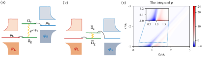
Figure 4: The energy level (a) of the two superconducting leads connected by a light-controlled quantum dot in Eq. (27) by the unitary transformation $\mathbf{U}(t)$ becomes the effective energy level (b) with the reduced lower level $\bar{\Omega}_{\mathrm{g}}=\Omega_{\mathrm{g}}-\mu_{\mathrm{L}}$and upper level $\bar{\Omega}_{\mathrm{e}}=\Omega_{\mathrm{e}}-\mu_{\mathrm{R}}$, and the phase $\bar{\varphi}_{\mathrm{R}}=\varphi_{\mathrm{R}}+2\phi_{\mathrm{d}}$ of the right superconducting of (38) in the rotation representation. Plotted (c) shows that the main contribution of the integrand $\rho(\nu)$ in Eq. (46) to the integral is concentrated between $-1.2\Delta_{\mathrm{s}}$ and $-\Delta_{\mathrm{s}}$ when the driving strength $\mathcal{E}_{\mathrm{d}}$ changes from $0.3\Delta_{\mathrm{s}}$ to $1.8\Delta_{\mathrm{s}}$, which is shown more clearly in the inset.

Thus, according to Eq. (24, 25), the transport current (24) is zero due to the same chemical potentials of the left and right superconducting lead, and the proximity current (25) induced by the light simplified as

$$I_{\mathrm{s}}=\frac{e}{2\hbar}\int_{-\infty}^{+\infty}\frac{d\nu}{2\pi}\,\text{tr}\{[\mathbf{G}(\nu)-\mathbf{G}^{\dagger}(\nu)][\boldsymbol{\Gamma}_{\mathrm{L}}^{+}(\nu),\mathbf{P}^{+}]_{-}\}f_{\mathrm{L}}(\nu)++\text{tr}\{[\mathbf{G}(\nu)-\mathbf{G}^{\dagger}(\nu)][\boldsymbol{\Gamma}_{\mathrm{L}}^{-}(\nu),\mathbf{P}^{+}]_{-}\}\bar{f}_{\mathrm{L}}(-\nu).$$ (42)

In deriving above current formula, the following relation is needed

$$\mathbf{G}^{\dagger}(\nu)-\mathbf{G}(\nu)=-2i\mathbf{G}(\nu)(\nu-[\mathbf{H}+\sum_{\mathrm{m}}\mathbf{V}_{\mathrm{m}}(\nu)])\mathbf{G}^{\dagger}(\nu).$$ (43)

Together with the Hamiltonian $\mathbf{H}$ of the measured system (39) and the dissipation kernel $\mathbf{D}(\omega)=\sum_{\mathrm{m=L,R}}\mathbf{D}_{\mathrm{m}}(\omega)$ caused by the two superconducting leads in Eq. (20), the Green function $\mathbf{G}(\omega)=i[\omega^{+}-\mathbf{H}+i\mathbf{D}(\omega)]^{-1}$ is obtained. Further, the dc current induced by the light, which is completely driven by the superconducting phase difference $\Phi:=\bar{\varphi}_{\mathrm{R}}-\varphi_{\mathrm{L}}=2\phi_{\mathrm{d}}+\varphi_{\mathrm{R}}-\varphi_{\mathrm{L}}$, are exactly calculated as

$$I_{\mathrm{s}} =\frac{e}{h}\int d\nu\frac{256\Gamma^{3}\Delta_{\mathrm{s}}^{2}\nu^{2}\mathcal{E}_{\mathrm{d}}^{2}\left(\Omega_{\Gamma}^{2}-4\nu^{2}\right)\text{Sgn}[\nu]\Re[\gamma_{\mathrm{s}}(\nu)]f_{\mathrm{L}}(\nu)\sin(\Phi)}{64\Gamma^{2}\nu^{4}\gamma_{\mathrm{s}}^{2}(\nu)(\Omega_{\Gamma}^{2}-4\nu^{2})^{2}+\left(4\Gamma^{2}\left(\Delta_{\mathrm{s}}^{2}\Omega_{\delta}^{2}(\Phi)+\nu^{2}(4\nu^{2}-\Omega^{2})\right)-\gamma_{\mathrm{s}}^{2}(\nu)[(\Gamma^{2}-4\nu^{2})^{2}-16(\nu^{2}\Omega^{2}-\mathcal{E}_{\mathrm{d}}^{4})]\right)^{2}}$$

$$:=I_{c}(\Phi)\sin(\Phi).$$ (44)

Here, we have considered the reduced lower energy for simplicity $\bar{\Omega}_{\mathrm{g}}=\Omega_{\mathrm{g}}-\mu_{\mathrm{L}}\equiv 0$ and the same coupling strength $\Gamma_{\mathrm{L}}=\Gamma_{\mathrm{R}}=\Gamma$, and the light-atom detuning is defined as $\delta\omega=\Omega_{\mathrm{e}}-\Omega_{\mathrm{g}}-\omega_{\mathrm{d}}$. At the same time, the following notations are also used for simplifying the above formula

$$\Omega=\sqrt{\delta\omega^{2}+2\mathcal{E}_{\mathrm{d}}^{2}},\quad\Omega_{\Gamma}=\sqrt{2\Omega^{2}+\Gamma^{2}},\quad\Omega_{\delta}^{2}(\Phi)=\delta\omega^{2}+2\mathcal{E}_{\mathrm{d}}^{2}\cos\Phi,\quad\gamma_{\mathrm{s}}(\nu)=\sqrt{\nu^{2}-\Delta_{\mathrm{s}}^{2}}.$$ (45)

In the large detuning situation ($\delta\omega\gg\mathcal{E}_{\mathrm{d}}$), since $\Omega_{\mathrm{\delta}}^{2}(\Phi)=\delta\omega^{2}+2\mathcal{E}_{\mathrm{d}}^{2}\cos\Phi\simeq\delta\omega^{2}$, the above critical current $I_{c}(\Phi)\simeq I_{c}$ becomes a constant independent of the phase difference $\Phi$, then the above supercurrent (44) is simplified as $I_{\mathrm{s}}=I_{c}\sin\Phi$. And, it can be seen from Eq. (44) that the integrand is given as

$$\rho(\nu)=\frac{\Delta_{\mathrm{s}}^{2}\nu^{2}\mathcal{E}_{\mathrm{d}}^{2}\left(\Omega_{\Gamma}^{2}-4\nu^{2}\right)\text{Sgn}[\nu]\Re[\gamma_{\mathrm{s}}(\nu)]f_{\mathrm{L}}(\nu)}{64\Gamma^{2}\nu^{4}\gamma_{\mathrm{s}}^{2}(\nu)(\Omega_{\Gamma}^{2}-4\nu^{2})^{2}+\left(4\Gamma^{2}\left(\Delta_{\mathrm{s}}^{2}\Omega_{\delta}^{2}(\Phi)+\nu^{2}(4\nu^{2}-\Omega^{2})\right)-\gamma_{\mathrm{s}}^{2}(\nu)[(\Gamma^{2}-4\nu^{2})^{2}-16(\nu^{2}\Omega^{2}-\mathcal{E}_{\mathrm{d}}^{4})]\right)^{2}},$$ (46)

the main contribution of which to the integral comes from near $\nu\sim-\Delta_{\mathrm{s}}$ due to $\left(\nu^{2}-\Delta_{\mathrm{s}}^{2}\right)^{-\frac{1}{2}}\rightarrow\infty$ when $\nu\rightarrow-\Delta_{\mathrm{s}}-\varepsilon$ ($\varepsilon$ is infinitesimal), which can be proved exactly by numerical computation, as shown in Fig. 4 (c).

Appendix C The supercurrent through SQUID with two quantum dots

In this section, we consider that the two same QDs embedded in a superconducting quantum interference devices (SQUID) loop is driven by the coherence of light. According to the Hamiltonian of the QD coupled by the light in Eqs (28, 29), the two QDs coupled through the coherence light is described by

$$H_{s}=\sum_{i=1,2}[\Omega_{\mathrm{e}}\sum_{\sigma}d_{i,\mathrm{e}\sigma}^{\dagger}d_{i,\mathrm{e}\sigma}+\Omega_{\mathrm{g}}\sum_{\sigma}d_{i,\mathrm{g}\sigma}^{\dagger}d_{i,\mathrm{g}\sigma}-\mathcal{E}_{i,\mathrm{d}}d_{i,\mathrm{e}\sigma}^{\dagger}d_{i,\mathrm{g}\sigma}e^{-i\omega_{\mathrm{d}}t-i\phi_{i,\mathrm{d}}}-\mathcal{E}_{i,\mathrm{d}}d_{i,\mathrm{g}\sigma}^{\dagger}d_{i,\mathrm{e}\sigma}e^{i\omega_{\mathrm{d}}t+i\phi_{i,\mathrm{d}}}].$$ (47)

Here, we have considered the same the frequency of the driving light $\omega_{\mathrm{d},1}=\omega_{\mathrm{d},2}=\omega_{\mathrm{d}}.$ Similarly, the tunneling interaction between QD and the superconducting leads under the rotating wave approximation are rewritten as

$$\hat{H}_{t}=-\sum_{i=1,2}\sum_{\mathbf{k},\sigma}[\mathrm{t}_{\mathrm{R},\mathrm{e},\mathbf{k}}d_{i,\mathrm{e}\sigma}^{\dagger}c_{\mathrm{R},\mathbf{k}\sigma}+\mathrm{t}_{\mathrm{L},\mathrm{g},\mathbf{k}}d_{i,\mathrm{g}\sigma}^{\dagger}c_{\mathrm{L},\mathbf{k}\sigma}+\mathrm{H.c.}].$$ (48)

In the case where the light frequency is equal to the difference of chemical potential between two superconducting leads, i.e. $\omega_{\mathrm{d}}=\mu_{\mathrm{R}}-\mu_{\mathrm{L}}$, we can introduce unitary transform

$$\mathbf{U}(t)=\exp[i(N_{\mathrm{L}}+\sum_{i\sigma}d_{i,\mathrm{g}\sigma}^{\dagger}d_{i,\mathrm{g}\sigma})\mu_{\mathrm{L}}t+i(N_{\mathrm{R}}+\sum_{i\sigma}d_{i,\mathrm{e}\sigma}^{\dagger}d_{i,\mathrm{e}\sigma})\mu_{\mathrm{R}}t+i\sum_{i\sigma}d_{i,\mathrm{e}\sigma}^{\dagger}d_{i,\mathrm{e}\sigma})\phi_{i,\mathrm{d}}],$$ (49)

to obtain the transformed Hamiltonian: $\bar{H}_{s}=\frac{1}{2}\mathbf{d}^{\dagger}\cdot\mathbf{H}\cdot\mathbf{d}$, where the Hamiltonian matrix in vector operator basis $\mathbf{d}=[\mathsf{d}_{1,\mathrm{e}},\mathsf{d}_{1,\mathrm{g}},\mathsf{d}_{2,\mathrm{e}},\mathsf{d}_{2,\mathrm{g}}]^{T}$ is $\mathbf{H}=\mathrm{diag}\{\mathbf{H}_{Q,1},\mathbf{H}_{Q,2}\}$ with the block matrix $\mathbf{H}_{Q,i}$ defined in Eq. (39). Respectively, by defining the vector operator of the right superconducting lead

$$\bar{\mathbf{c}}_{i,\mathrm{R},\mathbf{k}}=[\bar{c}_{i,\mathrm{R},\mathbf{k}\uparrow},\bar{c}_{i,\mathrm{R},-\mathbf{k}\downarrow},\bar{c}_{i,\mathrm{R},\mathbf{k}\uparrow}^{\dagger},\bar{c}_{i,\mathrm{R},-\mathbf{k}\downarrow}^{\dagger}]^{T}\equiv[e^{i\phi_{i,\mathrm{d}}}c_{\mathrm{R},\mathbf{k}\uparrow},e^{i\phi_{i,\mathrm{d}}}c_{\mathrm{R},-\mathbf{k}\downarrow},e^{-i\phi_{i,\mathrm{d}}}c_{\mathrm{R},\mathbf{k}\uparrow}^{\dagger},e^{-i\phi_{i,\mathrm{d}}}c_{\mathrm{R},-\mathbf{k}\downarrow}^{\dagger}]^{T},$$ (50)

we can obtain the tunneling Hamiltonian between QD and the superconducting leads

$$H_{t}=-\sum_{i=1,2}\sum_{\mathbf{k},\sigma}[\mathrm{t}_{\mathrm{R},\mathrm{e},\mathbf{k}}d_{i,\mathrm{e}\sigma}^{\dagger}\bar{c}_{i,\mathrm{R},\mathbf{k}\sigma}+\mathrm{t}_{\mathrm{L},\mathrm{g},\mathbf{k}}d_{i,\mathrm{g}\sigma}^{\dagger}c_{\mathrm{L},\mathbf{k}\sigma}+\mathrm{H.c.}].$$ (51)

and the Hamiltonian of the superconducting lead-$\mathrm{n}$:

$$\bar{H}_{i,\mathrm{n}}^{\mathrm{s}} =\frac{1}{2}\bar{\mathbf{c}}_{i,\mathrm{n},\mathbf{k}}^{\dagger}\cdot\mathbf{H}_{i,\mathrm{n}}\cdot\bar{\mathbf{c}}_{i,\mathrm{n},\mathbf{k}}\equiv\frac{1}{2}\bar{\mathbf{c}}_{i,\mathrm{n},\mathbf{k}}^{\dagger}\cdot\begin{bmatrix}\epsilon_{\mathrm{n},\mathbf{k}}&&&\Delta_{i,\mathrm{n}}\\ &\epsilon_{\mathrm{n},\mathbf{k}}&-\Delta_{i,\mathrm{n}}\\ &-\Delta_{i,\alpha}^{*}&-\epsilon_{\mathrm{n},\mathbf{k}}\\ \Delta_{i,\mathrm{n}}^{*}&&&-\epsilon_{\mathrm{n},\mathbf{k}}\end{bmatrix}\cdot\bar{\mathbf{c}}_{i,\mathrm{n},\mathbf{k}},\>\mathrm{n}=\mathrm{L,R},$$ (52)

where the pairing term of the left and right superconducting lead are $\Delta_{i,\mathrm{L}}=\Delta_{\mathrm{s}}e^{i\varphi_{\mathrm{L}}}$ and $\Delta_{i,\mathrm{R}}=\Delta_{\mathrm{s}}e^{i(\varphi_{\mathrm{R}}+2\phi_{i,\mathrm{d}})}$.

As the block diagonal Hamiltonian $\mathbf{H}=\mathrm{diag}\{\mathbf{H}_{Q,1},\mathbf{H}_{Q,2}\}$ of the measured system and the dissipation kenal $\mathbf{D}(\omega)=\sum_{\mathrm{m=L,R}}\mathbf{D}_{\mathrm{m}}(\omega)$ in Eq. (20) are block diagonal, the Green function $\mathbf{G}(\omega)=i[\omega^{+}-\mathbf{H}+i\mathbf{D}(\omega)]^{-1}$ is also rewritten as $8\times 8$ block diagonal matrix. Therefore, also using Eq. (42), the total current is the sum of the current flowing through two QDs respectively

$$I_{\mathrm{s}}=I_{\mathrm{s},1}+I_{\mathrm{s},2}$$ (53)

Here, the current through each quantum dot is $I_{\mathrm{s},i}=I_{c,i}(\Phi_{i})\sin\Phi_{i}$ with total phase $\Phi_{1}=\varphi_{\mathrm{R}}-\varphi_{\mathrm{L}}+2\phi_{1,\mathrm{d}}$ and $\Phi_{2}=\varphi_{\mathrm{R}}-\varphi_{\mathrm{L}}+2\phi_{2,\mathrm{d}}$, which is given in Eq. (44).