WSFE: Wasserstein Sub-graph Feature Encoder for Effective User Segmentation in Collaborative Filtering

Abstract.

Maximizing the user-item engagement based on vectorized embeddings is a standard procedure of recent recommender models. Despite the superior performance for item recommendations, these methods however implicitly deprioritize the modeling of user-wise similarity in the embedding space; consequently, identifying similar users is underperforming, and additional processing schemes are usually required otherwise. To avoid thorough model re-training, we propose WSFE, a model-agnostic and training-free representation encoder, to be flexibly employed on the fly for effective user segmentation. Underpinned by the optimal transport theory, the encoded representations from WSFE  present a matched user-wise similarity/distance measurement between the realistic and embedding space. We incorporate WSFE  into six state-of-the-art recommender models and conduct extensive experiments on six real-world datasets. The empirical analyses well demonstrate the superiority and generality of WSFE to fuel multiple downstream tasks with diverse underlying targets in recommendation.

1. Introduction

Collaborative filtering (CF), as one effective strategy to perform personalized modeling and prediction, has been widely deployed for recommendation. One prevalent learning paradigm of CF models (He et al., 2020; Ying et al., 2018; Ling et al., 2012; Chen et al., 2022a; Yang et al., 2022a; Wu et al., 2020) is to parameterize users and items as vectorized embeddings and learn to reconstruct users’ historical interactions. As such, the learned embeddings are convenient to interpret target users’ diverse preferences and predict their future behaviors.

In addition to reflecting preferences on items, another desirable property of learned user embeddings is to explicitly capture the user-wise similarity; this provides an intuitive recognition of similar user interests and affinities, which lays the foundation and is particularly beneficial for user-centric analyses and applications such as group recommendation and advertising (Shen et al., 2023b, d). However, this property is usually deprioritized and neglected by recent models (He et al., 2020; Wang et al., 2019; Wu et al., 2021; Lee et al., 2021; Yang et al., 2022b; Luo et al., 2022). To address the unsatisfactory performance in similar user identification, thorough model re-training may thus be required. To tackle this issue, we are motivated to encode high-quality embeddings in collaborative filtering, such that they can efficiently and seamlessly serve the task of user segmentation.

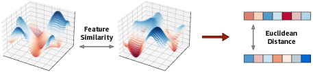
Figure 1. Illustration of WSFE  in encoding the similarity of empirical feature distribution (left) with the corresponding embedding distance (right).

In this work, we propose Wasserstein Sub-graph Feature Encoder (WSFE), to explicitly model the user behaviors in the form of user-item interaction graph, and measure the user-wise similarity by exploiting their high-order sub-graph patterns. We notice that users with similar interaction behaviors naturally share overlapping sub-graph patterns. Based on this observation, one straightforward solution would be to exhaustively calculate similarities for all the nodes in underlying sub-graphs; this however may be intractable in practice mainly because of the exponential node scale in graph exploration. On the contrary, our proposed WSFE captures user similarity by directly encoding their sub-graph latent features, enabling it model-agnostic and flexible for a variety of graph-based recommender models. Specifically, as shown in Figure 1, we assume the user preference follows an unknown high-dimensional probability distribution; this unique preference distribution is empirically observed and represented by the latent features that are well-learned in the item recommendation task. Then WSFE explicitly captures the distribution distances with Wasserstein metrics from the optimal transport theory (Rabin et al., 2011; Villani, 2009; Naderializadeh et al., 2021; Kolouri et al., 2020). Consequently, the encoded user representations can effectively reflect their realistic item-interaction similarity, producing a matched Euclidean distance measurement for ease of user segmentation in the embedding space.

To summarize, our contributions are highlighted as follows:

• To the best of our knowledge, we are the first to focus on improving the embedding quality for effective user segmentation in collaborative filtering, while not jeopardizing the model evaluation for item recommendation.

• We propose WSFE for effective representation encoding via capturing the feature similarity of high-order user-item interaction graph patterns. WSFE  is adaptive for any graph-based models and training-free; thus it can be invoked on the fly as long as the backbone models are well-trained.

• We conduct extensive experiments by fusing WSFE into six state-of-the-art models on six real-world datasets. Not only do we present its performance superiority in empirical evaluation, but we also provide technical discussion for future investigation.

2. WSFE Methodology

2.1. Preliminaries

Graph-based Collaborative Filtering. In view of user-item interaction graphs, the general idea of graph-based approaches is to capture CF signals in high-hop neighbors. In this work, we study the Graph Convolutional Networks (GCNs) to learn node representations by smoothing the latent features via topology (Kipf and Welling, 2017; Chen et al., 2023; Song et al., 2022, 2021). It iteratively propagates neighborhood information to the target node, e.g., user $u$, which can be abstracted:

(1) $$\boldsymbol{v}_{ngh\rightarrow u}^{(l)}=Prop\Big{(}\{\boldsymbol{v}_{i}^{(l-1)}:i\in\mathcal{N}(u)\}\Big{)},$$

where $\boldsymbol{v}_{ngh\rightarrow u}^{(l)}$ is the representation after $l$ layers of propagation from interacted items in $u$’s neighboring set $\mathcal{N}(u)$. With the propagated information, node embeddings are iteratively updated by aggregating features of the center and neighbor nodes (Hamilton et al., 2017; Zhang et al., 2022a; He et al., 2023).

Optimal Transport and Wasserstein Metrics. Optimal transport is the general problem of moving one distribution of mass, e.g., $P$, to another, e.g., $Q$, as efficiently as possible. The derived minimum $L_{2}$ cost can be referred as their distribution distance:

(2) $$W_{2}(P,Q)=\Big{(}{\inf}_{f\in\mathcal{F}(P,Q)}\int\|\boldsymbol{x}-f(\boldsymbol{x})\|^{2}dP(\boldsymbol{x})\Big{)}^{\frac{1}{2}},$$

where the infimum is over all transport plans in $\mathcal{F}$ between $P$ and $Q$. For one-dimensional distributions, there is a closed-form solution to compute such optimal transport map $f^{*}$ as $f^{*}(x):=F_{P}^{-1}\big{(}F_{Q}(x)\big{)}$; $F$ is the cumulative distribution function (CDF) associated with $P$.

For the high-dimensional case, the metric of sliced-Wasserstein distance (Rabin et al., 2011; Bonneel et al., 2015; Deshpande et al., 2019) is formally defined as follows:

(3) $$SW_{2}\left(P,Q\right)=\Big{(}\int_{\mathbb{S}^{d-1}}W_{2}^{2}\big{(}P^{\boldsymbol{\theta}},Q^{\boldsymbol{\theta}}\big{)}d\small{\boldsymbol{\theta}}\Big{)}^{\frac{1}{2}},$$

where $P^{\boldsymbol{\theta}}$ is projected by function $g^{\boldsymbol{\theta}}$: $\mathbb{R}^{d}$ $\rightarrow$ $\mathbb{R}$ as $P^{\boldsymbol{\theta}}$ := $g^{\boldsymbol{\theta}}(P)$ and $g^{\boldsymbol{\theta}}(\small{x})={\small{\boldsymbol{\theta}}^{\mathsf{T}}x}$. ${\small\boldsymbol{\theta}}$ is a unit vector in $\mathbb{R}^{d}$ and $\mathbb{S}^{d-1}$ is the unit $d$-dimensional hypersphere. Due to holding positive-definiteness, symmetry, and triangle inequality (Kolouri et al., 2016, 2019; Naderializadeh et al., 2021; Zhang and Zhu, 2020; Shen et al., 2023a), we employ it as the distance measurement for high-dimensional subgraph feature distributions.

2.2. Sub-graph Feature Encoding

2.2.1. Formulating Sub-graph Feature Distributions.

As illustrated in Figure 2(A), if two users are considered to be similar in terms of historical preferences, they should share similar behaviors with overlapping interaction graph patterns. Based on this intuition, consider that each user’s preference follows an unknown, independent, and $d$-dimensional probability measure, e.g., $P_{u}$. We assume that the interaction pattern of $u$ observed so far is sampled from the underlying distribution $P_{u}$. Thus the empirical (discrete) distribution $\widehat{P}_{u}$ with its empirical CDF can be formulated as:

(4) $$F_{\widehat{P}_{u}}(\boldsymbol{x})=\frac{1}{L+1}{\sum}_{l=0}^{L}\delta(\boldsymbol{x}-\boldsymbol{v}_{ngh\rightarrow u}^{(l)}).$$

Notice that we initialize $\boldsymbol{v}_{ngh\rightarrow u}^{(0)}$ $:=$ $\boldsymbol{v}_{u}^{(0)}$. Here $\delta(\cdot)$ returns 1 if the input is zero and 0 otherwise (discretizing from continuous case $\int$$\delta(x)dx$ $=$ $1$). Without loss of generality, these empirical distributions are representative, i.e., $\widehat{P}_{u}$ $\approx$ $P_{u}$; thus we would refer $P_{u}$ to $\widehat{P}_{u}$ hereafter to avoid notation abuse.

2.2.2. Implementing $f^{*}$.

We first set a $d$-dimensional reference distribution $P_{o}$ that functions as the “origin” in the embedding space to measure the distance toward any inputs. $P_{o}$ is associated with random feature embeddings, e.g., $\boldsymbol{v}_{o}^{(l)}$, as: $F_{{P}_{o}}(\boldsymbol{x})=\frac{1}{L+1}{\sum}_{n=0}^{L}\delta(\boldsymbol{x}-\boldsymbol{v}_{o}^{(l)})$. To implement the optimal transport map $f^{*}$ for such discrete and $d$-dimensional case, we have the following procedure.

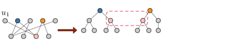
Figure 2. (A) Illustration of the similar sub-graph patterns. (B) Mapping processing between the input and reference.

We first conduct distribution slicing to $P_{o}$ and $P_{u}$ by projection function $g^{\boldsymbol{\theta}}$. For each pair of distribution slices $P_{u}^{\boldsymbol{\theta}}$ and $P_{o}^{\boldsymbol{\theta}}$, let $\mathcal{X}_{u}^{\boldsymbol{\theta}}$ collect their projected sub-graph features as $\mathcal{X}_{u}^{\boldsymbol{\theta}}$ = $\{\boldsymbol{\theta}^{\mathsf{T}}\boldsymbol{v}_{ngh\rightarrow u}^{(l)}\}_{l=0}^{L}$ (so does for $\mathcal{X}_{o}^{\boldsymbol{\theta}}$ = $\{\boldsymbol{\theta}^{\mathsf{T}}\boldsymbol{v}_{o}^{(l)}\}_{l=0}^{L}$). Then the corresponding optimal transport map $f^{*}(x):=F_{P_{u}^{\boldsymbol{\theta}}}^{-1}\big{(}F_{P_{o}^{\boldsymbol{\theta}}}(x)\big{)}$ can be quantitatively intepreted:

(5) $${f}^{*}(x|\mathcal{X}_{u}^{\boldsymbol{\theta}})=\operatorname{argmin}_{x^{\prime}\in\mathcal{X}_{u}^{\boldsymbol{\theta}}}\big{(}F_{P_{u}^{\boldsymbol{\theta}}}(x^{\prime})=r\big{)}\text{, where }r=F_{P_{o}^{\boldsymbol{\theta}}}(x).$$

Furthermore, let $\tau(x^{\prime}|\mathcal{X}_{u}^{\boldsymbol{\theta}})$ denote the ranking of each input $x^{\prime}$ in the ascending sorting of $\mathcal{X}_{u}^{\boldsymbol{\theta}}$. We can replace the term $F_{P_{u}^{\boldsymbol{\theta}}}$ and have:

(6) $$f^{*}(x|\mathcal{X}_{u}^{\boldsymbol{\theta}})=\operatorname{argmin}_{x^{\prime}\in\mathcal{X}_{u}^{\boldsymbol{\theta}}}\big{(}\tau(x^{\prime}|\mathcal{X}_{u}^{\boldsymbol{\theta}})=\tau(x|\mathcal{X}_{o}^{\boldsymbol{\theta}})\big{)}.$$

As shown in Figure 2(B), Eqn.(6) essentially permutes different layers of sub-graph embeddings of $\mathcal{X}_{u}^{\boldsymbol{\theta}}$ in encoding, such that the distance to the reference of $\mathcal{X}_{o}^{\boldsymbol{\theta}}$ can be subsequently captured and embedded. Please notice that the distance is in the $L_{2}$-norm form as shown in Eqn.(2), a.k.a. the Euclidean distance, which is favorable to scenarios for recalling vectorized objects that requires a reasonable distance measurement in the embedding space.

2.2.3. Implementing WSFE.

For each pair of distribution slices, based on the algorithmic implementation of Eqn.(6), we proceed to encode their representations as follows:

(7) $$\boldsymbol{E}_{u}^{\boldsymbol{\theta}}:=\frac{1}{L+1}\Big{\|}_{l=0}^{L}f^{*}\Big{(}{\boldsymbol{\theta}}^{\mathsf{T}}\boldsymbol{v}_{o}^{(l)}|\mathcal{X}_{u}^{\boldsymbol{\theta}}\Big{)}-\boldsymbol{E}_{o}^{\boldsymbol{\theta}}\text{ and }\boldsymbol{E}_{o}^{\boldsymbol{\theta}}:=\frac{1}{L+1}\Big{\|}_{l=0}^{L}{\boldsymbol{\theta}}^{\mathsf{T}}\boldsymbol{v}_{o}^{(l)},$$

where $||$ denotes the concatenation operation. According to the theory in Eqn.(3), the next step is to draw infinite projections for distance integral, which, however, may be computationally expensive and infeasible in practice. In this work, we implement it with Monte-Carlo approximation with $S$ times of uniform sampling from $\mathbb{S}^{d-1}$. Consequently, this leads to a cumulative sliced-Wasserstein distance (i.e., approximating Eqn.(3)) between reference $P_{o}$ and the original input feature distribution $P_{u}$ as:

(8) $$SW_{2}(P_{o},P_{u})\approx\Big{(}\frac{1}{S}{\sum}_{s=1}^{S}W_{2}^{2}\big{(}P_{o}^{\theta_{s}},P_{u}^{\theta_{s}}\big{)}\Big{)}^{\frac{1}{2}}.$$

Regularized by the distance cumulation in Eqn.(8), our Wasserstein Sub-graph Feature Encoder (WSFE) is finally defined:

(9) $$\boldsymbol{E}_{u}:=\frac{1}{S}\Big{\|}_{s=1}^{S}\boldsymbol{E}_{u}^{\boldsymbol{\theta}_{s}}\text{ \quad and \quad}\boldsymbol{E}_{o}:=\frac{1}{S}\Big{\|}_{s=1}^{S}\boldsymbol{E}_{o}^{\boldsymbol{\theta}_{s}},$$

where $\boldsymbol{E}_{u}$, $\boldsymbol{E}_{o}$ $\in$ $\mathbb{R}^{S(L+1)}$. Notice that in practice, the number of graph convolutions $L$ $\leq$ 4 (He et al., 2020; Kipf and Welling, 2017; Hamilton et al., 2017) is a common setting mainly to avoid the over-smoothing problem (Li et al., 2019). Moreover, our empirical observations in § 3.2.2 reveal that setting $S=64$ already achieves satisfactory model performances with an acceptable computational cost.

2.3. Theoretical Analysis

One major expectation of encoded representations is that they can reflect the similarity/distance of their sub-graph feature distributions. We illustrate this in Figure 3 with the theorem as follows:

Theorem 1. For any input sub-graph features of users $u_{i}$ and $u_{j}$ with distributions $P_{u_{i}}$ and $P_{u_{j}}$, their encoded representations hold:

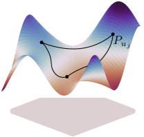
Figure 3. Wasserstein to Euclidean geodesics.

\raisebox{-0.7pt}{1}⃝ $\|\boldsymbol{E}_{u_{i}}\|_{2}$ $\approx$ $SW_{2}(P_{u_{i}},P_{0})$.
\raisebox{-0.7pt}{2}⃝ $\|\boldsymbol{E}_{u_{i}}-\boldsymbol{E}_{u_{j}}\|_{2}$ $\approx$ $SW_{2}(P_{u_{i}},P_{u_{j}})$.

Proof. The proof is twofold. For property \raisebox{-0.7pt}{2}⃝, we have:

(10) $$\quad\|\boldsymbol{E}_{u_{i}}-\boldsymbol{E}_{u_{j}}\|_{2}$$

$$=\Big{\|}\big{\|}_{s=1}^{S}(\boldsymbol{E}_{u_{i}}^{\boldsymbol{\theta}_{s}}-\boldsymbol{E}_{u_{j}}^{\boldsymbol{\theta}_{s}})\Big{\|}_{2}$$

$$=\Big{\|}{\sum}_{s=1}^{S}(\boldsymbol{E}_{u_{i}}^{\boldsymbol{\theta}_{s}}-\boldsymbol{E}_{u_{j}}^{\boldsymbol{\theta}_{s}})^{2}\Big{\|}_{2}$$

$$=\Big{\|}\frac{1}{S}{{\sum}}_{s=1}^{S}\frac{1}{L+1}{\sum}_{l=0}^{L}\left({f^{*}}(\boldsymbol{\theta}_{s}^{\mathsf{T}}\boldsymbol{v}^{(l)}_{o}|\mathcal{X}_{{u_{i}}}^{\boldsymbol{\theta}_{s}})-{f^{*}}(\boldsymbol{\theta}_{s}^{\mathsf{T}}\boldsymbol{v}^{(l)}_{o}|\mathcal{X}_{u_{j}}^{\boldsymbol{\theta}_{s}})\right)^{2}\Big{\|}_{2}$$

$$\approx\Big{\|}\int_{\mathbb{S}^{d-1}}\int_{\mathbb{R}}\Big{(}F^{-1}_{P_{u_{i}}^{\boldsymbol{\theta}}}\big{(}F_{P_{o}^{\boldsymbol{\theta}}}(t)\big{)}-F^{-1}_{P_{u_{j}}^{\boldsymbol{\theta}}}\big{(}F_{P_{o}^{\boldsymbol{\theta}}}(t)\big{)}\Big{)}^{2}dP_{o}^{\boldsymbol{\theta}}(t)d{\boldsymbol{\theta}}\Big{\|}_{2}$$

$$=\Big{\|}\int_{\mathbb{S}^{d-1}}\int_{0}^{1}\big{(}F_{P_{u_{i}}^{\boldsymbol{\theta}}}^{-1}(r)-F_{P_{u_{j}}^{\boldsymbol{\theta}}}^{-1}(r)\big{)}^{2}drd{\boldsymbol{\theta}}\Big{\|}_{2}.$$

Let $F^{-1}_{P_{u_{i}}^{\boldsymbol{\theta}}}(r)$ = $x$, meaning that $r$ = $F_{P_{u_{i}}^{\boldsymbol{\theta}}}$. We have:

(11) $$\quad\|\boldsymbol{E}_{u_{i}}-\boldsymbol{E}_{u_{j}}\|_{2} =\Big{\|}\int_{\mathbb{S}^{d-1}}\int_{0}^{1}\big{(}x-F_{P_{u_{j}}^{\boldsymbol{\theta}}}^{-1}(F_{P_{u_{i}}^{\boldsymbol{\theta}}}(x))\big{)}^{2}dP_{u_{j}}^{\theta}(x)d{\boldsymbol{\theta}}\Big{\|}_{2}$$

$$=\Big{\|}\int_{\mathbb{S}^{d-1}}W_{2}^{2}(P_{u_{j}}^{\boldsymbol{\theta}},P_{u_{i}}^{\boldsymbol{\theta}})d{\boldsymbol{\theta}}\Big{\|}_{2}=SW_{2}(P_{u_{j}},P_{u_{i}}).$$

With symmetry, we have $SW_{2}(P_{u_{i}},P_{u_{j}})$ = $SW_{2}(P_{u_{j}},P_{u_{i}})$. Then for the reference $P_{o}$, its encoded representation is straightforward to have $\boldsymbol{E}_{o}$ = $\boldsymbol{0}$. Thus we complete the proof as follows:

(12) $$\|\boldsymbol{E}_{u_{i}}\|_{2}=\|\boldsymbol{E}_{u_{i}}-\boldsymbol{E}_{o}\|_{2}\approx SW_{2}(P_{u_{i}},P_{o}),$$

$\hfill\blacksquare$

Complexity Analysis. WSFE is training-free that can be utilized on the fly right after the backbone model is trained. Thus, the complexity of WSFE  is $O\big{(}S(L+1)M{d}\log{d}\big{)}$, where the cost $O(d\log{d})$ is for implementing $\tau(\cdot)$. Fortunately, it is linear to the input data size, indicating that the encoding can be done at the input scale.

3. Experimental Results

We evaluate WSFE with the aim of answering the following research questions: RQ1. How does WSFE  boost the user segmentation performance of state-of-the-art recommender models? RQ2. How do different model settings affect WSFE  performance?

3.1. Experimental Setups

Datasets. We collect six widely-evaluated public datasets (including their original training/test data splits) from: MovieLens (MovieLens, 2003; Chen et al., 2022c, b; Zhang et al., 2022a), Gowalla (Cho et al., 2011; Gowalla, 2011), Pinterest (Geng et al., 2015; Pinterest, 2015), Yelp (Yelp2018, 2018), Kindle (Kindle, 2015; Yu et al., 2022b), and Amazon-Book (Amazon, 2015; He et al., 2020). Dataset statistics are reported in Table 1.

Table 1. The statistics of datasets.

	MovieLens	Gowalla	Pinterest	Yelp2018	Kindle	AMZ-Book
#Users	6,040	29,858	55,186	31,668	115,652	52,643
#Items	3,952	40,981	9,916	38,048	98,729	91,599
#Avg. Interactions	165.60	34.31	26.52	49.31	15.85	56.69
#All Interactions	1,000,209	1,027,370	1,463,556	1,561,406	1,833,068	2,984,108

Evaluation Protocol. The fundamental property required by user segmentation is user-wise similarity measurement. Thus, given a query user, we treat this task as ranking towards candidates of similar users, based on the encoded user representations. In this work, we sort out similar users based on the number of overlapping items they have interacted with; then we compared these ranking lists with Top-K results inferred from the learning models. Recall@K and NDCG@K are the evaluation metrics.

Baselines. To demonstrate the effectiveness of WSFE, we incorporate it into the following state-of-the-art models.

1. LightGCN (He et al., 2020) is one state-of-the-art GCN-based recommender model with a more concise and powerful structure.

2. SGL (Wu et al., 2021) is one representative graph-based model with contrastive learning to tackle the data sparsity issue.

3. SimGCL (Yu et al., 2022a) is the state-of-the-art contrastive-learning-based recommender model that conducts the simplified augmentation directly in the feature space.

4. NCL (Lin et al., 2022) is one of the state-of-the-art graph-based models with contrastive neighborhood information enrichment.

5. BUIR (Lee et al., 2021) is one state-of-the-art model that bootstraps user and item representations for collaborative filtering.

6. DirectAU (Wang et al., 2022) is the latest model that improves the representation quality from the perspective of alignment and uniformity.

3.2. Empirical Analyses and Discussions

3.2.1. Overall Performance (RQ1).

Table 2. Experimental results before and after implementing WSFE  into the underlying models (best view in color).

Dataset	Model	Recall@5	NDCG@5	Recall@20	NDCG@20	Recall@50	NDCG@50	Recall@100	NDCG@100
Movie	LightGCN	0.10$\rightarrow$0.18 ( +80.00%)	0.36$\rightarrow$0.61 ( +69.44%)	0.37$\rightarrow$0.69 ( +86.49%)	0.36$\rightarrow$0.65 ( +80.56%)	0.85$\rightarrow$1.68 ( +97.65%)	0.62$\rightarrow$1.20 ( +93.55%)	1.63$\rightarrow$3.04 ( +86.50%)	0.97$\rightarrow$1.83 ( +88.66%)
	SGL	0.08$\rightarrow$0.13 ( +62.50%)	0.32$\rightarrow$0.47 ( +46.88%)	0.24$\rightarrow$0.37 ( +54.17%)	0.25$\rightarrow$0.39 ( +56.00%)	0.42$\rightarrow$0.73 ( +73.81%)	0.36$\rightarrow$0.59 ( +63.89%)	0.60$\rightarrow$1.22 ( +103.33%)	0.47$\rightarrow$0.81 ( +72.34%)
	SimGCL	0.90$\rightarrow$1.02 ( +13.33%)	3.40$\rightarrow$3.04 ( +13.82%)	2.13$\rightarrow$3.77 ( +77.00%)	2.30$\rightarrow$3.60 ( +56.52%)	3.10$\rightarrow$8.56 ( +176.13%)	2.92$\rightarrow$5.99 ( +105.14%)	4.45$\rightarrow$13.71 ( +208.09%)	3.35$\rightarrow$8.58 ( +156.12%)
	NCL	0.25$\rightarrow$0.38 ( +52.00%)	0.84$\rightarrow$1.30 ( +54.76%)	0.88$\rightarrow$1.47 ( +67.05%)	0.84$\rightarrow$1.38 ( +64.29%)	2.01$\rightarrow$3.42 ( +70.15%)	1.47$\rightarrow$2.47 ( +68.03%)	3.60$\rightarrow$6.19 ( +71.94%)	2.20$\rightarrow$3.74 ( +70.00%)
	BUIR	0.22$\rightarrow$0.24 ( +9.09%)	0.74$\rightarrow$0.82 ( +10.82%)	0.83$\rightarrow$0.96 ( +15.66%)	0.79$\rightarrow$0.92 ( +16.46%)	1.81$\rightarrow$2.19 ( +20.99%)	1.34$\rightarrow$1.60 ( +19.40%)	3.21$\rightarrow$3.95 ( +23.05%)	1.98$\rightarrow$2.40 ( +21.21%)
	DirectAU	0.09$\rightarrow$0.10 ( +11.11%)	0.32$\rightarrow$0.36 ( +12.50%)	0.25$\rightarrow$0.31 ( +24.00%)	0.26$\rightarrow$0.32 ( +23.08%)	0.53$\rightarrow$0.66 ( +24.53%)	0.41$\rightarrow$0.51 ( +24.39%)	0.98$\rightarrow$1.23 ( +25.51%)	0.62$\rightarrow$0.77 ( +24.19%)
Gowalla	LightGCN	4.41$\rightarrow$4.56 ( +3.40%)	6.59$\rightarrow$6.52 (-1.06%)	8.75$\rightarrow$9.26 ( +5.83%)	6.64$\rightarrow$6.80 ( +2.41%)	13.30$\rightarrow$14.05 ( +5.64%)	8.46$\rightarrow$8.71 ( +2.96%)	17.78$\rightarrow$18.86 ( +6.07%)	9.94$\rightarrow$10.29 ( +3.52%)
	SGL	4.96$\rightarrow$5.30 ( +6.85%)	7.58$\rightarrow$7.62 ( +0.53%)	9.85$\rightarrow$10.66 ( +8.22%)	7.53$\rightarrow$7.86 ( +4.38%)	15.13$\rightarrow$16.68 ( +10.24%)	9.66$\rightarrow$10.23 ( +5.90%)	20.70$\rightarrow$22.72 ( +9.76%)	11.49$\rightarrow$12.19 ( +6.09%)
	SimGCL	5.25$\rightarrow$6.94 ( +32.19%)	8.55$\rightarrow$10.32 ( +20.70%)	10.14$\rightarrow$13.99 ( +37.97%)	8.11$\rightarrow$10.52 ( +29.72%)	14.73$\rightarrow$20.23 ( +37.34%)	9.99$\rightarrow$13.02 ( +30.33%)	17.88$\rightarrow$24.15 ( +35.07%)	11.12$\rightarrow$14.34 ( +28.96%)
	NCL	4.65$\rightarrow$5.01 ( +7.53%)	8.31$\rightarrow$8.71 ( +4.81%)	9.41$\rightarrow$10.20 ( +8.40%)	7.81$\rightarrow$8.34 ( +6.79%)	13.78$\rightarrow$15.11 ( +9.65%)	9.71$\rightarrow$10.43 ( +7.42%)	18.16$\rightarrow$20.02 ( +10.24%)	11.22$\rightarrow$12.11 ( +7.93%)
	BUIR	2.94$\rightarrow$3.07 ( +4.42%)	5.64$\rightarrow$5.74 ( +1.77%)	6.65$\rightarrow$6.92 ( +4.06%)	5.52$\rightarrow$5.66 ( +2.54%)	10.74$\rightarrow$11.00 ( +2.42%)	7.30$\rightarrow$7.42 ( +1.64%)	15.09$\rightarrow$15.36 ( +1.79%)	8.78$\rightarrow$8.91 ( +1.48%)
	DirectAU	5.03$\rightarrow$5.41 ( +7.55%)	7.99$\rightarrow$8.22 ( +2.88%)	10.24$\rightarrow$10.98 ( +7.23%)	7.90$\rightarrow$8.31 ( +5.19%)	15.71$\rightarrow$16.94 ( +7.83%)	10.16$\rightarrow$10.74 ( +5.71%)	21.20$\rightarrow$22.86 ( +7.83%)	12.00$\rightarrow$12.73 ( +6.08%)
Pinterest	LightGCN	2.24$\rightarrow$2.38 ( +6.25%)	4.64$\rightarrow$4.94 ( +6.47%)	7.24$\rightarrow$7.68 ( +6.08%)	5.51$\rightarrow$5.87 ( +6.53%)	13.67$\rightarrow$14.67 ( +7.32%)	8.37$\rightarrow$8.94 ( +6.81%)	21.11$\rightarrow$22.65 ( +7.30%)	11.04$\rightarrow$11.81 ( +6.97%)
	SGL	3.93$\rightarrow$3.92 (-0.25%)	7.58$\rightarrow$7.58 (0%)	11.21$\rightarrow$11.35 ( +1.25%)	8.57$\rightarrow$8.63 ( +0.70%)	19.62$\rightarrow$19.86 ( +1.22%)	12.23$\rightarrow$12.35 ( +0.98%)	28.16$\rightarrow$28.44 ( +0.99%)	15.31$\rightarrow$15.44 ( +0.85%)
	SimGCL	5.04$\rightarrow$8.49 ( +68.45%)	9.28$\rightarrow$14.86 ( +60.13%)	13.56$\rightarrow$21.31 ( +57.15%)	10.33$\rightarrow$16.20 ( +56.82%)	22.70$\rightarrow$32.82 ( +44.58%)	14.31$\rightarrow$21.21 ( +48.22%)	31.68$\rightarrow$41.79 ( +31.91%)	17.54$\rightarrow$24.37 ( +38.94%)
	NCL	4.10$\rightarrow$4.63 ( +12.93%)	8.21$\rightarrow$9.11 ( +10.84%)	11.48$\rightarrow$13.02 ( +13.41%)	8.98$\rightarrow$10.08 ( +12.25%)	19.55$\rightarrow$22.32 ( +14.17%)	12.59$\rightarrow$14.18 ( +12.63%)	27.85$\rightarrow$31.76 ( +14.04%)	15.60$\rightarrow$17.58 ( +12.69%)
	BUIR	1.16$\rightarrow$1.22 ( +5.17%)	2.55$\rightarrow$2.64 ( +3.53%)	4.09$\rightarrow$4.31 ( +5.38%)	3.16$\rightarrow$3.28 ( +3.80%)	8.29$\rightarrow$8.77 ( +5.79%)	5.05$\rightarrow$5.26 ( +4.16%)	13.34$\rightarrow$14.16 ( +6.15%)	6.92$\rightarrow$7.23 ( +4.48%)
	DirectAU	8.03$\rightarrow$9.12 ( +13.57%)	13.34$\rightarrow$14.84 ( +11.24%)	21.32$\rightarrow$24.11 ( +13.09%)	15.40$\rightarrow$17.26 ( +12.08%)	34.53$\rightarrow$38.47 ( +11.47%)	20.93$\rightarrow$23.30 ( +11.32%)	46.73$\rightarrow$51.57 ( +10.36%)	25.21$\rightarrow$27.88 ( +10.59%)
Yelp	LightGCN	2.13$\rightarrow$2.37 ( +11.27%)	1.31$\rightarrow$1.64 ( +25.19%)	2.16$\rightarrow$2.72 ( +25.93%)	1.94$\rightarrow$2.39 ( +23.20%)	4.07$\rightarrow$5.23 ( +28.50%)	2.88$\rightarrow$3.62 ( +25.69%)	6.47$\rightarrow$8.37 ( +29.37%)	3.87$\rightarrow$4.88 ( +26.10%)
	SGL	0.92$\rightarrow$0.97 ( +5.43%)	2.43$\rightarrow$2.50 ( +2.88%)	2.28$\rightarrow$2.57 ( +12.72%)	2.14$\rightarrow$2.33 ( +8.88%)	4.06$\rightarrow$4.67 ( +15.02%)	3.02$\rightarrow$3.36 ( +11.26%)	6.21$\rightarrow$7.18 ( +15.62%)	3.91$\rightarrow$4.38 ( +12.02%)
	SimGCL	1.01$\rightarrow$2.00 ( +98.02%)	2.72$\rightarrow$5.24 ( +92.65%)	2.30$\rightarrow$5.31 ( +130.87%)	2.22$\rightarrow$4.83 ( +117.57%)	3.67$\rightarrow$8.68 ( +136.51%)	2.92$\rightarrow$6.52 ( +123.29%)	4.96$\rightarrow$11.71 ( +136.09%)	3.46$\rightarrow$7.78 ( +124.86%)
	NCL	1.16$\rightarrow$1.41 ( +21.55%)	3.43$\rightarrow$4.06 ( +18.37%)	2.91$\rightarrow$3.65 ( +25.43%)	2.87$\rightarrow$3.52 ( +22.65%)	4.76$\rightarrow$6.13 ( +28.78%)	3.83$\rightarrow$4.79 ( +25.07%)	6.74$\rightarrow$8.88 ( +31.75%)	4.67$\rightarrow$5.91 ( +26.55%)
	BUIR	0.53$\rightarrow$0.53 (+0%)	1.61$\rightarrow$1.62 ( +0.62%)	1.55$\rightarrow$1.58 ( +1.94%)	1.49$\rightarrow$1.51 ( +1.34%)	2.76$\rightarrow$2.84 ( +2.90%)	2.13$\rightarrow$2.17 ( +1.88%)	4.19$\rightarrow$4.33 ( +3.34%)	2.74$\rightarrow$2.79 ( +1.82%)
	DirectAU	1.39$\rightarrow$1.66 ( +19.42%)	3.54$\rightarrow$4.12 ( +16.38%)	3.36$\rightarrow$4.15 ( +23.51%)	3.11$\rightarrow$3.74 ( +20.26%)	5.66$\rightarrow$7.05 ( +24.56%)	4.24$\rightarrow$5.15 ( +21.46%)	8.28$\rightarrow$10.27 ( +24.03%)	5.31$\rightarrow$6.46 ( +21.66%)
Kindle	LightGCN	7.21$\rightarrow$7.26 ( +0.69%)	8.81$\rightarrow$8.56 (-2.84%)	14.88$\rightarrow$15.06 ( +1.21%)	10.26$\rightarrow$10.21 (-0.49%)	19.76$\rightarrow$20.23 ( +2.38%)	12.18$\rightarrow$12.19 ( +0.08%)	23.20$\rightarrow$24.01 ( +3.49%)	13.28$\rightarrow$13.37 ( +0.68%)
	SGL	7.90$\rightarrow$7.94 ( +0.51%)	9.63$\rightarrow$9.33 (-3.12%)	16.93$\rightarrow$17.58 ( +3.84%)	11.53$\rightarrow$11.61 ( +0.69%)	23.32$\rightarrow$24.37 ( +4.50%)	13.99$\rightarrow$14.19 ( +1.43%)	27.87$\rightarrow$29.43 ( +5.60%)	15.41$\rightarrow$15.74 ( +2.14%)
	SimGCL	8.54$\rightarrow$8.80 ( +3.04%)	11.55$\rightarrow$11.25 (-2.60%)	17.27$\rightarrow$18.57 ( +7.53%)	12.62$\rightarrow$12.98 ( +2.85%)	22.79$\rightarrow$24.71 ( +8.42%)	14.82$\rightarrow$15.38 ( +3.78%)	25.95$\rightarrow$28.20 ( +8.67%)	16.87$\rightarrow$17.50 ( +3.73%)
	NCL	9.26$\rightarrow$9.66 ( +4.32%)	12.55$\rightarrow$12.85 ( +2.39%)	18.25$\rightarrow$19.42 ( +6.41%)	13.50$\rightarrow$14.10 ( +4.44%)	23.89$\rightarrow$25.43 ( +6.45%)	15.83$\rightarrow$16.58 ( +4.74%)	27.62$\rightarrow$29.60 ( +7.17%)	17.08$\rightarrow$17.96 ( +5.15%)
	BUIR	7.30$\rightarrow$7.43 ( +1.78%)	10.01$\rightarrow$10.01 (0%)	15.50$\rightarrow$15.67 ( +1.10%)	11.28$\rightarrow$11.34 ( +0.53%)	20.64$\rightarrow$20.98 ( +1.65%)	13.46$\rightarrow$13.58 ( +0.89%)	24.20$\rightarrow$24.72 ( +2.15%)	14.68$\rightarrow$14.85 ( +1.16%)
	DirectAU	8.00$\rightarrow$8.26 ( +3.25%)	10.24$\rightarrow$10.23 (-0.10%)	17.69$\rightarrow$18.66 ( +5.48%)	12.23$\rightarrow$12.60 ( +3.03%)	24.89$\rightarrow$26.57 ( +6.75%)	15.07$\rightarrow$15.67 ( +3.98%)	30.18$\rightarrow$32.61 ( +8.05%)	16.79$\rightarrow$17.60 ( +4.82%)
AMZ-Book	LightGCN	2.02$\rightarrow$2.14 ( +5.94%)	4.62$\rightarrow$4.77 ( +3.25%)	5.15$\rightarrow$5.65 ( +9.71%)	4.48$\rightarrow$4.82 ( +7.59%)	8.13$\rightarrow$9.26 ( +13.90%)	5.92$\rightarrow$6.49 ( +9.63%)	11.05$\rightarrow$12.78 ( +15.66%)	7.06$\rightarrow$7.85 ( +11.19%)
	SGL	2.47$\rightarrow$2.59 ( +4.86%)	5.51$\rightarrow$5.62 ( +2.00%)	6.06$\rightarrow$6.64 ( +9.57%)	5.30$\rightarrow$5.65 ( +6.60%)	9.46$\rightarrow$10.66 ( +12.68%)	6.94$\rightarrow$7.52 ( +8.36%)	12.64$\rightarrow$14.39 ( +13.84%)	8.18$\rightarrow$8.95 ( +9.41%)
	SimGCL	2.72$\rightarrow$3.09 ( +13.60%)	6.40$\rightarrow$7.02 ( +9.69%)	6.13$\rightarrow$7.14 ( +16.48%)	5.64$\rightarrow$6.42 ( +13.83%)	8.69$\rightarrow$10.35 ( +19.10%)	6.19$\rightarrow$7.99 ( +29.08%)	10.55$\rightarrow$12.76 ( +20.95%)	7.68$\rightarrow$8.95 ( +16.54%)
	NCL	2.63$\rightarrow$2.97 ( +7.53%)	6.49$\rightarrow$7.18 ( +4.81%)	6.30$\rightarrow$7.32 ( +8.40%)	5.81$\rightarrow$6.61 ( +6.79%)	9.53$\rightarrow$11.35 ( +9.65%)	7.44$\rightarrow$8.58 ( +7.42%)	12.44$\rightarrow$15.10 ( +10.24%)	8.58$\rightarrow$10.07 ( +7.93%)
	BUIR	1.43$\rightarrow$1.46 ( +2.10%)	3.78$\rightarrow$3.82 ( +1.06%)	3.95$\rightarrow$4.00 ( +1.27%)	3.60$\rightarrow$3.63 ( +0.83%)	6.30$\rightarrow$6.40 ( +1.59%)	4.79$\rightarrow$4.83 ( +0.84%)	8.45$\rightarrow$8.55 ( +1.18%)	5.66$\rightarrow$5.70 ( +0.71%)
	DirectAU	2.88$\rightarrow$3.13 ( +8.68%)	6.55$\rightarrow$7.00 ( +6.87%)	6.88$\rightarrow$7.63 ( +10.90%)	6.12$\rightarrow$6.68 ( +9.15%)	10.48$\rightarrow$11.80 ( +12.60%)	7.89$\rightarrow$8.70 ( +10.27%)	13.68$\rightarrow$15.54 ( +13.60%)	9.16$\rightarrow$10.17 ( +11.03%)

From Table 2, we notice that

• After integrating WSFE, recent recommender models improve their segmentation capability across all datasets. Not only does this show our method’s effectiveness, but more importantly, this also validates its generality and flexibility to the variety of graph-based models as well as different datasets.

• We notice that the model improvements on MovieLens dataset are larger than those on other datasets. One major explanation is that users of MovieLens have more average interactions, i.e., 165.60 as shown in Table 1, leading to more complicated user preference distributions whereas our WSFE can well utilize such rich information to encode the user-wise similarity.

• Furthermore, equipped with WSFE, contrastive-learning-based models, e.g., SGL (Wu et al., 2021), SimGCL (Yu et al., 2022a), and NCL (Lin et al., 2022), generally have larger model improvements. This is because augmentation techniques (either to original data or to the latent features) subsequently provide the embedding enrichment for WSFE  to exert.

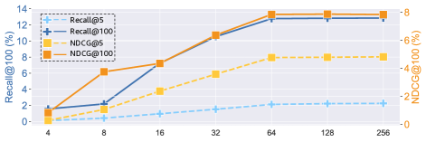
Figure 4. Experimental results of altering $S$ values.

3.2.2. Effect of Slicing Number $S$ (RQ2A).

Due to the renowned and stable performance of LightGCN (He et al., 2020), we utilize it as the backbone on AMZ-Book dataset to exemplify the model analysis. We alternatively change the value of $S$ and plot the results in Figure 4. We notice that, altering $S$ from $4$ to $64$ is more influential to the model performance, which is intuitive as this produces a more accurate and fine-grained cumulative approximation. However, on the other hand, consistently increasing $S$ will also put more computation and memory strains. Thus, setting $S$ as 64 is the balanced spot with positive momentum that presents a practical trade-off between model performance and resource consumption.

3.2.3. Dimension Reduction (RQ2B).

During evaluation, we notice that some models encounter the “out-of-memory” problem. To address this issue, we approach to aggregate layer-wise embeddings in Eqn.(7) to reduce the total dimensionality from $S(L+1)$ to $S$.

Table 3. Aggregation Selection.

Aggregator	Concat		Sum		Max
Metric	K=5	K=100	K=5	K=100	K=5	K=100
Recall@K	2.14	12.78	2.12	12.81	1.77	11.27
NDCG@K	4.77	7.85	4.78	7.77	4.31	7.01

From Table 3, we notice that Sum surprisingly presents a competitive performance with the original Concat operation. This indicates that, while Concat has a more complete representation encoding with theoretical supports, Sum is suitable for dimension reduction in scenarios with limited computational resources.

4. Conclusion and Future Extension

In this work, we propose WSFE to encode representations for effective user segmentation in collaborative filtering. The extensive experiments demonstrate the effectiveness of our proposed method and its generality to a variety of model deployments. As for future work, we point out three major directions as follows:

1. In light of the empirical findings in § 3.2.1, it is interesting to explore contrastive learning techniques (Zhang et al., 2023, 2022b; Ma et al., 2023; Liu et al., 2022b) in the sub-graph feature domain for further model improvement.

2. It is worth investigating adapting our training-free model to other scenarios of information retreival and autonomous database management (Qiu et al., 2022; Hu et al., 2020, 2021a; Liu et al., 2022a, 2023; Hu et al., 2021b; Shen et al., 2023c).

3. We plan to design unsupervised regularization mechanisms such that WSFE and the backbone model can be jointly optimized or even mutually enhanced for multi-task learning.

- (1)
- Amazon (2015) Amazon. 2015. Dataset. https://github.com/gusye1234/LightGCN-PyTorch/tree/master/data/amazon-book.
- Bonneel et al. (2015) Nicolas Bonneel, Julien Rabin, Gabriel Peyré, and Hanspeter Pfister. 2015. Sliced and radon wasserstein barycenters of measures. JMIV 51, 1 (2015), 22–45.
- Chen et al. (2023) Yankai Chen, Yixiang Fang, Yifei Zhang, and Irwin King. 2023. Bipartite Graph Convolutional Hashing for Effective and Efficient Top-N Search in Hamming Space. WebConf.
- Chen et al. (2022a) Yankai Chen, Huifeng Guo, Yingxue Zhang, Chen Ma, Ruiming Tang, Jingjie Li, and Irwin King. 2022a. Learning binarized graph representations with multi-faceted quantization reinforcement for top-k recommendation. In SIGKDD.
- Chen et al. (2022c) Yankai Chen, Menglin Yang, Yingxue Zhang, Mengchen Zhao, Ziqiao Meng, Jianye Hao, and Irwin King. 2022c. Modeling scale-free graphs with hyperbolic geometry for knowledge-aware recommendation. In WSDM. 94–102.
- Chen et al. (2022b) Yankai Chen, Yaming Yang, Yujing Wang, Jing Bai, Xiangchen Song, and Irwin King. 2022b. Attentive knowledge-aware graph convolutional networks with collaborative guidance for personalized recommendation. In ICDE.
- Cho et al. (2011) Eunjoon Cho, Seth A Myers, and Jure Leskovec. 2011. Friendship and mobility: user movement in location-based social networks. In SIGKDD. 1082–1090.
- Deshpande et al. (2019) Ishan Deshpande, Yuan-Ting Hu, Ruoyu Sun, Ayis Pyrros, Nasir Siddiqui, Sanmi Koyejo, Zhizhen Zhao, David Forsyth, and Alexander G Schwing. 2019. Max-sliced wasserstein distance and its use for gans. In CVPR. 10648–10656.
- Geng et al. (2015) Xue Geng, Hanwang Zhang, Jingwen Bian, and Tat-Seng Chua. 2015. Learning image and user features for recommendation in social networks. In ICCV. 4274–4282.
- Gowalla (2011) Gowalla. 2011. Dataset. https://github.com/gusye1234/LightGCN-PyTorch/tree/master/data/gowalla.
- Hamilton et al. (2017) William L Hamilton, Rex Ying, and Jure Leskovec. 2017. Inductive representation learning on large graphs. In NeurIPS. 1025–1035.
- He et al. (2023) Bowei He, Xu He, Yingxue Zhang, Ruiming Tang, and Chen Ma. 2023. Dynamically Expandable Graph Convolution for Streaming Recommendation. WebConf.
- He et al. (2020) Xiangnan He, Kuan Deng, Xiang Wang, Yan Li, Yongdong Zhang, and Meng Wang. 2020. Lightgcn: Simplifying and powering graph convolution network for recommendation. In SIGIR. 639–648.
- Hu et al. (2021a) Xuming Hu, Fukun Ma, Chenyao Liu, Chenwei Zhang, Lijie Wen, and Philip S Yu. 2021a. Semi-supervised Relation Extraction via Incremental Meta Self-Training. In EMNLP: Findings.
- Hu et al. (2020) Xuming Hu, Lijie Wen, Yusong Xu, Chenwei Zhang, and Philip S. Yu. 2020. SelfORE: Self-supervised Relational Feature Learning for Open Relation Extraction. In EMNLP. 3673–3682.
- Hu et al. (2021b) Xuming Hu, Chenwei Zhang, Yawen Yang, Xiaohe Li, Li Lin, Lijie Wen, and Philip S. Yu. 2021b. Gradient Imitation Reinforcement Learning for Low Resource Relation Extraction. In EMNLP. 2737–2746.
- Kindle (2015) Amazon Kindle. 2015. Dataset. https://github.com/Coder-Yu/SELFRec/tree/main/dataset/amazon-kindle.
- Kipf and Welling (2017) Thomas N Kipf and Max Welling. 2017. Semi-supervised classification with graph convolutional networks. ICLR.
- Kolouri et al. (2020) Soheil Kolouri, Navid Naderializadeh, Gustavo K Rohde, and Heiko Hoffmann. 2020. Wasserstein embedding for graph learning. ICLR.
- Kolouri et al. (2019) Soheil Kolouri, Kimia Nadjahi, Umut Simsekli, Roland Badeau, and Gustavo Rohde. 2019. Generalized sliced wasserstein distances. NeurIPS 32.
- Kolouri et al. (2016) Soheil Kolouri, Yang Zou, and Gustavo K Rohde. 2016. Sliced Wasserstein kernels for probability distributions. In CVPR. 5258–5267.
- Lee et al. (2021) Dongha Lee, SeongKu Kang, Hyunjun Ju, Chanyoung Park, and Hwanjo Yu. 2021. Bootstrapping user and item representations for one-class collaborative filtering. In SIGIR. 317–326.
- Li et al. (2019) Guohao Li, Matthias Muller, Ali Thabet, and Bernard Ghanem. 2019. Deepgcns: Can gcns go as deep as cnns?. In CVPR. 9267–9276.
- Lin et al. (2022) Zihan Lin, Changxin Tian, Yupeng Hou, and Wayne Xin Zhao. 2022. Improving graph collaborative filtering with neighborhood-enriched contrastive learning. In WebConf. 2320–2329.
- Ling et al. (2012) Guang Ling, Haiqin Yang, Irwin King, and Michael R Lyu. 2012. Online learning for collaborative filtering. In IJCNN. IEEE, 1–8.
- Liu et al. (2022a) Aiwei Liu, Xuming Hu, Li Lin, and Lijie Wen. 2022a. Semantic Enhanced Text-to-SQL Parsing via Iteratively Learning Schema Linking Graph. In SIGKDD. 1021–1030.
- Liu et al. (2023) Aiwei Liu, Xuming Hu, Lijie Wen, and Philip S Yu. 2023. A comprehensive evaluation of ChatGPT’s zero-shot Text-to-SQL capability. arXiv preprint arXiv:2303.13547 (2023).
- Liu et al. (2022b) Shuliang Liu, Xuming Hu, Chenwei Zhang, Shu’ang Li, Lijie Wen, and Philip S. Yu. 2022b. HiURE: Hierarchical Exemplar Contrastive Learning for Unsupervised Relation Extraction. In NAACL-HLT. 5970–5980.
- Luo et al. (2022) Fangyuan Luo, Jun Wu, and Tao Wang. 2022. Discrete Listwise Personalized Ranking for Fast Top-N Recommendation with Implicit Feedback. (2022).
- Ma et al. (2023) Yueen Ma, Zixing Song, Xuming Hu, Jingjing Li, Yifei Zhang, and Irwin King. 2023. Graph Component Contrastive Learning for Concept Relatedness Estimation. In AAAI.
- MovieLens (2003) MovieLens. 2003. Dataset. https://grouplens.org/datasets/movielens/1m/.
- Naderializadeh et al. (2021) Navid Naderializadeh, Joseph F Comer, Reed Andrews, Heiko Hoffmann, and Soheil Kolouri. 2021. Pooling by sliced-Wasserstein embedding. NeurIPS 34, 3389–3400.
- Pinterest (2015) Pinterest. 2015. Dataset. https://sites.google.com/site/xueatalphabeta/dataset-1/pinterest_iccv.
- Qiu et al. (2022) Zexuan Qiu, Qinliang Su, Jianxing Yu, and Shijing Si. 2022. Efficient Document Retrieval by End-to-End Refining and Quantizing BERT Embedding with Contrastive Product Quantization. EMNLP (2022).
- Rabin et al. (2011) Julien Rabin, Gabriel Peyré, Julie Delon, and Marc Bernot. 2011. Wasserstein barycenter and its application to texture mixing. In SSVM. Springer, 435–446.
- Shen et al. (2023a) Xin Shen, Kyungdon Joo, and Jean Oh. 2023a. FishRecGAN: An End to End GAN Based Network for Fisheye Rectification and Calibration. arXiv (2023).
- Shen et al. (2023b) Xin Shen, Jiaying Shi, Sungro Yoon, Jon Katzur, Hanbo Wang, Jim Chan, and Jin Li. 2023b. Learning to Personalize Recommendations based on Customers’ Shopping Intents. arXiv (2023).
- Shen et al. (2023c) Xin Shen, Xiaonan Zhao, and Rui Luo. 2023c. Semantic Embedded Deep Neural Network: A Generic Approach to Boost Multi-Label Image Classification Performance. arXiv (2023).
- Shen et al. (2023d) Xin Shen, Yan Zhao, Sujan Perera, Yujia Liu, Jinyun Yan, and Mitchell Goodman. 2023d. Learning Personalized Page Content Ranking Using Customer Representation. arXiv (2023).
- Song et al. (2021) Zixing Song, Ziqiao Meng, Yifei Zhang, and Irwin King. 2021. Semi-supervised Multi-label Learning for Graph-structured Data. In CIKM.
- Song et al. (2022) Zixing Song, Yifei Zhang, and Irwin King. 2022. Towards an Optimal Asymmetric Graph Structure for Robust Semi-supervised Node Classification. In SIGKDD. 1656–1665.
- Villani (2009) Cédric Villani. 2009. Optimal transport: old and new, Vol. 338. Springer.
- Wang et al. (2022) Chenyang Wang, Yuanqing Yu, Weizhi Ma, Min Zhang, Chong Chen, Yiqun Liu, and Shaoping Ma. 2022. Towards Representation Alignment and Uniformity in Collaborative Filtering. In SIGKDD. 1816–1825.
- Wang et al. (2019) Xiang Wang, Xiangnan He, Meng Wang, Fuli Feng, and Tat-Seng Chua. 2019. Neural graph collaborative filtering. In SIGIR. 165–174.
- Wu et al. (2020) Jun Wu, Fangyuan Luo, Yujia Zhang, and Haishuai Wang. 2020. Semi-discrete matrix factorization. IEEE Intelligent Systems 35, 5 (2020), 73–83.
- Wu et al. (2021) Jiancan Wu, Xiang Wang, Fuli Feng, Xiangnan He, Liang Chen, Jianxun Lian, and Xing Xie. 2021. Self-supervised graph learning for recommendation. In SIGIR. 726–735.
- Yang et al. (2022a) Menglin Yang, Zhihao Li, Min Zhou, Jiahong Liu, and Irwin King. 2022a. HICF: Hyperbolic informative collaborative filtering. In SIGKDD. 2212–2221.
- Yang et al. (2022b) Menglin Yang, Min Zhou, Jiahong Liu, Defu Lian, and Irwin King. 2022b. HRCF: Enhancing collaborative filtering via hyperbolic geometric regularization. In WebConf. 2462–2471.
- Yelp2018 (2018) Yelp2018. 2018. Dataset. https://github.com/gusye1234/LightGCN-PyTorch/tree/master/data/yelp2018.
- Ying et al. (2018) Rex Ying, Ruining He, Kaifeng Chen, Pong Eksombatchai, William L Hamilton, and Jure Leskovec. 2018. Graph convolutional neural networks for web-scale recommender systems. In SIGKDD. 974–983.
- Yu et al. (2022a) Junliang Yu, Hongzhi Yin, Xin Xia, Tong Chen, Lizhen Cui, and Quoc Viet Hung Nguyen. 2022a. Are graph augmentations necessary? simple graph contrastive learning for recommendation. In SIGIR. 1294–1303.
- Yu et al. (2022b) Junliang Yu, Hongzhi Yin, Xin Xia, Tong Chen, Jundong Li, and Zi Huang. 2022b. Self-Supervised Learning for Recommender Systems: A Survey. arXiv (2022).
- Zhang et al. (2022a) Xinni Zhang, Yankai Chen, Cuiyun Gao, Qing Liao, Shenglin Zhao, and Irwin King. 2022a. Knowledge-aware Neural Networks with Personalized Feature Referencing for Cold-start Recommendation. arXiv (2022).
- Zhang et al. (2023) Yifei Zhang, Yankai Chen, Zixing Song, and Irwin King. 2023. Contrastive Cross-scale Graph Knowledge Synergy. arXiv (2023).
- Zhang and Zhu (2020) Yifei Zhang and Hao Zhu. 2020. Discrete wasserstein autoencoders for document retrieval. In ICASSP. IEEE, 8159–8163.
- Zhang et al. (2022b) Yifei Zhang, Hao Zhu, Zixing Song, Piotr Koniusz, and Irwin King. 2022b. COSTA: Covariance-Preserving Feature Augmentation for Graph Contrastive Learning. In SIGKDD. 2524–2534.