A-ePA*SE: Anytime Edge-Based Parallel A* for Slow Evaluations

Abstract

Anytime search algorithms are useful for planning problems where a solution is desired under a limited time budget. Anytime algorithms first aim to provide a feasible solution quickly and then attempt to improve it until the time budget expires. On the other hand, parallel search algorithms utilize the multithreading capability of modern processors to speed up the search. One such algorithm, ePA*SE (Edge-Based Parallel A* for Slow Evaluations), parallelizes edge evaluations to achieve faster planning and is especially useful in domains with expensive-to-compute edges. In this work, we propose an extension that brings the anytime property to ePA*SE, resulting in A-ePA*SE. We evaluate A-ePA*SE experimentally and show that it is significantly more efficient than other anytime search methods. The open-source code for A-ePA*SE along with the baselines is available here: https://github.com/shohinm/parallel˙search

Introduction

Graph search algorithms are widely used in robotics for planning which can be formulated as the shortest path problem on a graph (Kusnur et al. 2021; Mukherjee et al. 2021). Parallelized graph search algorithms have shown to be effective in robotics domains where action evaluation tends to be expensive. In particular, a parallelized planning algorithm ePA*SE (Edge-based Parallel A* for Slow Evaluations) was developed (Mukherjee, Aine, and Likhachev 2022a) that changes the basic unit of the search from state expansions to edge expansions. This decouples the evaluation of edges from the expansion of their common parent state, giving the search the flexibility to figure out what edges need to be evaluated to solve the planning problem. Additionally, this provides a framework for the asynchronous parallelization of edge evaluations within the search.

Though parallelized planning algorithms achieve drastically lower planning times than their serial counterparts, for their applicability in real-time robotics, planning algorithms need to come up with a solution under a strict time budget. Though the optimal solution is preferable, that is often not the first priority. For such domains, anytime algorithms have been developed that first prioritize a quick feasible solution by allowing a high sub-optimality bound. This is typically done by incorporating a high inflation factor on the heuristic. They then attempt to improve the solution by incrementally decreasing the inflation factor and therefore tightening the sub-optimality bound until the time runs out. Therefore in this work, we bring the anytime property to ePA*SE. We show that the resulting algorithm, A-ePA*SE, achieves higher efficiency than existing anytime algorithms.

Related Work

Anytime algorithms

A naive approach to make wA* anytime is to sequentially run several iterations of it from scratch while reducing the heuristic inflation. Anytime A* (Zhou and Hansen 2002) finds an initial solution using wA* and then continues searching to improve the solution. A more elegant anytime algorithm Anytime Repairing A* (ARA*) (Likhachev, Gordon, and Thrun 2003a) reuses previous search efforts to prevent redundant work by keeping track of states whose cost-to-come can be further reduced in future iterations. Anytime Multi-heuristic A* (A-MHA*) (Natarajan et al. 2019) brings the anytime property to Multi-heuristic A* (Aine et al. 2016). Anytime Multi-resolution Multi-heuristic A* (AMRA*) (Saxena, Kusnur, and Likhachev 2022) is an anytime algorithm that searches over multiple resolutions of the state space. These algorithms, however, do not utilize any parallelization.

Parallel algorithms

Sampling-based methods like PRMs can be trivially parallelized (Amato and Dale 1999) by utilizing parallel processes cooperatively build the roadmap (Jacobs et al. 2012). Parallelized versions of RRT also exist in which multiple processes expand the search tree by sampling and adding multiple new states in parallel (Devaurs, Siméon, and Cortés 2011; Ichnowski and Alterovitz 2012; Jacobs et al. 2013; Park, Pan, and Manocha 2016). However, in many planning domains, sampling of states is not trivial, like in the case of domains that use a simulator in the loop (Liang et al. 2021). Parallelizing search-based methods are non-trivial because of their sequential nature. However, there have been several algorithms developed that achieve this. Parallel A* (Irani and Shih 1986) expands states in parallel while allowing re-expansions to maintain optimality, resulting in a high number of expansions. Several other approaches that parallelize state expansions suffer from this downside (Evett et al. 1995; Zhou and Zeng 2015; Burns et al. 2010), especially if they employ a weighted heuristic. In contrast, PA*SE (Phillips, Likhachev, and Koenig 2014) parallelly expands states at most once, in a way that does not affect the bounds on the solution quality. ePA*SE (Mukherjee, Aine, and Likhachev 2022a) improves PA*SE by changing the basic unit of the search from state expansions to edge expansions and then parallelizing this search over edges. GePA*SE (Mukherjee and Likhachev 2023) extends ePA*SE to domains where the actions are heterogenous in computational effort. A parallelized lazy planning algorithm, MPLP (Mukherjee, Aine, and Likhachev 2022b), achieves faster planning by running the search and evaluating edges asynchronously in parallel. There has also been work on parallelizing A* search on GPUs (Zhou and Zeng 2015; He et al. 2021) or multiple GPUs (He et al. 2021) by utilizing multiple parallel priority queues. These algorithms have a fundamental limitation that stems from the SIMD (single-instruction-multiple-data) execution model of a GPU, which limits their applicability to domains with simple actions that share the same code.

Problem Definition

Let a finite graph $G=(\mathcal{V},\mathcal{E})$ be defined as a set of vertices $\mathcal{V}$ and directed edges $\mathcal{E}$. Each vertex $v\in\mathcal{V}$ represents a state $\mathbf{s}$ in the state space of the domain $\mathcal{S}$. An edge $e\in\mathcal{E}$ connecting two vertices $v_{1}$ and $v_{2}$ in the graph represents an action $\mathbf{a}\in\mathcal{A}$ that takes the agent from corresponding states $\mathbf{s}_{1}$ to $\mathbf{s}_{2}$. In this work, we assume that all actions are deterministic. Hence an edge $e$ can be represented as a pair $(\mathbf{s},\mathbf{a})$, where $\mathbf{s}$ is the state at which action $\mathbf{a}$ is executed. For an edge $e$, we will refer to the corresponding state and action as $e.\mathbf{s}$ and $e.\mathbf{a}$ respectively. $\mathbf{s}_{0}$ is the start state and $\mathcal{G}$ is the goal region. $c:\mathcal{E}\rightarrow[0,\infty]$ is the cost associated with an edge. $g(\mathbf{s})$ or g-value is the cost of the best path to $\mathbf{s}$ from $\mathbf{s}_{0}$ found by the algorithm so far and $h(\mathbf{s})$ is a consistent heuristic (Russell 2010). Additionally, there exists a forward-backward consistent (Phillips, Likhachev, and Koenig 2014) pairwise heuristic function $h(\mathbf{s},\mathbf{s}^{\prime})$ that provides an estimate of the cost between any pair of states. A path $\pi$ is defined by an ordered sequence of edges $e_{i=1}^{N}=(\mathbf{s},\mathbf{a})_{i=1}^{N}$, the cost of which is denoted as $c(\pi)=\sum_{i=1}^{N}c(e_{i})$. The objective is to find a path $\pi$ from $\mathbf{s}_{0}$ to a state in the goal region $\mathcal{G}$ within a time budget $T$. There is a computational budget of $N_{t}$ threads available, which can run in parallel.

Method

We first describe ePA*SE and then the anytime extension to get to A-ePA*SE.

ePA*SE

Algorithm 1 A-ePA*SE: Plan

1:$\mathcal{A}\leftarrow\text{action space }$, $N_{t}\leftarrow$ thread budget, $T\leftarrow$ time budget

2:$w_{0}\leftarrow\text{initial heuristic weight}$, $\Delta w\leftarrow\text{delta heuristic weight }$

3:$G\leftarrow\text{graph}$, $\mathbf{s}_{0}\leftarrow\text{start state }$, $\mathcal{G}\leftarrow\text{goal region}$

4:$terminate\leftarrow\text{False}$

5:procedure Plan

6:     $\textit{INCON}\leftarrow\emptyset$

7:     $\forall\mathbf{s}\in G$, $\mathbf{s}.g\leftarrow\infty$

8:     $\mathbf{s}_{0}.g\leftarrow 0$, $w=w_{0}$

9:     insert $(\mathbf{s}_{0},\mathbf{a^{d}})$ in OPEN $\triangleright$ Dummy edge from $\mathbf{s}_{0}$

10:     while $w>=1$ and not $\textsc{Timeout}\left(T\right)$ do

11:         $\textit{INCON}=\emptyset,\textit{CLOSED}=\emptyset$

12:         $\textsc{ImprovePath}(w)$

13:         Publish current $w$ bounded sub-optimal solution

14:         $w=w-\Delta w$

15:         $\textit{OPEN}=\textit{OPEN}\cup\textit{INCON}$

16:         Re-balance OPEN with new $w$      

17:     $terminate=\text{True}$

Algorithm 2 A-ePA*SE: ImprovePath

1:procedure ImprovePath

2:     LOCK

3:     while $f(\mathbf{s}_{g})>min_{\mathbf{s}\in\textit{OPEN}}(f(\mathbf{s}))$ do

4:         if $\textit{OPEN}=\emptyset\textbf{ and }\textit{BE}=\emptyset$ then

5:              UNLOCK

6:              $\textbf{return}{}~{}\emptyset$          

7:         remove an edge $(\mathbf{s},\mathbf{a})$ from OPEN that has the
          smallest $f((\mathbf{s},\mathbf{a}))$ among all states in OPEN that
          satisfy Equations 1 and 2

8:         if such an edge does not exist then

9:              UNLOCK

10:              wait until OPEN or BE change

11:              LOCK

12:              continue          

13:         if $\mathbf{s}\in\mathcal{G}$ and $f(\mathbf{s}_{g})>f(\mathbf{s})$ then

14:              $\mathbf{s}_{g}=\mathbf{s}$

15:              $plan=\textsc{Backtrack($\mathbf{s}$)}$          

16:         UNLOCK

17:         while $(\mathbf{s},\mathbf{a})$ has not been assigned a thread do

18:              for $i=1:N_{t}$ do

19:                  if thread $i$ is available then

20:                       if thread $i$ has not been spawned then

21:                           Spawn $\textsc{EdgeExpandThread}(i)$                        

22:                       Assign $(\mathbf{s},\mathbf{a})$ to thread $i$                                          

23:         LOCK      

24:     UNLOCK

25:     $\textbf{return}{}~{}plan$

Algorithm 3 A-ePA*SE: Edge Expansion

1:procedure EdgeExpandThread($i$)

2:     while $\textbf{not }terminate$ do

3:         if thread $i$ has been assigned an edge $(\mathbf{s},\mathbf{a})$ then

4:              $\textsc{Expand}\left((\mathbf{s},\mathbf{a})\right)$               

5:procedure Expand($(\mathbf{s},\mathbf{a})$)

6:     LOCK

7:     if $\mathbf{a}=\mathbf{a^{d}}$ then

8:         insert $\mathbf{s}$ in BE

9:         for $\mathbf{a}\in\mathcal{A}$ do

10:              $f\left((\mathbf{s},\mathbf{a})\right)=g(\mathbf{s})+h(\mathbf{s})$

11:              insert $(\mathbf{s},\mathbf{a})$ in OPEN with $f\left((\mathbf{s},\mathbf{a})\right)$          

12:     else

13:         UNLOCK

14:         if  $\textsc{NotEvaluated}\left((\mathbf{s},\mathbf{a})\right)$  then

15:              $\mathbf{s}^{\prime},c\left((\mathbf{s},\mathbf{a})\right)\leftarrow\textsc{GenerateSuccessor}\left((\mathbf{s},\mathbf{a})\right)$

16:         else

17:              $\mathbf{s}^{\prime},c\left((\mathbf{s},\mathbf{a})\right)\leftarrow\textsc{GetSuccessor}\left((\mathbf{s},\mathbf{a})\right)$          

18:         LOCK

19:         if $g(\mathbf{s}^{\prime})>g(\mathbf{s})+c\left((\mathbf{s},\mathbf{a})\right)$ then

20:              $g(\mathbf{s}^{\prime})=g(\mathbf{s})+c\left((\mathbf{s},\mathbf{a})\right)$

21:              $f\left((\mathbf{s}^{\prime},\mathbf{a^{d}})\right)=g(\mathbf{s}^{\prime})+wh(\mathbf{s}^{\prime})$

22:              if $\mathbf{s}^{\prime}\notin\textit{CLOSED}\cup\textit{BE}$ then

23:                  update $(\mathbf{s}^{\prime},\mathbf{a^{d}})$ in OPEN with $f\left((\mathbf{s}^{\prime},\mathbf{a^{d}})\right)$

24:              else

25:                  update $(\mathbf{s}^{\prime},\mathbf{a^{d}})$ in INCON with $f\left((\mathbf{s}^{\prime},\mathbf{a^{d}})\right)$                        

26:         $n\_successors\_generated(\mathbf{s})+=1$

27:         if $n\_successors\_generated(\mathbf{s})=|\mathcal{A}|$ then

28:              remove $\mathbf{s}$ from BE

29:              insert $\mathbf{s}$ in CLOSED               

30:     UNLOCK

In A*, during a state expansion, all its successors are generated and are inserted/repositioned in the open list. In ePA*SE, the open list (OPEN) is a priority queue of edges (not states) that the search has generated but not expanded, where the edge with the smallest key/priority is placed in the front of the queue. The priority of an edge $e=(\mathbf{s},\mathbf{a})$ in OPEN is $f\left((\mathbf{s},\mathbf{a})\right)=g(\mathbf{s})+h(\mathbf{s})$. Expansion of an edge $(\mathbf{s},\mathbf{a})$ involves evaluating the edge to generate the successor $\mathbf{s}^{\prime}$ and adding/updating (but not evaluating) the edges originating from $\mathbf{s}^{\prime}$ into OPEN with the same priority of $g(\mathbf{s}^{\prime})+h(\mathbf{s}^{\prime})$. Henceforth, whenever $g(\mathbf{s}^{\prime})$ changes, the positions of all of the outgoing edges from $\mathbf{s}^{\prime}$ need to be updated in OPEN. To avoid this, ePA*SE replaces all the outgoing edges from $\mathbf{s}^{\prime}$ by a single dummy edge $(\mathbf{s}^{\prime},\mathbf{a^{d}})$, where $\mathbf{a^{d}}$ stands for a dummy action until the dummy edge is expanded. Every time $g(\mathbf{s}^{\prime})$ changes, only the dummy edge has to be repositioned. Unlike what happens when a real edge is expanded, when the dummy edge $(\mathbf{s}^{\prime},\mathbf{a^{d}})$ is expanded, it is replaced by the outgoing real edges from $\mathbf{s}^{\prime}$ in OPEN. This is also when the state $\mathbf{s}^{\prime}$ is considered to be under expansion. The real edges are expanded when they are popped from OPEN by an edge expansion thread. This means that every edge gets delegated to a separate thread for expansion. $\mathbf{s}^{\prime}$ is marked expanded (Line 29, Alg.  3) when all outgoing edges are expanded.

A single thread runs the main planning loop (Alg. 2) and pulls out edges from OPEN, and delegates their expansion to an edge expansion thread (Alg.3). To maintain optimality, an edge can only be expanded if it is independent of all edges ahead of it in OPEN and the edges currently being expanded, i.e., in set BE (Mukherjee, Aine, and Likhachev 2022a). An edge $e$ is independent of another edge $e^{\prime}$ if the expansion of $e^{\prime}$ cannot possibly reduce $g(e.\mathbf{s})$. Formally, this independence check is expressed by Inequalities 1 and 2. w-ePA*SE is a bounded suboptimal variant of ePA*SE that trades off optimality for faster planning by introducing two inflation factors. $w\geq 1$ inflates the priority of edges in OPEN i.e. $f\left((\mathbf{s},\mathbf{a})\right)=g(\mathbf{s})~{}+~{}wh(\mathbf{s})$. $\epsilon\geq 1$ used in Inequalities 1 and  2 relaxes the independence rule. As long as $\epsilon\geq w$, the solution cost is bounded by $\epsilon\cdot c^{*}$. We let $\epsilon=w$ in this work, so we have one variable to control the suboptimality bound.

$$\begin{split}g(e.\mathbf{s})-g(e^{\prime}.\mathbf{s})\leq\epsilon h(e^{\prime}.\mathbf{s},e.\mathbf{s})\\ \forall e^{\prime}\in\textit{OPEN}~{}|~{}f\left(e^{\prime}\right)<f\left(e\right)\end{split}$$ (1)

$$\begin{split}g(e.\mathbf{s})-g(\mathbf{s}^{\prime})\leq\epsilon h(\mathbf{s}^{\prime},e.\mathbf{s})~{}\forall\mathbf{s}^{\prime}\in\textit{BE}\end{split}$$ (2)

A-ePA*SE

Inspired by ARA*, we extend w-ePA*SE to a parallelized anytime repairing algorithm A-ePA*SE by inheriting three algorithmic techniques:

1. Define locally inconsistent states as the states whose $g$-values change while they are in $\textit{CLOSED}\cup\textit{BE}$ during the current ImprovePath execution ((Likhachev, Gordon, and Thrun 2003a)). A-ePA*SE keeps track of locally inconsistent states by maintaining an inconsistent list INCON (Line 25, Alg. 3).

2. After every $i^{th}$ ImprovePath call exits, A-ePA*SE initializes OPEN for the next search iteration $i+1$ as $\textit{OPEN}_{i+1}=\textit{OPEN}_{i}\cup\textit{INCON}$ . (Line 15, Alg.1).

3. A-ePA*SE changes the termination condition of a search iteration (Line 3, Alg.2) so that it only expands states that 1) have $g$-value that can be lowered in the current ImprovePath iteration or 2) were locally inconsistent in the previous ImprovePath iteration.

A-ePA*SE extends w-ePA*SE with an additional outer control loop (Alg. 1) that sequentially reduces $w$. In the first iteration, ImprovePath is called with $w_{0}$. This is equivalent to running w-ePA*SE except for the algorithmic change described in technique 1. When ImprovePath returns, the current $w$-suboptimal solution is published (Line 13, Alg. 1). Before every subsequent call to ImprovePath, $w$ is reduced by $\Delta w$ and OPEN is updated as described in technique 2. It is possible that no or very few states in OPEN satisfy the termination check stated in technique 3 and ImprovePath returns right away or after a few expansions. This reusing of previous search effort is the fundamental source of efficiency gains for A-ePA*SE as compared to running w-ePA*SE from scratch with a reduced $w$. A-ePA*SE terminates when either 1) the time budget expires, and the current best solution is returned or 2) ImprovePath finds a provably optimal solution with $w=1$.

Properties

Theorem 1

(Anytime correctness) Each time the ImprovePath function exits, the following holds: the cost of a greedy path from $\mathbf{s}_{0}$ to $\mathbf{s}_{g}$ is no larger than $\lambda g^{*}(\mathbf{s}_{g})$, where $\lambda=\max(\epsilon,w)$.

Theorem 2

(Anytime efficiency) Within each call to ImprovePath a state $\mathbf{s}$ is expanded only if it was already locally inconsistent before the call to ImprovePath or its $g$-value was lowered during the current execution of ImprovePath.

Proof sketch These properties were proved for each ImprovePath function call in ARA* (Corollary 13 & Theorem 2 in (Likhachev, Gordon, and Thrun 2003b)) with $\lambda=w$. The anytime correctness properties are also proved for a single w-ePA*SE run (Theorem 3 in (Mukherjee, Aine, and Likhachev 2022a)) with $\lambda=\max(\epsilon,w)$. Since we are inheriting the method to repair the graph and reuse the search effort of ARA*, these properties similarly follow for each ImprovePath function call in A-ePA*SE.

Evaluation

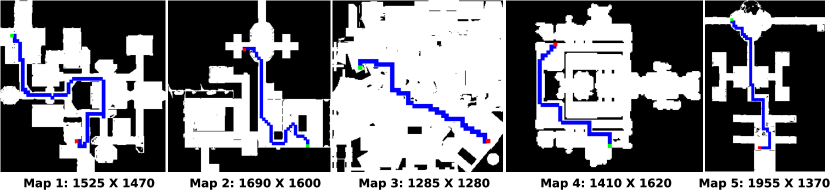
Figure 1: MovingAI maps with the start state shown in green, the goal state shown in red, and the computed path shown in blue.

We use 5 scaled MovingAI 2D maps (Sturtevant 2012), with state space being 2D grid coordinates shown in Fig. 1. The agent has a square footprint with a side length of 32 units. The action space comprises moving along 8 directions by 25 cell units. To check action feasibility, we collision-check the footprint at interpolated states with a 1-unit discretization. For each map, we sample 50 random start-goal pairs and verify that there exists a solution by running wA* with a large timeout. All algorithms use Euclidean distance as the heuristic. We run the experiments with two cost maps: 1) Euclidean cost and 2) Euclidean cost multiplied with a random factor map generated by sampling a uniform distribution between 1 and 100. In the random cost map, there is a tendency for the solution to be improved more gradually with the decrease in $w$. In the case of Euclidean cost, the solution tends to improve only from one topology to another with a $w$ decrease, yielding fewer intermediate suboptimal solutions. We compare A-ePA*SE with three baselines: 1) ARA* 2) ePA*SE and 3) A-ePA*SE-naive, which runs w-ePA*SE sequentially with decreasing $w$ without reuse of previous search effort. For the anytime algorithms, $w_{0}$ is set to 50, and $\Delta w$ is set to 0.5. All experiments were carried out on an AMD Threadripper Pro 5995WX workstation with a thread budget of 120. In all cases, we keep a high time budget, so none of the algorithms timeout.

	Euclidean Cost			Random Cost
	$\hat{t}_{init}$	$\hat{t}_{opt}$	$\hat{t}_{term}$	$\hat{t}_{init}$	$\hat{t}_{opt}$	$\hat{t}_{term}$
ARA*	19 (0.923)	47	50	41 (0.902)	99	178
ePA*SE	11	11	11	38	38	38
A-ePA*SE-naive	6 (0.948)	159	200	10 (0.951)	396	767
A-ePA*SE	6 (0.949)	14	16	10 (0.954)	27	44
	$\hat{s}_{init}$	$\hat{s}_{opt}$	$\hat{s}_{term}$	$\hat{s}_{init}$	$\hat{s}_{opt}$	$\hat{s}_{term}$
ARA*	2.69	3.62	2.89	3.52	3.70	3.88
ePA*SE	1.75	1.00	0.70	4.17	1.82	0.86
A-ePA*SE-naive	0.98	9.19	11.94	1.01	13.12	16.44

Table 1: Top: Mean time ($\mathrm{ms}$) to find the initial feasible solution ($\hat{t}_{init}$), discover optimal solution ($\hat{t}_{opt}$) and prove optimal solution ($\hat{t}_{term}$). Numbers in parenthesis in the $\hat{t}_{init}$ columns are the initial optimality ratios. Bottom: Speedup of A-ePA*SE over the baselines.

Table 1 top shows raw planning times for three stages. $\hat{t}_{init}$ is the mean time to generate the first solution, $\hat{t}_{opt}$ is the mean time to first discover the optimal solution in hindsight, and $\hat{t}_{term}$ is the mean time to provably generate the optimal solution by the final ImprovePath call with $w=1$. Table 1 bottom presents the average speedup of A-ePA*SE over the baselines (${t}_{baseline}/{t}_{A-ePA*SE}$). This is generated by computing the speedup for each run and then averaging them over all runs and all maps. A-ePA*SE-naive and A-ePA*SE compute the initial solution faster than ARA* due to parallelization and than ePA*SE due to the high inflation on the heuristic. A-ePA*SE computes the provably optimal solution quicker than A-ePA*SE-naive and ARA*, but slower than ePA*SE. This is expected since ePA*SE is not an anytime algorithm and runs a single optimal search. However, A-ePA*SE can discover the optimal solution in hindsight faster than ePA*SE in the random cost map. This means that even if the time budget runs out before the A-ePA*SE runs its final iteration with $w=1$ to provably generate the optimal plan and the robot executes the best plan so far, it may still end up behaving optimally. This is an important and useful empirical result for real-time robotics.

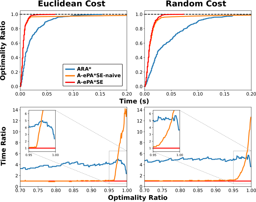
Figure 2: Top: The mean optimality ratio an algorithm achieves at a specific time point. Bottom: Planning times of the baselines divided by that of A-ePA*SE to achieve the same mean optimality ratio. In other words, for a specific algorithm, the bottom plots show how much slower (y-axis) than A-ePA*SE that algorithm gets to a solution that has a specific optimality factor (x-axis). The plot in the 0.95-1.00 optimality range is zoomed into.

Fig. 2 (top) shows the optimality ratio (optimal cost / actual cost) achieved by an anytime algorithm at a specific time point. For every problem, we calculate the optimality ratio at every time point when ImprovePath returns. We then discretize time and assign each time point with the best optimality ratio achieved so far. This is then averaged across all maps and problems separately for the two different cost maps. To show the relative performance, Fig. 2 (bottom) divides the time it takes the baselines to achieve a given optimality ratio by the time of A-ePA*SE to achieve the same optimality ratio. Specifically, the plot represents how many times slower an algorithm is than A-ePA*SE in computing a solution with a certain optimality factor represented by the x-axis. We see that ARA* takes significantly longer to reach the same optimality ratio as compared to A-ePA*SE. A-ePA*SE-naive does as good as A-ePA*SE for lower optimality ratios, but it takes significantly longer to achieve optimality because it does not reuse previous search effort. A-ePA*SE outperforms ARA* as predicted due to the efficiency gained from parallelization.

Summary of results

The experimental evaluation demonstrates the advantages of A-ePA*SE over the baselines.

• Compared to ARA*, both Fig. 2 and Table. 1 indicate that A-ePA*SE outperforms ARA* in planning time.

• As shown in Table 1, A-ePA*SE and A-ePA*SE-naive both find the initial solution at around 0.95 optimality. This implies that, on average, the solution cost improvement primarily happens in the 0.95-1.0 optimality range, making it the range of interest for analysis. Fig. 2 (zoomed in) shows that A-ePA*SE improves the optimality ratio quicker than A-ePA*SE-naive in the that range region.

• Compared to ePA*SE, A-ePA*SE has an anytime behavior where it quickly computes a feasible solution and then improves it over time. Additionally, it computes the optimal solution in hindsight ($\hat{t}_{opt}$) faster than ePA*SE in the random cost map, which is a useful insight in the real-time robotics context.

Conclusion and Future Work

In this work, we present an anytime parallelized search algorithm A-ePA*SE. Our experiments demonstrated that A-ePA*SE achieves a significant speedup over ARA* in both computing an initial solution and then improving it to compute the optimal solution. Additionally, the anytime property of A-ePA*SE makes it potentially more useful than ePA*SE in a range of real-time robotics domains. In the current formulation of A-ePA*SE, both the initial heuristic inflation $w_{0}$ and the decrement $\Delta w$ between successive ImprovePath calls are parameters to be tuned. In the future, A-ePA*SE can be extended to a non-parametric formulation.

References

- Aine et al. (2016) Aine, S.; Swaminathan, S.; Narayanan, V.; Hwang, V.; and Likhachev, M. 2016. Multi-heuristic A*. The International Journal of Robotics Research, 35(1-3): 224–243.
- Amato and Dale (1999) Amato, N. M.; and Dale, L. K. 1999. Probabilistic roadmap methods are embarrassingly parallel. In Proceedings 1999 IEEE International Conference on Robotics and Automation, volume 1, 688–694.
- Burns et al. (2010) Burns, E.; Lemons, S.; Ruml, W.; and Zhou, R. 2010. Best-first heuristic search for multicore machines. Journal of Artificial Intelligence Research, 39: 689–743.
- Devaurs, Siméon, and Cortés (2011) Devaurs, D.; Siméon, T.; and Cortés, J. 2011. Parallelizing RRT on distributed-memory architectures. In 2011 IEEE International Conference on Robotics and Automation, 2261–2266.
- Evett et al. (1995) Evett, M.; Hendler, J.; Mahanti, A.; and Nau, D. 1995. PRA*: Massively parallel heuristic search. Journal of Parallel and Distributed Computing, 25(2): 133–143.
- He et al. (2021) He, X.; Yao, Y.; Chen, Z.; Sun, J.; and Chen, H. 2021. Efficient parallel A* search on multi-GPU system. Future Generation Computer Systems, 123: 35–47.
- Ichnowski and Alterovitz (2012) Ichnowski, J.; and Alterovitz, R. 2012. Parallel sampling-based motion planning with superlinear speedup. In IROS, 1206–1212.
- Irani and Shih (1986) Irani, K.; and Shih, Y.-f. 1986. Parallel A* and AO* algorithms- An optimality criterion and performance evaluation. In 1986 International Conference on Parallel Processing, University Park, PA, 274–277.
- Jacobs et al. (2012) Jacobs, S. A.; Manavi, K.; Burgos, J.; Denny, J.; Thomas, S.; and Amato, N. M. 2012. A scalable method for parallelizing sampling-based motion planning algorithms. In 2012 IEEE International Conference on Robotics and Automation, 2529–2536.
- Jacobs et al. (2013) Jacobs, S. A.; Stradford, N.; Rodriguez, C.; Thomas, S.; and Amato, N. M. 2013. A scalable distributed RRT for motion planning. In 2013 IEEE International Conference on Robotics and Automation, 5088–5095.
- Kusnur et al. (2021) Kusnur, T.; Mukherjee, S.; Saxena, D. M.; Fukami, T.; Koyama, T.; Salzman, O.; and Likhachev, M. 2021. A planning framework for persistent, multi-uav coverage with global deconfliction. In Field and Service Robotics, 459–474. Springer.
- Liang et al. (2021) Liang, J.; Sharma, M.; LaGrassa, A.; Vats, S.; Saxena, S.; and Kroemer, O. 2021. Search-Based Task Planning with Learned Skill Effect Models for Lifelong Robotic Manipulation. arXiv preprint arXiv:2109.08771.
- Likhachev, Gordon, and Thrun (2003a) Likhachev, M.; Gordon, G. J.; and Thrun, S. 2003a. ARA*: Anytime A* with provable bounds on sub-optimality. Advances in neural information processing systems, 16.
- Likhachev, Gordon, and Thrun (2003b) Likhachev, M.; Gordon, G. J.; and Thrun, S. 2003b. Ara: formal analysis.
- Mukherjee, Aine, and Likhachev (2022a) Mukherjee, S.; Aine, S.; and Likhachev, M. 2022a. ePA*SE: Edge-Based Parallel A* for Slow Evaluations. In International Symposium on Combinatorial Search, volume 15, 136–144. AAAI Press.
- Mukherjee, Aine, and Likhachev (2022b) Mukherjee, S.; Aine, S.; and Likhachev, M. 2022b. MPLP: Massively Parallelized Lazy Planning. IEEE Robotics and Automation Letters, 7(3): 6067–6074.
- Mukherjee and Likhachev (2023) Mukherjee, S.; and Likhachev, M. 2023. GePA* SE: Generalized Edge-Based Parallel A* for Slow Evaluations. arXiv preprint arXiv:2301.10347.
- Mukherjee et al. (2021) Mukherjee, S.; Paxton, C.; Mousavian, A.; Fishman, A.; Likhachev, M.; and Fox, D. 2021. Reactive long horizon task execution via visual skill and precondition models. In 2021 IEEE/RSJ International Conference on Intelligent Robots and Systems (IROS), 5717–5724. IEEE.
- Natarajan et al. (2019) Natarajan, R.; Saleem, M.; Aine, S.; Likhachev, M.; and Choset, H. 2019. A-MHA*: anytime multi-heuristic A. In Proceedings of the International Symposium on Combinatorial Search, volume 10, 192–193.
- Park, Pan, and Manocha (2016) Park, C.; Pan, J.; and Manocha, D. 2016. Parallel motion planning using poisson-disk sampling. IEEE Transactions on Robotics, 33(2): 359–371.
- Phillips, Likhachev, and Koenig (2014) Phillips, M.; Likhachev, M.; and Koenig, S. 2014. PA* SE: Parallel A* for slow expansions. In Twenty-Fourth International Conference on Automated Planning and Scheduling.
- Russell (2010) Russell, S. J. 2010. Artificial intelligence a modern approach. Pearson Education, Inc.
- Saxena, Kusnur, and Likhachev (2022) Saxena, D. M.; Kusnur, T.; and Likhachev, M. 2022. AMRA*: Anytime Multi-Resolution Multi-Heuristic A. In 2022 International Conference on Robotics and Automation (ICRA), 3371–3377. IEEE.
- Sturtevant (2012) Sturtevant, N. 2012. Benchmarks for Grid-Based Pathfinding. Transactions on Computational Intelligence and AI in Games, 4(2): 144 – 148.
- Zhou and Hansen (2002) Zhou, R.; and Hansen, E. A. 2002. Multiple Sequence Alignment Using Anytime A*. In AAAI/IAAI, 975–977.
- Zhou and Zeng (2015) Zhou, Y.; and Zeng, J. 2015. Massively parallel A* search on a GPU. In Proceedings of the AAAI Conference on Artificial Intelligence.