Traversable Morris-Thorne-Buchdahl wormholes in quadratic gravity

Abstract

The special Buchdahl-inspired metric obtained in a recent paper [Phys. Rev. D 107, 104008 (2023)] describes asymptotically flat spacetimes in pure $\mathcal{R}^{2}$ gravity. The metric depends on a new (Buchdahl) parameter $\tilde{k}$ of higher-derivative characteristic, and recovers the Schwarzschild metric when $\tilde{k}=0$. It is shown that the special Buchdahl-inspired metric supports a two-way traversable Morris-Thorne wormhole for $\tilde{k}\in(-1,0)$ in which case the Weak Energy Condition is formally violated, a naked singularity for $\tilde{k}\in(-\infty,-1)\cup(0,+\infty)$, and a non-Schwarzschild structure for $\tilde{k}=-1$.

I Introduction

Recently, there has been a surge in interest in wormholes, particularly with the Morris-Thorne ansatz as a guiding principle (MorrisThorne-1988-1, ; MorrisThorne-1988-2, ). Supermassive objects have been discovered and used as a test bed for gravity, and although wormholes are of an exotic nature, they may interact with ordinary matter and can be observed via their astrophysical signatures (Darmour, ; Bambi, ; Azreg, ; Dzhunushaliev, ; Cardoso, ; Konoplya, ; Nandi, ; Bueno, ; Cramer, ; Nedkova, ; Harko, ; Deligianni, ; Falco, ; p4, ; p5, ; Easson-2015, ; Easson-2017, ). As a result, it is natural to seek, static and rotating (p1, ; p2, ; p3, ; p6, ; p7, ), wormholes in modified theories of gravity that permit a violation of the Weak Energy Condition (WEC) without assuming the existence of exotic matter.

All we know about exotic matter is that a) it violates our perception of energy, that is, an observer may measure some negative amount of rest energy density and b) it has the ability to sustain wormholes. So far there has been no general theory about exotic matter and most of–if not all–the wormhole solutions derived so far were obtained geometrically upon running the field equations of general relativity (GR) from left to right: The energy-momentum tensor (EMT) derived this way was exotic. In this work we rather run the field equations of purely quadratic gravity in the usual way, that is, by solving the field equations.

In generalized and modified theories of GR, explicit EMT are not usually added to the field equations. Instead, extra terms or corrections are introduced to the gravitation sector, which can play the role of exotic matter without truly being exotic matter. An example is the Brans-Dicke (BD) action, $\int d^{4}x\sqrt{-g}\left[\phi\,\mathcal{R}-\frac{\omega}{\phi}\partial_{\mu}\phi\partial^{\mu}\phi\right]$, which allows the formation of wormholes (Agnese-1995, ; Agnese-2001, ; Campanelli-1993, ; Vanzo-2012, ), where the scalar field $\phi$ acts as an exotic form of matter that violates the WEC. Another interesting case is the family of $f(\mathcal{R})$ gravity, which in general can be formally cast as a scalar-tensor theory but the scalar field is directly associated with $\mathcal{R}$ without its own dynamics. As such, the scalar field does not truly represent an exotic form of matter. In the case of pure $\mathcal{R}^{2}$ gravity, the scalar field is trivially identical to $\mathcal{R}$.

Violation of the energy conditions, and particularly of the WEC, has direct astrophysical consequences. In  (wec1, ) it was shown how the non-violation of the WEC constrains the time evolution of both the Hubble parameter and coordinate distance and sets an upper bound for $\Omega_{M}$. Similar conclusions were derived in  (wec2, ). In the other case, when the WEC is violated, no such constraints emerge. Assuming that the SEC and the DEC hold, a first proof of the Cosmic No-Hair Theorem was given in  (wec3, ). Another theorem on the future fate of a spacetime, the Lorentzian Splitting Theorem, was proven upon admitting the SEC  (wec4, ). From a quantum-mechanical point of view, all local energy conditions are violated by quantum fields and also by some classical fields as the non-minimally coupled scalar fields  (wec5, ; wec6, ) and the future-eternal inflating spacetimes  (wec7, ). However, the scale of violation can be minimized for some cut-and-paste geometric constructions  (wec8, ), and for type I wormholes without the cut-and-paste construction  (Azreg, ) where the extent of exotic matter has been shown to be inversely proportional to the square of the mass of the wormhole. A detailed compte-rendu of the consequences and plausible violations of the energy conditions are reported in  (wec9, ), instances include the possibility of formation of cosmological singularities in spatially open or flat spacetimes if the WEC is observed and the possibility of superluminal motion (wrap drive and traversable wormholes) if the WEC is violated.

The pure $\mathcal{R}^{2}$ theory was first proposed by Buchdahl in the early 1960’s (Buchdahl-1962, ) and has recently experienced a revival of interest, with active investigations into its theoretical properties as well as its implications for black holes and cosmology (Lust-2015-backholes, ; Clifton-2006, ; Ferreira-2019, ; Stelle-2015, ; Pravda-2017, ; Nguyen-2022-Buchdahl, ; 2023-axisym, ; 2023-WH, ; Alvarez-2018, ; Rinaldi-2018, ; Donoghue-2018, ; Gurses-2012, ; Frolov-2009, ; Stelle-1977, ; Nguyen-2023-Lambda0, ; Nguyen-2023-Extension, ; Nguyen-2023-Nontrivial, ; Murk-2022, ; Nelson-2010, ). Among the various extensions of GR, the pure $\mathcal{R}^{2}$ theory enjoys several distinct advantages. It is a parsimonious theory, having only one term in the action, $(2\kappa)^{-1}\int d^{4}x\sqrt{-g}\,\mathcal{R}^{2}$, where the gravitational coupling $\kappa$ is a dimensionless parameter. It is the only theory that is both scale invariant and ghost-free. Regarding the former, it actually possesses a restricted scale invariance under a Weyl transformation, $g_{\mu\nu}\rightarrow\Omega^{2}(x)g_{\mu\nu}$, where $\Omega(x)$ obeys a harmonic condition, $\square\,\Omega=0$, as discovered in (Edery-2014, ). Regarding the latter, as a member of $f(\mathcal{R})$, its scalar degree of freedom involves only second-order derivatives when transitioning from the Jordan frame to the Einstein frame, thereby evading the Ostrogradsky instability that often plagues higher-derivative gravity (Woodard, ). Furthermore, pure $\mathcal{R}^{2}$ gravity has been shown propagate two massless modes: a spin-2 tensor mode and a spin-0 scalar mode, each carrying it own significance (AlvarezGaume-2015, ). On one hand, the massless spin-2 tensor mode indicates the emergence of a long-range potential with the correct Newtonian tail $\sim 1/r$ (Nguyen-2023-Newtonian, ). On the other hand, the massless spin-0 scalar mode could potentially be responsible for an additional long-range potential, thereby introducing new physics.

One concrete realization of new physics in pure $\mathcal{R}^{2}$ gravity manifests through the work of Buchdahl in 1962, in which he originated a program aimed at finding vacuum solutions for the theory (Buchdahl-1962, ). He was able to make significant progress with his efforts boiling down to solving a non-linear second-order ordinary differential equation (ODE). If an analytical solution to his ODE could be found, then the vacuo solutions he sought would automatically ensue. Unfortunately, Buchdahl deemed the ODE insoluble, prompting him to suspend further pursuit. Consequently, his groundbreaking paper has remained relatively obscure within the gravitational research community for the past sixty years. However, recent advancements made by one of us have revitalized Buchdahl’s program and brought it to fruition. Section II in this paper will review its final outcome.

Significantly, the Buchdahl-inspired solutions exhibit non-constant scalar curvature, a distinctive feature resulting from the fourth-derivative nature of the theory. This non-constant scalar curvature is controlled by a new parameter known as the Buchdahl parameter $k$. Remarkably, these solutions defy the generalized Lichnerowicz “theorem” proposed in (Nelson-2010, ; Stelle-2015, ; Lust-2015-backholes, ), which stipulates that static vacuum solutions of pure $\mathcal{R}^{2}$ gravity must possess constant scalar curvature exclusively. The Buchdahl-inspired solutions evade this “theorem” by circumventing one of the central assumptions (Nguyen-2023-Extension, ). The non-constant scalar curvature observed in these solutions is a manifestation of higher-derivative effects, which are encapsulated by the Buchdahl parameter $k$.

In this paper, we shall use the closed analytical vacuum solution for pure $\mathcal{R}^{2}$ gravity derived in Ref.  (Nguyen-2023-Lambda0, ) to show the formation of a wormhole that connects two asymptotically flat spacetime sheets via a “throat”. This wormhole is enabled by the high-derivative nature of the theory without requiring complicated ingredients or true exotic matter.

The paper is structured as follows. In Sec. II we review Buchdahl-inspired metrics obtained in Refs.  (Nguyen-2022-Buchdahl, ; Nguyen-2023-Lambda0, ; Nguyen-2023-Nontrivial, ); in Sec. III we present two additional representations for Buchdahl-inspired metrics that are asymptotically flat; in Sec. IV we map the special (asymptotically flat) Buchdahl-inspired metrics to the Morris-Thorne ansatz, investigate their properties, and construct a wormhole when the Weak Energy Condition is violated.

II Buchdahl-inspired $\mathcal{R}^{2}$ spacetimes

In Ref.  (Nguyen-2022-Buchdahl, ) we advanced a program initiated by Buchdahl in 1962 seeking vacuo configurations for pure $\mathcal{R}^{2}$ gravity (Buchdahl-1962, ). The field equation in vacuo

$$\mathcal{R}\left(\mathcal{R}_{\mu\nu}-\frac{1}{4}g_{\mu\nu}\mathcal{R}\right)+\left(g_{\mu\nu}\square-\nabla_{\mu}\nabla_{\nu}\right)\mathcal{R}=0$$ (1)

has a static spherisymmetric solution which is expressible in terms of two auxiliary functions $p(r)$ and $q(r)$ per

$$ds^{2}=e^{k\int\frac{dr}{r\,q(r)}}\left\{-\frac{p(r)q(r)}{r}dt^{2}+\frac{p(r)\,r}{q(r)}dr^{2}+r^{2}d\Omega^{2}\right\}$$ (2)

The two functions $p$ and $q$ are coupled via a pair of first-order evolution-type ODE’s:

$$\frac{dp}{dr} =\frac{3\,k^{2}}{4\,r}\frac{p}{q^{2}}$$ (3)

$$\frac{dq}{dr} =(1-\Lambda\,r^{2})\,p$$ (4)

Reflecting the fourth-order nature of quadratic gravity, this solution is specified by four parameters: $\Lambda$, $k$, $p_{0}$ and $q_{0}$. When $k=0$ the evolution rules recover the Schwarzschild-de Sitter. When $k\neq 0$, the Ricci scalar is non-constant and is given by

$$\mathcal{R}(r)=4\Lambda\,e^{-k\int\frac{dr}{r\,q(r)}}$$ (5)

It approaches $4\Lambda$ at spatial infinity, indicating an asymptotic de Sitter behavior.

In Ref.  (Nguyen-2023-Lambda0, ) we further advanced the solutions for the case $\Lambda=0$ and obtained an exact closed analytical form for an asymptotically flat non-Schwarzschild metric, which was called the special Buchdahl-inspired metric, expressible as

$$ds^{2} =\left|1-\frac{r_{\text{s}}}{r}\right|^{\tilde{k}}\times$$

$$\ \ \biggl{\{}-\left(1-\frac{r_{\text{s}}}{r}\right)dt^{2}+\frac{dr^{2}}{1-\frac{r_{\text{s}}}{r}}\frac{\rho^{4}(r)}{r^{4}}+\rho^{2}(r)d\Omega^{2}\biggr{\}}$$ (6)

$$\rho^{2}(r):=\zeta^{2}r_{\text{s}}^{2}\,\frac{\left|1-\frac{r_{\text{s}}}{r}\right|^{\zeta-1}}{\left(1-\text{sgn}\left(1-\frac{r_{\text{s}}}{r}\right)\left|1-\frac{r_{\text{s}}}{r}\right|^{\zeta}\right)^{2}}$$ (7)

in which $\tilde{k}:=\frac{k}{r_{\text{s}}}$ and $\zeta:=\sqrt{1+3\tilde{k}^{2}}$. It contains two parameters, $r_{\text{s}}$ playing the role of a Schwarzschild radius, and $\tilde{k}$ a new (Buchdahl) dimensionless parameter. The solution holds for all value of $r\in\mathbb{R}$ except at $r=0$ and $r=r_{\text{s}}$. The radial direction thus comprises of three sections:

1. The “exterior”, $r>r_{\text{s}}$,

2. The “interior”, $0<r<r_{\text{s}}$,

3. The “repulsive” gravity domain, $r<0$. We exclude this unphysical region from our consideration.

Note that the two components $g_{tt}$ and $g_{rr}$ flip their signs at the interior-exterior boundary, $r=r_{\text{s}}$. The Kruskal-Szekeres diagram is analytically constructed in Ref.  (Nguyen-2023-Lambda0, ).

Although the special Buchdahl-inspired metric, Eqs. (6) and (7), is Ricci-scalar flat, viz. $\mathcal{R}=0$, it is not Ricci flat, hence non-Schwarzschild. Moreover, it can be verified that (Nguyen-2023-Nontrivial, )

$$\mathcal{R}^{-1}\nabla_{\mu}\nabla_{\nu}\mathcal{R}=\mathcal{R}_{\mu\nu}\neq 0$$ (8)

and (upon taking the trace)

$$\mathcal{R}^{-1}\,\square\,\mathcal{R}=\mathcal{R}=0$$ (9)

That is to say, the solution formally obeys the following equation

$$G_{\mu\nu}:=\mathcal{R}_{\mu\nu}-\frac{1}{2}g_{\mu\nu}\mathcal{R}=\mathcal{R}^{-1}\nabla_{\mu}\nabla_{\nu}\mathcal{R}$$ (10)

with the non-vanishing term in the right hand side acting as a “quasi” energy-momentum tensor (EMT) and making the solution non-Schwarzschild. This “quasi” EMT is thus a surrogate of exotic matter which would sustain a wormhole under certain circumstances to be explored in this paper.

III Two new representations for asymptotically flat Buchdahl-inspired metrics

III.1 The isotropic coordinates

For the “exterior” section, let us choose a variable $\bar{r}$ and a function $g(\bar{r})$ to fulfill two requirements:

$$\rho^{2}(r) =g(\bar{r})\bar{r}^{2},$$ (11)

$$\frac{\rho^{4}(r)}{\left(1-\frac{r_{\text{s}}}{r}\right)r^{4}}\left(\frac{dr}{d\bar{r}}\right)^{2} =g(\bar{r})$$ (12)

With $\rho(r)$ given in Eq. (7), solving them

$$\frac{d\bar{r}}{\bar{r}}=\frac{\rho(r)}{\left(1-\frac{r_{\text{s}}}{r}\right)^{\frac{1}{2}}}\frac{dr}{r^{2}}=\zeta\,\frac{\left(1-\frac{r_{\text{s}}}{r}\right)^{\frac{\zeta-2}{2}}}{1-\left(1-\frac{r_{\text{s}}}{r}\right)^{\zeta}}d\left(1-\frac{r_{\text{s}}}{r}\right)$$ (14)

giving

$$\bar{r}=r_{*}\frac{1+\left(1-\frac{r_{\text{s}}}{r}\right)^{\frac{\zeta}{2}}}{1-\left(1-\frac{r_{\text{s}}}{r}\right)^{\frac{\zeta}{2}}}$$ (15)

or

$$r=r_{\text{s}}\left(1-\left|\frac{1-\frac{r_{*}}{\bar{r}}}{1+\frac{r_{*}}{\bar{r}}}\right|^{\frac{2}{\zeta}}\right)^{-1}$$ (16)

and

$$g(\bar{r}) =\frac{\rho^{2}(r)}{\bar{r}^{2}}=\frac{\zeta^{2}r_{\text{s}}^{2}}{\bar{r}^{2}}\,\frac{\left(1-\frac{r_{\text{s}}}{r}\right)^{\zeta-1}}{\left(1-\left(1-\frac{r_{\text{s}}}{r}\right)^{\zeta}\right)^{2}}$$ (17)

$$=\frac{\zeta^{2}r_{\text{s}}^{2}}{16r_{*}^{2}}\left(1+\frac{r_{*}}{\bar{r}}\right)^{4}\left|\frac{1-\frac{r_{*}}{\bar{r}}}{1+\frac{r_{*}}{\bar{r}}}\right|^{\frac{2}{\zeta}(\zeta-1)}$$ (18)

$$=\left(1-\frac{\zeta^{2}r_{\text{s}}^{2}}{16\bar{r}^{2}}\right)^{2}\left|\frac{1-\frac{\zeta r_{\text{s}}}{4\bar{r}}}{1+\frac{\zeta r_{\text{s}}}{4\bar{r}}}\right|^{-\frac{2}{\zeta}}\ \ \ \text{choosing }r_{*}=\frac{\zeta\,r_{\text{s}}}{4}$$ (19)

rendering the metric

$$ds^{2} =-\left|\frac{1-\frac{\zeta r_{\text{s}}}{4\bar{r}}}{1+\frac{\zeta r_{\text{s}}}{4\bar{r}}}\right|^{\frac{2}{\zeta}(\tilde{k}+1)}dt^{2}$$

$$\ \ \ \,+\left|\frac{1-\frac{\zeta r_{\text{s}}}{4\bar{r}}}{1+\frac{\zeta r_{\text{s}}}{4\bar{r}}}\right|^{\frac{2}{\zeta}(\tilde{k}-1)}\left(1-\frac{\zeta^{2}r_{\text{s}}^{2}}{16\bar{r}^{2}}\right)^{2}\left(d\bar{r}^{2}+\bar{r}^{2}d\Omega^{2}\right)$$ (20)

It is straightforward to see that these expressions are unchanged upon the “image reflection”

$$\frac{4\bar{r}}{\zeta r_{\text{s}}}\leftrightarrows\frac{\zeta r_{\text{s}}}{4\bar{r}}$$ (21)

This means that the two separate domains $\bar{r}>\frac{\zeta r_{\text{s}}}{4}$ and $\bar{r}<\frac{\zeta r_{\text{s}}}{4}$ are reciprocal images, with the value $\zeta r_{\text{s}}/4$ being a “reflection point”. Also, the case $\tilde{k}=0$ (viz. $\zeta=1$) recovers the Schwarzschild metric in Weyl’s isotropic coordinates:

$$ds^{2}=-\left(\frac{1-\frac{r_{\text{s}}}{4\bar{r}}}{1+\frac{r_{\text{s}}}{4\bar{r}}}\right)^{2}dt^{2}+\left(1+\frac{r_{\text{s}}}{4\bar{r}}\right)^{4}\left(d\bar{r}^{2}+\bar{r}^{2}d\Omega^{2}\right)$$ (22)

Kretschmann invariant

The Kretschmann scalar $K:=\mathcal{R}^{\mu\nu\rho\sigma}\mathcal{R}_{\mu\nu\rho\sigma}$ is given in (Nguyen-2023-Lambda0, ) and we shall not reproduce it here. We only report its expression for the isotropic coordinates which, by design, only cover the “exterior” section

$$K =\frac{2}{\zeta^{8}r_{\text{s}}^{4}}\left|\frac{1+\frac{\zeta r_{\text{s}}}{4\bar{r}}}{1-\frac{\zeta r_{\text{s}}}{4\bar{r}}}\right|^{4\left(2+\frac{\tilde{k}-1}{\zeta}\right)}\left(1-\left(\frac{1-\frac{\zeta r_{\text{s}}}{4\bar{r}}}{1+\frac{\zeta r_{\text{s}}}{4\bar{r}}}\right)^{2}\right)^{6}\times$$

$$\Biggl{\{}4\tilde{k}^{2}(\tilde{k}+1)\left(\frac{1-\frac{\zeta r_{\text{s}}}{4\bar{r}}}{1+\frac{\zeta r_{\text{s}}}{4\bar{r}}}\right)^{2}$$

$$+\zeta\,\Bigl{(}4\tilde{k}^{3}-5\tilde{k}^{2}-3\Bigr{)}\left(1-\left(\frac{1-\frac{\zeta r_{\text{s}}}{4\bar{r}}}{1+\frac{\zeta r_{\text{s}}}{4\bar{r}}}\right)^{4}\right)$$

$$+\Bigl{(}9\tilde{k}^{4}-2\tilde{k}^{3}+10\tilde{k}^{2}+3\Bigr{)}\left(1+\left(\frac{1-\frac{\zeta r_{\text{s}}}{4\bar{r}}}{1+\frac{\zeta r_{\text{s}}}{4\bar{r}}}\right)^{4}\right)\Biggr{\}}$$ (23)

Remark 1.

Interestingly, the “non-analytic” piece in $K$ is isolated in $\left|\frac{1+\frac{\zeta r_{\text{s}}}{4\bar{r}}}{1-\frac{\zeta r_{\text{s}}}{4\bar{r}}}\right|^{4\left(2+\frac{\tilde{k}-1}{\zeta}\right)}$ . Since $2\zeta+\tilde{k}-1>0\ \ \forall\tilde{k}\in\mathbb{R}$, this non-analytic piece is solely responsible for the divergence of $K$ at the reflection point $\frac{\zeta\,r_{\text{s}}}{4}$ (except for $\tilde{k}=0$ and $\tilde{k}=-1$, see below).

Remark 2.

Only for $\tilde{k}=0$ $(\zeta=1$) and $\tilde{k}=-1$ $(\zeta=2)$, does the exponent $\frac{4}{\zeta}(2\zeta+\tilde{k}-1)$ equal $4$. The non-analytic piece gets canceled by the terms $\left(\frac{1-\frac{\zeta r_{\text{s}}}{4\bar{r}}}{1+\frac{\zeta r_{\text{s}}}{4\bar{r}}}\right)^{4}$ insides the curly bracket. For $\tilde{k}=0$ $(\zeta=1)$

$$K=12r_{\text{s}}^{2}\frac{\bar{r}^{6}}{(\bar{r}+r_{\text{s}}/4)^{12}}$$ (24)

whereas for $\tilde{k}=-1$ $(\zeta=2)$

$$K=\frac{3}{8}r_{\text{s}}^{2}\frac{\bar{r}^{6}}{(\bar{r}+r_{\text{s}}/2)^{12}}$$ (25)

In both cases, the Kretschmann scalar carries the same function form.

III.2 Another representation

Let us define a new radial coordinate $r^{\prime}$ such that

$$1-\frac{\zeta r_{\text{s}}}{r^{\prime}}:=\text{sgn}\left(1-\frac{r_{\text{s}}}{r}\right)\left|1-\frac{r_{\text{s}}}{r}\right|^{\zeta}$$ (26)

Then

$$\frac{dr^{\prime}}{r^{\prime 2}} =\left|1-\frac{r_{\text{s}}}{r}\right|^{\zeta-1}\frac{dr}{r^{2}}$$ (27)

and

$$\rho^{2}(r)=r^{\prime 2}\left|1-\frac{\zeta r_{\text{s}}}{r^{\prime}}\right|^{\frac{\zeta-1}{\zeta}}$$ (28)

The metric given in (6)–(7) can be brought into

$$ds^{2} =-\text{sgn}\left(1-\frac{\zeta r_{\text{s}}}{r^{\prime}}\right)\left|1-\frac{\zeta r_{\text{s}}}{r^{\prime}}\right|^{\frac{\tilde{k}+1}{\zeta}}dt^{2}$$

$$\ \ \ +\text{sgn}\left(1-\frac{\zeta r_{\text{s}}}{r^{\prime}}\right)\left|1-\frac{\zeta r_{\text{s}}}{r^{\prime}}\right|^{\frac{\tilde{k}-1}{\zeta}}dr^{\prime 2}$$

$$\ \ \ +\left|1-\frac{\zeta r_{\text{s}}}{r^{\prime}}\right|^{\frac{\tilde{k}-1}{\zeta}+1}r^{\prime 2}d\Omega^{2}$$ (29)

This representation brings the special Buchdahl-inspired metric under the umbrella of the generalized Campanelli-Lousto solution in Brans-Dicke gravity that we uncover in another report (2023-WEC, ).

IV Morris-Thorne-Buchdahl wormholes

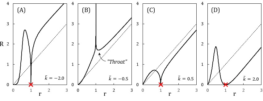
Figure 1: $R$ vs $r$ for the special Buchdahl-inspired metric; $r_{\text{s}}=1$. Panel (B), representative of $\tilde{k}\in(-1,0)$, yields a minimum for $R(r)$ and corresponds to a wormhole.

In terms of $x:=1-\frac{r_{\text{s}}}{r}\in\mathbb{R}$, the special Buchdahl-inspired metric becomes

$$ds^{2} =-\text{sgn}(x)\left|x\right|^{\tilde{k}+1}dt^{2}+\zeta^{4}r_{\text{s}}^{2}\frac{\text{sgn}(x)\left|x\right|^{\tilde{k}+2\zeta-3}}{(1-\text{sgn}(x)\left|x\right|^{\zeta})^{4}}dx^{2}$$

$$\ \ \ \ \ \ \ \ +\zeta^{2}r_{\text{s}}^{2}\frac{\left|x\right|^{\tilde{k}+\zeta-1}}{(1-\text{sgn}(x)\left|x\right|^{\zeta})^{2}}d\Omega^{2}$$ (30)

The areal radius in the class is

$$R=\zeta r_{\text{s}}\frac{\left|x\right|^{\frac{1}{2}(\tilde{k}+\zeta-1)}}{1-\text{sgn}(x)\left|x\right|^{\zeta}}$$ (31)

For the exterior:

$$\frac{dR}{dr} =\frac{\zeta r_{\text{s}}^{2}}{2r^{2}}\frac{x^{\frac{1}{2}(\tilde{k}+\zeta-3)}}{\left(1-x^{\zeta}\right)^{2}}\left[(\tilde{k}-1+\zeta)-(\tilde{k}-1-\zeta)x^{\zeta}\right]$$ (32)

which would have an acceptable root

$$x_{\text{ext}}=\left(\frac{\tilde{k}-1+\sqrt{1+3\tilde{k}^{2}}}{\tilde{k}-1-\sqrt{1+3\tilde{k}^{2}}}\right)^{\frac{1}{\sqrt{1+3\tilde{k}^{2}}}}\in(0,1)$$ (33)

if $\tilde{k}\in(-1,0)$.

For the interior:

$$\frac{dR}{dr} =-\frac{\zeta r_{\text{s}}^{2}}{2r^{2}}\frac{(-x)^{\frac{1}{2}(\tilde{k}+\zeta-3)}}{\left(1+(-x)^{\zeta}\right)^{2}}\left[(\tilde{k}-1+\zeta)+(\tilde{k}-1-\zeta)(-x)^{\zeta}\right]$$ (34)

which would have an acceptable root

$$x_{\text{int}}=-\left(-\frac{\tilde{k}-1+\sqrt{1+3\tilde{k}^{2}}}{\tilde{k}-1-\sqrt{1+3\tilde{k}^{2}}}\right)^{\frac{1}{\sqrt{1+3\tilde{k}^{2}}}}\in(-\infty,0)$$ (35)

if $\tilde{k}\in(-\infty,1)\cup(0,+\infty)$.

The behavior of $R$ as a function of $r$ is shown in 1. Panel (B) is representative of $\tilde{k}\in(-1,0)$ exhibits a minimum for $R(r)$ in the exterior.

We shall bring the metric above to the Morris-Thorne ansatz (MorrisThorne-1988-2, )

$$ds^{2}=-e^{2\Phi(R)}dt^{2}+\frac{dR^{2}}{1-\frac{b(R)}{R}}+R^{2}d\Omega^{2}$$ (36)

If we focus on the “exterior” region alone, then $(x\in(0,1))$

$$ds^{2}=-x^{\tilde{k}+1}dt^{2}+\zeta^{4}r_{\text{s}}^{2}\frac{x^{\tilde{k}+2\zeta-3}}{(1-x^{\zeta})^{4}}dx^{2}+\zeta^{2}r_{\text{s}}^{2}\frac{x^{\tilde{k}+\zeta-1}}{(1-x^{\zeta})^{2}}d\Omega^{2}$$ (37)

For the exterior, viz. $x\in(0,1)$, let us make a further coordinate transformation

$$y:=x^{\zeta}\in(0,1)$$ (38)

and denoting $A:=\frac{\tilde{k}+1}{\zeta}$ and $B:=\frac{\tilde{k}-1}{\zeta}$ (again, $\zeta=\sqrt{1+3\tilde{k}^{2}}$)

$$ds^{2} =-y^{A}dt^{2}+\left(\zeta\,r_{\text{s}}\right)^{2}\frac{y^{B}}{(1-y)^{2}}\left[\frac{dy^{2}}{(1-y)^{2}}+y\,d\Omega^{2}\right]$$ (39)

In summary, the areal radius is defined as

$$R=\zeta\,r_{\text{s}}\frac{y^{\frac{B+1}{2}}}{1-y}$$ (40)

The redshift function and the shape function are given by, respectively,

$$e^{2\Phi(R)} =y^{A},$$ (41)

$$1-\frac{b(R)}{R} =\frac{(1-y)^{4}}{\zeta^{2}r_{\text{s}}^{2}y^{B}}\left(\frac{dR}{dy}\right)^{2}$$ (42)

$$=\frac{1}{4y}\left[(B-1)y-(B+1)\right]^{2}$$ (43)

for the region $y\geqslant y_{*}$ where

$$y_{*}=\frac{B+1}{B-1}$$ (44)

corresponds to $x_{ext}$ in Eq. (33).

The four Morris-Thorne constraints

In the exterior, $r>r_{\text{s}}$, hence $x\in(0,1)$, taking derivative of Eq. (31):

$$\frac{dR}{dy}=\frac{\zeta\,r_{\text{s}}y^{\frac{B-1}{2}}}{2(1-y)^{4}}\left[(B+1)-(B-1)y\right]$$ (45)

The equation $\frac{dR}{dx}=0$ has a single root at

$$y_{*}=\frac{B+1}{B-1}$$ (46)

This root is acceptable, viz. $y_{*}\in(0,1)$ if

$$B<-1\ \ \ \text{or}\ \ \ -1<\tilde{k}<0$$ (47)

The minimum

$$R_{*}=\frac{\zeta\,r_{\text{s}}}{2}(1-B)^{\frac{1-B}{2}}(-1-B)^{\frac{1+B}{2}}$$ (48)

Constraint #1.—The redshift function $\Phi(R)$ (given in (41)) be finite everywhere (hence no horizon).

Constraint #2.—Minimum value of the $R$-coordinate, i.e. at the throat of the wormhole, $R_{*}$ being the minimum value of $R$, given in Eq. (48).

Constraint #3.—Finiteness of the proper radial distance, i.e. $b(R)/R\leq 1$ (for $R\geq R_{*}$) throughout the space. The equality sign holds only at the throat. This is required in order to ensure the finiteness of the proper radial distance $l(R)$ given in (55) where the ± signs refer to the two asymptotically flat regions which are connected by the wormhole. Note that the condition $b(R)/R\leq 1$ assures that the metric component $g_{RR}$ does not change its sign for any $R\geq R_{*}$.

Constraint #4.—Asymptotic flatness condition, i.e. as $l\rightarrow\pm\infty$ (or equivalently, $R\rightarrow\infty$ or $r\rightarrow\infty$ or $x\rightarrow 1^{-}$) then $b(R)/R\rightarrow 0$.

Embedding

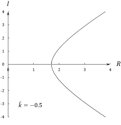
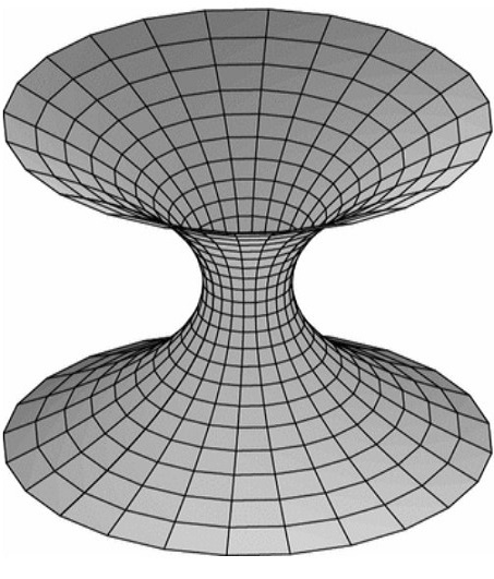
Figure 2: Proper radial distance (upper panel) and embedding diagram (lower panel).

                    

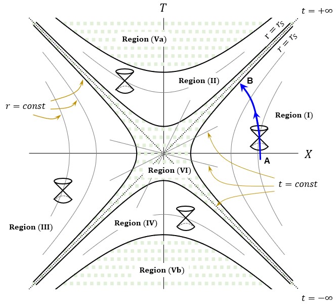
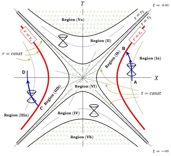
Figure 3: $\ \zeta-$Kruskal-Szekeres diagrams for the asymptotically flat Buchdahl-inspired spacetimes for $\tilde{k}\in(-\infty,-1)\cup(0,+\infty)$ (the case of naked singularity, shown in left panel) and for $\tilde{k}\in(-1,0)$ (the case of wormhole, shown in right panel). Left panel: On the infalling radial timelike trajectory (blue line), a particle in Region (I) eventually hits the naked singularity, $r=r_{\text{s}}$.   Right panel: The wormhole “throat” is depicted by the red lines, which further split Region (I) into (Ia) and (Ib), and Region (III) into (IIIa) and (IIIb). On the radial trajectory $A\rightarrow B\rightarrow C\rightarrow D$, a particle in Region (Ia) first enters the wormhole mouth at point B (hence, an infalling motion) then escape into Region (IIIa) by emerging at the other mouth at point C (hence, on outgoing motion). As the two red lines are “glued” together to form a wormhole that connects Region (Ia) and Region (IIIa), the two opposite points B and C represent the same spacetime event.

With $y_{*}$ defined in Eq. (46), the shape function in Eq. (43) is

$$1-\frac{b(R)}{R}=\frac{(B-1)^{2}}{4y}\left(y-y_{*}\right)^{2}\geq 0$$ (49)

In the embedding diagram, the MT ansatz

$$ds^{2}=-e^{2\Phi(R)}dt^{2}+\left(1+\left(\frac{dz}{dR}\right)^{2}\right)dR^{2}+R^{2}d\Omega^{2}$$ (50)

yields

$$\frac{dz}{dR} =\pm\frac{1}{\sqrt{\frac{R}{b(R)}-1}}=\pm\frac{\sqrt{b(R)/R}}{\sqrt{1-b(R)/R}}$$ (51)

$$=\pm\frac{\sqrt{4y-(B-1)(y-y_{*})^{2}}}{(B-1)(y-y_{*})}$$ (52)

Obviously $dz/dR$ diverges at $y=y_{*}$, meaning that in the embedding diagram (the lower panel of Fig. 2), $z(R)$ is vertical at $y=y_{*},$the “throat” of the wormhole. The function $z(R)$ is a combination of Appell hypergeometric functions that is not particularly illuminating and hence will not be produced here.

Nevertheless, the proper radial distance is simpler to obtain:

$$l(R) =\pm\int_{R_{*}}^{R}\frac{dR}{\sqrt{1-\frac{b(R)}{R}}}$$ (53)

$$=\pm\zeta\,r_{\text{s}}\int_{y_{*}}^{y}dy\frac{y^{\frac{B}{2}}}{(1-y)^{2}}$$ (54)

$$=\pm\frac{\zeta\,r_{\text{s}}}{1+B/2}\times\biggl{[}y^{1+B/2}\,_{2}F_{1}\Bigl{(}2,1+B/2;2+B/2;y\Bigr{)}$$

$$\ \ \ \ \ \ \ \ \ \ \ -y_{*}^{1+B/2}\,{}_{2}F_{1}\Bigl{(}2,1+B/2;2+B/2;y_{*}\Bigr{)}\biggr{]}$$ (55)

As an example, the upper panel of Fig. 2 plots the proper radial distance for $\tilde{k}=-0.5$, viz. $B\approx-1.134$, $y_{*}\approx 0.0628$, $r_{*}\approx 1.14\,r_{\text{s}}$, $R_{*}\approx 1.7\,r_{\text{s}}$. A “throat” is manifest at $R=R_{*}$.

In the range of $\tilde{k}\in(-\infty,-1)\cup(0,+\infty)$, The Kretschmann invariant diverges at $y=0$ (i.e., $r=r_{\text{s}}$), indicating a physical singularity on the interior-exterior boundary, $y=0$. As a result, the spacetime is not geodesically complete, and the geodesics terminate at the physical singularity. The $\zeta-$Kruskal-Szekeres (KS) diagram previously constructed in Ref.  (Nguyen-2023-Lambda0, ) is reproduced in Fig.  3 here for the reader’s convenience. In the left panel of Fig.  3, we also show the radial infalling motion of a massive particle along the trajectory $A\rightarrow B$, with the particle eventually hitting the physical singularity, represented by point $B$ on the interior-exterior boundary.

In the range of $\tilde{k}\in(-1,0)$, the Kretschmann invariant likewise diverges at $y=0$ (i.e., $r=r_{\text{s}}$), indicating a physical singularity on the interior-exterior boundary, $y=0$. However, since the areal radius possesses a minimum value at $y_{*}=\frac{B+1}{B-1}\in(0,\,1)$, we can generate a wormhole solution by “gluing” the region $y_{*}\leq y<1$ (corresponding to $r_{*}\leq r<+\infty$ as shown in Panel (B) of Fig. 1, with $r_{*}=\frac{r_{\text{s}}}{1-y_{*}^{1/\zeta}}>r_{\text{s}}$) with its symmetric counterpart (also in the region $y_{*}\leq y<1$) in the $\zeta-$KS diagram. The right panel of Fig.  3 shows how this is done. The wormhole “throat” is represented by the two red lines, $r=r_{*}$, which further split Region (I) into (Ia) and (Ib), and Region (III) into (IIIa) and (IIIb). That is to say, we are connecting an asymptotically flat exterior sheet (i.e., Region (Ia)) with another asymptotically flat exterior sheet (i.e., Region (IIIa)), which are mirror images of each another with respect to a sign flip $(T,X)\leftrightarrow(-T,-X)$ in their $\zeta-$KS coordinates.

In this construction, both the upper and lower sheets of the wormhole correspond to $r_{*}\leq r<+\infty$ and they approach asymptotic flatness at spatial infinity. The two sheets are smoothly connected at the “throat” at $y=y_{*}$, where $z(R)$ becomes vertical, hence ensuring a smooth connection. The upper and lower sheets are distinguished by the $\pm$ sign in the proper length parameter $l$, per Eq. (55), which runs continuously from $-\infty$ to $\infty$ as a traveler moves from the lower sheet of the wormhole to the upper one.

In the right panel of Fig.  3, the radial infalling motion of a massive particle is depicted by the trajectory $A\rightarrow B$ in Region (Ia), with $B$ lying on the “throat”. The particle then emerges at point $C$ (which also lies on the “throat” and is opposite to point $B$ on the $\zeta-$KS diagram) then continue on the path $C\rightarrow D$ in Region (IIIa). Note that points $B$ and $C$ represent the same spacetime event.

Violation of the Weak Energy Condition

Formally, the geometric form for the Weak Energy Condition requires that $G_{\mu\nu}t^{\mu}t^{\nu}\geq 0$ for every future-pointing timelike vector $t^{\mu}$; e.g., see Ref.  (Koutou, ). In particular, $G_{00}\geq 0$.

The special Buchdahl-inspired metric has the $00-$component of the Einstein tensor

$$G_{00}=\frac{\tilde{k}(\tilde{k}+1)}{2r_{\text{s}}^{2}\zeta^{4}}\frac{\left[1-\text{sgn}\left(1-\frac{r_{\text{s}}}{r}\right)\left|1-\frac{r_{\text{s}}}{r}\right|^{\zeta}\right]^{4}}{\left|1-\frac{r_{\text{s}}}{r}\right|^{2(\zeta-1)}}$$ (56)

For $\tilde{k}\in(-1,0)$, the exterior region exhibits a wormhole “throat” as can be seen in Panel (B) of Fig. 1. At the same time, $G_{00}<0\ \ \forall r$ for $\tilde{k}\in(-1,0)$, thus violating the Weak Energy Condition.

As Morris and Thorne envisioned (MorrisThorne-1988-1, ), in a traversable wormhole, light rays that enter it at one mouth then reemerge at its other mouth have a cross-sectional area initially decreasing and then increasing. In order for this phenomenon to occur, there necessarily be some “gravitational repulsion” near the “throat”, exerting influence on the light rays. In Eq. (56), the magnitude of $G_{00}$ monotonically increases as one approaches the interior-exterior boundary, $r=r_{\text{s}}$. For $\tilde{k}\in(-1,0)$, the negative and dominant $G_{00}$ component thus acts like gravitational repulsion. We expect that it could leave signatures, distinguishing a wormhole from a black hole (distinguish, ).

Simultaneously, the interior-exterior boundary is a set of naked singularities. Consequently, the spacetime for $\tilde{k}\in(-1,0)$ accommodates both a wormhole connecting two asymptotically flat exterior sheets (viz. Regions (Ia) and (IIIa) in Fig.  3) and a set of naked singularities (belonging to Regions (Ib) and (IIIb)), thereby representing a non-trivial geometrical structure in this situation.

As mentioned in the concluding remark of Section II, the right hand side of Eq.  (10) corresponds to a “quasi” energy-momentum tensor, defined as (modulo a multiplicative constant)

$$T_{\text{$\mu\nu$}}:=\mathcal{R}^{-1}\nabla_{\mu}\nabla_{\nu}\mathcal{R}$$ (57)

It was shown in Ref.  (Nguyen-2023-Nontrivial, ) that despite the vanishing Ricci scalar throughout spacetime, this “quasi” energy-momentum tensor remains well-defined and is identical to the $G_{00}$ component presented in Eq. (56). It effectively serves as a surrogate to exotic matter required to sustain a wormhole.

V Conclusion

In a previous work (Nguyen-2023-Lambda0, ), we derived a special Buchdahl-inspired metric that describes asymptotically flat spacetimes in pure $\mathcal{R}^{2}$ gravity. This metric, expressed in a closed analytical form, enabled us to construct a Kruskal-Szekeres diagram representing the maximal analytic extension for the metric. The Buchdahl parameter $\tilde{k}$ in the metric is a new parameter that reflects the higher-derivative nature of the pure $\mathcal{R}^{2}$ action.

In this paper, we present several additional advancements. Firstly, we describe two additional representations of the metric. Secondly, we examine the metric within the framework of the Morris-Thorne ansatz. For values of $\tilde{k}$ falling within the ranges $(-\infty,-1)$ and $(0,+\infty)$, the interior-exterior boundary constitutes a naked singularity. However, for the range $\tilde{k}\in(-1,0)$, the areal radius has a minimum value in exterior region. Despite the geodesic incompleteness of the solution in this situation, where geodesics terminate on the singularity, it is possible to shield the singularity by removing the region of space neighboring the singularity and gluing the Kruskal-Szekeres symmetric copy of the remaining space region to that same region. The Morris-Thorne-Buchdahl wormhole constructed this way consists of a pair of asymptotically flat spacetime sheets connected at a “throat” that allows two-way passage.

Thirdly, we find that when a wormhole is formed, that is, when $\tilde{k}\in(-1,0)$, the Weak Energy Condition is formally violated, even though no exotic matter is in presence. Therefore, pure $\mathcal{R}^{2}$ theory can support a wormhole without the need for truly exotic matter in the energy-momentum tensor or complicated ingredients in the gravitation sector such as torsion, non-metricity, or non-locality. Our work opens up new avenues for exploring the fascinating properties of wormholes and naked singularities in higher-derivative gravity theories. For wormholes and naked singularities of quadratic relativity, all known potential astrophysical observations, including light deflection, precession, shadow, and quasi-periodic oscillations are the subjects of a future investigation (future, ) and cannot be carried out in this work.

Another important question, even more important than all that has been said, is the stability of the wormhole discussed in this work. Stability analysis is a more involved issue (st1, ; st2, ; s1, ; s2, ; s3, ) as this necessitates to perform a perturbation analysis of the metric, which will make the subject of another subsequent paper. However, based on the generic analysis made in (s4, ) the wormhole is likely to be stable.

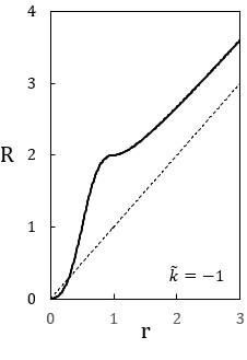
Figure 4: $R$ vs $r$ of the special Buchdahl-inspired metric for $\tilde{k}=-1$, $r_{\text{s}}=1$.

—————–$\infty$—————–

Appendix A  The borderline case of $\tilde{k}=-1$

For completeness, we shall briefly examine the $\tilde{k}=-1$ case, viz. $\zeta=2$. With $x:=1-\frac{r_{\text{s}}}{r}$, from (31), the areal radius is

$$R=\frac{2r_{\text{s}}}{1-\text{sgn}(x)x^{2}}=\frac{2r_{\text{s}}}{1-\text{sgn}\left(1-\frac{r_{\text{s}}}{r}\right)\left(1-\frac{r_{\text{s}}}{r}\right)^{2}}$$ (58)

which is a monotonic increasing function for $r\in\mathbb{R}^{+}$ and $R(r=r_{\text{s}})=2r_{\text{s}}$, as shown in Fig. 4. In this coordinate, the metric (30) becomes

$$ds^{2}=-\text{sgn}\left(1-\frac{2r_{\text{s}}}{R}\right)dt^{2}+\frac{dR^{2}}{1-\frac{2r_{\text{s}}}{R}}+R^{2}\,d\Omega^{2}$$ (59)

which differs from the Schwarzschild metric by the $g_{tt}$ component. The equations of motion (EOM) in the exterior, viz. $R>2r_{\text{s}}$, are

$$\frac{d}{d\tau}\left(g_{\sigma\lambda}\frac{dx^{\lambda}}{d\tau}\right)=\frac{1}{2}\partial_{\sigma}g_{\mu\nu}\frac{dx^{\mu}}{d\tau}\frac{dx^{\nu}}{d\tau}$$ (60)

or (with $\mathcal{E}$ and $l$ being two constants of motions, the dot denoting derivative with respect to $\tau$, and restricting to the $\theta=\pi/2$ plane)

$$\dot{t} =\mathcal{E}\ \ \ \ \ \text{for }\sigma=\lambda=0$$ (61)

$$\dot{\varphi} =\frac{l}{R^{2}}\ \ \ \ \ \text{for }\sigma=\lambda=2$$ (62)

subject to a constraint

$$-\dot{t}^{2}+\frac{\dot{R}^{2}}{1-\frac{2r_{\text{s}}}{R}}+R^{2}\dot{\varphi}^{2} =f=\begin{cases}\ \ 0&\text{for null geodesics}\\ -1&\text{for timelike geodesics}\end{cases}$$ (63)

We subsequently get

$$\dot{R}^{2} =\left(1-\frac{2r_{\text{s}}}{R}\right)\left(f+\mathcal{E}^{2}-\frac{l^{2}}{R^{2}}\right)$$ (64)

$$=f+\mathcal{E}^{2}-\frac{l^{2}}{R^{2}}-\frac{2r_{\text{s}}(f+\mathcal{E}^{2})}{R}+\frac{2r_{\text{s}}l^{2}}{R^{3}}$$ (65)

and

$$\ddot{R}=\frac{r_{\text{s}}(f+\mathcal{E}^{2})}{R^{2}}+l^{2}\left(\frac{1}{R^{3}}-\frac{3r_{\text{s}}}{R^{4}}\right)$$ (66)

For a massive object $(f=-1)$:

$$\ddot{R}=-(1-\mathcal{E}^{2})\frac{r_{\text{s}}}{R^{2}}+l^{2}\left(\frac{1}{R^{3}}-\frac{3r_{\text{s}}}{R^{4}}\right)$$ (67)

Compared with the EOM in Schwarzschild $\ddot{R}=-\frac{r_{\text{s}}}{2R^{2}}+l^{2}\left(\frac{1}{R^{3}}-\frac{3r_{\text{s}}}{2R^{4}}\right)$, the only modification is the Newtonian potential being “renormalized” by $(1-\mathcal{E}^{2})$ and thus acting like “repulsive” force if $\mathcal{E}^{2}>1$. It is worth mentioning that this is a partial result of much wider conclusions drawn in (future, ) for any $\tilde{k}$, among which the velocity-dependent acceleration for massive objects.

References

- (1) M. S. Morris and K. S. Thorne, Wormholes in spacetime and their for interstellar travel: A tool for teaching general relativity, Am. J. Phys. 56, 5 (1988)
- (2) M. S. Morris, K. S. Thorne, and U. Yurtsever, Wormholes, Time Machines, and the Weak Energy Condition, Phys. Rev. Lett. 61, 1446 (1988)
- (3) T. Damour and S. N. Solodukhin, Wormholes as black hole foils, Phys. Rev. D 76, 024016 (2007), arXiv:0704.2667 [gr-qc]
- (4) C. Bambi, Can the supermassive objects at the centers of galaxies be traversable wormholes? The first test of strong gravity for mm/sub-mm very long baseline interferometry facilities, Phys. Rev. D 87, 107501 (2013), arXiv:1304.5691 [gr-qc]
- (5) M. Azreg-Aïnou, Confined-exotic-matter wormholes with no gluing effects - Imaging supermassive wormholes and black holes, JCAP 07, 037 (2015), arXiv:1412.8282 [gr-qc]
- (6) V. Dzhunushaliev, V. Folomeev, B. Kleihaus, and J. Kunz, Can mixed star-plus-wormhole systems mimic black holes?, JCAP 08, 030 (2016), arXiv:1601.04124 [gr-qc]
- (7) V. Cardoso, E. Franzin, and P. Pani, Is the Gravitational-Wave Ringdown a Probe of the Event Horizon?, Phys. Rev. Lett. 116, 171101 (2016), arXiv:1602.07309 [gr-qc]
- (8) R. A. Konoplya and A. Zhidenko, Wormholes versus black holes: quasinormal ringing at early and late times, JCAP 12, 043 (2016), arXiv:1606.00517 [gr-qc]
- (9) K. K. Nandi, R. N. Izmailov, A. A. Yanbekov, and A. A. Shayakhmetov, Ring-down gravitational waves and lensing observables: How far can a wormhole mimic those of a black hole?, Phys. Rev. D 95, 104011 (2017), arXiv:1611.03479 [gr-qc]
- (10) P. Bueno, P. A. Cano, F. Goelen, T. Hertog, and B. Vercnocke, Echoes of Kerr-like wormholes, Phys. Rev. D 97, 024040 (2018), arXiv:1711.00391 [gr-qc]
- (11) J. G. Cramer, R. L. Forward, M. S. Morris, M. Visser, G. Benford, and G. A. Landis, Natural wormholes as gravitational lenses, Phys. Rev. D 51, 3117 (1995), arXiv:astro-ph/9409051
- (12) P. G. Nedkova, V. K. Tinchev, and S. S. Yazadjiev, Shadow of a rotating traversable wormhole, Phys. Rev. D 88, 124019 (2013), arXiv:1307.7647 [gr-qc]
- (13) T. Harko, Z. Kovacs, and F. S. N. Lobo, Thin accretion disks in stationary axisymmetric wormhole spacetimes, Phys. Rev. D 79, 064001 (2009), arXiv:0901.3926 [gr-qc]
- (14) E. Deligianni, J. Kunz, P. Nedkova, S. Yazadjiev, and R. Zheleva, Quasiperiodic oscillations around rotating traversable wormholes, Phys. Rev. D 104, 024048 (2021), arXiv:2103.13504 [gr-qc]
- (15) V. De Falco, M. De Laurentis, and S. Capozziello, Epicyclic frequencies in static and spherically symmetric wormhole geometries, Phys. Rev. D 104, 024053 (2021), arXiv:2106.12564 [gr-qc]
- (16) F. Duplessis and D. A. Easson, Exotica ex nihilo: Traversable wormholes non-singular black holes from the vacuum of quadratic gravity, Phys. Rev. D 92, 043516 (2015), arXiv:1506.00988 [gr-qc]
- (17) J. B. Dent, D. A. Easson, T. W. Kephart, and S. C. White, Stability Aspects of Wormholes in Gravity, Int. J. Mod. Phys. D 26, 1750117 (2017), arXiv:1608.00589 [gr-qc]
- (18) K. Jusufi, A. Övgün, A. Banerjee, İ. Sakallı, Gravitational lensing by wormholes supported by electromagnetic, scalar, and quantum effects, Eur. Phys. J. Plus 134, 428 (2019), arXiv:1802.07680 [gr-qc]
- (19) İ. Sakallı, A. Övgün, Gravitinos tunneling from traversable Lorentzian wormholes, Astrophys Space Sci 359, 32 (2015), arXiv:1506.00599 [gr-qc]
- (20) V. De Falco, E. Battista, S. Capozziello, and M. De Laurentis, Reconstructing wormhole solutions in curvature based Extended Theories of Gravity, Eur. Phys. J. C 81, 157 (2021), arXiv:2102.01123 [gr-qc]
- (21) X. Y. Chew, B. Kleihaus, and J. Kunz, Spinning Wormholes in Scalar-Tensor Theory, Phys. Rev. D 97, 064026 (2018), arXiv:1802.00365 [gr-qc]
- (22) A. Övgün, K. Jusufi, and İ. Sakallı, Exact traversable wormhole solution in bumblebee gravity, Phys. Rev. D 99, 024042 (2019), arXiv:1804.09911 [gr-qc]
- (23) M. S. Churilova, R. A. Konoplya, Z. Stuchlík, and A. Zhidenko, Wormholes without exotic matter: quasinormal modes, echoes and shadows, JCAP 10, 010 (2021), arXiv:2107.05977 [gr-qc]
- (24) G. Clément and D. Gal’tsov, Rotating traversable wormholes in Einstein–Maxwell theory, Phys. Lett. B 838, 137677 (2023), arXiv:2210.08913 [gr-qc]
- (25) A. G. Agnese and M. La Camera, Wormholes in the Brans-Dicke theory of gravitation, Phys. Rev. D 51, 2011 (1995)
- (26) A. G. Agnese and M. La Camera, Schwarzschild metrics, quasi-universes and wormholes, in Sidharth, B. G., Altaisky, M. V. (eds) Frontiers of Fundamental Physics 4. Springer, Boston, MA, https://doi.org/10.1007/978-1-4615-1339-1_18, arXiv:astro-ph/0110373
- (27) M. Campanelli and C. Lousto, Are Black Holes in Brans-Dicke Theory precisely the same as in General Relativity?, Int. J. Mod. Phys. D 2, 451 (1993), arXiv:gr-qc/9301013
- (28) L. Vanzo, S. Zerbini, and V. Faraoni, Campanelli-Lousto and veiled spacetimes, Phys. Rev. D 86, 084031 (2012), arXiv:1208.2513 [gr-qc]
- (29) A. A. Sen and R. J. Scherrer, The weak energy condition and the expansion history of the Universe, Phys. Lett. B 659, 457 (2008), arXiv:0703416 [astro-ph]
- (30) J. Santos, J. S. Alcaniz, and M. J. Rebouşas, Energy conditions and supernovae observations, Phys. Rev. D 74 (2006) 067301, arXiv:0608031 [astro-ph]
- (31) R. M. Wald, Asymptotic behavior of homogeneous cosmological models in the presence of a positive cosmological constant, Phys. Rev. D 28 (1983) 2118
- (32) G. J. Galloway, The lorentzian splitting theorem without the completeness assumption, Journal of differential geometry 29, 373 (1983)
- (33) C. Barceló and M. Visser, Scalar fields, energy conditions and traversable wormholes, Class. Quantum Grav. 17, 3843 (2000), arXiv:0003025 [gr-qc]
- (34) L. H. Ford and T. A. Roman, Classical scalar fields and the generalized second law, Phys. Rev. D 64, 024023 (2001), arXiv:0009076 [gr-qc]
- (35) A. Borde and A. Vilenkin, Violation of the weak energy condition in inflating spacetimes, Phys. Rev. D 56, 717 (1997), arXiv:9702019 [gr-qc]
- (36) S. Kar, N. Dadhich, and M. Visser, Quantifying energy condition violations in traversable wormholes, Pramana - J. Phys. 63, 859 (2004), arXiv:0405103 [gr-qc]
- (37) E. Curiel, A Primer on Energy Conditions in D. Lehmkuhl, G. Schiemann, E. Scholz (eds), Towards a Theory of Spacetime Theories. Einstein Studies, vol. 13, Birkhäuser, New York, NY (2017)
- (38) H. A. Buchdahl, On the Gravitational Field Equations Arising from the Square of the Gaussian Curvature, Nuovo Cimento 23, 141 (1962), https://link.springer.com/article/10.1007/BF02733549
- (39) W. Nelson, Static solutions for fourth order gravity, Phys. Rev. D 82, 104026 (2010), arxiv:1010.3986 [gr-qc]
- (40) H. Lü, A. Perkins, C. N. Pope, and K. S. Stelle, Black holes in higher-derivative gravity, Phys. Rev. Lett. 114, 171601 (2015), arxiv:1502.01028 [hep-th]; H. Lü, A. Perkins, C. N. Pope, and K. S. Stelle, Spherically symmetric solutions in higher-derivative gravity, Phys. Rev. D 92, 124019 (2015), arXiv:1508.00010 [hep-th]
- (41) A. Kehagias, C. Kounnas, D. Lüst, and A. Riotto, Black hole solutions in gravity, J. High Energy Phys. 05, 143 (2015), arXiv:1502.04192 [hep-th]
- (42) V. Pravda, A. Pravdová, J. Podolský, and R. Švarc, Exact solutions to quadratic gravity, Phys. Rev. D 95, 084025 (2017), arXiv:1606.02646 [gr-qc]; J. Podolský, R. Švarc, V. Pravda, and A. Pravdová, Explicit black hole solutions in higher-derivative gravity, Phys. Rev. D 98, 021502 (2018), arXiv:1806.08209 [gr-qc]
- (43) M. Gürses, T.Ç. Şişman, and B. Tekin, New exact solutions of quadratic curvature gravity, Phys. Rev. D 86, 024009 (2012); arXiv:1204.2215 [hep-th]
- (44) E. Alvarez, J. Anero, S. Gonzalez-Martin, and R. Santos-Garcia, Physical content of quadratic gravity, Eur. Phys. J. C 78, 794 (2018), arXiv:1802.05922 [hep-th]
- (45) K. S. Stelle, Renormalization of higher-derivative quantum gravity, Phys. Rev. D 16, 953 (1977); K. S. Stelle, Classical Gravity with Higher Derivatives, Gen. Rel. Grav. 9, 353 (1978)
- (46) V. P. Frolov and I. L. Shapiro, Black Holes in Higher Dimensional Gravity Theory with Quadratic in Curvature corrections, Phys. Rev. D 80, 044034 (2009), arXiv:0907.1411 [gr-qc]
- (47) S. Murk, Physical black holes in fourth-order gravity, Phys. Rev. D 105, 044051 (2022), arXiv:2110.14973 [gr-qc]
- (48) T. Clifton, Spherically Symmetric Solutions to Fourth-Order Theories of Gravity, Class. Quant. Grav. 23, 7445 (2006), arXiv:gr-qc/0607096
- (49) M. Rinaldi, On the equivalence of Jordan and Einstein frames in scale-invariant gravity, Eur. Phys. J. Plus 133, 408 (2018), arXiv:1808.08154 [gr-qc]
- (50) J. F. Donoghue and G. Menezes, Gauge assisted quadratic gravity: A framework for UV complete quantum gravity, Phys. Rev. D 97, 126005 (2018), arXiv:1804.04980 [hep-th]
- (51) P. G. Ferreira and O. J. Tattersall, Scale invariant gravity and black hole ringdown, Phys. Rev. D 101, 024011 (2020), arXiv:1910.04480 [gr-qc]
- (52) H. K. Nguyen, Beyond Schwarzschild-de Sitter spacetimes: I. A new exhaustive class of metrics inspired by Buchdahl for pure gravity in a compact form, Phys. Rev. D 106, 104004 (2022), arXiv:2211.01769 [gr-qc]
- (53) H. K. Nguyen, Beyond Schwarzschild-de Sitter spacetimes: II. An exact non-Schwarzschild metric in pure gravity and new anomalous properties of spacetimes, Phys. Rev. D 107, 104008 (2023), arXiv:2211.03542 [gr-qc]
- (54) H. K. Nguyen, Beyond Schwarzschild-de Sitter spacetimes: III. A perturbative vacuum with non-constant scalar curvature in gravity, Phys. Rev. D 107, 104009 (2023), arXiv:2211.07380 [gr-qc]
- (55) H. K. Nguyen, Non-triviality of asymptotically flat Buchdahl-inspired metrics in pure gravity, arXiv:2305.12037 [gr-qc]
- (56) M. Azreg-Aïnou and H. K. Nguyen, A stationary axisymmetric vacuum solution for pure gravity, arXiv:2304.08456 [gr-qc]
- (57) H. K. Nguyen and M. Azreg-Aïnou, Traversable Morris-Thorne-Buchdahl wormholes in quadratic gravity, arXiv:2305.04321 [gr-qc]
- (58) A. Edery and Y. Nakayama, Restricted Weyl invariance in four-dimensional curved spacetime, Phys. Rev. D 90, 043007 (2014), arXiv:1406.0060 [hep-th]
- (59) R. P. Woodard, Avoiding Dark Energy with Modifications of Gravity, Lect. Notes Phys. 720, 403 (2007), arXiv:astro-ph/0601672; R. P. Woodard, Ostrogradsky’s theorem on Hamiltonian instability, Scholarpedia 10, 32243 (2015), arXiv:1506.02210 [hep-th]
- (60) L. Alvarez-Gaume, A. Kehagias, C. Kounnas, D. Lüst, and A. Riotto, Aspects of Quadratic Gravity, Fortsch. Phys. 64, 176 (2016), arXiv:1505.07657 [hep-th]
- (61) H. K. Nguyen, Emerging Newtonian potential in pure gravity on a de Sitter background, arXiv:2306.03790 [gr-qc]
- (62) H. K. Nguyen and M. Azreg-Aïnou, New insights into Weak Energy Condition and wormholes in Brans-Dicke gravity, arXiv:2305.15450 [gr-qc]
- (63) E-A. Kontou and K. Sanders, Energy conditions in general relativity and quantum field theory, Class. Quantum. Grav. 37 (2020), 193001, arXiv:2003.01815 [gr-qc]
- (64) N. Tsukamoto, T. Harada, and K. Yajima, Can we distinguish between black holes and wormholes by their Einstein ring systems?, Phys. Rev. D 86, 104062 (2012), arXiv:1207.0047 [gr-qc]; C. Bambi and D. Stojkovic, Astrophysical Wormholes, Universe 7, 136 (2021), arXiv:2105.00881 [gr-qc]
- (65) K. Jusufi, M. Azreg-Aïnou, and M. Jamil, Orbital motions in the special Buchdahl-inspired metric (in preparation)
- (66) M. Azreg-Aïnou, Instability of two-dimensional heterotic stringy black holes, Class. Quantum. Grav. 16 (1999) 245, arXiv:9902005 [gr-qc]
- (67) M. Azreg-Aïnou, G. Clément, C. P. Constantinidis, J. C. Fabris, Electrostatic solutions in Kaluza-Klein theory: geometry and stability, Grav. Cosmol. 6 (2000) 207, arXiv:9911107 [gr-qc]
- (68) K. Bronnikov, S. Bolokhov, A. Makhmudov, and M. Skvortsova, “Trapped ghost” wormholes and regular black holes. The stability problem, Modern Physics of Compact Stars and Relativistic Gravity, 2017, Yerevan
- (69) F. S. N. Lobo, Stability of phantom wormholes, Phys. Rev. D 71 (2005) 124022, arXiv:0506001 [gr-qc]
- (70) D. I. Novikov, A. G. Doroshkevich, I. D. Novikov, and A. A. Shatskii, Semi-permeable wormholes and the stability of static wormholes, Astron. Rep. 53, (2009), 1079 arXiv:0911.4456 [gr-qc]
- (71) K. A. Bronnikov and S. G. Rubin, Black holes, cosmology and extra dimensions, 2nd edition, World Scientific, Singapore, 2022