Yinong Wu¹, Dehui Wang²

Abstract. In the current study, a brand-new SINARS(1) model is proposed for stationary discrete time series defined on $\boldsymbol{Z}$, based on extended binomial distribution and the Pegram’s operator. The model effectively characterizes the series of positive and negative integer values generated after differencing some non-stationary time series. The model’s attributes are addressed. For the parameter estimation of the model, the conditional maximum likelihood method and Yule-Walker method are taken into consideration. And we prove the asymptotic normality of CML method. By using these two methods, we simulate our model comparing with some relevant ones proposed before. The model can deal with positive or negative autocorrelation data. The analysis of the number of differenced daily new cases in Barbados is done using the suggested model.
Key words and phrases: Asymptotic distribution, Skellam distribution, Extended binomial distribution, Pegram’s operator, CMLE.

1 Introduction

It is well fact that modeling count time series has a crucial role in both financial and medical applications. In some cases, some non-stationary time series produces series of positive and negative integer values after differenced. Therefore, the modeling of integer value series is extremely important.There are numerous models used to analyze discrete time series defined on $\boldsymbol{Z}$. For instance, Andersson and Karlis[8] presented the SINAR process with Skellam innovations (SINARS), which can handle data described on both positive and negative integers. An integer-valued autoregressive process of order $p$ with a signed binomial thinning operator (INARS(p)) was also introduced by Kachour et al.[21], which expanded the order from one to $p$. And as expansion of INARS(p), Zhang et al.[45] proposed INAR(p) process with signed generalized power series thinning operator, which can dealt with negative integer-valued time series. As supplementary, Wang et al.[39] introduced generalized RCINAR(p) process with signed thinning operator. Furthermore, Chesneau and Kachour [12] considered the P-INAR(1) process with Rademacher(p) distribution to deal with data on $\boldsymbol{Z}$.

The ZOIPLINAR(1) model, which was developed by Mohammadi et al.[29] in 2021, is a stationary INAR(1) model with zero-and-one inflated Poisson-Lindley distributed innovations. An integer-valued time series model of order one with an innovation structure of the zero-and-one inflated type is proposed to describe nonnegative data with plenty of zero and one. The analysis of two medical series, including the quantity of fresh COVID-19-infected series from Barbados and data on Poliomyelitis in [30], is then conducted using the zero-and-one-inflated INAR model.

An INAR(1) model based on the combination of Pegram and thinning operators (MPT) with serially dependent innovation was introduced by Shirozhan and Mohammadpour [37], which offered additional flexibility in empirical modeling.

Since the PDINAR model is most used processing series with Skellam marginal distribution, we want to extend it to unconstrained marginal distribution. We integrate the PDINAR model with the Pegram operator based on these studies. The following equation describes the PDINAR(1) time series model: $Z_{t}=\delta S_{\alpha,\theta}\left(Z_{t-1}\right)+\varepsilon_{t},$ where $\delta$ is the sign of autocorrelation, $S_{\alpha,\theta}(Z)$ is extended binomial operator and $\{\varepsilon_{t}\}$ is a sequence of independent and identically Skellam distributed random variables with mean $\theta_{1}-\theta_{2}$ and variance $\theta_{1}+\theta_{2}$. It is proposed by Alzaid and Omair[7] and applied in financial data, Saudi Telecommunication Company (STC) stock and the Electricity stock.

In this paper, we give a new signed integer-valued autoregressive process based on the Pegram’s operator. The remainder of the paper is organized as follows. In this paper, we first show preparation information. Section 2 presents definition and fundamental properties for extended binomial distribution, Skellam distribution and properties of the model we proposed. Section 3 gives conditional maximum likelihood method (CML) and Yuler-Walker method for estimating the unknown parameters. It is shown that CML method is consistent and asymptotically normal. Section 4 reports some simulation results. Section 5 gives applications for the number of new cases in Barbodos. Section 6 shows conclusion of results and prospect work to do. Details of proofs are given in Appendix.

2 Definition and Basic Properties

In this part, we first show the definition of Skellam distribution, afterward we present essential properties for the two distributions and then for the model.

2.1 Skellam Distribution

As it is defined in [20], a random variable $Z$ in $\mathbf{Z}$ has Skellam distribution with parameters $\theta_{1}\geq 0$ and $\theta_{2}\geq 0$ if
$P(Z=z)=e^{-\theta_{1}-\theta_{2}}\left(\frac{\theta_{1}}{\theta_{2}}\right)^{z/2}I_{z}\left(2\sqrt{\theta_{1}\theta_{2}}\right),\quad z=\ldots,-1,0,1,\ldots$
where

$$I_{y}(x)=\left(\frac{x}{2}\right)^{y}\sum_{k=0}^{\infty}\frac{\left(\frac{x^{2}}{4}\right)^{k}}{k!(y+k)!}$$ (1)

is the modified Bessel function of the first kind. For convenience, we use $PD(\theta_{1},\theta_{2})$ to describe Skellam distribution.

Remark 1.

Alzaid et al.[5] showed another equivalent formular of Skellam distribution $P(Z=z)=e^{-\theta_{1}-\theta_{2}}\left(\theta_{1}\theta_{2}\right)^{\max\{0,-z\}}\theta_{1}^{y}{}_{0}\widetilde{F}_{1}\left(|z|+1,\theta_{1}\theta_{2}\right),\quad z=\cdots,-1,0,1,\cdots$

2.2 Extended Binomial Distriution

To consider the orginal definition of EB distribution first proposed by Alzaid and Omair [6] we can let $W\sim PD(\theta_{1},\theta_{2})$, be independent of $R\sim PD(\theta_{3},\theta_{4})$, then the sum $Z=W+R\sim PD(\theta_{1}+\theta_{3},\theta_{2}+\theta_{4})$,
then, the conditional distribution, $W|Z\sim ConditionalPD(z,\theta_{1},\theta_{2},\theta_{3},\theta_{4})$ i.e.,

$$P(W=w|Z=z)=\frac{P(W=w)P(R=z-w)}{P(Z=z)}$$

$$\quad\quad\quad\quad\quad\quad\quad\quad=\frac{\left(\frac{\theta_{1}}{\theta_{1}+\theta_{3}}\right)^{w}{}_{0}^{w}\widetilde{F}_{1}\left(;w+1;\theta_{1}\theta_{2}\right)\left(\frac{\theta_{3}}{\theta_{1}+\theta_{3}}\right)^{z-w}{}_{0}\widetilde{F}_{1}\left(;z-w+1;\theta_{3}\theta_{4}\right)}{{}_{0}\widetilde{F}_{1}\left(;z+1;\left(\theta_{1}+\theta_{3}\right)\left(\theta_{2}+\theta_{4}\right)\right)},$$

$$\quad\quad\quad\quad\quad\quad\quad\quad\quad w=\ldots,-1,0,1,\ldots$$ (2)

By the constraint $\theta_{1}\theta_{4}=\theta_{2}\theta_{3}$ and the following reparametrization:
$z=z$, $p=\frac{\theta_{1}}{\theta_{1}+\theta_{3}}$, $q=1-p$, $\theta=(\theta_{1}+\theta_{3})(\theta_{2}+\theta_{4})$, we derive the EB distribution.

A random variable $X$ in $\mathbf{Z}$ has extended binomial distribution with parameters $0<p<1$, $q=1-p$, $\theta>0$ and $z\in\mathbf{Z}$, denoted by $X\sim EB(z,p,\theta)$ if

$$P(X=x)=\frac{p^{x}q^{z-x}{}_{0}\widetilde{F}_{1}\left(;x+1;p^{2}\theta\right){}_{0}\widetilde{F}_{1}\left(;z-x+1;q^{2}\theta\right)}{{}_{0}\widetilde{F}_{1}(;z+1;\theta)}\qquad x=\ldots,-1,0,1,\ldots$$ (3)

where the regularized hypergeometric function ${}_{0}\widetilde{F}_{1}$ is defined as:

$${}_{0}\widetilde{F}_{1}\left(;y;\theta\right)=\sum_{k=0}^{\infty}\frac{\theta^{k}}{k!\Gamma(y+k)}.$$ (4)

For convenience, we use $EB(z,p,\theta)$ to describe extended binomial distribution.

2.2.1 Extended Binomial Thinning Operator

The extended binomial thinning operator raised by Alzaid and Omair [7] has the following presentation

$$S_{\alpha,\theta}(Z)=(\operatorname{sgn}Z)\sum_{i=1}^{|Z|}Y_{i}+\sum_{i=1}^{W(Z)}B_{i}$$ (5)

where $Y_{i}$ is a sequence of i.i.d.random variables, independent of $B_{i}$, $Z$ and $W(Z)$, such that $P\left(Y_{i}=1\right)=1-P\left(Y_{i}=0\right)=\alpha$, $\left\{B_{i}\right\}$ is a sequence of i.i.d.random variables independent of $Y_{i}$, $Z$ and $W(Z)$ such that
$P\left(B_{i}=1\right)=P\left(B_{i}=-1\right)=\alpha(1-\alpha)$ and $P\left(B_{i}=0\right)=1-2\alpha(1-\alpha)$,
and $W(Z)|Z=z$ is a random variable having Bessel distribution [19] with parameters $(|z|,\theta)$.

Since $\sum_{i=1}^{|Z|}Y_{i}|Z=z\sim\operatorname{\emph{binomial}}(|z|,\alpha)$, $\sum_{i=1}^{W(Z)}B_{i}|Z=z$ has the distribution with characteristic function given by

$$\Phi(t)=\frac{{}_{0}\widetilde{F}_{1}\left(;|z|+1;\theta\left(\alpha(1-\alpha)e^{it}+\alpha(1-\alpha)e^{-it}+1-2\alpha(1-\alpha)\right)\right)}{{}_{0}\widetilde{F}_{1}(;|z|+1;\theta)}.$$ (6)

And it is clear that $S_{\alpha,\theta}(Z)|Z=z\sim EB(z,\alpha,\theta)$.

2.3 Models and Properties

Let us define the stationary MESINAR(1) ${Z_{t}}$ as

$$Z_{t}=\left(\phi,\delta S_{\alpha,\theta}\left(Z_{t-1}\right)\right)*\left(1-\phi,\varepsilon_{t}\right)$$ (7)

where $\delta=1$ or $-1$ decided by the sign of the correlation, the Pegram operator ’*’ mix two independent P and Q with the respective mixing weight of $\phi$ and $1-\phi$, to produce a random variable $Z=(\phi,P)*(1-\phi,Q)$. $\{\varepsilon_{t}\}$ is a sequence of independent and identically Skellam distributed random variables with mean $\theta_{1}-\theta_{2}$ and variance $\theta_{1}+\theta_{2}$.

Since the process is Markovian, the one step transition probability is

$$P(Z_{t}=z_{t}|Z_{t-1}=z_{t-1}) =\phi P\left(\delta S_{\alpha,\theta}(Z_{t-1})=z_{t}\right)+(1-\phi)P(\varepsilon_{t}=z_{t})$$

$$=\phi P\left(S_{\alpha,\theta}(Z_{t-1})=\delta z_{t}\right)+(1-\phi)P(\varepsilon_{t}=z_{t})$$

$$=\phi p^{\delta z_{t}}(1-p)^{z_{t-1}-\delta z_{t}}\frac{{}_{0}\widetilde{F}_{1}(;\delta z_{t}+1;p^{2}\theta){}_{0}\widetilde{F}_{1}(;z_{t-1}-\delta z_{t}+1;(1-p)^{2}\theta)}{{}_{0}\widetilde{F}_{1}(;z_{t-1}+1;\theta)}$$

$$\quad+(1-\phi)e^{-\theta_{1}-\theta_{2}}(\theta_{1}\theta_{2})^{\max(0,-z_{t})}\theta_{1}^{z_{t}}{}_{0}\widetilde{F}_{1}(;|z_{t-1}|+1;\theta_{1}\theta_{2})$$ (8)

The conditional mean is

$$E[Z_{t}|Z_{t-1}]=\phi p\delta Z_{t-1}+(1-\phi)(\theta_{1}-\theta_{2}).$$ (9)

The conditional variance is

$$Var[Z_{t}|Z_{t-1}] =\phi\left(p(1-p)Z_{t-1}+2p(1-p)\theta\frac{{}_{0}\widetilde{F}_{1}(;Z_{t-1}+2;\theta)}{{}_{0}\widetilde{F}_{1}(;Z_{t-1}+1;\theta)}\right)+(1-\phi)(\theta_{1}+\theta_{2})$$

$$\quad+\phi(1-\phi)(p\delta Z_{t-1}-(\theta_{1}-\theta_{2}))^{2}.$$ (10)

The unconditional mean is

$$E[Z_{t}]=\frac{(1-\phi)(\theta_{1}-\theta_{2})}{1-\phi p\delta}.$$ (11)

The unconditional variance is

$$Var[Z_{t}] =\frac{p(1-p)\phi(1-\phi)(\theta_{1}-\theta_{2})}{(1-\phi^{2}p^{2}-(1-\phi)p^{2})(1-\phi p\delta)}-\frac{2\phi(1-\phi)^{3}p\delta(\theta_{1}-\theta_{2})^{2}}{(1-\phi^{2}p^{2}-(1-\phi)p^{2})(1-\phi p\delta)}$$

$$\quad-\frac{(1-\phi)^{2}(\theta_{1}-\theta_{2})^{2}}{(1-\phi p\delta)^{2}}+\frac{2\phi p(1-p)\theta}{(1-\phi^{2}p^{2}-(1-\phi)p^{2})}E_{Z_{t-1}}[\frac{{}_{0}\widetilde{F}_{1}\left(;Z_{t-1}+2;\theta\right)}{{}_{0}\widetilde{F}_{1}\left(;Z_{t-1}+1;\theta\right)}]$$

$$\quad+\frac{(1-\phi)(\theta_{1}+\theta_{2}+(2-\phi)(\theta_{1}-\theta_{2})^{2})}{(1-\phi^{2}p^{2}-(1-\phi)p^{2})}.$$ (12)

For any $k$ in $\mathbf{Z}$, the covariance is

$$\gamma_{k}=Cov\left[Z_{t+k},Z_{t}\right]=(\phi p\delta)^{k}Var[Z_{t}].$$ (13)

3 Estimation

Next we estimate the unknown parameters by two methods: CML estimation method and Yule-Walker method. All estimates are based on the observed data $(Z_{0},Z_{1},\ldots,Z_{n})$.

3.1 CML Estimation Method

3.1.1 CML Estimation for the Model

For the sake of simplicity, let $\beta^{2}=\theta$, $\boldsymbol{\omega}=(\phi,p,\beta,\theta_{1},\theta_{2})^{\top}$, and $\boldsymbol{\omega}_{0}$ is the true parameter value of $\boldsymbol{\omega}$. The conditional likelihood for the model is defined by

$$\ L_{n}(\boldsymbol{\omega}) =P(Z_{0}=z_{0})\prod_{t=1}^{n}P(Z_{t}=z_{t}|Z_{t-1}=z_{t-1})$$

$$=P(Z_{0}=z_{0})\prod_{t=1}^{n}\phi P(S_{p,\beta^{2}}(Z_{t-1})=\delta z_{t})+(1-\phi)P(\varepsilon_{t}=z_{t})$$

$$=P(Z_{0}=z_{0})\prod_{t=1}^{n}\phi p^{\delta z_{t}}(1-p)^{z_{t-1}-\delta z_{t}}\frac{{}_{0}\widetilde{F}_{1}(;\delta z_{t}+1;p^{2}\theta){}_{0}\widetilde{F}_{1}(;z_{t-1}-\delta z_{t}+1;(1-p)^{2}\beta^{2})}{{}_{0}\widetilde{F}_{1}(;z_{t-1}+1;\beta^{2})}$$

$$\quad\quad\quad\quad\quad\quad\quad\quad+(1-\phi)e^{-\theta_{1}-\theta_{2}}(\theta_{1}\theta_{2})^{\max\{0,-z_{t}\}}\theta_{1}^{z_{t}}{}_{0}\widetilde{F}_{1}(;|z_{t-1}|+1;\theta_{1}\theta_{2})$$ (14)

Remark 2.

We can use the modified Bessel function of the first kind to rewrite the transition probability in order to estimate $\boldsymbol{\omega}$. Recall that ${\beta}^{2}=\theta$ $(\theta>0,\beta>0)$, thus

$$P(Z_{t}=z_{t}|Z_{t-1}=z_{t-1}) =\phi P(S_{\alpha,\theta}(Z_{t-1})=\delta z_{t})+(1-\phi)P(\varepsilon_{t}=z_{t})$$

$$=\phi\frac{I_{\delta z_{t}}(2p\beta)I_{z_{t-1}-\delta z_{t}}(2(1-p)\beta)}{I_{z_{t-1}}(2\beta)}$$

$$\quad+(1-\phi)e^{-\theta_{1}-\theta_{2}}\left(\frac{\theta_{1}}{\theta_{2}}\right)^{z_{t}/2}I_{z_{t}}\left(2\sqrt{\theta_{1}\theta_{2}}\right).$$ (15)

Moreover, $l_{n}(\boldsymbol{\omega})$ is the conditonal log-likelihood function and is given by

$$\frac{\partial l_{n}(\boldsymbol{\omega})}{\partial\phi}=\sum_{t=1}^{n}\frac{\frac{I_{\delta z_{t}}(2\beta p)I_{z_{t-1}-{\delta z_{t}}}(2\beta(1-p))}{I_{z_{t-1}}(2\beta)}-e^{-\theta_{1}-\theta_{2}}\left(\frac{\theta_{1}}{\theta_{2}}\right)^{{z_{t}}/2}I_{z_{t}}\left(2\sqrt{\theta_{1}\theta_{2}}\right)}{\frac{\phi I_{\delta z_{t}}(2\beta p)I_{{z_{t-1}}-{\delta z_{t}}}(2\beta(1-p))}{I_{z_{t-1}}(2\beta)}+(1-\phi)e^{-\theta_{1}-\theta_{2}}\left(\frac{\theta_{1}}{\theta_{2}}\right)^{{z_{t}}/2}I_{z_{t}}\left(2\sqrt{\theta_{1}\theta_{2}}\right)},$$

$$\frac{\partial l_{n}(\boldsymbol{\omega})}{\partial p} =\sum_{t=1}^{n}\frac{\frac{\beta\phi(I_{{\delta z_{t}}-1}(2\beta p)+I_{{\delta z_{t}}+1}(2\beta p))I_{{z_{t-1}}-{\delta z_{t}}}(2\beta(1-p))}{I_{z_{t-1}}(2\beta)}}{\frac{\phi I_{\delta z_{t}}(2\beta p)I_{{z_{t-1}}-{\delta z_{t}}}(2\beta(1-p))}{I_{z_{t-1}}(2\beta)}+(1-\phi)e^{-\theta_{1}-\theta_{2}}\left(\frac{\theta_{1}}{\theta_{2}}\right)^{{z_{t}}/2}I_{z_{t}}\left(2\sqrt{\theta_{1}\theta_{2}}\right)}$$

$$\quad\quad-\frac{\frac{\beta\phi I_{\delta z_{t}}(2\beta p)(I_{{z_{t-1}}-{\delta z_{t}}-1}(2\beta(1-p))+I_{{z_{t-1}}-{\delta z_{t}}+1}(2\beta(1-p)))}{I_{z_{t-1}}(2\beta)}}{\frac{\phi I_{\delta z_{t}}(2\beta p)I_{{z_{t-1}}-{\delta z_{t}}}(2\beta(1-p))}{I_{z_{t-1}}(2\beta)}+(1-\phi)e^{-\theta_{1}-\theta_{2}}\left(\frac{\theta_{1}}{\theta_{2}}\right)^{{z_{t}}/2}I_{z_{t}}\left(2\sqrt{\theta_{1}\theta_{2}}\right)},$$

$$\frac{\partial l_{n}(\boldsymbol{\omega})}{\partial\beta} =\sum_{t=1}^{n}\frac{\frac{(-1)\phi(I_{{z_{t-1}}-1}(2\beta)+I_{{z_{t-1}}+1}(2\beta))I_{\delta z_{t}}(2\beta p)I_{{z_{t-1}}-{\delta z_{t}}}(2\beta(1-p))}{I_{z_{t-1}}(2\beta){}^{2}}}{\frac{\phi I_{\delta z_{t}}(2\beta p)I_{{z_{t-1}}-{\delta z_{t}}}(2\beta(1-p))}{I_{z_{t-1}}(2\beta)}+(1-\phi)e^{-\theta_{1}-\theta_{2}}\left(\frac{\theta_{1}}{\theta_{2}}\right)^{{z_{t}}/2}I_{z_{t}}\left(2\sqrt{\theta_{1}\theta_{2}}\right)}$$

$$\quad\quad+\frac{\frac{(1-p)\phi I_{\delta z_{t}}(2\beta p)(I_{{z_{t-1}}-{\delta z_{t}}-1}(2\beta(1-p))+I_{{z_{t-1}}-{\delta z_{t}}+1}(2\beta(1-p)))}{I_{z_{t-1}}(2\beta)}}{\frac{\phi I_{\delta z_{t}}(2\beta p)I_{{z_{t-1}}-{\delta z_{t}}}(2\beta(1-p))}{I_{z_{t-1}}(2\beta)}+(1-\phi)e^{-\theta_{1}-\theta_{2}}\left(\frac{\theta_{1}}{\theta_{2}}\right)^{{z_{t}}/2}I_{z_{t}}\left(2\sqrt{\theta_{1}\theta_{2}}\right)}$$

$$\quad\quad+\frac{\frac{p\phi(I_{\delta{z_{t}}-1}(2\beta p)+I_{{\delta z_{t}}+1}(2\beta p))I_{{z_{t-1}}-{\delta z_{t}}}(2\beta(1-p))}{I_{z_{t-1}}(2\beta)}}{\frac{\phi I_{\delta z_{t}}(2\beta p)I_{{z_{t-1}}-{\delta z_{t}}}(2\beta(1-p))}{I_{z_{t-1}}(2\beta)}+(1-\phi)e^{-\theta_{1}-\theta_{2}}\left(\frac{\theta_{1}}{\theta_{2}}\right)^{{z_{t}}/2}I_{z_{t}}\left(2\sqrt{\theta_{1}\theta_{2}}\right)},$$

$$\frac{\partial l_{n}(\boldsymbol{\omega})}{\partial\theta_{1}} =\sum_{t=1}^{n}\frac{(1-\phi)\left(-e^{-\theta_{1}-\theta_{2}}\right)\left(\frac{\theta_{1}}{\theta_{2}}\right)^{{z_{t}}/2}I_{z_{t}}\left(2\sqrt{\theta_{1}\theta_{2}}\right)}{\frac{\phi I_{\delta z_{t}}(2\beta p)I_{{z_{t-1}}-{\delta z_{t}}}(2\beta(1-p))}{I_{z_{t-1}}(2\beta)}+(1-\phi)e^{-\theta_{1}-\theta_{2}}\left(\frac{\theta_{1}}{\theta_{2}}\right)^{{z_{t}}/2}I_{z_{t}}\left(2\sqrt{\theta_{1}\theta_{2}}\right)}$$

$$\quad\quad+\frac{\frac{\theta_{2}(1-\phi)e^{-\theta_{1}-\theta_{2}}\left(\frac{\theta_{1}}{\theta_{2}}\right)^{{z_{t}}/2}\left(I_{{z_{t}}-1}\left(2\sqrt{\theta_{1}\theta_{2}}\right)+I_{{z_{t}}+1}\left(2\sqrt{\theta_{1}\theta_{2}}\right)\right)}{2\sqrt{\theta_{1}\theta_{2}}}}{\frac{\phi I_{\delta z_{t}}(2\beta p)I_{{z_{t-1}}-{\delta z_{t}}}(2\beta(1-p))}{I_{z_{t-1}}(2\beta)}+(1-\phi)e^{-\theta_{1}-\theta_{2}}\left(\frac{\theta_{1}}{\theta_{2}}\right)^{{z_{t}}/2}I_{z_{t}}\left(2\sqrt{\theta_{1}\theta_{2}}\right)}$$

$$\quad\quad+\frac{\frac{{z_{t}}(1-\phi)e^{-\theta_{1}-\theta_{2}}\left(\frac{\theta_{1}}{\theta_{2}}\right)^{\frac{{z_{t}}}{2}-1}I_{z_{t}}\left(2\sqrt{\theta_{1}\theta_{2}}\right)}{2\theta_{2}}}{\frac{\phi I_{\delta z_{t}}(2\beta p)I_{{z_{t-1}}-{\delta z_{t}}}(2\beta(1-p))}{I_{z_{t-1}}(2\beta)}+(1-\phi)e^{-\theta_{1}-\theta_{2}}\left(\frac{\theta_{1}}{\theta_{2}}\right)^{{z_{t}}/2}I_{z_{t}}\left(2\sqrt{\theta_{1}\theta_{2}}\right)},$$

$$\frac{\partial l_{n}(\boldsymbol{\omega})}{\partial\theta_{2}} =\sum_{t=1}^{n}\frac{-\frac{\theta_{1}{z_{t}}(1-\phi)e^{-\theta_{1}-\theta_{2}}\left(\frac{\theta_{1}}{\theta_{2}}\right)^{\frac{{z_{t}}}{2}-1}I_{z_{t}}\left(2\sqrt{\theta_{1}\theta_{2}}\right)}{2\theta_{2}^{2}}}{\frac{\phi I_{\delta z_{t}}(2\beta p)I_{{z_{t-1}}-{\delta z_{t}}}(2\beta(1-p))}{I_{z_{t-1}}(2\beta)}+(1-\phi)e^{-\theta_{1}-\theta_{2}}\left(\frac{\theta_{1}}{\theta_{2}}\right)^{{z_{t}}/2}I_{z_{t}}\left(2\sqrt{\theta_{1}\theta_{2}}\right)}$$

$$\quad\quad+\frac{(1-\phi)\left(-e^{-\theta_{1}-\theta_{2}}\right)\left(\frac{\theta_{1}}{\theta_{2}}\right)^{{z_{t}}/2}I_{z_{t}}\left(2\sqrt{\theta_{1}\theta_{2}}\right)}{\frac{\phi I_{\delta z_{t}}(2\beta p)I_{{z_{t-1}}-{\delta z_{t}}}(2\beta(1-p))}{I_{z_{t-1}}(2\beta)}+(1-\phi)e^{-\theta_{1}-\theta_{2}}\left(\frac{\theta_{1}}{\theta_{2}}\right)^{{z_{t}}/2}I_{z_{t}}\left(2\sqrt{\theta_{1}\theta_{2}}\right)}$$

$$\quad\quad+\frac{\frac{\theta_{1}(1-\phi)e^{-\theta_{1}-\theta_{2}}\left(\frac{\theta_{1}}{\theta_{2}}\right)^{{z_{t}}/2}\left(I_{{z_{t}}-1}\left(2\sqrt{\theta_{1}\theta_{2}}\right)+I_{{z_{t}}+1}\left(2\sqrt{\theta_{1}\theta_{2}}\right)\right)}{2\sqrt{\theta_{1}\theta_{2}}}}{\frac{\phi I_{\delta z_{t}}(2\beta p)I_{{z_{t-1}}-{\delta z_{t}}}(2\beta(1-p))}{I_{z_{t-1}}(2\beta)}+(1-\phi)e^{-\theta_{1}-\theta_{2}}\left(\frac{\theta_{1}}{\theta_{2}}\right)^{{z_{t}}/2}I_{z_{t}}\left(2\sqrt{\theta_{1}\theta_{2}}\right)}.$$

The conditional maximum likelihood estimators (CMLEs) of the unknown parameters $(\phi,p,\beta,\theta_{1},\theta_{2})^{\top}$ are obtained numerically by maximizing the conditional log-likelihood function or by solving the equations related to the score functions.

Remark 3.

The relationship between $I_{y}(\theta)$ and ${}_{0}\tilde{F}_{1}$ is

$$I_{y}(\theta)=\left(\frac{\theta}{2}\right)^{y}{}_{0}\tilde{F}_{1}\left(;y+1;\frac{\theta^{2}}{4}\right).$$ (16)

Let $\frac{\theta^{2}}{4}=m$ and we have

$${}_{0}\tilde{F}_{1}(;y+1;m)=m^{-y/2}I_{y}(2\sqrt{m}).$$ (17)

The following theorem gives the asymptotic properties of CML.

We denote the transition probability $P\left(Z_{t}=z_{t}|Z_{t-1}=z_{t-1}\right)$ as $f(z_{t-1},z_{t},\boldsymbol{\omega}).$ We want to apply the results of Theorem 2.1 of Billingsley and Patrick [9] on estimates for the unknown parameters. We just need to verify that the conditions in Billingsley and Patrick [9] are satisfied one by one. Equivalent conditions are explained in detail in Franke and Seligmann[14], and we can also impose.
Let $P(m,n)=P(Z_{t}=n|Z_{t-1}=m)=\phi Z(m,n)+(1-\phi)q(m,n)$,
where $Z(m,n)=\frac{I_{\delta n}(2p\beta)I_{m-\delta n}(2(1-p)\beta)}{I_{m}(2\beta)}$ and $q(m,n)=e^{-\theta_{1}-\theta_{2}}\left(\frac{\theta_{1}}{\theta_{2}}\right)^{n/2}I_{n}\left(2\sqrt{\theta_{1}\theta_{2}}\right)$.
Based on [14], [28] and [37] and we need to verify that the following conditions (C1)-(C7) are met:
(C1) For any $z_{t-1}$, the set of $z_{t}$ for which $f(z_{t-1},z_{t},\boldsymbol{\omega})>0$ does not depend on $\boldsymbol{\omega}$.
(C2) $E\left[\varepsilon_{t}^{3}\right]=\sum_{n=0}^{\infty}n^{3}q(m,n)<\infty,E\left[Y_{t}^{3}\right]=\sum_{n=0}^{m}n^{3}Z(m,n)<\infty$
(C3) For any $z_{t-1}$ and $z_{t}$, $f_{u}(z_{t-1},z_{t},\boldsymbol{\omega})$, $f_{uv}(z_{t-1},z_{t},\boldsymbol{\omega})$ and $f_{uvw}(z_{t-1},z_{t},\boldsymbol{\omega})$ exist and are continuous throughout $\boldsymbol{\Omega}$. Then for any $z_{t-1}$,

$$g(z_{t-1},z_{t},\boldsymbol{\omega})=\log f(z_{t-1},z_{t},\boldsymbol{\omega})$$

is almost surely well defined, and $g_{u}(z_{t-1},z_{t},\boldsymbol{\omega})$, $g_{uv}(z_{t-1},z_{t},\boldsymbol{\omega})$ and $g_{uvw}(z_{t-1},z_{t},\boldsymbol{\omega})$ are continuous in $\boldsymbol{\Omega}$.
(C4) For any $\boldsymbol{\omega}\in\boldsymbol{\Omega}$ there exists a neighborhood $N$ of $\boldsymbol{\omega}$ such that for any $u,v,w,z_{t-1}$,

$$\sum_{z_{t}\in\boldsymbol{Z}}\sup_{\boldsymbol{\omega}^{\prime}\in N}\left|f_{u}\left(z_{t-1},z_{t};\boldsymbol{\omega}^{\prime}\right)\right|\lambda(dz_{t})<\infty$$

$$\sum_{z_{t}\in\boldsymbol{Z}}\sup_{\boldsymbol{\omega}^{\prime}\in N}\left|f_{uv}\left(z_{t-1},z_{t};\boldsymbol{\omega}^{\prime}\right)\right|\lambda(dz_{t})<\infty$$

$$E_{\boldsymbol{\omega}}[\sup_{\boldsymbol{\omega}^{\prime}\in N}\left|g_{uvw}\left(z_{t-1},z_{t};\boldsymbol{\omega}^{\prime}\right)\right|]<\infty.$$

where $\lambda$ is Lebesgue measure.
For any $\eta^{{}^{\prime}}\in B$; there exists a neighborhood $U$ of $\eta^{{}^{\prime}}$ and for any $\rho^{{}^{\prime}}\in B$; there exists a neighborhood $H$ of $\rho^{{}^{\prime}}$ such that:

$$\sum_{n=-\infty}^{\infty}\sup_{\eta\in U}q(m,n)<\infty,\sum_{n=-\infty}^{\infty}\sup_{\rho\in H}Z(m,n)<\infty,$$

and

$$\sum_{n=-\infty}^{\infty}\sup_{\eta\in U}\left|q_{u}(m,n)\right|<\infty,\sum_{n=-\infty}^{\infty}\sup_{\eta\in U}\left|q_{uv}(m,n)\right|<\infty.$$

(C5) For any $\eta\in B$; there exists a neighborhood $U$ of $\eta^{{}^{\prime}}$ and increasing sequences (depending on $\eta^{{}^{\prime}}$ and $U$) such that for all non vanishing

$$\left|q_{u}(m,n)\right| \leq\psi_{u}(m,n)q(m,n)$$

$$\left|q_{uv}(m,n)\right| \leq\psi_{uv}(m,n)q(m,n)$$

$$\left|q_{uvw}(m,n)\right| \leq\psi_{uvw}(m,n)q(m,n)$$

and with respect to the stationary distribution of the INAR(l) process $\{Z_{t}\}$

$$\begin{array}[]{rr}E\left[\psi_{u}^{3}\left(Z_{1},Z_{2}\right)\right]<\infty,&E\left[Z_{1}\psi_{uv}\left(Z_{1},Z_{2}\right)\right]<\infty,\\ E\left[\psi_{u}\left(Z_{1},Z_{2}\right)\psi_{vw}\left(Z_{1},Z_{2}\right)\right]<\infty,&E\left[\psi_{uvw}\left(Z_{1},Z_{2}\right)\right]<\infty.\end{array}$$

(C6) If $(\sigma_{uv}(\boldsymbol{\omega}))_{u,v=1,...5}$ is defined by

$$\sigma_{uv}(\boldsymbol{\omega})=E_{\boldsymbol{\omega}}[g_{u}\left(z_{t-1},z_{t};\boldsymbol{\omega}\right)g_{v}\left(z_{t-1},z_{t};\boldsymbol{\omega}\right)]\quad\quad u,v=1,...5$$

then the fisher information matrix $\sigma(\boldsymbol{\omega})=\sigma_{uv}(\boldsymbol{\omega})$ is nonsingular.
(C7) For each $\boldsymbol{\omega}\in\boldsymbol{\Omega}$, the stationary distribution, which by assumption exists is unique, has the property that for each $\xi\in Z$, $p_{\boldsymbol{\omega}}(\xi,\cdot)$ is absolutely continuous with respect to $p_{\boldsymbol{\omega}}(\cdot)$.

Theorem 1.

Suppose that $[z_{n},L_{n}(;\boldsymbol{\omega}),\boldsymbol{\Omega}]$ satisfies conditions (C1)-(C7), that $\boldsymbol{\omega}_{0}$ is the true value of the parameter and that $\hat{\boldsymbol{\omega}}_{n}$ is a consistent solution of the maximum-likelihood equations. Then as $n\to\infty$,

(a) $\hat{\boldsymbol{\omega}}_{n}\to\boldsymbol{\omega}_{0}$ almost surely,

(b) $\sqrt{n}(\hat{\boldsymbol{\omega}}_{n}-\boldsymbol{\omega}_{0})\stackrel{{\scriptstyle d}}{{\longrightarrow}}N\left(0,G^{-1}\right)$, where $G=(\sigma_{uv}),\\ \sigma_{uv}=-E_{\boldsymbol{\omega}}\left[\frac{\partial l_{n}(\boldsymbol{\omega})}{\partial\omega_{u}\omega_{v}}\right]=E_{\boldsymbol{\omega}}\left[\frac{\partial l_{n}(\boldsymbol{\omega})}{\partial\omega_{u}}\cdot\frac{\partial l_{n}(\boldsymbol{\omega})}{\partial\omega_{v}}\right],1\leq u,v\leq 5$.

Proof.

See Appendix A for details. ∎

3.2 Yule-Walker Estimation

To apply the modified Yule-Walker method applied by Miletić Ilić et al. [28] and Shirozhan and Mohammadpour[37], we have estimation process as follows. The following set of equations are for estimating $\phi$, $p$, $\theta$, $\theta_{1}$ and $\theta_{2}$:

$$\hat{\phi p}=\hat{\delta}r_{1}=\hat{\delta}\frac{\sum_{t=1}^{n}\left(z_{t}-\bar{z}\right)\left(z_{t+1}-\bar{z}\right)}{\sum_{t=1}^{n+1}\left(z_{t}-\bar{z}\right)^{2}},\quad S_{z}^{2}=\frac{1}{n}\sum_{t=1}^{n+1}\left(z_{t}-\bar{z}\right)^{2},$$ (18)

where $\bar{z}$ is the sample mean, ${S_{z}^{2}}$ is the sample variance, and $r_{1}$ is the sample autocorrelation.

$$E[Z_{t}]=\frac{(1-\phi)(\theta_{1}-\theta_{2})}{(1-\phi p\hat{\delta})}=\bar{z}.$$ (19)

The unconditional variance is

$$Var[Z_{t}] =\frac{p(1-p)\phi(1-\phi)(\theta_{1}-\theta_{2})}{(1-\phi^{2}p^{2}-(1-\phi)p^{2})(1-\phi p\delta)}-\frac{2\phi(1-\phi)^{3}p\delta(\theta_{1}-\theta_{2})^{2}}{(1-\phi^{2}p^{2}-(1-\phi)p^{2})(1-\phi p\delta)}$$

$$\quad-\frac{(1-\phi)^{2}(\theta_{1}-\theta_{2})^{2}}{(1-\phi p\delta)^{2}}+\frac{2\phi p(1-p)\theta}{(1-\phi^{2}p^{2}-(1-\phi)p^{2})}E_{Z_{t-1}}[\frac{{}_{0}\widetilde{F}_{1}\left(;Z_{t-1}+2;\theta\right)}{{}_{0}\widetilde{F}_{1}\left(;Z_{t-1}+1;\theta\right)}]$$

$$\quad+\frac{(1-\phi)(\theta_{1}+\theta_{2}+(2-\phi)(\theta_{1}-\theta_{2})^{2})}{(1-\phi^{2}p^{2}-(1-\phi)p^{2})},$$ (20)

where we substitute $p$ and $\theta$ with $\hat{p}_{ml}$ and $\hat{\theta}_{ml}$, i.e., the ML estimators of the parameters $p$ and $\theta$, as the initial estimate of the parameters. And we use the following equation:

$$E_{Z_{t-1}}[\frac{{}_{0}\widetilde{F}_{1}\left(;Z_{t-1}+2;\theta\right)}{{}_{0}\widetilde{F}_{1}\left(;Z_{t-1}+1;\theta\right)}]=\frac{1}{n}\sum_{t=2}^{n}\frac{{}_{0}\widetilde{F}_{1}\left(;Z_{t-1}+2;\theta\right)}{{}_{0}\widetilde{F}_{1}\left(;Z_{t-1}+1;\theta\right)}.$$ (21)

then we have three equations to find solutions for unknown parameters $\phi$, $\theta_{1}$ and $\theta_{2}$, that is, we can apply modified Yule-Walker method.

4 Simulation

In this section, we first outline the process of generating data of the model, then give the parameter settings for five groups, and show the performance of CML and Yule-Walker method.

4.1 Steps of generation of the model

All steps of generation of the model are as follows:

1. Generate $n$ independent observations from $PD(\theta_{1},\theta_{2})$ which serves as $\left\{\varepsilon_{t}\right\}_{t=1}^{n}$.

2. Generate $n$ independent observations from $binomial(1,\phi)$ which serves as $\left\{V_{t}\right\}_{t=1}^{n}$.

3. Choose an initial value from $PD(\theta_{1},\theta_{2})$ for $z_{1}$.

4. Generate an independent observation from $EB(z_{1},\alpha,\theta)$ and call it $S_{p,\theta}(z_{1}).$

5. Let $z_{2}=V_{2}S_{p,\theta}(z_{1})+\left(1-V_{2}\right)\varepsilon_{2}.$

6. Generate an independent observation from $EB(z_{2},\alpha,\theta)$ and call it $S_{p,\theta}(z_{2})$ .

7. Let $z_{3}=V_{3}S_{p,\theta}(z_{2})+\left(1-V_{3}\right)\varepsilon_{3}$.

8. Repeat steps 5 and 6 until we obtain the $n^{th}$ observation.

4.2 Parameter Settings

To report the performances of the CML method and Yule-Walker method, we conduct simulation studies under the following settings, and note the four groups of parameters by $\boldsymbol{\omega}_{1}$, $\boldsymbol{\omega}_{2}$, $\boldsymbol{\omega}_{3}$, $\boldsymbol{\omega}_{4}$. Both the case the sequence has positive correlation $(\delta=1)$ and negative correlation $(\delta=-1)$ are considered.

1. $(\phi,p,\beta,\theta_{1},\theta_{2})^{\top}=(0.8,0.5,\sqrt{5},10,10)^{\top}=\boldsymbol{\omega}_{1}$, $\delta=1$,

2. $(\phi,p,\beta,\theta_{1},\theta_{2})^{\top}=(0.2,0.4,2,9,7)^{\top}=\boldsymbol{\omega}_{2}$, $\delta=1$,

3. $(\phi,p,\beta,\theta_{1},\theta_{2})^{\top}=(0.2,0.4,\sqrt{5},5,5)^{\top}=\boldsymbol{\omega}_{3}$, $\delta=-1$,

4. $(\phi,p,\beta,\theta_{1},\theta_{2})^{\top}=(0.2,0.8,\sqrt{5},10,10)^{\top}=\boldsymbol{\omega}_{4}$, $\delta=-1$,

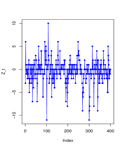
(a) Sample path of $\boldsymbol{\omega}_{1}$ .

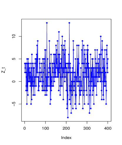
(b) Sample path of $\boldsymbol{\omega}_{2}$.

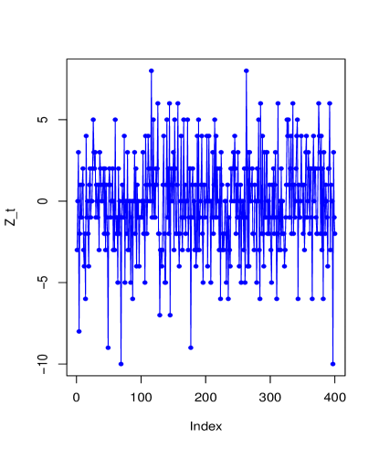
(c) Sample path of $\boldsymbol{\omega}_{3}$.

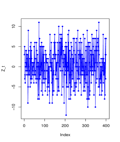
(d) Sample path of $\boldsymbol{\omega}_{4}$.

Figure 1: Sample paths of the four parameter groups.

4.3 Some Numerical Results

4.3.1 Results for CML and Yule-Walker

The performance of the estimators is checked by a small Monte Carlo simulation using different sample sizes ($n$ = 200, 400, 4000). All the simulations in this study are performed under the $R$ software based on $N=100$ replications. Table 2 gives mean and MSE for the conditional maximum likelihood and Yule-Walker method. Based on the table, we find that the estimates are convergent to their values. Within each case, parameter $\phi$ takes small value 0.2, and large value 0.8, 0.9. Moreover, we choose the case $\theta_{1}=\theta_{2}$ and the case $\theta_{1}\not=\theta_{2}$. Since the value of $\delta$ can be $1$ or $-1$, we also consider the estimation of the negative correlation cases. Table 1 and Table 2 show that obtained estimaters are convergent to their values in all the cases. Also, increasing the sample size implies smaller MSE. Moreover, we can notice that Yule-Walker estimator gives larger MSE in almost every case. All of the above, we can conclude that in most cases, the CMLEs provide good performance which was expected with respect to all parameters.

Table 1: Descriptive statistics of daily new cases in Barbados with lag one difference.

Variable	no.	Mean	Variance	Minimum	Median	Maximum	Range
Barbados. cases	292	1.3527	5.6037	0	0	16	16
Barbados. difference	291	-0.0068	8.4879	-14	0	14	28

Table 2: Mean value and mean square error (MSE) are reported for $mymodel^{+}$ and $mymodel^{-}$ through CML and Yule-walker method for $(\phi,p,\beta,\theta_{1},\theta_{2})^{\top}$ and with $n=200,400$, $800$ and $4000$.

$N$	$\phi_{ml}$	$p_{ml}$	$\beta_{ml}$	$\theta_{1ml}$	$\theta_{2ml}$	$\phi_{yw}$	$\theta_{1yw}$	$\theta_{2yw}$	$\theta_{1yw}-\theta_{2yw}$
(i) True values $\boldsymbol{\omega}_{1}=(0.8,0.5,\sqrt{5},10,10)^{\top},\delta=1$
200	0.8004	0.5009	2.2356	10.5380	10.3026	0.7908	15.3333	15.3913	-0.0580
MSE	0.0019	0.0024	0.1454	9.7403	9.7399	0.0185	332.3275	325.2845	1.5563
400	0.7952	0.4998	2.2161	10.1775	10.1759	0.7936	19.0681	19.2959	-0.2278
MSE	0.0014	0.0010	0.0662	4.0363	4.2060	0.0104	4347.6635	4729.4396	9.3705
800	0.7962	0.5006	2.2319	10.0079	10.0324	0.7893	12.0170	12.0429	-0.0258
MSE	0.0004	0.0006	0.0306	2.2122	1.9988	0.0050	32.7616	33.0771	0.2485
4000	0.8002	0.4996	2.2441	10.0126	10.0012	0.7938	11.0958	11.0919	0.0039
MSE	0.0001	0.0001	0.0079	0.3718	0.3577	0.0013	6.2700	6.2717	0.0288
(ii) True values $\boldsymbol{\omega}_{2}=(0.2,0.4,2,9,7)^{\top},\delta=1$
200	0.2304	0.4192	1.9630	9.1064	7.0075	0.1872	9.2269	7.1646	2.0622
MSE	0.0063	0.0128	3.7185	0.9755	0.9086	0.0397	8.6072	6.1845	0.2958
400	0.2125	0.3956	1.7688	9.0346	7.0050	0.2091	8.9010	6.8413	2.0597
MSE	0.0026	0.0044	2.5326	0.5209	0.4666	0.0152	1.8819	1.3431	0.1247
800	0.2043	0.4060	1.4135	9.0057	6.9987	0.2061	8.7288	6.6983	2.0304
MSE	0.0011	0.0027	0.3711	0.2784	0.2365	0.0112	1.2221	0.9268	0.0535
4000	0.1995	0.3994	1.4436	9.0136	7.0057	0.2058	8.5688	6.5613	2.0075
MSE	0.0002	0.0004	0.0836	0.0700	0.0603	0.0020	0.3844	0.3418	0.0110
(iv) True values $\boldsymbol{\omega}_{3}=(0.2,0.4,\sqrt{5},5,5)^{\top},\delta=-1$
200	0.2354	0.4093	3.6901	5.2991	5.2297	0.1782	4.9700	5.0335	-0.0635
MSE	0.0196	0.0326	26.8456	2.0729	1.9893	0.0372	2.5206	2.6660	0.0768
400	0.2127	0.4028	2.7968	5.0779	5.0616	0.1893	4.9007	4.8959	0.0047
MSE	0.0091	0.0120	7.9427	0.3761	0.3408	0.0191	0.8230	0.8166	0.0405
800	0.2227	0.3805	2.8852	5.1111	5.0912	0.1979	4.8497	4.8575	-0.0078
MSE	0.0067	0.0058	4.9466	0.2222	0.2192	0.0078	0.3244	0.3160	0.0175
4000	0.2026	0.4002	2.3019	4.9971	5.0057	0.2021	4.8513	4.8653	-0.0140
MSE	0.0005	0.0009	0.2648	0.0254	0.0258	0.0020	0.0894	0.0881	0.0039
(v) True values $\boldsymbol{\omega}_{4}=(0.2,0.8,\sqrt{5},10,10)^{\top},\delta=-1$
200	0.2150	0.7982	2.7313	9.9927	10.0072	0.1984	9.8042	9.7416	0.0626
MSE	0.0047	0.0062	7.8927	1.5760	1.4650	0.0088	1.7339	1.8601	0.1320
400	0.2067	0.7956	2.7468	9.9741	9.9550	0.2014	9.8563	9.8964	-0.0400
MSE	0.0012	0.0027	3.0378	0.5707	0.6029	0.0045	0.9554	0.9539	0.0788
800	0.2028	0.8006	2.3352	9.9443	9.9523	0.2010	9,8914	9.8812	0.0103
MSE	0.0008	0.0011	0.7012	0.3170	0.3108	0.0024	0.4759	0.4933	0.0391
4000	0.2018	0.8007	2.3115	10.0136	10.0214	0.2007	9.8885	9.8877	0.0008
MSE	0.0001	0.0002	0.1202	0.0654	0.0629	0.0005	0.1108	0.1094	0.0098

5 Real Data Example

Table 3: Estimated parameters through several models, AIC, BIC for the new cases in barbodos from to

Model	CML estimates	AIC	BIC	HQIC	Log-likelihood
$\text{PDINAR}^{-}(1)$	$\hat{\alpha}=-0.4187$	1365.8327	1376.8629	1365.0418	-679.9163
	$\hat{\theta}_{1}=1.7735$
	$\hat{\theta}_{2}=1.8309$
$\text{MESINAR}^{-}(1)$	$\hat{\phi}=0.5680$	1042.2406	1060.6243	1040.9225	-516.1203
	$\hat{p}=-0.0055$
	$\hat{\beta}=17.1567$
	$\hat{\theta}_{1}=3.8991$
	$\hat{\theta}_{2}=1.0149$
$\text{MSINARS}^{-}(1)$	$\hat{\phi}=0.4752$	1229.3335	1244.0405	1228.2790	-610.6668
	$\hat{\alpha}=-0.6932$
	$\hat{\theta}_{1}=5.3686$
	$\hat{\theta}_{2}=4.7866$

In this section,we apply our model to a real count data obtained from the website [1]. The series is about daily new cases in Barbados. We aim to study the change of incrememental of the data. The series represents the daily new cases of in Barbados from March, 17th 2020 to January, 2nd 2021.

The sample paths, the difference of the sample paths, autocorrelation functions (ACFs) and partial autocorrelation functions (PACFs) of two series are displayed in Figure 2. The figures suggest that the first order autoregressice models are appropriate for analysing the given data series.

Some series after differencing include negative values thus, the advantage of the model we proposed is to fit integer valued time series with possible negative values and either positive or negative correlation.

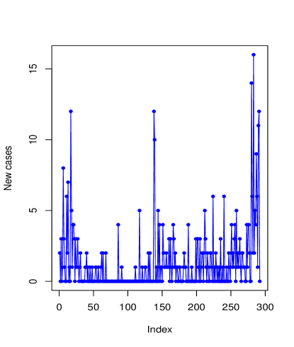
(a) Sample path of daily new cases.

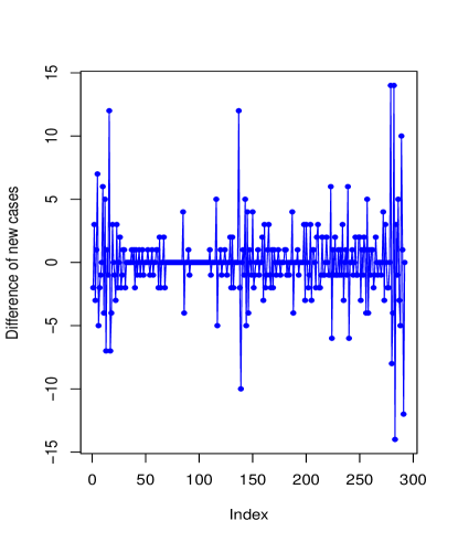
(b) Sample path of differenced daily new cases.

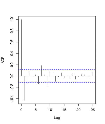
(c) ACF of differenced daily new cases.

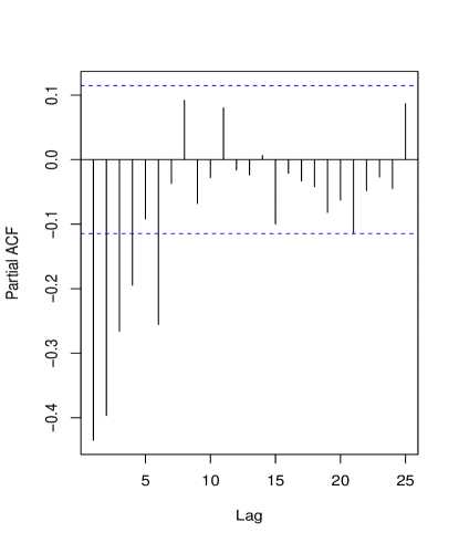
(d) PACF of differenced daily new cases.

Figure 2: Sample paths, ACF and PACF of differenced daily new cases.

The results are given in Table 1 and 3. Table 1 shows descriptive statistics of differenced daily new cases in Barbados with their lag one difference. According to the ACF of differenced daily new cases, the autocorrelation is negative, i.e., $\hat{\delta}=-1$. For the purpose of testing our model compared with other simple distributions or INAR(1) models, which can analyse positive and negative data, we apply some goodness-of-fit statistics criteria: AIC, BIC, HQIC and log-likelihood. For the purpose of testing our model against some other relevant INAR(1) models, such as $\text{PDINAR}(1)$ and the process $Z_{t}=U_{t}\left(\alpha\odot Z_{t-1}\right)+(1-U_{t})\varepsilon_{t}$, where $U_{t}$ is a sequence of independent and identically Bernoulli random variables with parameter $\phi$, $"\odot"$ is the operator proposed by Hee-young and Yousung[23], and $\left\{\varepsilon_{t}\right\}$ is a sequence of independent and identically Poisson difference distributed random variables with parameters $\theta_{1},\theta_{2}$.

Table 3 presents some goodness-of-fit statistics for the series. Better model is characterized by smaller values of these statistics. As it can be seen from these tables, the five statistics are small for the model we proposed. And the difference $\hat{\theta}_{1}-\hat{\theta}_{2}=2.8842$ shows that the innovation of original series is possibly not a single unchanged Poisson distribution. Therefore, we can conclude that the model works well for the real data series.

6 Conclusion and Prospect

In this paper, we construct a model based on extended binomial distribution and Skellam distribution with the Pegram’s operator dealing with positive or negative autocorrelation data defined on $\mathbf{Z}$. The best method of all is CML method via numerical simulation and it performs well on the number of differenced daily new cases in Barbados.

Next we will extend our model naturally to a SINARS regression model:

$$Z_{t} =(\phi,\delta S_{\alpha,\theta}(Z_{t-1}))*(1-\phi,R_{t}),t=1,2,\ldots$$

$$R_{t} \sim\operatorname{Skellam}\left(\theta_{1t},\theta_{2}\right)$$

$$\theta_{1t} =\beta_{0}+\beta_{1}X_{1t}+\ldots+\beta_{k}X_{kt}$$

where $X_{it}$ are covariates and the $\beta$’s the associated coefficients.

Another extension is that we consider a mixture of Bivariate Skellam distribution [33] and Bivariate extended binomial distribution to deal with binary data.

Acknowledgments.  Our research was supported by Jilin University and Liaoning University.

Appendix A Appendix

A.1 Proof of theorem 1

The proof of the theorem follows Theorem 2.1 of Billingsley[9]. We show the conditions(C1)-(C6) are satisfied for the model. We first give one lemma, which plays a key role in the proofs of other lemmas.

1. $P(m,n)$ is three times continuously differentiable with respect to $\phi,p,\theta,\theta_{1},\theta_{2}$, and for any $m$,$\{n;P(m,n)>0\}$ does not depend on $\omega$. Therefore, $\log P(m,n)$ is well-defined except on a set of $P(m,\cdot)$-measure 0 which does not depend on the parameter values. Thus, conditions (C1) and (C2) are satisfied for the model.

2. Recall the one step transition probability is

   $$\pi(z_{t}|z_{t-1}) =P(Z_{t}=z_{t}|Z_{t-1}=z_{t-1})$$

   $$=\phi P(S_{\alpha,\theta}(Z_{t-1})=\delta z_{t})+(1-\phi)P(\varepsilon_{t}=z_{t})$$

   $$=\phi\frac{I_{\delta z_{t}}(2p\beta)I_{z_{t-1}-\delta z_{t}}(2(1-p)\beta)}{I_{z_{t-1}}(2\beta)}+(1-\phi)e^{-\theta_{1}-\theta_{2}}\left(\frac{\theta_{1}}{\theta_{2}}\right)^{z_{t}/2}I_{z_{t}}\left(2\sqrt{\theta_{1}\theta_{2}}\right)$$

   Using the derivative formula of modified Bessel function of the first kind:

   $$\frac{\partial I_{y}(\theta)}{\partial\theta}=\frac{y}{\theta}I_{y}(\theta)+I_{y+1}(\theta).$$

   Without loss of generality, and in order to simplify the problem, we consider the case $\delta=1$ (The case $\delta=-1$ is similarly obtained).
   Let $P(m,n)=P(Z_{t}=n|Z_{t-1}=m)=\phi Z(m,n)+(1-\phi)q(m,n)$,
   where

   $$Z(m,n)=\frac{I_{n}(2p\beta)I_{m-n}(2(1-p)\beta)}{I_{m}(2\beta)},$$

   and

   $$q(m,n)=e^{-\theta_{1}-\theta_{2}}\left(\frac{\theta_{1}}{\theta_{2}}\right)^{n/2}I_{n}\left(2\sqrt{\theta_{1}\theta_{2}}\right).$$

   Thus

   $$P(m,n)\leq Z(m,n)+q(m,n).$$

   And for the first order derivative of transition probability, we have

   $$\sum_{n=-\infty}^{\infty}\left|\frac{\partial P(m,n)}{\partial\phi}\right|=\sum_{n=-\infty}^{\infty}\left|Z(m,n)-q(m,n)\right|\leq\sum_{n=-\infty}^{\infty}\left|Z(m,n)\right|+\sum_{n=-\infty}^{\infty}\left|q(m,n)\right|=2<\infty,$$

   the second derivative with respect to $\phi$ is equal to zero. And the derivative can be simplied as follows:

   $$\left|\frac{\partial P(m,n)}{\partial p}\right|=\left|\frac{\partial Z(m,n)}{\partial p}\right|,\left|\frac{\partial P(m,n)}{\partial\beta}\right|=\left|\frac{\partial Z(m,n)}{\partial\beta}\right|,$$

   $$\left|\frac{\partial P(m,n)}{\partial\theta_{1}}\right|=\left|\frac{\partial q(m,n)}{\partial\theta_{1}}\right|,\left|\frac{\partial P(m,n)}{\partial\theta_{2}}\right|=\left|\frac{\partial q(m,n)}{\partial\theta_{2}}\right|.$$

   Further we have

   $$\frac{\partial Z(m,n)}{\partial p} =-\frac{\beta\phi I_{n}(2p\beta)(I_{m-n-1}(2(1-p)\beta)+I_{m-n+1}(2(1-p)\beta))}{I_{m}(2\beta)}$$

   $$\quad+\frac{\beta\phi(I_{n-1}(2p\beta)+I_{n+1}(2p\beta))I_{m-n}(2(1-p)\beta)}{I_{m}(2\beta)},$$

   $$\frac{\partial Z(m,n)}{\partial\beta} =-\frac{\phi(I_{m-1}(2\beta)+I_{m+1}(2\beta))I_{n}(2p\beta)I_{m-n}(2(1-p)\beta)}{I_{m}(2\beta){}^{2}}$$

   $$\quad+(1-p)\phi\frac{I_{n}(2p\beta)(I_{m-n-1}(2(1-p)\beta)+I_{m-n+1}(2(1-p)\beta))}{I_{m}(2\beta)}$$

   $$\quad+\frac{p\phi(I_{n-1}(2p\beta)+I_{n+1}(2p\beta))I_{m-n}(2(1-p)\beta)}{I_{m}(2\beta)},$$

   $$\frac{\partial^{2}Z(m,n)}{\partial p^{2}} =\phi(-\beta I_{n}(2p\beta)(-\beta(I_{m-n-2}(2(1-p)\beta)+I_{m-n}(2(1-p)\beta))$$

   $$\quad-\beta(I_{m-n}(2(1-p)\beta)+I_{m-n+2}(2(1-p)\beta)))$$

   $$\quad-2\beta^{2}(I_{n-1}(2p\beta)+I_{n+1}(2p\beta))(I_{m-n-1}(2(1-p)\beta)+I_{m-n+1}(2(1-p)\beta))$$

   $$\quad+\beta(\beta(I_{n-2}(2p\beta)+I_{n}(2p\beta))+\beta(I_{n}(2p\beta)+I_{n+2}(2p\beta)))I_{m-n}(2(1-p)\beta)),$$

   $$\frac{\partial^{2}Z(m,n)}{\partial\beta^{2}} =\phi\left(\frac{2(I_{m-1}(2\beta)+I_{m+1}(2\beta)){}^{2}}{I_{m}(2\beta){}^{3}}-\frac{I_{m-2}(2\beta)+2I_{m}(2\beta)+I_{m+2}(2\beta)}{I_{m}(2\beta){}^{2}}\right)$$

   $$\quad\cdot I_{n}(2p\beta)I_{m-n}(2(1-p)\beta)-\frac{2\phi(I_{m-1}(2\beta)+I_{m+1}(2\beta))}{I_{m}(2\beta){}^{2}}$$

   $$\quad\cdot(1-p)I_{n}(2p\beta)(I_{m-n-1}(2(1-p)\beta)+I_{m-n+1}(2(1-p)\beta))$$

   $$\quad+p(I_{n-1}(2p\beta)+I_{n+1}(2p\beta))I_{m-n}(2(1-p)\beta)$$

   $$\quad(1-p)((1-p)(I_{m-n-2}(2(1-p)\beta)+I_{m-n}(2(1-p)\beta))$$

   $$\quad+(1-p)(I_{m-n}(2(1-p)\beta)+I_{m-n+2}(2(1-p)\beta))),$$

   $$\frac{\partial^{2}Z(m,n)}{\partial p\partial\beta} =-\frac{\phi I_{n}(2p\beta)(I_{m-n-1}(2(1-p)\beta)+I_{m-n+1}(2(1-p)\beta))}{I_{m}(2\beta)}$$

   $$\quad+\frac{\beta\phi(I_{m-1}(2\beta)+I_{m+1}(2\beta))I_{n}(2p\beta)(I_{m-n-1}(2(1-p)\beta)+I_{m-n+1}(2(1-p)\beta))}{I_{m}(2\beta){}^{2}}$$

   $$\quad-\frac{\beta\phi I_{n}(2p\beta)((1-p)(I_{m-n-2}(2(1-p)\beta)+I_{m-n}(2(1-p)\beta))}{I_{m}(2\beta)}$$

   $$\quad+\frac{(1-p)(I_{m-n}(2(1-p)\beta)+I_{m-n+2}(2(1-p)\beta)))}{I_{m}(2\beta)}$$

   $$\quad+\frac{\phi(I_{n-1}(2p\beta)+I_{n+1}(2p\beta))I_{m-n}(2(1-p)\beta)}{I_{m}(2\beta)}$$

   $$\quad-\frac{\beta\phi(I_{m-1}(2\beta)+I_{m+1}(2\beta))(I_{n-1}(2p\beta)+I_{n+1}(2p\beta))I_{m-n}(2(1-p)\beta)}{I_{m}(2\beta){}^{2}}$$

   $$\quad+\frac{\beta(1-p)\phi(I_{n-1}(2p\beta)+I_{n+1}(2p\beta))(I_{m-n-1}(2(1-p)\beta)+I_{m-n+1}(2(1-p)\beta))}{I_{m}(2\beta)}$$

   $$\quad-\frac{\beta p\phi(I_{n-1}(2p\beta)+I_{n+1}(2p\beta))(I_{m-n-1}(2(1-p)\beta)+I_{m-n+1}(2(1-p)\beta))}{I_{m}(2\beta)}$$

   $$\quad+\frac{\beta\phi(p(I_{n-2}(2p\beta)+I_{n}(2p\beta))+p(I_{n}(2p\beta)+I_{n+2}(2p\beta)))I_{m-n}(2(1-p)\beta)}{I_{m}(2\beta)}.$$

   Based on the properties of the modified Bessel function of the first kind,

   $$\sum_{y=-\infty}^{\infty}\left(\frac{\theta_{1}}{\theta_{2}}\right)^{\frac{y}{2}}I_{y}\left(2\sqrt{\theta_{1}\theta_{2}}\right)=e^{\theta_{1}+\theta_{2}},$$

   $$\sum_{y=-\infty}^{\infty}y\left(\frac{\theta_{1}}{\theta_{2}}\right)^{\frac{y}{2}}I_{y}\left(2\sqrt{\theta_{1}\theta_{2}}\right)=\left(\theta_{1}-\theta_{2}\right)e^{\theta_{1}+\theta_{2}},$$

   $$\sum_{y=-\infty}^{\infty}y^{2}\left(\frac{\theta_{1}}{\theta_{2}}\right)^{\frac{y}{2}}I_{y}\left(2\sqrt{\theta_{1}\theta_{2}}\right)=\left(\theta_{1}+\theta_{2}+\left(\theta_{1}-\theta_{2}\right)^{2}\right)e^{\theta_{1}+\theta_{2}},$$

   $$I_{y}(\theta)=I_{-y}(\theta),\sum_{y=-\infty}^{\infty}I_{y}(\theta)=e^{\theta},\sum_{y=-\infty}^{\infty}yI_{y}(\theta)=0,$$

   $$\sum_{y=-\infty}^{\infty}y^{2}I_{y}(\theta)=\theta e^{\theta}\quad\forall\theta>0,\frac{\partial I_{y}(\theta)}{\partial\theta}=\frac{1}{2}\left(I_{y-1}(\theta)+I_{y+1}(\theta)\right),$$

   thus,

   $$\frac{e^{\theta}}{2}\leq\sum_{y=0}^{\infty}yI_{y}(\theta)\leq\frac{\theta e^{\theta}}{2},$$

   and

   $$e^{\theta}\leq 2\sum_{y=0}^{\infty}yI_{y}(\theta)=2\sum_{y=0}^{\infty}\left|yI_{y}(\theta)\right|\leq 2\sum_{y=0}^{\infty}y^{2}\left|I_{y}(\theta)\right|\leq\theta e^{\theta},$$

   Then, for $\frac{\partial Z(m,n)}{\partial p}$, The problem is to estimate the bound of

   $$\sum_{y=-\infty}^{\infty}\frac{I_{y}(2p\beta)I_{m-y-1}(2(1-p)\beta)}{I_{m}(2\beta)},$$

   it is obvious that

   $$\sum_{y=-\infty}^{\infty}\frac{I_{y}(2p\beta)I_{m-y-1}(2(1-p)\beta)}{I_{m}(2\beta)}=\frac{1}{I_{m}(2\beta)}\sum_{y=-\infty}^{\infty}I_{y}(2p\beta)I_{m-y-1}(2(1-p)\beta),$$

   thus we only need to bound

   $$\sum_{y=-\infty}^{\infty}I_{y}(2p\beta)I_{m-y-1}(2(1-p)\beta),$$

   by symmestry,

   $$\sum_{y=-\infty}^{\infty}I_{y}(2p\beta)I_{m-y-1}(2(1-p)\beta)=\sum_{y=-\infty}^{\infty}I_{y}(2p\beta)I_{y-m+1}(2(1-p)\beta).$$

   Now we consider the value of $I_{y}(\theta)$. We know that for fixed $\theta$,

   $$\sum_{y=0}^{\infty}I_{y}(\theta)=\frac{e^{\theta}}{2},$$

   and there is a constant $M$ such that

   $$\frac{e^{\theta}}{2}\leq M,$$

   thus the number of $y$ such that $|I_{y}(\theta)|\leq 1$ is almost $M-1$. Thus other infinitely many $y$ satisfy $|I_{y}(\theta)|<1$, moreover, $I_{y}(\theta)^{2}\leq|I_{y}(\theta)|$. Denote $I=\sum_{y=-\infty}^{\infty}I_{y}(2p\beta)I_{y-m+1}(2(1-p)\beta).$ We can find large enough constant $M$ such that

   $$I =\sum_{y=k_{1}}^{k_{M}}I_{y}(2p\beta)I_{y-m+1}(2(1-p)\beta)+\sum_{y=k_{M+1}}^{\infty}I_{y}(2p\beta)I_{y-m+1}(2(1-p)\beta)$$

   $$\leq\sum_{y=k_{1}}^{k_{M}}I_{y}(2p\beta)I_{y-m+1}(2(1-p)\beta)+\frac{1}{2}\sum_{y=k_{M+1}}^{\infty}\left(I_{y}(2p\beta)^{2}+I_{y-m+1}(2(1-p)\beta)^{2}\right)$$

   $$\leq\sum_{y=k_{1}}^{k_{M}}I_{y}(2p\beta)I_{y-m+1}(2(1-p)\beta)+\frac{1}{2}\sum_{y=k_{M+1}}^{\infty}\left(I_{y}(2p\beta)+I_{y-m+1}(2(1-p)\beta)\right)$$

   where $k_{1},k_{2},\ldots,k_{M},k_{M+1},\ldots$ is a rearrangement of $N$ such that when $y\in\{k_{1},k_{2},\ldots,k_{M}\}$, $|I_{y}(\theta)|\geq 1$, and when $y\in\{k_{M},\ldots,\}$, $|I_{y}(\theta)|<1$. It can be seen that the former of the right of the inequation is finite, and the latter is convergent. For higher derivatives, the problem to deal with is the product of more Bessel functions, and the rest follows the same pattern. Thus, we can see that, for fixed $m$,

   $$\sum_{n=-\infty}^{\infty}\left|\frac{\partial Z(m,n)}{\partial p}\right|<\infty,\sum_{n=-\infty}^{\infty}\left|\frac{\partial Z(m,n)}{\partial\beta}\right|<\infty,$$

   $$\sum_{n=-\infty}^{\infty}\left|\frac{\partial^{2}Z(m,n)}{\partial p^{2}}\right|<\infty,\sum_{n=-\infty}^{\infty}\left|\frac{\partial^{2}Z(m,n)}{\partial\beta^{2}}\right|<\infty,\sum_{n=-\infty}^{\infty}\left|\frac{\partial^{2}Z(m,n)}{\partial p\partial\beta}\right|<\infty.$$

   Next we are on the position to discuss the derivative of $q(m,n)$.

   $$\frac{\partial q(m,n)}{\partial\theta_{1}} =-e^{-\theta_{1}-\theta_{2}}\left(\frac{\theta_{1}}{\theta_{2}}\right)^{n/2}I_{n}\left(2\sqrt{\theta_{1}\theta_{2}}\right)$$

   $$\quad+\frac{1}{2\theta_{2}}ne^{-\theta_{1}-\theta_{2}}\left(\frac{\theta_{1}}{\theta_{2}}\right)^{\frac{n}{2}-1}I_{n}\left(2\sqrt{\theta_{1}\theta_{2}}\right)$$

   $$\quad+\frac{1}{2\sqrt{\theta_{1}\theta_{2}}}\theta_{2}e^{-\theta_{1}-\theta_{2}}\left(\frac{\theta_{1}}{\theta_{2}}\right)^{n/2}\left(I_{n-1}\left(2\sqrt{\theta_{1}\theta_{2}}\right)+I_{n+1}\left(2\sqrt{\theta_{1}\theta_{2}}\right)\right),$$

   $$\frac{\partial q(m,n)}{\partial\theta_{2}} =-e^{-\theta_{1}-\theta_{2}}\left(\frac{\theta_{1}}{\theta_{2}}\right)^{n/2}I_{n}\left(2\sqrt{\theta_{1}\theta_{2}}\right)$$

   $$\quad-\frac{1}{2\theta_{2}^{2}}\theta_{1}ne^{-\theta_{1}-\theta_{2}}\left(\frac{\theta_{1}}{\theta_{2}}\right)^{\frac{n}{2}-1}I_{n}\left(2\sqrt{\theta_{1}\theta_{2}}\right)$$

   $$\quad+\frac{1}{2\sqrt{\theta_{1}\theta_{2}}}\theta_{1}e^{-\theta_{1}-\theta_{2}}\left(\frac{\theta_{1}}{\theta_{2}}\right)^{n/2}\left(I_{n-1}\left(2\sqrt{\theta_{1}\theta_{2}}\right)+I_{n+1}\left(2\sqrt{\theta_{1}\theta_{2}}\right)\right),$$

   $$\frac{\partial^{2}q(m,n)}{\partial\theta^{2}_{1}} =\left(\frac{\left(\frac{n}{2}-1\right)ne^{-\theta_{1}-\theta_{2}}\left(\frac{\theta_{1}}{\theta_{2}}\right)^{\frac{n}{2}-2}}{2\theta_{2}^{2}}+e^{-\theta_{1}-\theta_{2}}\left(\frac{\theta_{1}}{\theta_{2}}\right)^{n/2}-\frac{ne^{-\theta_{1}-\theta_{2}}\left(\frac{\theta_{1}}{\theta_{2}}\right)^{\frac{n}{2}-1}}{\theta_{2}}\right)I_{n}\left(2\sqrt{\theta_{1}\theta_{2}}\right)$$

   $$\quad+\left(\frac{ne^{-\theta_{1}-\theta_{2}}\left(\frac{\theta_{1}}{\theta_{2}}\right)^{\frac{n}{2}-1}}{2\theta_{2}}-e^{-\theta_{1}-\theta_{2}}\left(\frac{\theta_{1}}{\theta_{2}}\right)^{n/2}\right)\left(I_{n-1}\left(2\sqrt{\theta_{1}\theta_{2}}\right)+I_{n+1}\left(2\sqrt{\theta_{1}\theta_{2}}\right)\right)\frac{\theta_{2}}{\sqrt{\theta_{1}\theta_{2}}}$$

   $$\quad+\left(I_{n-2}\left(2\sqrt{\theta_{1}\theta_{2}}\right)+2I_{n}\left(2\sqrt{\theta_{1}\theta_{2}}\right)+I_{n+2}\left(2\sqrt{\theta_{1}\theta_{2}}\right)\right)e^{-\theta_{1}-\theta_{2}}\left(\frac{\theta_{1}}{\theta_{2}}\right)^{n/2}\frac{\theta_{2}}{4\theta_{1}}$$

   $$\quad-\left(I_{n-1}\left(2\sqrt{\theta_{1}\theta_{2}}\right)+I_{n+1}\left(2\sqrt{\theta_{1}\theta_{2}}\right)\right)e^{-\theta_{1}-\theta_{2}}\left(\frac{\theta_{1}}{\theta_{2}}\right)^{n/2}\frac{\theta_{2}^{2}}{4(\theta_{1}\theta_{2})^{3/2}},$$

   $$\frac{\partial^{2}q(m,n)}{\partial\theta^{2}_{2}} =\left(\frac{\theta_{1}^{2}\left(\frac{n}{2}-1\right)n\left(\frac{\theta_{1}}{\theta_{2}}\right)^{\frac{n}{2}-2}}{2\theta_{2}^{4}}+\frac{\theta_{1}n\left(\frac{\theta_{1}}{\theta_{2}}\right)^{\frac{n}{2}-1}}{\theta_{2}^{3}}\right)I_{n}\left(2\sqrt{\theta_{1}\theta_{2}}\right)e^{-\theta_{1}-\theta_{2}}$$

   $$\quad+\left(\frac{\theta_{1}ne^{-\theta_{1}-\theta_{2}}\left(\frac{\theta_{1}}{\theta_{2}}\right)^{\frac{n}{2}-1}}{\theta_{2}^{2}}+e^{-\theta_{1}-\theta_{2}}\left(\frac{\theta_{1}}{\theta_{2}}\right)^{n/2}\right)I_{n}\left(2\sqrt{\theta_{1}\theta_{2}}\right)$$

   $$\quad+\left(-\frac{\theta_{1}ne^{-\theta_{1}-\theta_{2}}\left(\frac{\theta_{1}}{\theta_{2}}\right)^{\frac{n}{2}-1}}{2\theta_{2}^{2}}-e^{-\theta_{1}-\theta_{2}}\left(\frac{\theta_{1}}{\theta_{2}}\right)^{n/2}\right)\frac{\theta_{1}}{\sqrt{\theta_{1}\theta_{2}}}$$

   $$\quad\quad\cdot\left(I_{n-1}\left(2\sqrt{\theta_{1}\theta_{2}}\right)+I_{n+1}\left(2\sqrt{\theta_{1}\theta_{2}}\right)\right)$$

   $$\quad-\left(I_{n-1}\left(2\sqrt{\theta_{1}\theta_{2}}\right)+I_{n+1}\left(2\sqrt{\theta_{1}\theta_{2}}\right)\right)e^{-\theta_{1}-\theta_{2}}\left(\frac{\theta_{1}}{\theta_{2}}\right)^{n/2}\frac{\theta_{1}^{2}}{4(\theta_{1}\theta_{2})^{3/2}}$$

   $$\quad+\left(I_{n-2}\left(2\sqrt{\theta_{1}\theta_{2}}\right)+2I_{n}\left(2\sqrt{\theta_{1}\theta_{2}}\right)+I_{n+2}\left(2\sqrt{\theta_{1}\theta_{2}}\right)\right)e^{-\theta_{1}-\theta_{2}}\left(\frac{\theta_{1}}{\theta_{2}}\right)^{n/2}\frac{\theta_{1}^{2}}{4\theta_{1}\theta_{2}},$$

   $$\frac{\partial^{2}q(m,n)}{\partial\theta_{1}\partial\theta_{2}} =-\frac{1}{2\theta_{2}}ne^{-\theta_{1}-\theta_{2}}\left(\frac{\theta_{1}}{\theta_{2}}\right)^{\frac{n}{2}-1}I_{n}\left(2\sqrt{\theta_{1}\theta_{2}}\right)+e^{-\theta_{1}-\theta_{2}}\left(\frac{\theta_{1}}{\theta_{2}}\right)^{n/2}I_{n}\left(2\sqrt{\theta_{1}\theta_{2}}\right)$$

   $$\quad-\left(\frac{n}{2}-1\right)ne^{-\theta_{1}-\theta_{2}}\left(\frac{\theta_{1}}{\theta_{2}}\right)^{\frac{n}{2}-2}\frac{\theta_{1}}{2\theta_{2}^{3}}I_{n}\left(2\sqrt{\theta_{1}\theta_{2}}\right)$$

   $$\quad+\frac{(\theta_{1}-1)}{2\theta_{2}^{2}}ne^{-\theta_{1}-\theta_{2}}\left(\frac{\theta_{1}}{\theta_{2}}\right)^{\frac{n}{2}-1}I_{n}\left(2\sqrt{\theta_{1}\theta_{2}}\right)$$

   $$\quad-\frac{\theta_{1}\theta_{2}}{4(\theta_{1}\theta_{2})^{3/2}}e^{-\theta_{1}-\theta_{2}}\left(\frac{\theta_{1}}{\theta_{2}}\right)^{n/2}\left(I_{n-1}\left(2\sqrt{\theta_{1}\theta_{2}}\right)+I_{n+1}\left(2\sqrt{\theta_{1}\theta_{2}}\right)\right)$$

   $$\quad+\frac{(1-\theta_{1}-\theta_{2})}{2\sqrt{\theta_{1}\theta_{2}}}e^{-\theta_{1}-\theta_{2}}\left(\frac{\theta_{1}}{\theta_{2}}\right)^{n/2}\left(I_{n-1}\left(2\sqrt{\theta_{1}\theta_{2}}\right)+I_{n+1}\left(2\sqrt{\theta_{1}\theta_{2}}\right)\right)$$

   $$\quad+\frac{1}{4}\left(I_{n-2}\left(2\sqrt{\theta_{1}\theta_{2}}\right)+2I_{n}\left(2\sqrt{\theta_{1}\theta_{2}}\right)+I_{n+2}\left(2\sqrt{\theta_{1}\theta_{2}}\right)\right)e^{-\theta_{1}-\theta_{2}}\left(\frac{\theta_{1}}{\theta_{2}}\right)^{n/2}.$$

   And we rewrite the derivatives as follows:

   $$\frac{\partial q(m,n)}{\partial\theta_{1}}=\left(\frac{n}{2\theta_{1}}-1\right)q(m,n)+\frac{1}{2}q(m,n-1)+\frac{\theta_{2}}{2\theta_{1}}q(m,n+1),$$

   $$\frac{\partial q(m,n)}{\partial\theta_{2}}=\left(-\frac{n}{2\theta_{1}}-1\right)q(m,n)+\frac{\theta_{1}}{2\theta_{2}}q(m,n-1)+\frac{1}{2}q(m,n+1),$$

   $$\frac{\partial^{2}q(m,n)}{\partial\theta_{1}^{2}} =\left(\frac{n^{2}-2n}{4\theta_{1}^{2}}-\frac{n}{\theta_{1}}+1\right)q(m,n)+\left(\frac{2n-1}{4\theta_{1}}-1\right)q(m,n-1)$$

   $$\quad+\left(\frac{(2n-\theta_{1})\theta_{2}}{4\theta_{1}^{2}}-\frac{\theta_{2}}{\theta_{1}}\right)q(m,n+1)+\frac{1}{2}q(m,n-2),$$

   $$\frac{\partial^{2}q(m,n)}{\partial\theta_{2}^{2}} =\left(\frac{n^{2}-2n}{4\theta_{2}^{2}}+e^{-\theta_{1}-\theta_{2}}+\frac{2n}{\theta_{2}}\right)q(m,n)+\left(\frac{\theta_{1}}{4\theta_{2}^{2}}-1-\frac{n\theta_{1}^{2}}{2\theta_{2}^{3}}\right)q(m,n-1)$$

   $$\quad+\left(\frac{1}{4\theta_{2}}-1-\frac{n}{2\sqrt{\theta_{1}\theta_{2}}}\right)q(m,n+1)+\frac{\theta_{1}^{2}}{2\theta_{2}^{2}}q(m,n-2),$$

   since the modified Bessel function of the first kind is bounded, thus it is obvious that

   $$\left|\sum_{n=-\infty}^{\infty}\frac{\partial q(m,n)}{\partial\theta_{1}}\right|<\infty,\left|\sum_{n=-\infty}^{\infty}\frac{\partial q(m,n)}{\partial\theta_{2}}\right|<\infty,$$

   $$\left|\sum_{n=-\infty}^{\infty}\frac{\partial^{2}q(m,n)}{\partial\theta_{1}^{2}}\right|<\infty,\left|\sum_{n=-\infty}^{\infty}\frac{\partial^{2}q(m,n)}{\partial\theta_{1}^{2}}\right|<\infty.$$

   Furthermore, the series converges absolutely, and we obtain

   $$\sum_{n=-\infty}^{\infty}\left|\frac{\partial q(m,n)}{\partial\theta_{1}}\right|<\infty,\sum_{n=-\infty}^{\infty}\left|\frac{\partial q(m,n)}{\partial\theta_{2}}\right|<\infty,$$

   $$\sum_{n=-\infty}^{\infty}\left|\frac{\partial^{2}q(m,n)}{\partial\theta_{1}^{2}}\right|<\infty,\sum_{n=-\infty}^{\infty}\left|\frac{\partial^{2}q(m,n)}{\partial\theta_{1}^{2}}\right|<\infty.$$

   Consequently, the condition (C4) is satisfied.

   Now we caculate the log-partial derivatives for the unknown parameters as follows.
   For the first order derivatives, we have

   $$\begin{gathered}\left|\frac{\partial\log P(m,n)}{\partial\phi}\right|=\left|\frac{Z(m,n)-q(m,n)}{P(m,n)}\right|\leq\frac{Z(m,n)}{P(m,n)}+\frac{q(m,n)}{P(m,n)}\leq\frac{1}{\phi(1-\phi)},\end{gathered}$$

   $$\left|\frac{\partial\log P(m,n)}{\partial p}\right|=\left|\frac{1}{P(m,n)}\frac{\partial P(m,n)}{\partial p}\right|\leq\psi(m,n)\left|\frac{\partial P(m,n)}{\partial p}\right|,$$

   $$\left|\frac{\partial\log P(m,n)}{\partial\beta}\right|=\left|\frac{1}{P(m,n)}\frac{\partial P(m,n)}{\partial\beta}\right|\leq\psi(m,n)\left|\frac{\partial P(m,n)}{\partial\beta}\right|,$$

   $$\left|\frac{\partial\log P(m,n)}{\partial\theta_{1}}\right|=\left|\frac{1}{P(m,n)}\frac{\partial P(m,n)}{\partial\theta_{1}}\right|\leq\psi(m,n)\left|\frac{\partial P(m,n)}{\partial\theta_{1}}\right|,$$

   $$\left|\frac{\partial\log P(m,n)}{\partial\theta_{2}}\right|=\left|\frac{1}{P(m,n)}\frac{\partial P(m,n)}{\partial\theta_{2}}\right|\leq\psi(m,n)\left|\frac{\partial P(m,n)}{\partial\theta_{2}}\right|,$$

   where $\psi$ is a constant relevant to $m$ and $n$, and combined with the above results, the first derivatives can be bounded by some appropriate constant, respectively. We know that in the stationary state

   $$E\left|\frac{\partial\log P\left(Z_{1},Z_{2}\right)}{\partial\phi}\right|^{2}<\infty,E\left|\frac{\partial\log P\left(Z_{1},Z_{2}\right)}{\partial p}\right|^{2}<\infty,$$

   $$E\left|\frac{\partial\log P\left(Z_{1},Z_{2}\right)}{\partial\beta}\right|^{2}<\infty,E\left|\frac{\partial\log P\left(Z_{1},Z_{2}\right)}{\partial\theta_{1}}\right|^{2}<\infty,E\left|\frac{\partial\log P\left(Z_{1},Z_{2}\right)}{\partial\theta_{2}}\right|^{2}<\infty.$$

   Due to the length of the paper, we will not present the second and third order derivatives, the core problem of estimating the bound of derivatives is the method to estimate the bound of product of Bessel functions when $m$ is fixed.
   Analogously, denote $\boldsymbol{\omega}_{1}=\phi$, $\boldsymbol{\omega}_{2}=p$, $\boldsymbol{\omega}_{3}=\beta$, $\boldsymbol{\omega}_{4}=\theta_{1}$, $\boldsymbol{\omega}_{5}=\theta_{2}$,

   $$E\left|\frac{\partial^{2}\log P\left(Z_{1},Z_{2}\right)}{\partial\boldsymbol{\omega}_{u}\partial\boldsymbol{\omega}_{v}}\right|^{2}<\infty,E\left|\frac{\partial^{3}\log P\left(Z_{1},Z_{2}\right)}{\partial\boldsymbol{\omega}_{u}\partial\boldsymbol{\omega}_{v}\partial\boldsymbol{\omega}_{w}}\right|<\infty,\quad u,v,w=1,2,\ldots,5.$$

   The fisher information matrix $(\sigma_{ij})$ is well-defined and by (C6) it is nonsingular. We can conclude that the conditions (C1)-(C7) are satisfied. $\hfill\square$

   A.2 Proof of Existence of Stationary Solutions and Ergodic

   In this part we begin to show the existence of stationary solutions for the process $\{Z_{n}\}$, and prove that the stationary distribution is unique, then we present it is also aperiodic and ergodic. First we introduce the following proposition on the existence of stationary solutions for a Markov chain.

   Proposition A.2.1.

   If $\{Z_{n}\}$ is a weak Feller chain with state-space $Z$ and if for any $\eta>0$ there exists a compact set $C\subseteq Z$ such that $P(x,C^{c})<\eta$, for all $z\in Z$, where $P(x,C^{c})<\eta$ is the transition probability from $z$ to $C^{c}$, then $\{Z_{n}\}$ is bounded in probability and there exists at least one stationary distribution for the chain.

   Now we are on the position to verify whether the Markov chain satisfies Proposition A.2.1.

   Proof.

   We choose $C=\{-c,-c+1,\ldots,c-1,c\}$, where $c>0$ and $c\in\mathbb{N}$. It is obvious that $C$ is a compact set since the number of elements in $C$ is finite. By Markov’s inequality, we have

   $$\left\{\begin{aligned} &P(Z_{t}\geq c|Z_{t-1}=x)\leq\frac{E[Z_{t}|Z_{t-1}=x]}{c}=\frac{\phi p\delta x+(1-\phi)(\theta_{1}-\theta_{2})}{c},Z_{t}\geq 0,\\ &P(Z_{t}\leq-c|Z_{t-1}=x)\leq-\frac{E[Z_{t}|Z_{t-1}=x]}{c}=-\frac{\phi p\delta x+(1-\phi)(\theta_{1}-\theta_{2})}{c},Z_{t}<0.\\ \end{aligned}\right.$$

   Then, given $\eta>0$, choose enough large $c$ such that $\phi p\delta x+(1-\phi)(\theta_{1}-\theta_{2})<c\eta$. ∎

   We next turn to prove the uniqueness of a stationary distribution. We shall present $\{Z_{n}\}$ satisfies Doeblin’s condition, i.e., there exists a probability measure $\nu$ with the property that, for some $m\geq 1$, $\eta>0$, and $\gamma>0$, such that

   $$\nu(B)>\eta\Rightarrow P^{m}(x,B)\geq\gamma,\quad{\forall}x\in X.$$

   Then $\{Z_{n}\}$ has a unique stationary distribution and is uniformly ergodic. We need to verify whether the above conditions hold for $\{Z_{n}\}$.

   Proof.

   Define the measure $\nu$ to have unit point mass at $\{c\}$, where $c\in\mathbb{N}$. We only need to consider Borel sets $B$ with $c\in B$, and it is revealed that we can choose proper $\eta$ such that $\nu(\{c\})=\nu(B)>\eta$. Since $P(\{c\})<P(B)$, we have

   $$P(Z_{t}\in B|Z_{t-1}=x) \geq P(Z_{t}=c|Z_{t-1}=x)$$

   $$=\phi\frac{I_{\delta c}(2p\beta)I_{x-\delta c}(2(1-p)\beta)}{I_{x}(2\beta)}+(1-\phi)e^{-\theta_{1}-\theta_{2}}\left(\frac{\theta_{1}}{\theta_{2}}\right)^{c/2}I_{c}\left(2\sqrt{\theta_{1}\theta_{2}}\right).$$

   Case 1: If $\phi=0$, we can choose $\gamma$ such that

   $$P(Z_{t}\in B|Z_{t-1}=x) \geq P(Z_{t}=c|Z_{t-1}=x)=e^{-\theta_{1}-\theta_{2}}\left(\frac{\theta_{1}}{\theta_{2}}\right)^{c/2}I_{c}\left(2\sqrt{\theta_{1}\theta_{2}}\right)=\gamma>0.$$

   Case 2: If $\phi=1$, we can choose $\gamma$ such that

   $$P(Z_{t}\in B|Z_{t-1}=x) \geq P(Z_{t}=c|Z_{t-1}=x)=\frac{I_{\delta c}(2p\beta)I_{x-\delta c}(2(1-p)\beta)}{I_{x}(2\beta)}=\gamma>0.$$

   Case 3: If $0<\phi<1$, we can choose $\gamma$ such that

   $$P(Z_{t}\in B|Z_{t-1}=x) \geq P(Z_{t}=c|Z_{t-1}=x)$$

   $$=\phi\frac{I_{\delta c}(2p\beta)I_{x-\delta c}(2(1-p)\beta)}{I_{x}(2\beta)}+(1-\phi)e^{-\theta_{1}-\theta_{2}}\left(\frac{\theta_{1}}{\theta_{2}}\right)^{c/2}I_{c}\left(2\sqrt{\theta_{1}\theta_{2}}\right).$$

   $$=\gamma>0.$$

   Thus we can choose $m=1$, and Doeblin’s condition is satisfied. Denote $P(Z_{t}=x|Z_{t-1}=x)=P_{xx}$, for and we can calculate

   $$P_{xx}=\left\{\begin{aligned} &\phi\frac{I_{x}(2p\beta)I_{0}(2(1-p)\beta)}{I_{x}(2\beta)}+(1-\phi)e^{-\theta_{1}-\theta_{2}}\left(\frac{\theta_{1}}{\theta_{2}}\right)^{x/2}I_{x}\left(2\sqrt{\theta_{1}\theta_{2}}\right)>0,\delta=1,\\ &\phi\frac{I_{x}(2p\beta)I_{2x}(2(1-p)\beta)}{I_{x}(2\beta)}+(1-\phi)e^{-\theta_{1}-\theta_{2}}\left(\frac{\theta_{1}}{\theta_{2}}\right)^{x/2}I_{x}\left(2\sqrt{\theta_{1}\theta_{2}}\right)>0,\delta=-1.\\ \end{aligned}\right.$$

   Therefore, $\{Z_{n}\}$ is aperiodic, and we can conclude that $\{Z_{n}\}$ is uniformly ergodic. ∎

References

• [1] https://ourworldindata.org/covid-cases.
• [2] Mohamed A Al-Osh and Aus A Alzaid. First-order integer-valued autoregressive (INAR (1)) process. Journal of Time Series Analysis, 8(3):261–275, 1987.
• [3] A Alzaid and M Al-Osh. First-order integer-valued autoregressive (inar (1)) process: distributional and regression properties. Statistica Neerlandica, 42(1):53–61, 1988.
• [4] Abdulhamid A Alzaid and Mohamed A Al-Osh. Some autoregressive moving average processes with generalized Poisson marginal distributions. Annals of the Institute of Statistical Mathematics, 45:223–232, 1993.
• [5] Abdulhamid A Alzaid and Maha A Omair. On the Poisson difference distribution inference and applications. Bulletin of the Malaysian Mathematical Sciences Society. Second Series, 33(1):17–45, 2010.
• [6] Abdulhamid A Alzaid and Maha A Omair. An extended binomial distribution with applications. Communications in Statistics-Theory and Methods, 41(19):3511–3527, 2012.
• [7] Abdulhamid A Alzaid and Maha A Omair. Poisson difference integer valued autoregressive model of order one. Bulletin of the Malaysian Mathematical Sciences Society, 37(2):465–485, 2014.
• [8] Jonas Andersson and Dimitris Karlis. A parametric time series model with covariates for integers in Z. Statistical Modelling, 14(2):135–156, 2014.
• [9] Patrick Billingsley. Statistical methods in Markov chains. The annals of mathematical statistics, pages 12–40, 1961.
• [10] Patrick Billingsley. Convergence of probability measures. John Wiley & Sons, 2013.
• [11] Jan Bulla, Christophe Chesneau, and Maher Kachour. A bivariate first-order signed integer-valued autoregressive process. Communications in Statistics-Theory and Methods, 46(13):6590–6604, 2017.
• [12] Christophe Chesneau and Maher Kachour. A parametric study for the first-order signed integer-valued autoregressive process. Journal of Statistical Theory and Practice, 6:760–782, 2012.
• [13] Luc Devroye. Simulating Bessel random variables. Statistics & probability letters, 57(3):249–257, 2002.
• [14] J Franke and TH Seligmann. Conditional maximum likelihood estimates for INAR (1) processes and their application to modelling epileptic seizure counts. Developments in time series analysis, pages 310–330, 1993.
• [15] R Keith Freeland. True integer value time series. AStA Advances in Statistical Analysis, 94:217–229, 2010.
• [16] Arjun K Gupta and Saralees Nadarajah. Beta Bessel distributions. International journal of mathematics and mathematical sciences, 2006, 2006.
• [17] Peter Hall and Christopher C Heyde. Martingale limit theory and its application. Academic press, 2014.
• [18] Jie Huang and Fukang Zhu. A new first-order integer-valued autoregressive model with Bell innovations. Entropy, 23(6):713, 2021.
• [19] George Iliopoulos and Dimitris Karlis. Simulation from the Bessel distribution with applications. Journal of Statistical Computation and Simulation, 73(7):491–506, 2003.
• [20] SKELLAM JG. The frequency distribution of the difference between two Poisson variates belonging to different populations. Journal of the Royal Statistical Society. Series A (General), 109(Pt 3):296–296, 1946.
• [21] Maher Kachour and Lionel Truquet. A p-Order signed integer-valued autoregressive (SINAR (p)) model. Journal of Time Series Analysis, 32(3):223–236, 2011.
• [22] Dimitris Karlis and Ioannis Ntzoufras. Bayesian analysis of the differences of count data. Statistics in medicine, 25(11):1885–1905, 2006.
• [23] Hee-Young Kim and Yousung Park. A non-stationary integer-valued autoregressive model. Statistical papers, 49:485–502, 2008.
• [24] Lawrence A Klimko and Paul I Nelson. On conditional least squares estimation for stochastic processes. The Annals of statistics, pages 629–642, 1978.
• [25] AT McKay. A Bessel function distribution. Biometrika, pages 39–44, 1932.
• [26] Ed McKenzie. Some simple models for discrete variate time series 1. JAWRA Journal of the American Water Resources Association, 21(4):645–650, 1985.
• [27] Ed McKenzie. Autoregressive moving-average processes with negative-binomial and geometric marginal distributions. Advances in Applied probability, 18(3):679–705, 1986.
• [28] Ana V Miletić Ilić, Miroslav M Ristić, Aleksandar S Nastić, and Hassan S Bakouch. An INAR (1) model based on a mixed dependent and independent counting series. Journal of Statistical Computation and Simulation, 88(2):290–304, 2018.
• [29] Z Mohammadi, Z Sajjadnia, HS Bakouch, and M Sharafi. Zero-and-one inflated Poisson–Lindley INAR (1) process for modelling count time series with extra zeros and ones. Journal of Statistical Computation and Simulation, 92(10):2018–2040, 2022.
• [30] Zohreh Mohammadi, Zahra Sajjadnia, Maryam Sharafi, and Naushad Mamode Khan. Modeling Medical Data by Flexible Integer-Valued AR (1) Process with Zero-and-One-Inflated Geometric Innovations. Iranian Journal of Science and Technology, Transactions A: Science, 46(3):891–906, 2022.
• [31] Saralees Nadarajah and Arjun K Gupta. On the product and ratio of Bessel random variables. International Journal of Mathematics and Mathematical Sciences, 2005(18):2977–2989, 2005.
• [32] Aleksandar S Nastić, Miroslav M Ristić, and Ana V Miletić Ilić. A geometric time-series model with an alternative dependent Bernoulli counting series. Communications in Statistics-Theory and Methods, 46(2):770–785, 2017.
• [33] Maha A Omair, Ghadah A Alomani, and Abdulhamid A Alzaid. Bivariate Distributions on Z2. Bulletin of the Malaysian Mathematical Sciences Society, 45(Suppl 1):425–444, 2022.
• [34] GGS Pegram. An autoregressive model for multilag Markov chains. Journal of Applied Probability, 17(2):350–362, 1980.
• [35] Xiaohong Qi, Qi Li, and Fukang Zhu. Modeling time series of count with excess zeros and ones based on INAR (1) model with zero-and-one inflated poisson innovations. Journal of Computational and Applied Mathematics, 346:572–590, 2019.
• [36] Golnaz Shahtahmassebi and Rana Moyeed. An application of the generalized Poisson difference distribution to the Bayesian modelling of football scores. Statistica Neerlandica, 70(3):260–273, 2016.
• [37] Masoumeh Shirozhan and Mehrnaz Mohammadpour. An INAR (1) model based on the pegram and thinning operators with serially dependent innovation. Communications in Statistics-Simulation and Computation, 49(10):2617–2638, 2020.
• [38] Dag Tjøstheim. Estimation in nonlinear time series models. Stochastic Processes and their Applications, 21(2):251–273, 1986.
• [39] Dehui Wang and Haixiang Zhang. Generalized RCINAR (p) process with signed thinning operator. Communications in Statistics—Simulation and Computation®, 40(1):13–44, 2010.
• [40] Christian H Weiß. Thinning operations for modeling time series of counts—a survey. AStA Advances in Statistical Analysis, 92:319–341, 2008.
• [41] Kai Yang, Dehui Wang, Boting Jia, and Han Li. An integer-valued threshold autoregressive process based on negative binomial thinning. Statistical Papers, 59:1131–1160, 2018.
• [42] Lin Yuan and John D Kalbfleisch. On the Bessel distribution and related problems. Annals of the Institute of Statistical Mathematics, 52:438–447, 2000.
• [43] Scott L Zeger. A regression model for time series of counts. Biometrika, 75(4):621–629, 1988.
• [44] Chi Zhang, Guo-Liang Tian, and Kai-Wang Ng. Properties of the zero-and-one inflated Poisson distribution and likelihood-based inference methods. Statistics and its interface, 9(1):11–32, 2016.
• [45] Haixiang Zhang, Dehui Wang, and Fukang Zhu. Inference for INAR (p) processes with signed generalized power series thinning operator. Journal of Statistical Planning and Inference, 140(3):667–683, 2010.
• [46] Haitao Zheng, Ishwar V Basawa, and Somnath Datta. First-order random coefficient integer-valued autoregressive processes. Journal of Statistical Planning and Inference, 137(1):212–229, 2007.