Superoscillating Quantum Control Induced By Sequential Selections

Abstract

Superoscillation is a counterintuitive phenomenon for its mathematical feature of ”faster-than-Fourier”, which has allowed novel optical imaging beyond the diffraction limit. Here, we provide a superoscillating quantum control protocol realized by sequential selections in the framework of weak measurement, which drives the apparatus (target) by repeatedly applying optimal pre- and post-selections to the system (controller). Our protocol accelerates the adiabatic transport of trapped ions and adiabatic quantum search algorithm at a finite energy cost. We demonstrate the accuracy and robustness of the protocol in the presence of decoherence and fluctuating noise and elucidate the trade-off between fidelity and rounds of selections. Our findings provide avenues for quantum state control and wave-packet manipulation using superoscillation in quantum platforms such as trapped ions.

The concept of superoscillation (SO) was originally proposed as a footnote in a celebrated study on quantum measurement by Y. Aharonov et al. AAV in the late 1980s. The phenomenon occurs when a band-limited wave function varies arbitrarily faster than its fastest Fourier components, as allowed by its spectral content. In other words, a superoscillatory wave is a local feature that oscillates at a much higher frequency than the overall frequency of the global band-limited wave. This counterintuitive but physically allowed property is dubbed as faster-than-Fourier by M. Berry FTF and others roadmap , which offers promising optical applications by breaking the diffraction barrier nrp . It has been applied in super-resolution imaging, manipulating nanoparticles, electrons, and atoms with spatiotemporally shaped light beams  manipulation ; space ; Atom ; time .

Meanwhile, with the advent of state-of-the-art quantum technologies, ingenious protocols using weak measurements are now attainable for a variety of quantum applications reviewweak , including quantum steering steering ; gefen , quantum tomography tomo ; tomosc , geometric information geometric ; eraser ; discord , and transition detection w2s ; topological . Moreover, a sequential weak measurement enables the production of SO by encoding the amplified weak value of an operator from the repeatedly pre- and post-selected system into the coupled quantum states of the apparatus pointer . This inspires us to construct a general quantum control framework using SOs for the application scenarios where quantum information encoding is essential for specific proposals of quantum state steering and wave-packet manipulation.

In this Letter, we propose a framework called superoscillating quantum control (SQC). We exert sequential pre- and post-selections on the system to construct a superoscillating operator function that can uniformly shift the apparatus after each round of selections, resembling shortcuts to adiabaticity stareview . This SQC framework requires the design of optimal selections for efficient quantum control while gently perturbing the ground state. We demonstrate two preliminary results: a fast nonadiabatic transport of a single trapped ion and a speed-up quantum search algorithm for general quantum computing. At the same energy cost energetic , SQC delivers higher fidelity to conventional adiabatic control and still outperforms when the probabilistic cost is included. Furthermore, by investigating noise in open systems, we reveal the trade-off between selection rounds and fidelity, showing two types of mechanisms and their consequences for the speed and robustness of SQC protocols.

High-fidelity fast quantum transport.— Let us start by considering the use of SQC to perform the fast transport of a single trapped ion without final motional excitation. This is motivated by the need for coherent manipulation of trapped ions for quantum information processing, simulations, and metrology. In the Lamb-Dicke limit, where $\eta\sqrt{\langle(a+a^{\dagger})^{2}\rangle}\ll 1$, as discussed Ref. reviewtrappedion , the two-level interaction of a trapped ion with a monochromatic photon mode of the light field is described by the Hamiltonian

$$H_{\text{LD}}=\frac{\hbar}{2}\Omega{\hat{\sigma}_{+}}\left[1+i\eta\left(\hat{a}e^{-i\nu t}+\hat{a}^{\dagger}e^{i\nu t}\right)\right]e^{i(\phi-\delta t)}+\text{H.c.},$$ (1)

where $\Omega$ is the Rabi frequency, $\hat{\sigma}_{+}$ is the spin raising operator of the two-level system, $\eta=kx_{0}$ is the Lamb-Dicke parameter with $x_{0}=\sqrt{\hbar/(2M\nu)}$ being the characteristic length, $\hat{a}$ and $\hat{a}^{\dagger}$ the motional annihilation and creation operator, $\nu$ the trap frequency, $\phi$ and $k$ the laser phase and wave vector, $\delta$ the detuning, $M$ the ion’s mass. A spin-motion coupling can be implemented by employing red sideband $(\delta=-\nu)$ and blue sideband $(\delta=\nu)$ resonances with laser phases $(\phi_{r},~{}\phi_{b})=(-\pi/2,~{}\pi/2)$, resulting in a Hamiltonian with spin-orbit coupling $H=g\hat{\sigma_{x}}\otimes\hat{p}$ Lucas . In the weak coupling regime when $g=\eta\Omega x_{0}$, this enables high-fidelity fast transport of trapped ion using SQC.

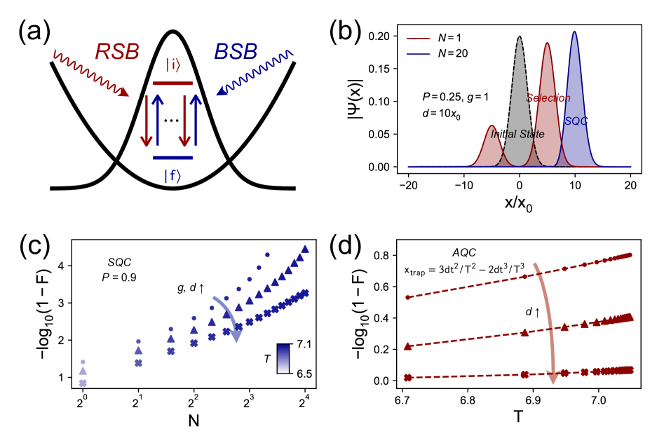
Figure 1: (a) Schematic diagram of SQC in trapped ion quantum platform using sequential selections (2), where two lasers are tuned to the first red and blue sideband to couple the internal spin states to the motional mode. Iterative pre-selection of the two-level system for $|i\rangle$ and post-selection for $|f\rangle$ (or vice versa) accumulates weak value on the position of the Gaussian-type apparatus, realizing SQC with the probability of $P=|\langle i|f\rangle|^{2N}$ after $N$ rounds without an ensemble of $N$ particles. (b) Final apparatus states for transporting a distance of $d=x_{0}$ with interaction strength $g=1$, where SQC achieves a fidelity of $F=|\langle\Psi(x,T)|\Psi_{G}\rangle|^{2}=0.995$ with $g\delta T=0.341$ and $N=20$. Selections (Superoscillating Quantum Control Induced By Sequential Selections) on the two-level system shift the initial ground state (grey) to final states by single shot selection (red) and $N=20$ rounds(blue) after $T=3.536$ and $6.830$, respectively. As a calibration, single-round selections show two non-overlapping red wave packets that cannot result in the unidirectional ion transport. The relevant dimensionless mass and trap frequency are $M=\nu=1$, and $P=0.25$. (c) Fidelity dependence on $N$ via SQC for transport distances of $d=7.5x_{0}$ (dot), $10x_{0}$ (triangle), and $15x_{0}$ (cross) with $g=0.75,~{}1,~{}1.5$, and $P=0.9$. (d) Fidelity dependence on $T$ via AQC for the same transport distances as in (c). We move the center of the trap by defining $x_{\text{trap}}=3dt^{2}/T^{2}-2dt^{3}/T^{3}$.

To realize SQC with the setup shown in Fig. 1(a), we apply $N$ rounds of sequential quantum-state pre- and post-selections by alternatively projecting the system into the initial state $|i\rangle$ and $|f\rangle$, and coupling the apparatus weakly to the system between two selections. The sequential selections on the system can exert a longstanding influence on the quantum state of apparatus, leading to the final state given by

$$|\Psi^{F}_{A}\rangle=|\langle f|i\rangle|^{N}\underbrace{\left[\cos\left(\frac{gT}{\hbar}\frac{\hat{p}}{N}\right)-i\sigma_{xw}\sin\left(\frac{gT}{\hbar}\frac{\hat{p}}{N}\right)\right]^{N}}_{=:f(p)}|\Psi(x)\rangle,~{}~{}$$ (2)

where $\sigma_{xw}=\langle f|\hat{\sigma_{x}}|i\rangle/\langle f|i\rangle$ is the weak value of $\hat{\sigma_{x}}$, $T$ is the total operation time, and $|\Psi(x)\rangle$ is the initial motional wave function of the apparatus. The sequential selections evolves the wave function by a superoscillating operator function $f(\hat{p})$ in Eq. (2). Mathematically, it allows the parameter $\sigma_{xw}>1$ and $\sigma_{xw}\in\mathcal{R}$, even though $\sigma_{xw}$ as a weak value can be complex in practice jozsa . The SO occurs with a low probability of $|\langle f|i\rangle|^{2N}$ since we discard the wave function and initialize the system once any selection on internal states fails. It accumulates a weak value on the apparatus by kicking its position $\delta x=gT\sigma_{xw}/N$ in each round, amplifying it by $N$ times without an ensemble of $N$ ions.

In addition to compensating force and inverse engineering Erik ; An ; transportreview , the SO described in Eq. (2) provides an alternative shortcut-to-adiabaticity transport by periodically kicking the particle without excitation. We can treat the motional wave function as the target since there is a system-apparatus duality, making the selections on the internal states the effective controller. To determine the cost of using SO, we need to analyze the relation between probabilities and transport distance and optimize the selections accordingly. A successful post-selection that projects an arbitrary state from $|i\rangle$ to $|f\rangle$, has a probability of $p=|\langle f|i\rangle|^{2}$. For our concern, to obtain a weak value of both real-valued and larger-than-one, we construct the two selected states

$$|i\rangle=\sqrt{\frac{1-\sqrt{1-p}}{2}}|0\rangle+\sqrt{\frac{1+\sqrt{1-p}}{2}}|1\rangle,$$

$$|f\rangle=\sqrt{\frac{1+\sqrt{1-p}}{2}}|0\rangle+\sqrt{\frac{1-\sqrt{1-p}}{2}}|1\rangle,$$ (3)

where $p$ is the probability of successful projection, which can result in an optimal weak value of $\sigma_{xw}=1/\sqrt{p}$. Therefore, the SQC protocol can shift the trapped ion by $d=gT/\sqrt{p}$, at the cost of $P=p^{N}$. At first glance, it may seem problematic because the displacement is independent of the number of selection $N$, and the total probability falls exponentially. That is, one can couple the internal states and the motional mode for the time interval of $T$ in a single shot of measurement. However, the coupling strength $gT$ maybe too large so that the coupling no longer evolves as a translation operator on the motional wave function. From an intuitive perspective, the post-selection on the system after evolving the system-apparatus Hamiltonian determined by $\langle f|\exp(-igT\hat{\sigma_{x}}\otimes\hat{p})|\Psi(x)\rangle|i\rangle$, splitting the apparatus to the cat state (or kitty-state when two packets are not well separated):

$$|\text{cat}\rangle=\frac{1+\sqrt{p}}{2\mathcal{N}}|\Psi(x-gT)\rangle+\frac{-1+\sqrt{p}}{2\mathcal{N}}|\Psi(x+gT)\rangle,$$ (4)

where $\mathcal{N}$ is the coefficient for normalization. Noteably, we present the exact final quantum state of the apparatus, which is applicable for measurements with arbitrary strengths, ranging from weak to strong coupling. The overlap between two wave packets is crucial to define the measurement transition, given by $\langle\Psi(x-gT)|\Psi(x+gT)\rangle=\exp(-\Gamma^{2})$, where $\Gamma=gT/(\sqrt{2}x_{0})$ is an interference factor. Using this, we derive the expected net shift of the apparatus:

$$\langle\delta x\rangle=\langle\text{cat}|x|\text{cat}\rangle=\frac{2\sqrt{p}gT}{1+p+\exp(-\Gamma^{2})(-1+p)},$$ (5)

which corresponds to the weak-valued readout $\sigma_{xw}gT=gT/\sqrt{p}$ asymptotically as $\Gamma\rightarrow 0$, while in the opposite limit of strong measurement $\Gamma\rightarrow\infty$, it results in a bizarre readout of $2\sqrt{p}gT/(1+p)$ that does not match the expectation value of $\hat{\sigma_{x}}$ in the initial or final state. More importantly, the net shift at weak measurement limit can be amplified when $p\rightarrow 1$. To preserve the unidirectional shift, we construct the SQC by periodically decoupling the system and the apparatus after every $\delta T=T/N$, ensuring each measurement is in the weak measurement regime. Fig. 1(b) plots the difference between single-shot measurement and SQC for a target distance of $d=10x_{0}$ with a low total probability of $P=0.25$ to increase result contrast.

In Fig. 1(c), we set the probability to $P=0.9$ and vary the number of selections from $N=1$ to $16$ to test the ideal performance of our protocol under different measurement strengths. We fix the operation time corresponding to $N$ in each set of settings by letting the coupling strength be proportional to the transport distance as (i): $g=0.75,~{}d=7.5x_{0}$, (ii): $g=1,~{}d=10x_{0}$, (iii): $g=1.5,~{}d=15x_{0}$. The results support our theory that the fidelity should increase with $N$ and decrease with transport distance.

We notice that the extra time cost (compared with $T=6.708$ for $N=1$) for SQC is not remarkable since the nonoverlapping wave packet on the left is almost negligible with near-parallel selection for $P\approx 1$. Furthermore, we highlight that the SQC converges to the lossless expectation value amplification (also the eigenvalue $\langle\hat{\sigma_{x}}\rangle=1$) with near parallel selection of the system states. This convergence bounds the quantum speed limit of lossless transport as $\dot{x}=g$. In this case, the apparatus (4) reduces to a single wave packet $|\Psi(x-gT)\rangle$, and equalizes the weak value $1/\sqrt{p}$ or the the previous bizarre readout $2\sqrt{p}/(1+p)$ in either limit. Alsom in Fig. 1(d), we benchmark our protocol by moving the center of the harmonic trap to the target with the following trajectory $x_{\text{trap}}=3dt^{2}/T^{2}-2dt^{3}/T^{3}$. $T=N\delta T$ is the operation time for the SQC of $N$ rounds. Our protocol significantly outperforms such adiabatic quantum control (AQC) in fidelity $F=|\langle\Psi(x,T)|\Psi_{G}\rangle|^{2}$, where $|\Psi_{G}\rangle$ is a Gaussian ground state at the target site, and prevails even when takingt the probability of the selections into account.

Speeding up adiabatic quantum search algorithm.— Now we generalize the superoscillating quantum control to include the angular parameters that characterize the wave function and enable the processing of quantum information. Similar to the weak value accumulation on the spatial parameter, the accumulation on the angular parameter amplifies the corresponding coefficient of the target basis. This is analogous to the adiabatic version of Grover’s algorithm haystack , searched for the target $|t\rangle$ from the database $|\Psi\rangle$ with a complexity of $\mathcal{O}(\sqrt{N_{G}})$ in the context of digitized quantum computing, where $N_{G}$ is the number of entries. This algorithm iteratively evolves the Grover’s operator $\hat{G}=U_{\Phi}U_{t}$, where the oracle operator $U_{t}=I-2|t\rangle\langle t|$ and the diffusion operator $U_{\Psi}=2|\Psi\rangle\langle\Psi|-I$ flip the phase of the wave function in the target subspace and the phase of the initial database, respectively. By decomposing $\hat{G}$ into a gate sequence, the algorithm rotates the wave function from the database to the target:

$$\hat{G}^{N}|\Psi\rangle=\sin\left(\frac{2N+1}{2}\theta\right)|t\rangle+\cos\left(\frac{2N+1}{2}\theta\right)|\tilde{t}\rangle.$$ (6)

We aim to implement an interaction Hamiltonian $H=g\hat{\sigma}\otimes\hat{J}$ that couples the system and the apparatus, where $\hat{\sigma}$ is the Pauli operator and $\hat{J}$ is the angular momentum. By sequentially selecting the system state, we can manipulate the quantum information encoded in angular parameters, resulting in the following SO on the apparatus

$$|\Psi_{A}^{F}\rangle=|\langle f|i\rangle|^{N}|\Psi(\theta/2+N\sigma_{w}g\delta T)\rangle,$$ (7)

where the interaction lasts for a duration of $\delta T=T/N$ in each sequence. If we define $g\delta T\sigma_{w}=\theta$, the SO is equivalent to Eq. (6). This oscillating quantum search requires both artificial design of selections, the angular momentum operator, and the implementation of the interaction Hamiltonian, which avoid decomposing the oracles in digitized quantum computing. In Fig. 2(a), we demonstrate the algorithm by using a two-qubit system, as a minimal quantum model that searches for the target state $|t\rangle=|0\rangle$ out of $N_{G}=2$ entries. Assuming that the initial database is $|\Psi\rangle=|+\rangle=\sin(\pi/4)|0\rangle+\cos(\pi/4)|1\rangle$, we can achieve a perfect query by setting $g\delta T\sigma_{yw}=\pi/4N$ instead of using the standard Grover’s algorithm. Accordingly, we use the spin-spin interaction for implementing the SQC, which is indeed the Heisenberg type $H_{\text{SQC}}=-g\hat{\sigma_{y}}\otimes\hat{\sigma_{y}}$ review2021 , when an auxiliary qubit is introduced as the controller (system). We add the relative phase term $\exp(-i\pi/2)$ on the coefficients of Eq. (Superoscillating Quantum Control Induced By Sequential Selections), and trade-off between the probability and weak value accumulation remains.

We hereby present a quantitative study comparing the energy cost of SQC with AQC. In the AQC approach, we evolve the time-dependent Hamiltonian $H(t)=[1-\lambda(t)]H_{i}+\lambda(t)H_{f}$, with $\lambda(t)$ ranging from zero to a certain value within the operation time. We use the type-I Hamiltonian as a benchmark for the specific quantum search stagrover , given by

$$H_{\textup{I}}(t) = (1-t/T)\Omega\hat{\sigma_{x}}+(t/T)\Delta\hat{\sigma_{z}},$$ (8)

with Rabi frequency $\Omega$, and the detuning $\Delta$. Additionally, we use the more general type-II Hamiltonian aqcgrover

$$H_{\textup{II}}(t) = (1-t/T)K(I-|\Psi\rangle\langle\Psi|)+(t/T)K(1-|t\rangle\langle t|),$$ (9)

as the baseline, where $K$ is a scaling coefficient. We evaluate the performance of SQC by measuring fidelities $F=|\langle\Psi(T)|t\rangle|^{2}$ on different $N$ with the same probability $P=0.9$ and coupling strength $g=1$ in Fig. 2(b). It is evident that the fidelity can be improved without increasing the operation time $T$ by using a larger Rabi frequency and detuning in the type-I Hamiltonian, or equivalently scaling up $K$ in the type-II Hamiltonian. Therefore, it is critical to define the energey cost energetic that bounds the input energy to the system for a fair comparison. We use the Frobenius norm of the total Hamiltonian to define the instantaneous cost of the evolution $\partial_{t}C=||H(t)||$, integrate and average it over the operation time as

$$C=\frac{1}{T}\int_{0}^{T}||H(t)||dt,$$ (10)

yielding $C_{\text{SQC}}=2g$ for the superoscillating quantum search. Assuming $\Omega=\Delta$, we derive the cost of type-I and type-II Hamiltonian as $C_{\textup{I}}=\Omega[2\sqrt{2}-\log(-1+\sqrt{2})+\log(1+\sqrt{2})]/4$ and $C_{\textup{II}}=K[4+3(-\log 1+\log 3)]/8$, respectively. Fig. 2(c) shows the energy cost of adiabatic algorithms to SQC, along with the fidelities of both types of Hamiltonian for adiabatic quantum search within $T$, corresponding to selections of $N$ rounds. Numerical results prove that SQC dramatically accelerates the adiabatic Grover’s algorithm, even if both probabilistic and energetic cost are considered. We analyze its extension to arbitrary databases by applying the multi-qubits in the Supplementary Material supplementary . The model is physically feasible in the trapped ion platform, where Mølmer-Sørensen gates serve naturally as analog simulators for the interaction.

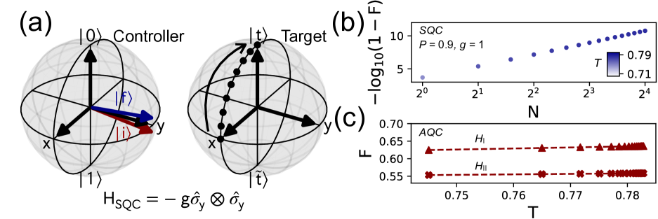
Figure 2: (a) Schematic diagram of quantum search algorithm using SQC (7). $N=8$ rounds of selections on the controller qubit, driven by the spin-spin interaction Hamiltonian $H_{\text{SQC}}=-g\hat{\sigma_{y}}\otimes\hat{\sigma_{y}}$, rotate the target qubit from the initial database $|\Psi\rangle=|+\rangle$ to the target $|t\rangle=|0\rangle$. (b) Fidelity dependence on $N$ via SQC. The probability of SQC and coupling strength are set to $P=0.9$ and $g=1$, respectively. (c) Fidelity dependence on $T$ via AQC. The energetic cost is bounded, and the AQC Hamiltonians (8) (red triangle), (9) (red cross) are evolved for $T$ that depends on the rounds of selections in SQC algorithm.

Possible experimental implementation.— Both examples in the ideal simulations approach the lossless SO in the limit of large $N$. To evaluate the protocol in a laboratory environment, we generalize it to open quantum systems governed by the Lindblad master equation. We account for imperfect selections that can introduce atomic loss and quantum noises, reducing fidelity by a fixed proportion $P_{\text{error}}$. These mechanisms can create a trade-off between the fidelity and the number of selections, where the fidelity reaches a maximum and then decreases as $N$ increases beyond a critical value. Note that the trade-off of the first type, induced by quantum noises, does not necessarily exist in all cases. As $N$ increases, the protocol preserves the better property of SQC, which improves fidelity with extra operation time, while reducing fidelity as quantum noises affect the system more. Whether this trade-off exists depends on which factor dominates, extra fidelity gain or loss.

To characterize the dephased two-level system (internal state) and damped quantum harmonic oscillator (motional mode) involved in the ion transport task, we use the collapse operators $C_{\text{TLS}}=\sqrt{\gamma}\hat{\sigma_{z}}$, $C_{\text{HO}}=\sqrt{\gamma}\hat{a}~{},\sqrt{\gamma}\hat{a}^{\dagger}$, respectively. Solving the Lindblad master equation enables us to obtain the fidelity in the formulation of density matrix approach. As a result of the damping, the expected shift of the damped apparatus is smaller than that of the ideal apparatus. As shown in Fig. 3(a), we set the same dephasing rate and damping rate to $\gamma=0.01$, and the additional fidelity loss per selection to $P_{\text{error}}=5\times 10^{-3}$. Although the only trade-off in this parameter setting is induced by imperfect projection, the trade-off of the first type can be observed at a small critical $N$ by tuning down the probability of SQC. In the quantum search algorithm, we impose local dephasing on the control qubit (system) and target qubit (apparatus) by $C_{\text{TLS}}=\sqrt{\gamma}\hat{\sigma_{z}}$, resulting in a decrease in fidelity due to purity loss. As calibrations, the evaluation of the algorithm with the same parameters is shown in Fig. 3(b,c), which confirms the existence of a trade-off mechanisms of two types.

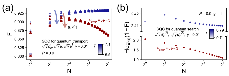
Figure 3: (a) Fidelity vs. $N$ in SQC-based quantum transport, with quantum noises characterized by dephasing and damping rates of $\gamma=0.01$. Simulation results for the open quantum system are multiplied by $1-P_{\text{error}}=0.995$ after each selection (red markers) to mimic atomic loss induced by imperfect projections. Parameters and markers are the same as in Fig. 1(c). (b) Fidelity vs. $N$ in SQC-based quantum search, with local dephasing modeled by $C_{\text{TLS}}=\sqrt{\gamma}\hat{\sigma_{z}}$ on the controller and target qubits. Results are shown for perfect (blue) and imperfect (red) projections with the same settings as in (a) and in Fig. 2(b).

Conclusion and outlook.— In summary, we have introduced a general SQC framework and demonstrated its efficiency in two applications with trapped ions. Our approach utilizes pre- and post-selections of the system to achieve optical projection design, and SQC for atomic non-adiabatic transport and the quantum search problem. We have shown that SQC can speed up conventional adiabatic control, offering a promising alternative toward shortcuts to adiabaticity. Numerical simulations demonstrate that SQC has advantages in terms of energy cost, even when considering the probability of occurrence. We have also extended the SQC protocol to open quantum systems, where noise affects its performance, resulting in two types of trade-offs between selections and fidelity.

While our focus is on the trapped ion system, insights can be gained from the cold atoms in spin-dependent optical potentials Martin , and electrons in semiconductor quantum dots Sherman . Additionaly, our work can be extended to coherent matter-wave splitting, as we have presented the analytical formulation of the apparatus after post-selection. Furthermore, SQC for collective behaviour has applications in the emergence or suppression of superradiant phase transition in the Dicke model dicke . We believe that SQC can provide a deeper understanding of quantum foundations and offer potential for various quantum technologies.

Supplemental Material: Superoscillating Quantum Control Induced By Sequential Selections

.1 Bichromatically excited single trapped ion for atomic transport

In the Lamb-Dicke regime, the criteria $\eta\sqrt{\langle(\hat{a}+\hat{a}^{\dagger})^{2}\rangle}\ll 1$ should hold during the operation time. the Lamb-Dicke Hamiltonian contains the red sideband and blue sideband as resonances. The first red sideband $\delta=-\nu$ reads

$$H_{\text{rsb}}=\frac{\hbar}{2}\Omega\eta\left[\hat{a}\hat{\sigma}_{+}\exp\left(i\phi_{r}\right)+\hat{a}^{\dagger}\hat{\sigma}_{-}\exp\left(-i\phi_{r}\right)\right],$$ (S1)

where $\phi_{r}$ is the phase of the laser, giving the transition $|n\rangle|g\rangle\leftrightarrow|n-1\rangle|e\rangle$ with the effective Rabi frequency $\Omega\sqrt{n}\eta$. It couples the internal states and the motional mode of the single trapped ion. Similarly, we write down the first blue sideband $\delta=-\nu$ as

$$H_{\text{bsb}}=\frac{\hbar}{2}\Omega\eta\left[\hat{a}^{\dagger}\hat{\sigma}_{+}\exp\left(i\phi_{b}\right)+\hat{a}\hat{\sigma}_{-}\exp\left(-i\phi_{b}\right)\right],$$ (S2)

giving another transition $|n\rangle|g\rangle\leftrightarrow|n+1\rangle|e\rangle$ with the effective Rabi frequency $\Omega\sqrt{n+1}\eta$. These resonances lead to the well-known Jaynes-Cummings and anti-Jaynes-Cummings Hamiltonian, respectively. We implement the light-matter interaction by turning on the bichromatic laser, and reduce the Lamb-Dicke Hamiltonian to

$$H_{\text{bic}}=H_{\text{rsb}}+H_{\text{bsb}}=-i\frac{\hbar\Omega}{2}\eta\hat{\sigma_{x}}\left(\hat{a}-\hat{a}^{\dagger}\right),$$ (S3)

with $\phi_{r}=-\pi/2$ and $\phi_{r}=\pi/2$. By substituting $\hat{a}=\sqrt{M\nu/2\hbar}(\hat{x}+i\hat{p}/M\nu)$ and $\hat{a}^{\dagger}=\sqrt{M\nu/2\hbar}(\hat{x}-i\hat{p}/M\nu)$ into (S3), we derive the interaction Hamiltonian in the main text as $H=g\hat{\sigma_{x}}\otimes\hat{p}$, where $g=\eta\Omega x_{0}$ and $x_{0}=\sqrt{\hbar/2M\nu}$.

.2 Weak-to-strong quantum measurement, weak value, and expectation value

We present a detailed calculation of the weak-to-strong quantum measurement, in order to verify the necessity of using SO instead of a single shot of strong measurement. One chooses the states for pre-selection and post-selection, and express them in the eigenbasis of the operator for measurement, e.g.,

$$|i\rangle=a_{0}|+\rangle+a_{1}|-\rangle,$$

$$|f\rangle=\tilde{a_{0}}|+\rangle+\tilde{a_{1}}|-\rangle,$$ (S4)

if we measure the weak value of $\hat{\sigma_{x}}$. Such quantum measurement process with arbitrary measurement strength exacly reads

$$\langle f|\exp(-igT\hat{\sigma_{x}}\otimes\hat{p})|i\rangle\otimes|\Psi(x)\rangle$$ (S5)

$$= c_{0}|\Psi(x-gT)\rangle+c_{1}|\Psi(x+gT)\rangle,$$

where $c_{0}=a_{0}\tilde{a_{0}}^{*}$ and $c_{1}=a_{1}\tilde{a_{1}}^{*}$. We can renormalize these two wave packets into a cat state as

$$|\text{cat}\rangle = \frac{c_{0}|\Psi(x-gT)\rangle+c_{1}|\Psi(x+gT)\rangle}{\sqrt{[c_{0}^{*}\langle\Psi(x-gT)|+c_{1}^{*}\langle\Psi(x+gT)][c_{0}|\Psi(x-gT)\rangle+c_{1}|\Psi(x+gT)\rangle]}},$$ (S6)

$$= \frac{c_{0}|\Psi(x-gT)\rangle+c_{1}|\Psi(x+gT)\rangle}{\sqrt{|c_{0}|^{2}+|c_{1}|^{2}+(c_{0}^{*}c_{1}+c_{0}c_{1}^{*})\langle\Psi(x-gT)|\Psi(x+gT)\rangle}}.$$

We quantify the quantum interference in the measurement by $\langle\Psi(x-gT)|\Psi(x+gT)\rangle=\exp(-\Gamma^{2})$, and define the interference factor $\Gamma=gT/(\sqrt{2}x_{0})$. We obtain the measurement outcome by calculating the central position shift from the initial Gaussian ground state to the cat state

$$\delta x=\langle\text{cat}|\hat{x}|\text{cat}\rangle=\frac{(|c_{0}|^{2}-|c_{1}|^{2})gt}{|c_{0}|^{2}+|c_{1}|^{2}+(c_{0}^{*}c_{1}+c_{0}c_{1}^{*})\exp(-\Gamma^{2})}.$$ (S7)

We have $\langle\delta x\rangle|_{\Gamma\rightarrow 0}=\frac{(|c_{0}|^{2}-|c_{1}|^{2})gt}{|c_{0}|^{2}+|c_{1}|^{2}+c_{0}^{*}c_{1}+c_{0}c_{1}^{*}}=\sigma_{xw}gt$ in the weak-coupling regime. However, $\langle\delta x\rangle|_{\Gamma\rightarrow\infty}=\frac{(|c_{0}|^{2}-|c_{1}|^{2})gt}{|c_{0}|^{2}+|c_{1}|^{2}}$ does not always amplifies the expectation value $\langle f|\hat{\sigma_{x}}|f\rangle$ in the strong-coupling regime. In our main text, we choose the optimal selection for atomic transport

$$|i\rangle = \sqrt{\frac{1-\sqrt{1-p}}{2}}|0\rangle+\sqrt{\frac{1+\sqrt{1-p}}{2}}|1\rangle,$$

$$|f\rangle = \sqrt{\frac{1+\sqrt{1-p}}{2}}|0\rangle+\sqrt{\frac{1-\sqrt{1-p}}{2}}|1\rangle,$$ (S8)

which the weak value is $1/\sqrt{p}$ and the expectation value $\langle f|\hat{\sigma_{x}}|f\rangle=\sqrt{p}$. However, in the strong measurement limit we observe a readout of $\frac{2\sqrt{p}}{1+p}$ instead. To equalize the measurement readout and the expectation value, we artificially design a pre-selection and post-selection, e.g.,

$$|i\rangle=|0\rangle,|f\rangle=\sqrt{p}|0\rangle+\sqrt{1-p}|1\rangle,$$ (S9)

which its weak value and expectation value are $\frac{\sqrt{1-p}}{\sqrt{p}}$ and $2\sqrt{-(-1+p)p}$, that the latter one agrees with the measurement readout in the strong-coupling limit. We show the weak-to-strong transition under both settings in Fig. S1.

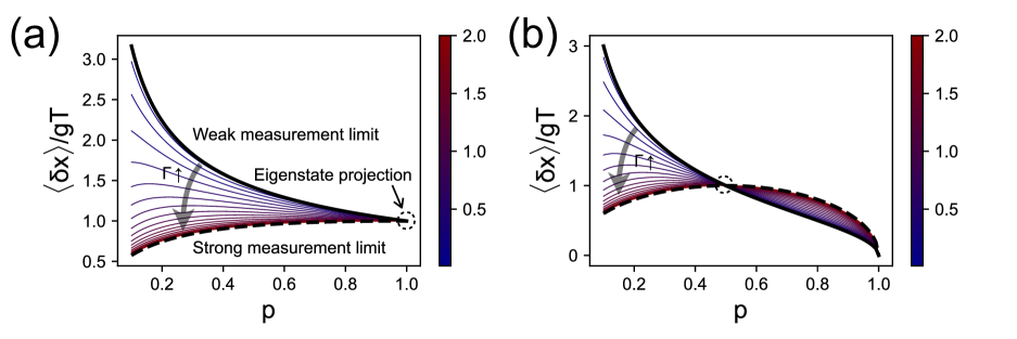
Figure S1: The relative central position shift from the initial Gaussian state to the cat state $\langle\delta x\rangle/gT$ as a function of the selection probability $p$ with different measurement strength characterized by the interference factor $\Gamma=gt/(\sqrt{2}x_{0})$. (a) We set the states for pre-selection and post-selection be $|i\rangle=\sqrt{\frac{1-\sqrt{1-p}}{2}}|0\rangle+\sqrt{\frac{1+\sqrt{1-p}}{2}}|1\rangle$ and $|f\rangle=\sqrt{\frac{1+\sqrt{1-p}}{2}}|0\rangle+\sqrt{\frac{1-\sqrt{1-p}}{2}}|1\rangle$, respectively. The thick black solid curve denotes the weak value readout $\sigma_{xw}=1/\sqrt{p}$ in the weak measurement limit $\Gamma\rightarrow 0$. The thick black dashed curve denotes the bizzare readout $2\sqrt{p}/(1+p)$ in the strong measurement limit $\Gamma\rightarrow\infty$, which is not in accordance with the expectation value $\langle f|\hat{\sigma_{x}}|f\rangle=\sqrt{p}$. Other possible readout curves lie between them in the color according to the value of $\Gamma$. We circle the point for eignenstate projection of $|+\rangle$, where the weak and strong measurement meet each other losslessly. (b) We set the states for pre-selection and post-selection be $|i\rangle=|0\rangle$ and $|f\rangle=\sqrt{p}|0\rangle+\sqrt{1-p}|1\rangle$, respectively, for equalizing the expectation value and the readout in the strong measurement limit as $2\sqrt{-(-1+p)p}$. The weak measurement output is $\frac{\sqrt{1-p}}{\sqrt{p}}$. Here the eigenstate projection has a probability of $0.5$. Other configurations definitions are the same as those in the previous subfigure.

.3 Analog simulation of quantum search with Mølmer-Sørensen gate

In the maintext, we propose the YY interaction for recovering Grover’s search with sequential selections. As we mentioned, we can use two trapped ion to perform an analog simulation. We excite them bichromatically, which the Hamiltonian reads

$$H_{\text{bic}}(t)=\frac{\hbar}{2}\Omega\left(\hat{\sigma}_{+}^{(1)}+\hat{\sigma}_{+}^{(2)}\right)\left\{1+i\eta\left[\hat{a}\exp(-i\nu t)+\hat{a}^{\dagger}\exp(i\nu t)\right]\right\}\left[\exp(-i\delta t)+\exp(i\delta t)\right]+\text{H.c.},$$ (S10)

exactly yielding the propagator

$$U_{\text{bic}}(t)=\hat{D}\left\{\frac{\eta\Omega}{\epsilon}\left[\exp(i\epsilon t)-1\right]\hat{J_{y}}\right\}\exp\left\{i\left[\frac{\eta^{2}\Omega^{2}}{\epsilon}t-\frac{\eta^{2}\Omega^{2}}{\epsilon^{2}}\sin\left(\epsilon t\right)\right]\hat{J_{y}^{2}}\right\},$$ (S11)

where the laser detuning from the motional sidebands is $\epsilon=\nu-\delta$, $\hat{D}(\alpha)$ is the displacement operator, and the collective spin operator is $\hat{J_{y}}=\hat{s_{y}}^{(1)}+\hat{s_{y}}^{(2)}$. The displacement operator vanishes when $t_{\text{MS}}=2\pi/\epsilon$. Thus, the propagator is the action of an effective Hamiltonian $H=-\hbar(\eta^{2}\Omega^{2}/\epsilon)\hat{s_{y}}^{(1)}\otimes\hat{s_{y}}^{(2)}$, which effectively entangling the controller qubit $\hat{s_{y}}^{(1)}$ and the target qubit $\hat{s_{y}}^{(2)}$. For other initial databases, one can always find an axis for rotation, requiring $\hat{\sigma}_{\phi}^{1}\otimes\hat{\sigma}_{\phi}^{2}$ interaction, where $\hat{\sigma}_{\phi}=\cos\phi\hat{\sigma_{x}}+\sin\phi\hat{\sigma_{y}}$, which is also feasible with different phases of the laser. Note that the analog simulation does not satisfies the energetic bound in the main text since it is not a direct realization of YY interaction.

.4 Construction of general angular momentum operator

For entries $N_{G}>2$, it takes multiple qubits as the database to encode the quantum information. Thus, the physical picture of Bloch sphere in the minimal model is no longer valid, requiring a generalization of the rotation in the Hilbert space of higher dimension. Let us assume that the initial database for quantum search of target state $|t\rangle$ reads

$$|\Psi\rangle=\sin\frac{\theta}{2}|t\rangle+\cos\frac{\theta}{2}|\tilde{t}\rangle,$$ (S12)

where $|\tilde{t}\rangle=\sum_{N_{G}-1}c_{i}|i\rangle$ is complementary basis in the superposition of all other entires. To realize the SO for quantum search, we need to construct a general angular momentum $\hat{J}$ that rotates the parameterized wave function by $\exp(-i\phi\hat{J})|\Psi(\theta/2)\rangle=|\Psi(\theta/2+\phi)\rangle$. We can still construct such angular momentum by mimicking the rotation in the minimal model. For example, we can rotate the wave function toward the target about an effective Y-axis if the amplitudes of all bases are real. We denote the effective plus state and minus state by

$$|\tilde{+}\rangle = \frac{\sqrt{2}}{2}|t\rangle+\frac{\sqrt{2}}{2}|\tilde{t}\rangle,$$

$$|\tilde{-}\rangle = \frac{\sqrt{2}}{2}|t\rangle-\frac{\sqrt{2}}{2}|\tilde{t}\rangle,$$ (S13)

leading to the general angular momentum operator

$$\hat{J_{y}}=-\frac{i}{2}(|\tilde{-}\rangle\langle\tilde{+}|-|\tilde{+}\rangle\langle\tilde{-}|),$$ (S14)

which rotates the parameterized wave function as we desire.