On well-posedness of $\alpha$-SQG equations in the half-plane

Abstract

We investigate the well-posedness of $\alpha$-SQG equations in the half-plane, where $\alpha=0$ and $\alpha=1$ correspond to the 2D Euler and SQG equations respectively. For $0<\alpha\leq 1/2$, we prove local well-posedness in certain weighted anisotropic Hölder spaces. We also show that such a well-posedness result is sharp: for any $0<\alpha\leq 1$, we prove nonexistence of Hölder regular solutions (with the Hölder regularity depending on $\alpha$) for initial data smooth up to the boundary.

1 Introduction

1.1 Generalized SQG equations

In this paper, we are concerned with the Cauchy problem for the inviscid $\alpha$-surface quasi-geostrophic ($\alpha$-SQG) equations on the right half plane $\mathbb{R}^{2}_{+}=\{(x_{1},x_{2})\in\mathbb{R}^{2};x_{1}>0\}$

$$\left\{\begin{aligned} &\partial_{t}\theta+u\cdot\nabla\theta=0,\\ &u=-\nabla^{\perp}(-\Delta)^{-1+\frac{\alpha}{2}}\theta,\end{aligned}\right. \alpha$$ (-SQG)

for $0\leq\alpha\leq 1$. For notational simplicity, throughout this paper we shall normalize the constant in a way that the Biot–Savart law becomes

$$\begin{split}u(t,x)=\int_{\mathbb{R}^{2}_{+}}\left[\frac{(x-y)^{\perp}}{|x-y|^{2+\alpha}}-\frac{(x-\tilde{y})^{\perp}}{|x-\tilde{y}|^{2+\alpha}}\right]\theta(t,y)\,\mathrm{d}y,\end{split}$$ (1.1)

where $\tilde{y}:=(-y_{1},y_{2})$ for $y=(y_{1},y_{2})$.

In the last decade, the $\alpha$-SQG equations (either with or without dissipation) in domains with boundaries have attracted a lot of attention. The constructed solutions were either $L^{p}$ weak solutions, patch solutions, or solutions that vanish on the boundary. Below we summarize the previous literature on well-posedness of solutions.

• Weak solutions: For the generalized SQG (or SQG) equation, when the equation is set up in a domain with a boundary, global existence of weak solution in $L^{\infty}_{t}L^{2}_{x}$ was established in [5, 20, 4]. We refer to [21, 19, 1] for the existence of weak solutions in $\mathbb{R}^{2}$ and [2, 13, 3] for the non-uniqueness of the weak solutions. Existence results of weak solutions in $\mathbb{R}^{2}$ can be directly applied to give weak solutions in $\mathbb{R}^{2}_{+}$ by considering solutions which are odd in one variable.

• Patch solutions: For the 2D Euler equation on the half plane, global existence of $C^{1,\gamma}$ patch solutions was shown in [8, 9, 17]. For the $\alpha$-SQG equations on the half plane, local well-posedness of $H^{3}$-patch solutions for $\alpha\in(0,\frac{1}{12})$ was established in [18], and it was shown in [17] that such patch solution can form a finite time singularity for this range of $\alpha$. Later, [12] extended the local well-posedness and finite-time singularity results to $\alpha\in(0,\frac{1}{6})$ for $H^{2}$-patch solutions. The creation of a splash-like singularity was ruled out in the works [14, 16]. We also refer to [6] for stability of the half-plane patch stationary solution.

To the best of our knowledge, in the literature there has been no local well-posedness results for strong solutions of ($\alpha$-SQG) which do not vanish on the boundary. The difficulty is mainly caused by the fact that when $\theta$ do not vanish on the boundary, even if it is smooth, the regularity of the velocity field $u$ becomes worse as we get closer to the boundary, and $u$ is only $C^{1-\alpha}$ near the boundary. A closer look reveals that the two components of $u$ have different regularity properties. This motivates us to introduce an anisotropic functional space, which turns out to be crucial for us to establish the local-wellposedness result.

While we were finalizing the paper, a preprint by Zlatoš [22] appeared where the well-posedness problem is studied in a very similar setting, and the same type of anisotropic weighted space was discovered independently. A detailed discussion can be found in Remark 1.1 and the end of Section 1.2.

1.2 Main Results

For any $0<\beta\leq 1$, we introduce the space $X^{\beta}=X^{\beta}(\overline{\mathbb{R}^{2}_{+}})$, which is a subspace of $C^{\beta}(\overline{\mathbb{R}^{2}_{+}})$ with anisotropic Lipschitz regularity in space: we say $f\in X^{\beta}$ if it belongs to $C^{\beta}$, differentiable almost everywhere, and satisfies

$$\begin{split}\|f\|_{X^{\beta}}:=\|f\|_{C^{\beta}}+\|x_{1}^{1-\beta}\partial_{1}f\|_{L^{\infty}}+\|\partial_{2}f\|_{L^{\infty}}<\infty.\end{split}$$ (1.2)

The Hölder norm is defined by

$$\begin{split}\|f\|_{C^{\beta}}:=\|f\|_{L^{\infty}}+\sup_{x\neq x^{\prime}}\frac{|f(x)-f(x^{\prime})|}{|x-x^{\prime}|^{\beta}}.\end{split}$$ (1.3)

For simplicity, we only deal with the functions $f$ that are compactly supported in a ball of radius $O(1)$, so that we have $X^{\beta}\subset X^{\gamma}$ if $\beta\geq\gamma$. In general, one may replace the weight $x_{1}^{1-\beta}$ by something like $(x_{1}/(1+x_{1}))^{1-\beta}$.

It turns out that, in the regime $\alpha\in(0,\frac{1}{2}]$, the $\alpha$-SQG equation is locally well-posed in $X^{\beta}_{c}$. In the following theorem we prove the local well-posedness result, and also establish a blow-up criterion: if the solution in $X^{\beta}_{c}$ cannot be continued past some time $T<\infty$, then $\|\partial_{2}\theta(t,\cdot)\|_{L^{\infty}}$ must blow up as $t\to T$.

Theorem A.

Let $\alpha\in(0,\frac{1}{2}]$ and $\beta\in[\alpha,1-\alpha]$. Then ($\alpha$-SQG) is locally well-posed in $X^{\beta}_{c}$: for any $\theta_{0}\in X^{\beta}_{c}$, there exist $T=T(\|\theta_{0}\|_{X^{\alpha}},|{\mathrm{supp}}\,\theta_{0}|)>0$ and a unique solution $\theta$ to ($\alpha$-SQG) in the class $\mathrm{Lip}([0,T);L^{\infty})\cap L^{\infty}([0,T);X^{\beta}_{c})\cap C([0,T);C^{\beta^{\prime}})$ for any $0<\beta^{\prime}<\beta$. Furthermore, if $T<\infty$, then $\lim_{t\to T}\|\partial_{2}\theta(t,\cdot)\|_{L^{\infty}}\gtrsim(T-t)^{-\eta}$ holds for any $\eta\in(0,1)$.

Remark 1.1.

(Finite-time singularity formation in $X^{\beta}_{c}$). For $\alpha\in(0,\frac{1}{3})$, one can follow the same argument in [12, 17] to construct a $\theta_{0}\in C^{\infty}_{c}(\overline{\mathbb{R}^{2}_{+}})$ where the solution leaves $X^{\beta}_{c}$ in finite time. To show this, let us start with the initial data $1_{D_{0}}$ in [12, 17], where $D_{0}$ consists of two disjoint patches symmetric about the $x_{1}$ axis. (In our setting they are symmetric about the $x_{2}$ axis, since our domain is the right half plane.) We then set our initial data $\theta_{0}\in C^{\infty}_{c}(\overline{\mathbb{R}^{2}_{+}})$ such that $\theta_{0}\equiv 1$ in $D_{0}$, $\theta_{0}\geq 0$ in $\overline{\mathbb{R}^{2}_{+}}$, and $\theta_{0}\equiv 0$ on the $x_{1}$-axis. Assuming a global-in-time solution in $X^{\beta}$, on the one hand we have $\theta(t,\cdot)\equiv 0$ on the $x_{1}$-axis for all time by symmetry. On the other hand, one can check that all the estimates in [12, 17] on $u$ still hold, thus the set $\{\theta(t,\cdot)=1\}$ would touch the origin in finite time, leading to a contradiction.

For $\alpha>\frac{1}{3}$, significantly new ideas are needed to prove the singularity formation. In the very recent preprint by Zlatoš [22], he used some more precise and delicate estimates to improve the parameter regime to cover the whole range $\alpha\in(0,\frac{1}{2}]$ where the equation is locally well-posed.

Finally, we point out that the blow-up criteria in Theorem A implies that at the blow-up time $T$, we must have $\lim_{t\to T}\|\partial_{2}\theta(t,\cdot)\|_{L^{\infty}}=\infty$. It would be interesting to figure out what is the exact regularity of the solution at the blow-up time.

As a consequence of Theorem A, if the initial data is smooth and compactly supported in $\mathbb{R}^{2}_{+}$, there is a unique local solution in $L^{\infty}([0,T);X^{1-\alpha}_{c})$. Our second main result shows that this regularity is sharp, even for $C^{\infty}_{c}$-data. In fact, for all $C^{\infty}_{c}$ initial data that do not vanish on the boundary, we show that the $C^{\beta}$-regularity of the solution is instantaneously lost for all $\beta>1-\alpha$.

Theorem B.

Let $\alpha\in(0,\frac{1}{2}]$ and assume $\theta_{0}\in C^{\infty}_{c}(\overline{\mathbb{R}^{2}_{+}})$ does not vanish on the boundary. Then, the local-in-time solution $\theta$ to ($\alpha$-SQG) given by Theorem A does not belong to $L^{\infty}([0,\delta];C^{\beta}(\overline{\mathbb{R}^{2}_{+}}))$ for any $\beta>1-\alpha$ and $\delta>0$.

Remark 1.2.

The condition on the initial data necessary for illposedness in Theorem B can be relaxed to

$$\theta_{0}(x_{0})\neq 0,\qquad\limsup_{x\to x_{0},x\in\partial\mathbb{R}^{2}_{+}}\frac{|\theta_{0}(x_{0})-\theta_{0}(x)|}{|x_{0}-x|}>0$$

for some $x_{0}\in\partial\mathbb{R}^{2}_{+}$.

Our last main result, which deals with the case $\alpha>1/2$, shows that there is nonexistence of solutions not only in $X^{\alpha}_{c}$ but even in $C^{\alpha}$.

Theorem C.

Let $\alpha\in(\frac{1}{2},1]$ and assume $\theta_{0}\in C^{\infty}_{c}(\overline{\mathbb{R}^{2}_{+}})$ does not vanish on the boundary. Then, there is no solution to ($\alpha$-SQG) with initial data $\theta_{0}$ belonging to $L^{\infty}([0,\delta];C^{\alpha}(\overline{\mathbb{R}^{2}_{+}}))$ for any $\delta>0$.

Our main results are summarized in Figure 1. Namely, for $\alpha\in(0,1]$ and $\beta\in[0,1]$, we have the following three distinct regimes:

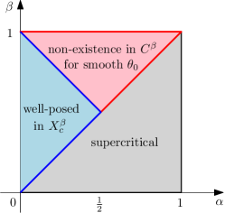
Figure 1: Illustration of well-posedness result of $\alpha$-SQG in $X^{\beta}_{c}$ spaces (in blue color), and non-existence results in $C^{\beta}$ for smooth initial data (in red color).

• The “wellposed” region is given by $\{0<\alpha\leq 1/2,\alpha\leq\beta\leq 1-\alpha\}$: note that the boundary points are included (Theorem A). The case $\beta=\alpha$ with $\alpha>0$ is especially interesting since it is known that $\alpha$-SQG equations are known to be illposed in the critical space $C^{\alpha}$ (and also in $H^{1+\alpha}$) in $\mathbb{R}^{2}$ ([15, 7, 10]). On the other hand, our result shows that when $\alpha\leq 1/2$, we have well-posedness for datum which behaves like $\theta_{0}(x)\sim\mathrm{const}+x_{1}^{\alpha}$ near the boundary $\{x_{1}=0\}$, which is exactly $C^{\alpha}$ and not better in the scale of Hölder spaces.

• On the other hand, the “illposed” region is given by $\{1/2<\beta\leq 1,1-\beta<\alpha\leq\beta\}$ for any given smooth and compactly supported initial data that do not vanish on the boundary (Theorems B and C). Note that the illposedness is proved not just in $X^{\beta}$ but in $C^{\beta}$. Indeed, if we consider any singular initial data $\theta_{0}\in C^{\alpha}_{c}(\overline{\mathbb{R}^{2}_{+}})$ with

  $$\theta_{0}(x_{0})\neq 0,\qquad\limsup_{x\to x_{0},x\in\partial\mathbb{R}^{2}_{+}}\frac{|\theta_{0}(x_{0})-\theta_{0}(x)|}{|x_{0}-x|^{\alpha}}>0$$

  for some $x_{0}\in\partial\mathbb{R}^{2}_{+}$, it is not hard to prove that ($\alpha$-SQG) are ill-posed in the critical Hölder space.

• Lastly, the regime $\beta<\alpha$ is “supercritical” with respect to the scaling of the $\alpha$-SQG equations; local well-posedness in $C^{\beta}$ (or even in $X^{\beta}$) is not expected, even in the whole space case $\mathbb{R}^{2}$. There have been several exciting developments in this regime: see [11, 7].

In the very recent preprint by Zlatoš [22], the local well-posedness of solutions was established in the same regime of parameters as our Theorem A. Compared to our work, [22] obtained ill-posedness in $X^{\beta}$ for broader parameters, covering both our ill-posed regime and supercritical regime. The idea was to construct some Lipschitz initial data of series form and to show that such initial data leaves $X^{\beta}$ immediately. Our ill-posedness result in Theorem B and C only deals with the red set in Figure 1, but it holds for more general initial data: namely, for every smooth initial data that does not vanish on the boundary, we show that the solution must leave $C^{\beta}$ immediately (recall that $X^{\beta}$ is a subset of $C^{\beta}$).

1.3 Outline of the paper

The remainder of this paper is organized as follows. In Section 2, we collect a few key estimates for the velocity. The proof of well-posedness (Theorem A) is given in Section 3. Lastly, we prove nonexistence results (Theorems B and C) in Section 4.

Acknowledgments

IJ has been supported by the Samsung Science and Technology Foundation under Project Number SSTF-BA2002-04. YY is partially supported by the NUS startup grant A-0008382-00-00 and MOE Tier 1 grant A-0008491-00-00.

2 Estimates on the velocity

In this section, we collect a few “frozen-time” estimates on the velocity.

2.1 Key Lemma

The following statement shows the precise regularity of the velocity under the assumption $\theta\in X^{\alpha}$.

Lemma 2.1.

Let $\alpha\in(0,1)$ and $\theta:\overline{\mathbb{R}^{2}_{+}}\to\mathbb{R}$ with ${\mathrm{supp}}\,\theta\subset B(0;1)$ and $|x_{1}^{1-\alpha}\partial_{1}\theta(x)|+|\partial_{2}\theta(x)|\leq C$ for some $C>0$. Then, the velocity $u=-\nabla^{\perp}(-\Delta)^{-1+\frac{\alpha}{2}}\theta$ satisfies

$$\begin{split}\|u_{1}\|_{C^{1,1-\alpha}(\overline{\mathbb{R}^{2}_{+}})}+\|\partial_{2}u_{2}\|_{C^{1-\alpha}(\overline{\mathbb{R}^{2}_{+}})}+\|\partial_{1}(u_{2}-U_{2})\|_{L^{\infty}(\overline{\mathbb{R}^{2}_{+}})}\leq C\left(\|x_{1}^{1-\alpha}\partial_{1}\theta\|_{L^{\infty}(\mathbb{R}^{2}_{+})}+\|\partial_{2}\theta\|_{L^{\infty}(\mathbb{R}^{2}_{+})}\right)\end{split}$$ (2.1)

where

$$\begin{split}U_{2}(x):=-\frac{2}{\alpha}\int_{-\infty}^{\infty}\frac{\theta(0,y_{2})}{|x-(0,y_{2})|^{\alpha}}\,\mathrm{d}y_{2}.\end{split}$$ (2.2)

Furthermore, $U_{2}$ satisfies

$$\begin{split}\|\partial_{2}U_{2}\|_{L^{\infty}({\mathbb{R}^{2}_{+}})}\leq C\|\partial_{2}\theta\|_{L^{\infty}(\mathbb{R}^{2}_{+})}\end{split}$$ (2.3)

and

$$\begin{split}\left|\partial_{1}U_{2}(x)-C_{\alpha}x_{1}^{-\alpha}\theta(0,x_{2})\right|\leq Cx_{1}^{1-\alpha}\|\partial_{2}\theta\|_{L^{\infty}}\end{split}$$ (2.4)

where

$$\begin{split}C_{\alpha}:=2\int_{\mathbb{R}}\frac{\mathrm{d}z}{(1+z^{2})^{\alpha/2+1}}.\end{split}$$ (2.5)

In particular, in the region $\{x_{1}\geq L\}$, we have $\|u\|_{Lip}\leq CL^{-\alpha}\big{(}\|x_{1}^{1-\alpha}\partial_{1}\theta\|_{L^{\infty}(\mathbb{R}^{2}_{+})}+\|\partial_{2}\theta\|_{L^{\infty}(\mathbb{R}^{2}_{+})}\big{)}$.

Remark 2.2.

For any $x_{1}\neq x^{\prime}_{1}$, we have

$$\begin{split}\frac{|\theta(x_{1},x_{2})-\theta(x^{\prime}_{1},x_{2})|}{|x_{1}-x^{\prime}_{1}|^{\alpha}}\leq C\|x_{1}^{1-\alpha}\partial_{1}\theta\|_{L^{\infty}}.\end{split}$$

Remark 2.3.

In the case of $\alpha=1$, we can obtain the same result with

$$\begin{split}|u_{1}(x)-u_{1}(x^{\prime})|+|(u_{2}-U_{2})(x)-(u_{2}-U_{2})(x^{\prime})|\leq C\|\theta\|_{C^{1}}|x-x^{\prime}|\log\left(10+\frac{1}{|x-x^{\prime}|}\right)\end{split}$$

instead of (2.1).

Remark 2.4.

One can replace (2.4) by

$$\begin{split}\left|\partial_{1}U_{2}(x)-C_{\alpha}x_{1}^{-\alpha}\theta(x)\right|\leq C(x_{1}^{1-\alpha}\|\partial_{2}\theta\|_{L^{\infty}}+\|x_{1}^{1-\alpha}\partial_{1}\theta\|_{L^{\infty}}).\end{split}$$

Proof.

Let $\bar{\theta}$ to be the odd extension of $\theta$ in $\mathbb{R}^{2}$; that is, we set $\bar{\theta}(x_{1},x_{2})=-\theta(-x_{1},x_{2})$ for $x_{1}<0$ and $\bar{\theta}=\theta$ otherwise. Recalling the Biot–Savart law (1.1), we have

$$\begin{split}u_{1}(x)&=-\int_{\mathbb{R}^{2}}\frac{(x_{2}-y_{2})}{|x-y|^{2+\alpha}}\bar{\theta}(y)\,\mathrm{d}y=-\frac{1}{\alpha}\int_{\mathbb{R}^{2}}\partial_{y_{2}}|x-y|^{-\alpha}\bar{\theta}(y)\,\mathrm{d}y\\ &=\frac{1}{\alpha}\int_{\mathbb{R}^{2}}|x-y|^{-\alpha}\partial_{2}\bar{\theta}(y)\,\mathrm{d}y=\frac{1}{\alpha}\int_{\mathbb{R}^{2}_{+}}\left[\frac{1}{|x-y|^{\alpha}}-\frac{1}{|x-\tilde{y}|^{\alpha}}\right]\partial_{2}\theta(y)\,\mathrm{d}y.\end{split}$$

Then, it holds

$$\begin{split}\nabla u_{1}(x)=-\int_{\mathbb{R}^{2}_{+}}\left[\frac{x-y}{|x-y|^{2+\alpha}}-\frac{x-\tilde{y}}{|x-\tilde{y}|^{2+\alpha}}\right]\partial_{2}\theta(y)\,\mathrm{d}y.\end{split}$$

Given $f\in L^{\infty}$ with ${\mathrm{supp}}\,f\subset B(0;1)$, it is not difficult to see that

$$\begin{split}\int_{\mathbb{R}^{2}_{+}}\frac{x-y}{|x-y|^{2+\alpha}}f(y)\,\mathrm{d}y,\qquad\int_{\mathbb{R}^{2}_{+}}\frac{x-\tilde{y}}{|x-\tilde{y}|^{2+\alpha}}f(y)\,\mathrm{d}y\end{split}$$

are $C^{1-\alpha}$ functions of $x$, in the region $\overline{\mathbb{R}^{2}_{+}}$. Therefore,

$$\begin{split}\|u_{1}\|_{C^{2-\alpha}(\overline{\mathbb{R}^{2}_{+}})}+\|\partial_{2}u_{2}\|_{C^{1-\alpha}(\overline{\mathbb{R}^{2}_{+}})}\leq C\|\partial_{2}\theta\|_{L^{\infty}(\mathbb{R}^{2}_{+})}.\end{split}$$

On the other hand,

$$\begin{split}u_{2}(x)=-\frac{1}{\alpha}\int_{\mathbb{R}^{2}_{+}}\left[\frac{1}{|x-y|^{\alpha}}+\frac{1}{|x-\tilde{y}|^{\alpha}}\right]\partial_{1}\theta(y)\,\mathrm{d}y+U_{2}(x)\end{split}$$

with $U_{2}(x)$ defined as in (2.2). Thus, it holds

$$\begin{split}\partial_{1}(u_{2}(x)-U_{2}(x))=\int_{\mathbb{R}^{2}_{+}}\left[\frac{x_{1}-y_{1}}{|x-y|^{2+\alpha}}+\frac{x_{1}+y_{1}}{|\tilde{x}-y|^{2+\alpha}}\right]\partial_{1}\theta(y)\,\mathrm{d}y.\end{split}$$

We claim

$$\left|\int_{0\leq y_{1}\leq\frac{3}{2}x_{1}}\frac{x_{1}-y_{1}}{|x-y|^{2+\alpha}}\partial_{1}\theta(y)\,\mathrm{d}y\right|+\left|\int_{0\leq y_{1}\leq\frac{3}{2}x_{1}}\frac{x_{1}+y_{1}}{|\tilde{x}-y|^{2+\alpha}}\partial_{1}\theta(y)\,\mathrm{d}y\right|\leq C\|x_{1}^{1-\alpha}\partial_{1}\theta\|_{L^{\infty}}$$

first. Note that

$$\left|\int_{0\leq y_{1}\leq\frac{1}{2}x_{1}}\frac{x_{1}-y_{1}}{|x-y|^{2+\alpha}}\partial_{1}\theta(y)\,\mathrm{d}y\right|\leq Cx_{1}\|x_{1}^{1-\alpha}\partial_{1}\theta\|_{L^{\infty}}\int_{0\leq y_{1}\leq\frac{1}{2}x_{1}}\frac{1}{|x-y|^{2+\alpha}}\frac{1}{y_{1}^{1-\alpha}}\,\mathrm{d}y.$$

Since change of variables $y=(x_{1}z_{1},x_{2}+x_{1}z_{2})$ gives

$$\int_{0\leq y_{1}\leq\frac{1}{2}x_{1}}\frac{1}{|x-y|^{2+\alpha}}\frac{1}{y_{1}^{1-\alpha}}\,\mathrm{d}y=x_{1}^{-1}\int_{0\leq z_{1}\leq\frac{1}{2}}\frac{1}{|(1-z_{1},z_{2})|^{2+\alpha}}\frac{1}{z_{1}^{1-\alpha}}\,\mathrm{d}z\leq Cx_{1}^{-1}.$$

Note that

$$\left|\int_{|y_{1}-x_{1}|\leq\frac{1}{2}x_{1}}\frac{x_{1}-y_{1}}{|x-y|^{2+\alpha}}\partial_{1}\theta(y)\,\mathrm{d}y\right| \leq\int_{|y_{1}-x_{1}|\leq\frac{1}{2}x_{1}}\frac{|\partial_{1}\theta(y)|}{|x-y|^{1+\alpha}}\,\mathrm{d}y$$

$$\leq x_{1}^{-(1-\alpha)}\|x_{1}^{1-\alpha}\partial_{1}\theta\|_{L^{\infty}}\int_{|y_{1}-x_{1}|\leq\frac{1}{2}x_{1}}\frac{1}{|x-y|^{1+\alpha}}\,\mathrm{d}y.$$

It is clear that

$$\int_{|y_{1}-x_{1}|\leq\frac{1}{2}x_{1},|y_{2}-x_{2}|\leq\frac{1}{2}x_{1}}\frac{1}{|x-y|^{1+\alpha}}\,\mathrm{d}y\leq\int_{|y-x|\leq x_{1}}\frac{1}{|x-y|^{1+\alpha}}\,\mathrm{d}y\leq x_{1}^{1-\alpha}.$$

Since

$$\int_{|y_{2}-x_{2}|\geq\frac{1}{2}x_{1}}\frac{1}{|x-y|^{1+\alpha}}\,\mathrm{d}y_{2}\leq\int_{|y_{2}-x_{2}|\geq\frac{1}{2}x_{1}}\frac{1}{|x_{2}-y_{2}|^{1+\alpha}}\,\mathrm{d}y_{2}\leq Cx_{1}^{-\alpha},$$

we have

$$\int_{|y_{1}-x_{1}|\leq\frac{1}{2}x_{1},|y_{2}-x_{2}|\geq\frac{1}{2}x_{1}}\frac{1}{|x-y|^{1+\alpha}}\,\mathrm{d}y\leq Cx_{1}^{1-\alpha}.$$

Thus, the claim is obtained. It is left to show

$$\begin{split}\left|\int_{y_{1}\geq\frac{3}{2}x_{1}}\left[\frac{x_{1}-y_{1}}{|x-y|^{2+\alpha}}+\frac{x_{1}+y_{1}}{|\tilde{x}-y|^{2+\alpha}}\right]\partial_{1}\theta(y)\,\mathrm{d}y\right|\leq C\|x_{1}^{1-\alpha}\partial_{1}\theta\|_{L^{\infty}}.\end{split}$$

For this, we write,

$$\begin{split}\frac{x_{1}-y_{1}}{|x-y|^{2+\alpha}}+\frac{x_{1}+y_{1}}{|\tilde{x}-y|^{2+\alpha}}&=x_{1}\left(\frac{1}{|x-y|^{2+\alpha}}+\frac{1}{|\tilde{x}-y|^{2+\alpha}}\right)+y_{1}\frac{|x-y|^{2+\alpha}-|\tilde{x}-y|^{2+\alpha}}{|\tilde{x}-y|^{2+\alpha}|x-y|^{2+\alpha}}.\end{split}$$

It is not difficult to show that

$$\left|\int_{y_{1}\geq\frac{3}{2}x_{1}}x_{1}\left(\frac{1}{|x-y|^{2+\alpha}}+\frac{1}{|\tilde{x}-y|^{2+\alpha}}\right)\partial_{1}\theta(y)\,\mathrm{d}y\right|\leq C\|x_{1}^{1-\alpha}\partial_{1}\theta\|_{L^{\infty}}.$$

Using that

$$|x-y|^{2+\alpha}-|\tilde{x}-y|^{2+\alpha} =\int_{0}^{1}\frac{\mathrm{d}}{\mathrm{d}\tau}|\tilde{x}+(x-\tilde{x})\tau-y|^{2+\alpha}\,\mathrm{d}\tau$$ (2.6)

$$=(2+\alpha)\int_{0}^{1}\left(4x_{1}^{2}\tau-2x_{1}(x_{1}+y_{1})\right)|\tilde{x}+(x-\tilde{x})\tau-y|^{\alpha}\,\mathrm{d}\tau$$

$$\leq Cx_{1}(x_{1}+y_{1})|\tilde{x}-y|^{\alpha}$$

for any $x,y\in\mathbb{R}^{2}_{+}$, we have

$$\left|\int_{y_{1}\geq\frac{3}{2}x_{1}}y_{1}\frac{|x-y|^{2+\alpha}-|\tilde{x}-y|^{2+\alpha}}{|\tilde{x}-y|^{2+\alpha}|x-y|^{2+\alpha}}\partial_{1}\theta(y)\,\mathrm{d}y\right| =\left|\int_{y_{1}\geq\frac{3}{2}x_{1}}\frac{x_{1}y_{1}(x_{1}+y_{1})}{|\tilde{x}-y|^{2}|x-y|^{2+\alpha}}\partial_{1}\theta(y)\,\mathrm{d}y\right|$$

$$\leq Cx_{1}^{\alpha}\|x_{1}^{1-\alpha}\partial_{1}\theta\|_{L^{\infty}}\int_{y_{1}\geq\frac{3}{2}x_{1}}\frac{1}{|x-y|^{2+\alpha}}\,\mathrm{d}y$$

$$\leq C\|x_{1}^{1-\alpha}\partial_{1}\theta\|_{L^{\infty}}.$$

This gives (2.1). Using that

$$\begin{split}\partial_{2}U_{2}(x):=-\frac{2}{\alpha}\int_{-\infty}^{\infty}\frac{\partial_{2}\theta(0,y_{2})}{|x-(0,y_{2})|^{\alpha}}\,\mathrm{d}y_{2},\end{split}$$

we see that $\partial_{2}U_{2}$ is $C^{1-\alpha}$. Furthermore, by writing

$$\begin{split}\partial_{1}U_{2}(x_{1},x_{2})&=2\int_{\mathbb{R}}\frac{x_{1}\theta(0,y_{2})}{|x-(0,y_{2})|^{\alpha+2}}\,\mathrm{d}y_{2}=2x_{1}^{-\alpha}\int_{\mathbb{R}}\frac{\theta(0,x_{2}+zx_{1})}{(1+z^{2})^{\alpha/2+1}}\,\mathrm{d}z\\ &=C_{\alpha}x_{1}^{-\alpha}\theta(0,x_{2})+2x_{1}^{-\alpha}\int_{\mathbb{R}}\frac{\theta(0,x_{2}+zx_{1})-\theta(0,x_{2})}{(1+z^{2})^{\alpha/2+1}}\,\mathrm{d}z\end{split}$$

with $C_{\alpha}$ defined in (2.5), we see that the last term is bounded by

$$\begin{split}\leq Cx_{1}^{-\alpha}\|\partial_{2}\theta\|_{L^{\infty}}\int_{\mathbb{R}}\frac{|zx_{1}|}{(1+z^{2})^{\alpha/2+1}}\,\mathrm{d}z\leq Cx_{1}^{1-\alpha}\|\partial_{2}\theta\|_{L^{\infty}}.\end{split}$$

This finishes the proof. ∎

We can also prove the following lemma.

Lemma 2.5.

Let $\alpha\in(0,1)$ and $\theta\in C^{\alpha}_{c}(\overline{\mathbb{R}^{2}_{+}})$ with ${\mathrm{supp}}\,\theta\subset B(0;1)$. Assume that $\varphi\in C^{\infty}_{c}(\overline{\mathbb{R}^{2}_{+}})$ be a smooth bump function with $\varphi(x)=1$ for $x\in B(0;16)$. Then, the velocity $u=-\nabla^{\perp}(-\Delta)^{-1+\frac{\alpha}{2}}\theta$ satisfies

$$\begin{gathered}|u_{1}(x)-u_{1}(x^{\prime})|+|u_{2}(x)-u_{2}(x^{\prime})-\theta(x)(f(x)-f(x^{\prime}))|\leq C|x-x^{\prime}|\log\left(10+\frac{1}{|x-x^{\prime}|}\right)\|\theta\|_{C^{\alpha}(\mathbb{R}^{2}_{+})},\end{gathered}$$ (2.7)

where

$$\begin{split}f(x):=-\frac{2}{\alpha}\int_{\mathbb{R}}\frac{1}{|x-(0,z)|^{\alpha}}\varphi(0,z)\,\mathrm{d}z.\end{split}$$ (2.8)

Furthermore, it holds

$$\begin{split}\left|\partial_{2}f(x)\right|\leq C\end{split}$$ (2.9)

and

$$\begin{split}\partial_{1}f(x)=C_{\alpha}(x)x_{1}^{-\alpha},\end{split}$$ (2.10)

where

$$\begin{split}C_{\alpha}(x):=2\int_{\mathbb{R}}\frac{1}{(1+z^{2})^{1+\alpha/2}}\varphi(0,x_{2}+x_{1}z)\,\mathrm{d}z.\end{split}$$ (2.11)

Remark 2.6.

One can have the same result for $\alpha=0$, if we replace (2.8) and (2.11) by

$$\begin{split}f(x):=-2\int_{\mathbb{R}}\log(|x-(0,z)|)\varphi(0,z)\,\mathrm{d}z,\qquad C_{\alpha}(x):=2\int_{\mathbb{R}}\frac{1}{1+z^{2}}\varphi(0,x_{2}+x_{1}z)\,\mathrm{d}z,\end{split}$$

respectively.

2.2 Velocity $L^{2}$ estimates

We prove two $L^{2}$-type estimates for the velocity.

Lemma 2.7.

Let $g\in L^{2}(\mathbb{R}^{2}_{+})$ be compactly supported, and let $v=-\nabla^{\perp}(-\Delta)^{-1+\alpha/2}g$. Then, we have

$$\begin{split}\|v_{2}\|_{L^{2}}\leq C\|g\|_{L^{2}}\end{split}$$ (2.12)

and

$$\begin{split}\|x_{1}^{\alpha-1}v_{1}\|_{L^{2}}\leq C\|g\|_{L^{2}}\end{split}$$ (2.13)

for some $C>0$ depending only on the diameter of the support of $g$.

Proof.

We first prove (2.12): using the Biot–Savart law, we bound

$$\|v_{2}\|_{L^{2}} \leq\left\|\int_{\mathbb{R}^{2}}\frac{(x_{1}-y_{1})}{|x-y|^{2+\alpha}}g(y)\,\mathrm{d}y\right\|_{L^{2}}\leq\|g\|_{L^{2}}\int_{B(0;R)}\frac{1}{|x|^{1+\alpha}}\,\mathrm{d}x\leq C\|g\|_{L^{2}}.$$

Next, to prove (2.13), we begin with

$$\|x_{1}^{-(1-\alpha)}v_{1}\|_{L^{2}} =\left\|x_{1}^{-(1-\alpha)}\int_{\mathbb{R}^{2}_{+}}\left(\frac{x_{2}-y_{2}}{|x-y|^{2+\alpha}}-\frac{x_{2}-y_{2}}{|\tilde{x}-y|^{2+\alpha}}\right)g(y)\,\mathrm{d}y\right\|_{L^{2}}.$$

Recalling (2.6), we write

$$\left|\frac{x_{2}-y_{2}}{|x-y|^{2+\alpha}}-\frac{x_{2}-y_{2}}{|\tilde{x}-y|^{2+\alpha}}\right|\leq\frac{Cx_{1}(x_{1}+y_{1})(x_{2}-y_{2})|\tilde{x}-y|^{\alpha}}{|x-y|^{2+\alpha}|\tilde{x}-y|^{2+\alpha}}\leq\frac{Cx_{1}}{|x-y|^{1+\alpha}|\tilde{x}-y|}.$$

Thus, it follows

$$\|x_{1}^{-(1-\alpha)}v_{1}\|_{L^{2}} \leq\left\|x_{1}^{\alpha}\int_{\mathbb{R}^{2}_{+}}\frac{|g(y)|}{|x-y|^{1+\alpha}|\tilde{x}-y|}\,\mathrm{d}y\right\|_{L^{2}}.$$

Using the Minkowski integral inequality and applying the change of variables $y=(x_{1}z_{1},x_{2}+x_{1}z_{2})$, we obtain

$$\left\|x_{1}^{\alpha}\int_{\mathbb{R}^{2}_{+}}\frac{|g(y)|}{|x-y|^{1+\alpha}|\tilde{x}-y|}\,\mathrm{d}y\right\|_{L^{2}} =\left\|\int_{\mathbb{R}^{2}_{+}}\frac{|g(x_{1}z_{1},x_{2}+x_{1}z_{2})|}{|(1-z_{1},z_{2})|^{1+\alpha}|(1+z_{1},z_{2})|}\,\mathrm{d}z\right\|_{L^{2}}$$

$$\leq\|g\|_{L^{2}}\int_{\mathbb{R}^{2}}\frac{1}{\sqrt{z_{1}}|(1-z_{1},z_{2})|^{1+\alpha}|(1+z_{1},z_{2})|}\,\mathrm{d}z$$

$$\leq C\|g\|_{L^{2}}.$$

This finishes the proof. ∎

3 Local well-posedness

In this section, we shall prove Theorem A. We fix some $0<\alpha\leq 1/2$ and $\alpha\leq\beta\leq 1-\alpha$. We proceed in several steps.

1. A priori estimates. We take $\theta_{0}\in X^{\beta}$ and assume for simplicity that ${\mathrm{supp}}\,\theta_{0}\subset B(0;1)$. To begin with, we have $\|u\|_{L^{\infty}}$ finite so that the support of $\theta$ will be contained in a ball of radius $\lesssim 1$. In particular, on the support of $\theta$, we have $x_{1}\lesssim 1$. Then, we consider the derivative estimates for the (hypothetical) solution to ($\alpha$-SQG).

We first estimate the derivative in $x_{2}$:

$$\begin{split}\partial_{t}(\partial_{2}\theta)+u\cdot\nabla(\partial_{2}\theta)=-\partial_{2}u\cdot\nabla\theta.\end{split}$$ (3.1)

We note

$$\begin{split}\frac{\mathrm{d}}{\mathrm{d}t}\|\partial_{2}\theta\|_{L^{\infty}}\leq\|\partial_{2}u_{1}\partial_{1}\theta\|_{L^{\infty}}+\|\partial_{2}u_{2}\partial_{2}\theta\|_{L^{\infty}}.\end{split}$$

Observe that $\partial_{2}u_{1}\in C^{1-\alpha}$ using that $\partial_{2}\theta$ is bounded. Since $\partial_{2}u_{1}$ vanishes on the boundary, we have that $|x_{1}^{\alpha-1}\partial_{2}u_{1}|$ is bounded. This allows

$$\begin{split}\|\partial_{2}u_{1}\partial_{1}\theta\|_{L^{\infty}}\lesssim\|x_{1}^{\alpha-1}\partial_{2}u_{1}\|_{L^{\infty}}\|x_{1}^{1-\alpha}\partial_{1}\theta\|_{L^{\infty}}\lesssim\|\partial_{2}\theta\|_{L^{\infty}}\|x_{1}^{1-\alpha}\partial_{1}\theta\|_{L^{\infty}}.\end{split}$$

On the other hand, $\|\partial_{2}u_{2}\|_{C^{1-\alpha}}\lesssim\|\partial_{2}\theta\|_{L^{\infty}}$. Hence

$$\begin{split}\frac{\mathrm{d}}{\mathrm{d}t}\|\partial_{2}\theta\|_{L^{\infty}}\lesssim(\|x_{1}^{1-\alpha}\partial_{1}\theta\|_{L^{\infty}}+\|\partial_{2}\theta\|_{L^{\infty}})\|\partial_{2}\theta\|_{L^{\infty}}.\end{split}$$ (3.2)

Now we consider

$$\begin{split}\partial_{t}(\partial_{1}\theta)+u\cdot\nabla(\partial_{1}\theta)=-\partial_{1}u\cdot\nabla\theta.\end{split}$$ (3.3)

Multiplying both terms by $x_{1}^{1-\beta}$ gives

$$\begin{split}\partial_{t}(x_{1}^{1-\beta}\partial_{1}\theta)+u\cdot\nabla(x_{1}^{1-\beta}\partial_{1}\theta)=-x_{1}^{1-\beta}\partial_{1}u\cdot\nabla\theta+(1-\beta)u_{1}x_{1}^{-\beta}\partial_{1}\theta.\end{split}$$

The last term is easy to control, using that $u_{1}$ vanishes on the boundary:

$$\|u_{1}x_{1}^{-\beta}\partial_{1}\theta\|_{L^{\infty}}\leq\|\partial_{1}u_{1}\|_{L^{\infty}}\|x_{1}^{1-\beta}\partial_{1}\theta\|_{L^{\infty}}.$$

Note

$$\begin{split}\|x_{1}^{1-\beta}\partial_{1}u_{1}\partial_{1}\theta\|_{L^{\infty}}\leq\|\partial_{1}u_{1}\|_{L^{\infty}}\|x_{1}^{1-\beta}\partial_{1}\theta\|_{L^{\infty}}\end{split}$$

and

$$\begin{split}\|x_{1}^{1-\beta}\partial_{1}u_{2}\partial_{2}\theta\|_{L^{\infty}}&\leq\|x_{1}^{1-\beta}\partial_{1}u_{2}\|_{L^{\infty}}\|\partial_{2}\theta\|_{L^{\infty}}\\ &\lesssim(\|x_{1}^{1-\alpha}\partial_{1}\theta\|_{L^{\infty}}+\|\partial_{2}\theta\|_{L^{\infty}})\|\partial_{2}\theta\|_{L^{\infty}}+\|x_{1}^{1-\beta-\alpha}\theta\|_{L^{\infty}}\|\partial_{2}\theta\|_{L^{\infty}}.\end{split}$$

We used (2.1) and (2.4) in the last inequality. It is necessary that $\alpha\leq\frac{1}{2}$ to hold $\beta\geq\alpha$ and $1-\alpha-\beta\geq 0$ simultaneously.

Combining the inequalities, we obtain

$$\begin{split}\frac{\mathrm{d}}{\mathrm{d}t}(\|x_{1}^{1-\beta}\partial_{1}\theta\|_{L^{\infty}}+\|\partial_{2}\theta\|_{L^{\infty}})\lesssim(\|x_{1}^{1-\alpha}\partial_{1}\theta\|_{L^{\infty}}+\|\partial_{2}\theta\|_{L^{\infty}})(\|\theta\|_{L^{\infty}}+\|x_{1}^{1-\beta}\partial_{1}\theta\|_{L^{\infty}}+\|\partial_{2}\theta\|_{L^{\infty}}).\end{split}$$ (3.4)

Lastly, we note that $\|\theta\|_{L^{\infty}}=\|\theta_{0}\|_{L^{\infty}}$ and $\|\theta\|_{C^{\beta}}\lesssim\|\theta\|_{L^{\infty}}+\|x_{1}^{1-\beta}\partial_{1}\theta\|_{L^{\infty}}+\|\partial_{2}\theta\|_{L^{\infty}}$. This gives that there exists $T=T(\|\theta_{0}\|_{X^{\alpha}},|{\mathrm{supp}}\,\theta_{0}|)>0$ such that on $[0,T]$, $\|\theta(t,\cdot)\|_{X^{\beta}}\lesssim\|\theta_{0}\|_{X^{\beta}}.$

Now we collect some estimates on the flow map: On the time interval $[0,T]$, we can find a unique solution to the ODE for any $x\in\mathbb{R}^{2}_{+}$:

$$\frac{\mathrm{d}}{\mathrm{d}t}\Phi(t,x)=u(t,\Phi(t,x)),\qquad\Phi(0,x)=x.$$

While this is not trivial as $u$ is not uniformly Lipschitz on the half plane, the point is that $u_{1}$ is uniformly Lipschitz, which gives together with $u_{1}(t,(0,x_{2}))=0$ that the first component of the flow map satisfies the estimate

$$\begin{split}\left|\frac{\mathrm{d}}{\mathrm{d}t}\Phi_{1}(t,x)\right|\leq C\|\theta\|_{X^{\alpha}}\Phi_{1}(t,x)\end{split}$$

by the mean value theorem. This gives in particular that

$$\begin{split}x_{1}\exp(-C\|\theta_{0}\|_{X^{\alpha}}t)\leq\Phi_{1}(t,x)\leq x_{1}\exp(C\|\theta_{0}\|_{X^{\alpha}}t).\end{split}$$ (3.5)

Since $u$ is uniformly Lipschitz away from the boundary $\{x_{1}=0\}$, this shows that the flow map $\Phi$ is well-defined on $[0,T]$. Moreover, Lemma 2.1 gives for any fixed $x\in\mathbb{R}^{2}_{+}$ that $\sup_{t\in[0,T]}|\Phi(t,x)-\Phi(t,x^{\prime})|\to 0$ as $x^{\prime}\to x$.

It is not difficult to show that $\Phi$ is differentiable in $x$ almost everywhere, with the following a priori bound for $\nabla\Phi(t,x)$:

$$\begin{split}|\nabla\Phi(t,x)|\leq e^{C(x_{1}^{-\alpha}\theta_{0}(x)+\|\theta_{0}\|_{X^{\alpha}})t}.\end{split}$$ (3.6)

For the proof, fix some $x=\mathbb{R}^{2}_{+}$ and let $x^{\prime}=(x^{\prime}_{1},x_{2})$ with $x^{\prime}_{1}>\frac{x_{1}}{2}$. Then, we have

$$\begin{split}\frac{\mathrm{d}}{\mathrm{d}t}\frac{\Phi(t,x)-\Phi(t,x^{\prime})}{x_{1}-x^{\prime}_{1}}=\frac{u(t,\Phi(t,x))-u(t,\Phi(t,x^{\prime}))}{x_{1}-x^{\prime}_{1}}.\end{split}$$

Note that

$$\begin{gathered}\frac{u(t,\Phi(t,x))-u(t,\Phi(t,x^{\prime}))}{x_{1}-x^{\prime}_{1}}=\frac{u(t,\Phi(t,x))-u(t,\Phi_{1}(t,x^{\prime}),\Phi_{2}(t,x))}{\Phi_{1}(t,x)-\Phi_{1}(t,x^{\prime})}\frac{\Phi_{1}(t,x)-\Phi_{1}(t,x^{\prime})}{x_{1}-x^{\prime}_{1}}\\ +\frac{u(t,\Phi_{1}(t,x^{\prime}),\Phi_{2}(t,x))-u(t,\Phi(t,x^{\prime}))}{\Phi_{2}(t,x)-\Phi_{2}(t,x^{\prime})}\frac{\Phi_{2}(t,x)-\Phi_{2}(t,x^{\prime})}{x_{1}-x^{\prime}_{1}}.\end{gathered}$$

On the other hand, we consider the following linear ODE system:

$$\begin{gathered}\frac{\mathrm{d}}{\mathrm{d}t}\partial_{1}\Phi(t,x)=\begin{pmatrix}\partial_{1}u_{1}(t,\Phi(t,x))&\partial_{2}u_{1}(t,\Phi(t,x))\\ \partial_{1}u_{2}(t,\Phi(t,x))&\partial_{2}u_{2}(t,\Phi(t,x))\end{pmatrix}\partial_{1}\Phi(t,x).\end{gathered}$$ (3.7)

It is obvious that there exists a unique solution $\partial_{1}\Phi(t,x)\in\operatorname{Lip}(0,T)$ with the initial data $\partial_{1}\Phi(0,x)=e_{1}$. Since (3.5) implies $\inf_{t\in[0,T]}\Phi_{1}(t,x)\geq\frac{x_{1}}{C}$ for some $C>0$, not depending on the choice of $x$, we can deduce with Lemma 2.1

$$\begin{split}\sup_{t\in[0,T]}|\nabla u(t,\Phi(t,x))|\leq C(x_{1}^{-\alpha}\theta_{0}(x)+\|\theta_{0}\|_{X^{\alpha}}).\end{split}$$ (3.8)

Thus, it follows

$$\begin{split}|\partial_{1}\Phi(t,x)|\leq e^{C(x_{1}^{-\alpha}\theta_{0}(x)+\|\theta_{0}\|_{X^{\alpha}})t}.\end{split}$$

Moreover, using

$$\lim_{x^{\prime}_{1}\to x_{1}}\Bigg{(}\left|\partial_{1}u(t,\Phi(t,x))-\frac{u(t,\Phi(t,x))-u(t,\Phi_{1}(t,x^{\prime}),\Phi_{2}(t,x))}{\Phi_{1}(t,x)-\Phi_{1}(t,x^{\prime})}\right|\\ +\left|\partial_{2}u(t,\Phi(t,x))-\frac{u(t,\Phi_{1}(t,x^{\prime}),\Phi_{2}(t,x))-u(t,\Phi(t,x^{\prime}))}{\Phi_{2}(t,x)-\Phi_{2}(t,x^{\prime})}\right|\Bigg{)}=0$$

and the uniform bound (3.8), we can have by Lebesgue’s dominated convergence theorem that

$$\lim_{x^{\prime}_{1}\to x_{1}}\frac{\Phi(t,x)-\Phi(t,x^{\prime})}{x_{1}-x^{\prime}_{1}}=\partial_{1}\Phi(t,x)$$

for a.e. $x$ and $t$. Similarly, one can repeat the above process for $x^{\prime}=(x_{1},x^{\prime}_{2})$ to obtain

$$\begin{split}\lim_{x^{\prime}_{2}\to x_{2}}\frac{\Phi(t,x)-\Phi(t,x^{\prime})}{x_{2}-x^{\prime}_{2}}=\partial_{2}\Phi(t,x),\qquad|\partial_{2}\Phi(t,x)|\leq e^{C(x_{1}^{-\alpha}\theta_{0}(x)+\|\theta_{0}\|_{X^{\alpha}})t}.\end{split}$$

The details are provided by the following lemma:

Lemma 3.1.

Let $A(t)$ and $B(t)$ be $2\times 2$ matrices such that

$$A(t):=\begin{pmatrix}a_{11}(t)&a_{12}(t)\\ a_{21}(t)&-a_{11}(t)\end{pmatrix},\qquad B^{\varepsilon}(t):=A(t)+\begin{pmatrix}b_{11}(t)&b_{12}(t)\\ b_{21}(t)&b_{22}(t)\end{pmatrix},\qquad\int_{0}^{T}|b_{ij}(t)|\,\mathrm{d}t\leq\varepsilon$$

for some $T>0$ and $\varepsilon>0$. Let $y(t)$ and $y^{\varepsilon}(t)$ be solutions to the linear ODE systems

$$\frac{\mathrm{d}}{\mathrm{d}t}y(t)=A(t)y(t),\qquad\frac{\mathrm{d}}{\mathrm{d}t}y^{\varepsilon}(t)=B^{\varepsilon}(t)y^{\varepsilon}(t),\qquad y(0)=y_{0},\qquad y^{\varepsilon}(0)=y^{\varepsilon}_{0},$$

where $|y_{0}-y^{\varepsilon}_{0}|\leq\varepsilon$. Then, there exists a constant $C>0$ not depending on $\varepsilon$ such that

$$\sup_{t\in[0,T]}|y(t)-y^{\varepsilon}(t)|\leq C\varepsilon\left(1+\sup_{t\in[0,T]}|y(t)|\right)\exp\left(C\varepsilon+\int_{0}^{T}|A(t)|\,\mathrm{d}t\right).$$

Proof.

We have

$$\frac{\mathrm{d}}{\mathrm{d}t}(y(t)-y^{\varepsilon}(t))=B^{\varepsilon}(t)(y(t)-y^{\varepsilon}(t))-(B(t)-A(t))y(t).$$

Integrating the both sides gives

$$y(t)-y^{\varepsilon}(t)=y_{0}-y^{\varepsilon}_{0}+\int_{0}^{t}B^{\varepsilon}(\tau)(y(\tau)-y^{\varepsilon}(\tau))\,\mathrm{d}\tau-\int_{0}^{t}(B^{\varepsilon}(\tau)-A(\tau))y(\tau)\,\mathrm{d}\tau.$$

Thus, we have

$$|y(t)-y^{\varepsilon}(t)|\leq\varepsilon+C\varepsilon\sup_{\tau\in[0,t]}|y(\tau)|+\int_{0}^{t}\left(|A(\tau)|+|(B^{\varepsilon}-A)(\tau)|\right)|y(\tau)-y^{\varepsilon}(\tau)|\,\mathrm{d}\tau.$$

Using Grönwall’s inequality, we can complete the proof. ∎

From the above estimates, we have that $\theta(t,x)$ is differentiable in $x$ almost everywhere. Moreover, for any fixed $x\in\mathbb{R}^{2}_{+}$, we can show that

$$\left|\theta(t,\Phi(t,x))-\theta(t^{\prime},\Phi(t,x))\right|=\left|\theta(t^{\prime},\Phi(t^{\prime},x))-\theta(t^{\prime},\Phi(t,x))\right|\leq C\sup_{t\in[0,T]}\|\theta(t,\cdot)\|_{X^{\beta}}^{2}|t-t^{\prime}|$$

for all $t,t^{\prime}\in(0,T)$. Therefore, the solution is differentiable in $t$ almost everywhere, and

$$\theta\in\mathrm{Lip}(0,T;L^{\infty})\cap L^{\infty}(0,T;X^{\beta}).$$

Also note that

$$\partial_{j}(\theta(t,\Phi(t,x)))=\nabla\theta(t,\Phi(t,x))\partial_{j}\Phi(t,x)=\partial_{j}\theta_{0}(x)$$

for all $x\in\mathbb{R}^{2}_{+}$. The continuity of $\partial_{j}\theta_{0}$ is assumed in $\mathbb{R}^{2}_{+}$. We recall (3.7) with the continuity of $\nabla u_{1}$ and $\partial_{2}u_{2}$. Since

$$\partial_{1}u_{2}(x)=\partial_{1}U_{2}+\int_{\mathbb{R}^{2}_{+}}\left[\frac{x_{1}-y_{1}}{|x-y|^{2+\alpha}}+\frac{x_{1}+y_{1}}{|\tilde{x}-y|^{2+\alpha}}\right]\partial_{1}\theta(y)\,\mathrm{d}y,$$

where the terms on the right-hand side are continuous in $x$, we obtain that $\nabla\Phi(t,x)$ is continuous in $\mathbb{R}^{2}_{+}$. Hence, $\nabla\theta(t,x)$ is continuous in $x$ except the case of $\nabla\Phi(t,x)=0$. This finishes the proof of a priori estimates.

2. Uniqueness. Now, we show that the solution in $L^{\infty}_{t}X^{\beta}$ is unique. Suppose that $\theta$ and $\theta^{\prime}$ are solutions to ($\alpha$-SQG) with the same initial data $\theta_{0}$ defined on the time interval $[0,\delta]$ for some $\delta>0$. From

$$\partial_{t}(\theta-\theta^{\prime})+u^{\prime}\cdot\nabla(\theta-\theta^{\prime})=-(u-u^{\prime})\cdot\nabla\theta,$$

we have

$$\frac{\mathrm{d}}{\mathrm{d}t}\int_{\mathbb{R}^{2}_{+}}|\theta-\theta^{\prime}|^{2}\,\mathrm{d}x=-\int_{\mathbb{R}^{2}_{+}}(u_{1}-u^{\prime}_{1})\partial_{1}\theta(\theta-\theta^{\prime})\,\mathrm{d}x-\int_{\mathbb{R}^{2}_{+}}(u_{2}-u^{\prime}_{2})\partial_{2}\theta(\theta-\theta^{\prime})\,\mathrm{d}x.$$

Note that

$$\left|-\int_{\mathbb{R}^{2}_{+}}(u_{2}-u^{\prime}_{2})\partial_{2}\theta(\theta-\theta^{\prime})\,\mathrm{d}x\right| \leq\|\partial_{2}\theta\|_{L^{\infty}}\|u_{2}-u^{\prime}_{2}\|_{L^{2}}\|\theta-\theta^{\prime}\|_{L^{2}}\leq C\|\partial_{2}\theta\|_{L^{\infty}}\|\theta-\theta^{\prime}\|_{L^{2}}^{2},$$

where we have applied (2.12) with $g=\theta-\theta^{\prime}$. On the other hand, we estimate the other term as follows:

$$\left|-\int_{\mathbb{R}^{2}_{+}}(u_{1}-u^{\prime}_{1})\partial_{1}\theta(\theta-\theta^{\prime})\,\mathrm{d}x\right| \leq\|x_{1}^{1-\alpha}\partial_{1}\theta\|_{L^{\infty}}\|x_{1}^{-(1-\alpha)}(u_{1}-u^{\prime}_{1})\|_{L^{2}}\|\theta-\theta^{\prime}\|_{L^{2}}$$

$$\leq C\|x_{1}^{1-\alpha}\partial_{1}\theta\|_{L^{\infty}}\|\theta-\theta^{\prime}\|_{L^{2}}^{2},$$

where we have used (2.13) this time. Combining the above estimates gives that

$$\frac{\mathrm{d}}{\mathrm{d}t}\int_{\mathbb{R}^{2}_{+}}|\theta-\theta^{\prime}|^{2}\,\mathrm{d}x\leq C(\|x_{1}^{1-\alpha}\partial_{1}\theta\|_{L^{\infty}}+\|\partial_{2}\theta\|_{L^{\infty}})\int_{\mathbb{R}^{2}_{+}}|\theta-\theta^{\prime}|^{2}\,\mathrm{d}x.$$

Since $\beta\geq\alpha$, $\theta=\theta^{\prime}$ must hold on the time interval $[0,\delta]$ by Grönwall’s inequality. This completes the proof of uniqueness.

3. Existence. The existence of the solution can be proved by an iteration argument. We are going to define the sequence of functions $\theta^{(n)}$ which is uniformly bounded in $L^{\infty}([0,T];X^{\beta})$ where $T>0$ is determined only by $\|\theta_{0}\|_{X^{\beta}}$. To this end, we first set $\theta^{(0)}\equiv\theta_{0}$ for all $t$ and consider

$$\left\{\begin{aligned} \partial_{t}\theta^{(n+1)}+u^{(n)}\cdot\nabla\theta^{(n+1)}=0,&\\ u^{(n)}=\nabla^{\perp}(-\Delta)^{-1+\alpha/2}\theta^{(n)},&\\ \theta^{(n+1)}(t=0)=\theta_{0}.&\end{aligned}\right.$$ (3.9)

We can prove the following claims inductively in $n$: there exists some $T>0$ such that for $t\in[0,T]$,

• the flow map $\Phi^{(n)}$ corresponding to $u^{(n)}$ is well-defined as a homeomorphism of $\overline{\mathbb{R}^{2}_{+}}$;

• $\theta^{(n+1)}(t,\Phi^{(n)}(t,x))=\theta_{0}(x)$ and $\theta^{(n+1)}(t,x)=\theta_{0}\circ(\Phi^{(n)}_{t})^{-1}(x)$;

• $\sup_{t\in[0,T]}\|\theta^{(n+1)}(t,\cdot)\|_{X^{\beta}}\leq 10\|\theta_{0}\|_{X^{\beta}}$.

The above statements can be proved as follows: assume that we have $\sup_{t\in[0,T]}\|\theta^{(n)}(t,\cdot)\|_{X^{\beta}}\leq 10\|\theta_{0}\|_{X^{\beta}}$ for some $n\geq 0$. Then, $u^{(n)}$ satisfies the bounds in Lemma 2.1. Based on these bounds, one can solve uniquely the following ODE for any $x\in\mathbb{R}^{2}_{+}$ uniformly in the time interval $[0,T]$:

$$\frac{d}{dt}\Phi^{(n)}(t,x)=u^{(n)}(t,\Phi^{(n)}(t,x)),\qquad\Phi^{(n)}(t,x)=x.$$

Furthermore, $\Phi^{(n)}(t,x)$ is differentiable a.e., with the well-defined inverse $(\Phi^{(n)}_{t})^{-1}(x)$ which is again differentiable a.e. Therefore, we can define $\theta^{(n+1)}(t,x):=\theta_{0}\circ(\Phi^{(n)}_{t})^{-1}(x)$, which is easily shown to be a solution to (3.9). Then, applying the a priori estimates to $\theta^{(n+1)}$, we can derive

$$\frac{d}{dt}\|\theta^{(n+1)}\|_{X^{\beta}}\lesssim\|\theta^{(n)}\|_{X^{\beta}}\|\theta^{(n+1)}\|_{X^{\beta}}\lesssim\|\theta_{0}\|_{X^{\beta}}\|\theta^{(n+1)}\|_{X^{\beta}},$$

where the implicit constants are independent of $n$. Therefore, we obtain $\sup_{t\in[0,T]}\|\theta^{(n+1)}(t,\cdot)\|_{X^{\beta}}\leq 10\|\theta_{0}\|_{X^{\beta}}$ by possibly shrinking $T$ if necessary (but in a way which is independent of $n$).

Now we can prove that the sequence $\left\{\theta^{(n)}\right\}_{n\geq 0}$ is Cauchy in $L^{2}$. For this we write $D^{(n)}=\theta^{(n+1)}-\theta^{(n)}$ and $v^{(n)}=u^{(n)}-u^{(n-1)}$ for simplicity where $n\geq 1$. We have

$$\frac{d}{dt}D^{(n)}+u^{(n)}\cdot\nabla D^{(n)}=-v^{(n)}\cdot\nabla\theta^{(n+1)}.$$

Integrating against $D^{(n)}$ in space and applying Lemma 2.7 for $v^{(n)}$ and $D^{(n-1)}$, we obtain that

$$\frac{d}{dt}\|D^{(n)}\|_{L^{2}}^{2}\lesssim\|\theta_{0}\|_{X^{\beta}}\|D^{(n-1)}\|_{L^{2}}\|D^{(n)}\|_{L^{2}}.$$

Since $D^{(n)}(t=0)=0$, we obtain from the above that

$$\|D^{(n)}(t,\cdot)\|_{L^{2}}\lesssim t\|\theta_{0}\|_{X^{\beta}}\sup_{t\in[0,T]}\|D^{(n-1)}(t,\cdot)\|_{L^{2}}$$

so that by shrinking $T$ if necessary to satisfy $T\|\theta_{0}\|_{X^{\beta}}\ll 1$, we can inductively prove

$$\sup_{t\in[0,T]}\|D^{(n)}(t,\cdot)\|_{L^{2}}\lesssim 2^{-n}$$

for all $n\geq 1$.

From the above, we have that for each $t\in[0,T]$, $\theta^{(n)}$ converges in $L^{2}$ to a function which we denote by $\theta$. Since $C^{\beta}$ is precompact in $C^{0}$, we obtain from the uniform $X^{\beta}$ bound of $\theta^{(n)}$ that actually $\theta\in L^{\infty}([0,T];C^{\beta})$ and $\theta^{(n)}\to\theta$ in $C^{\gamma}$ for any $0\leq\gamma<\beta$. This uniform convergence shows that $\theta\in X^{\beta}$ as well. From this, we obtain uniform convergence $u^{(n)}\to u$ and $\Phi^{(n)}\to\Phi$ for some $u$ and $\Phi$, and $\Phi$ can be shown to be the flow map corresponding to $u$. Lastly, taking the limit $n\to\infty$ in the relation $\theta^{(n+1)}(t,x)=\theta_{0}\circ(\Phi^{(n)}_{t})^{-1}(x)$ gives $\theta(t,x)=\theta_{0}\circ\Phi_{t}^{-1}(x)$. This shows that $\theta\in L^{\infty}([0,T];X^{\beta})$ is a solution to ($\alpha$-SQG) with initial data $\theta_{0}$. This finishes the proof of existence. Using $\theta(t,x)=\theta_{0}\circ\Phi_{t}^{-1}(x)$ and the regularity of the flow, it is not difficult to show at this point that $\theta\in C([0,T];C^{\beta^{\prime}})$ for any $\beta^{\prime}<\beta$.

4. Blow-up criteria. Firstly, we remark that the existence of time $T>0$ is depending on $\|\theta_{0}\|_{X^{\alpha}}$, not $\|\theta_{0}\|_{X^{\beta}}$, see (3.4). Recalling the estimate

$$\frac{\mathrm{d}}{\mathrm{d}t}\|x_{1}^{1-\alpha}\partial_{1}\theta\|_{L^{\infty}}\lesssim\|x_{1}^{1-\alpha}\partial_{1}\theta\|_{L^{\infty}}\|\partial_{2}\theta\|_{L^{\infty}}+\|\theta\|_{L^{\infty}}\|\partial_{2}\theta\|_{L^{\infty}}+\|\partial_{2}\theta\|_{L^{\infty}}^{2},$$ (3.10)

we can conclude that if $T<\infty$ and

$$\sup_{t\in[0,T]}\|\partial_{2}\theta(t)\|_{L^{\infty}}<\infty,$$

then $T$ is not the maximal time of existence. Now, we assume that the maximal time $T$ is finite. Then, by the above argument, we have $\lim_{t\to T}\|\partial_{2}\theta(t)\|_{L^{\infty}}=\infty$. Suppose that there exist $\eta\in(0,1)$ and $C>0$ such that

$$\sup_{t\in[0,T)}(T-t)^{\eta}\|\partial_{2}\theta(t)\|_{L^{\infty}}\leq C.$$ (3.11)

Then, from (3.10), we have

$$\frac{\mathrm{d}}{\mathrm{d}t}\|x_{1}^{1-\alpha}\partial_{1}\theta\|_{L^{\infty}}\lesssim\|x_{1}^{1-\alpha}\partial_{1}\theta\|_{L^{\infty}}(T-t)^{-\eta}+\|\theta\|_{L^{\infty}}(T-t)^{-\eta}+(T-t)^{-2\eta}.$$

By Grönwall’s inequality, we have

$$\|x_{1}^{1-\alpha}\partial_{1}\theta(t)\|_{L^{\infty}}\lesssim\|x_{1}^{1-\alpha}\partial_{1}\theta_{0}\|_{L^{\infty}}+(T-t)^{-2\eta+1}+\|\theta_{0}\|_{L^{\infty}}.$$

Integrating over time, we obtain

$$\int_{0}^{T}\|x_{1}^{1-\alpha}\partial_{1}\theta(t)\|_{L^{\infty}}<\infty.$$

Next, we recall (3.2)

$$\frac{\mathrm{d}}{\mathrm{d}t}\|\partial_{2}\theta\|_{L^{\infty}}\lesssim(\|x_{1}^{1-\alpha}\partial_{1}\theta\|_{L^{\infty}}+\|\partial_{2}\theta\|_{L^{\infty}})\|\partial_{2}\theta\|_{L^{\infty}}.$$

Since $\|\partial_{2}\theta(t)\|_{L^{\infty}}\in L^{1}(0,T)$ holds by (3.11), Grönwall’s inequality gives that $\sup_{t\in[0,T]}\|\partial_{2}\theta(t)\|_{L^{\infty}}<\infty$, which contradics the assumption (3.11).

4 Proof of illposedness

Proof of Theorem B.

We take the initial data $\theta_{0}$ satisfying the assumptions of Theorem B. Then by Theorem A, we obtain a unique solution $\theta\in L^{\infty}([0,\delta];X^{1-\alpha})$ for some $\delta>0$. Note that $\delta$ can be replaced by a smaller one if we need. From the assumption that $\theta_{0}$ does not vanish on the boundary, we have a boundary point $x_{0}=(0,a)$ such that $\theta_{0}(x_{0})\neq 0$, $\partial_{2}\theta_{0}(x_{0})\neq 0$. Without loss of generality, we assume that $\theta_{0}(x_{0})=1$ and $\partial_{2}\theta_{0}(x_{0})>0$.

Step 1: Lagrangian flow map. We recall that the flow map $\Phi(t,\cdot):\overline{\mathbb{R}^{2}_{+}}\to\mathbb{R}^{2}_{+}$ is well-defined for any $0\leq t\leq\delta$ as the unique solution of

$$\begin{split}\frac{\mathrm{d}}{\mathrm{d}t}\Phi(t,x)=u(t,\Phi(t,x)),\qquad\Phi(0,x)=x.\end{split}$$

Due to the uniform boundedness of $u$, we can see ${\mathrm{supp}}\,\theta(t)\subset B(0;1)$ for all $t\in[0,\delta]$. For the estimate for $\Phi_{1}$, we recall (3.5). Let $x\in{\mathrm{supp}}\,\theta_{0}$ with $x_{2}<a$. By Lemma 2.1 we have

$$\frac{\mathrm{d}}{\mathrm{d}t}(\Phi_{2}(t,x_{0})-\Phi_{2}(t,x)) =u_{2}(t,\Phi(t,x_{0}))-u_{2}(t,\Phi(t,x))$$

$$\leq U_{2}(t,\Phi(t,x_{0}))-U_{2}(t,\Phi(t,x))+C\|\theta\|_{X^{\alpha}}|\Phi(t,x_{0})-\Phi(t,x)|.$$

Note that

$$\begin{gathered}U_{2}(t,\Phi(t,x_{0}))-U_{2}(t,\Phi(t,x))\\ =-\int^{\Phi_{1}(t,x)}_{0}\partial_{1}U_{2}(t,\tau,\Phi_{2}(t,x_{0}))\,\mathrm{d}\tau+\int_{\Phi_{2}(t,x)}^{\Phi_{2}(t,x_{0})}\partial_{2}U_{2}(t,\Phi_{1}(t,x),\tau)\,\mathrm{d}\tau.\end{gathered}$$

Using (2.3) and (2.4), we can see

$$\begin{gathered}-\int^{\Phi_{1}(t,x)}_{0}\partial_{1}U_{2}(t,\tau,\Phi_{2}(t,x_{0}))\,\mathrm{d}\tau\\ =-\int^{\Phi_{1}(t,x)}_{0}(\partial_{1}U_{2}(t,\tau,\Phi_{2}(t,x_{0}))-C_{\alpha}\tau^{-\alpha}\theta_{0}(x_{0}))\,\mathrm{d}\tau-\int_{0}^{\Phi_{1}(t,x)}C_{\alpha}\tau^{-\alpha}\theta_{0}(x_{0})\,\mathrm{d}\tau\\ \leq C\|\partial_{2}\theta\|_{L^{\infty}}|\Phi_{1}(t,x)-\Phi_{1}(t,x_{0})|-\frac{C_{\alpha}}{1-\alpha}\theta_{0}(x_{0})\Phi_{1}(t,x)^{1-\alpha}\end{gathered}$$

and

$$\begin{gathered}\int_{\Phi_{2}(t,x)}^{\Phi_{2}(t,x_{0})}|\partial_{2}U_{2}(t,\Phi_{1}(t,x),\tau)|\,\mathrm{d}\tau\leq C\|\partial_{2}\theta\|_{L^{\infty}}|\Phi_{2}(t,x)-\Phi_{2}(t,x_{0})|.\end{gathered}$$

Thus, we have

$$\begin{gathered}\frac{\mathrm{d}}{\mathrm{d}t}(\Phi_{2}(t,x_{0})-\Phi_{2}(t,x))\leq-\varepsilon\theta_{0}(x_{0})x_{1}^{1-\alpha}+C\|\theta\|_{X^{\alpha}}|\Phi(t,x_{0})-\Phi(t,x)|\end{gathered}$$

for some constant $\varepsilon>0$ that only depending on $\alpha$. We assume that the quantity $\Phi_{2}(t,x_{0})-\Phi_{2}(t,x)$ decreases over time. Indeed, this can be proved by showing that the right-hand side is negative along with the continuity argument. Then, it holds $\frac{1}{C}x_{1}^{2}\leq|\Phi(t,x_{0})-\Phi(t,x)|^{2}\leq C(x_{1}^{2}+(x_{2}-a)^{2})$. Here, we take $x$ with $a-x_{2}=\ell^{-(1-\gamma)}$ and $x_{1}=\ell^{-1}$ for any given $\ell>1$ and $\gamma\in(0,\alpha)$. Then, we have for sufficiently large $\ell$ that

$$\begin{split}\frac{\mathrm{d}}{\mathrm{d}t}(\Phi_{2}(t,x_{0})-\Phi_{2}(t,x))&\leq-\varepsilon\ell^{-(1-\alpha)}+C\|\theta\|_{X^{\alpha}}\ell^{-(1-\gamma)}\leq-\frac{\varepsilon}{2}\ell^{-(1-\alpha)}.\end{split}$$

Integrating over times gives

$$\begin{split}\Phi_{2}(t_{\ell},x_{0})-\Phi_{2}(t_{\ell},x)\leq\ell^{-(1-\gamma)}-\frac{\varepsilon}{2}\ell^{-(1-\alpha)}t_{\ell}\leq 0,\qquad t_{\ell}:=\frac{2}{\varepsilon}\ell^{-(\alpha-\gamma)}.\end{split}$$

Note that $t_{\ell}\to 0$ as $\ell\to\infty$. Thus, there exists $t^{*}\in(0,t_{\ell}]\subset(0,\delta]$ such that $\Phi_{2}(t^{*},x_{0})=\Phi_{2}(t^{*},x)$.

Step 2: Norm inflation. Now, we are ready to finish the proof of Theorem B. For any $\beta\in(1-\alpha,1]$, it is clear that

$$\begin{split}\frac{\theta(t,\Phi(t^{*},x_{0}))-\theta(t^{*},\Phi(t,x))}{|\Phi(t^{*},x_{0})-\Phi(t^{*},x)|^{\beta}}=\frac{\theta_{0}(x_{0})-\theta_{0}(x)}{|x_{0}-x|}|x_{0}-x|^{1-\beta}\left(\frac{|x_{0}-x|}{|\Phi_{1}(t^{*},x)|}\right)^{\beta}.\end{split}$$

From (3.5), we have

$$\left(\frac{|x_{0}-x|}{|\Phi_{1}(t^{*},x)|}\right)^{\beta}\geq\frac{1}{C}\ell^{\beta\gamma}.$$

Since $|x_{0}-x|^{2}=\frac{1+\ell^{2\gamma}}{\ell^{2\gamma}}|a-x_{2}|^{2}=x_{1}^{2}(1+\ell^{2\gamma})$, we can see

$$\frac{\theta_{0}(x_{0})-\theta_{0}(x)}{|x_{0}-x|}=\frac{\theta_{0}(0,a)-\theta_{0}(0,x_{2})}{|a-x_{2}|}\left(\frac{\ell^{2\gamma}}{1+\ell^{2\gamma}}\right)^{\frac{1}{2}}+\frac{\theta_{0}(0,x_{2})-\theta_{0}(x)}{|x_{1}|}\left(\frac{1}{1+\ell^{2\gamma}}\right)^{\frac{1}{2}}.$$

Combining the above gives

$$\frac{\theta(t^{*},\Phi(t,x_{0}))-\theta(t,\Phi(t^{*},x))}{|\Phi(t^{*},x_{0})-\Phi(t^{*},x)|^{\beta}}\geq\frac{1}{C}\frac{\theta_{0}(0,a)-\theta_{0}(0,x_{2})}{|a-x_{2}|}\left(\frac{\ell^{2\gamma}}{1+\ell^{2\gamma}}\right)^{\frac{1}{2}}\ell^{\beta\gamma-(1-\beta)(1-\gamma)}$$

Note that $\beta\gamma-(1-\beta)(1-\gamma)>0$ for $\gamma>1-\beta$, where $1-\beta<\alpha$. Thus, taking $\gamma\in(1-\beta,\alpha)$ and passing $\ell\to\infty$, we obtain $\sup_{t\in[0,\delta]}\|\theta(t)\|_{C^{\beta}}=\infty$ for any $\delta>0$. This finishes the proof. ∎

Proof of Theorem C.

We take the initial data $\theta_{0}$ satisfying the assumptions of Theorem B. Then, we have a boundary point $x_{0}=(0,a)$ such that $\theta_{0}(x_{0})\neq 0$, $\partial_{2}\theta_{0}(x_{0})\neq 0$. For simplicity, we assume that $\theta_{0}(x_{0})=1$ and $\partial_{2}\theta_{0}(x_{0})>0$. Suppose that there exists a solution $\theta\in L^{\infty}([0,\delta];C^{\alpha})$ with $\sup_{t\in[0,\delta]}\|\theta(t)\|_{C^{\alpha}}\leq M$ for some $\delta>0$ and $M>0$. Without loss of generality, we take $\delta$ small enough to satisfy $\delta M\ll 1$. In the following, we obtain a contradiction to this assumption.

Step 1: Lagrangian flow map. Applying Lemma 2.5 or Remark 2.3, we have a flow map $\Phi(t,\cdot):\mathbb{R}^{2}_{+}\to\mathbb{R}^{2}_{+}$ which is well-defined for any $0\leq t\leq\delta$ as the unique solution of

$$\begin{split}\frac{\mathrm{d}}{\mathrm{d}t}\Phi(t,x)=u(t,\Phi(t,x)),\qquad\Phi(0,x)=x.\end{split}$$

Note that $\Phi$ is not defined on the boundary set when $\alpha=1$. Due to the uniform boundedness of $u$, we can see ${\mathrm{supp}}\,\theta(t)\subset B(0;1)$ for all $t\in[0,\delta]$. In the following, we show (4.2) only for $\alpha\neq 1$. One can obtain the same inequality for $\alpha=1$ by the use of Remark 2.3. From Lemma 2.5, $u_{1}$ is uniformly Log-Lipschitz, so together with $u_{1}(t,(0,x_{2}))=0$, the first component of the flow map satisfies the estimate

$$\begin{split}\left|\frac{\mathrm{d}}{\mathrm{d}t}\Phi_{1}(t,x)\right|\leq CM\Phi_{1}(t,x)\log(\frac{1}{|\Phi_{1}(t,x)|}),\end{split}$$

Thus,

$$\begin{split}x_{1}\exp(\exp(-CMt))\leq\Phi_{1}(t,x)\leq x_{1}\exp(\exp(CMt)).\end{split}$$ (4.1)

Let $x,x^{\prime}\in\mathbb{R}^{2}_{+}$ with $x^{\prime}_{1}<x_{1}$. By Lemma 2.5 we have

$$\begin{gathered}\frac{\mathrm{d}}{\mathrm{d}t}(\Phi_{2}(t,x^{\prime})-\Phi_{2}(t,x))=u_{2}(t,\Phi(t,x^{\prime}))-u_{2}(t,\Phi(t,x))\\ \leq\theta(\Phi(t,x^{\prime}))(f(\Phi(t,x^{\prime}))-f(\Phi(t,x))+CM|\Phi(t,x)-\Phi(t,x^{\prime})|\log\left(\frac{1}{|\Phi(t,x)-\Phi(t,x^{\prime})|}\right).\end{gathered}$$

Note that

$$\begin{gathered}\theta(\Phi(t,x^{\prime}))(f(\Phi(t,x^{\prime}))-f(\Phi(t,x))\\ =\theta_{0}(x^{\prime})(f(\Phi(t,x^{\prime}))-f(\Phi_{1}(t,x),\Phi_{2}(t,x^{\prime})))+\theta_{0}(x^{\prime})(f(\Phi_{1}(t,x),\Phi_{2}(t,x^{\prime}))-f(\Phi(t,x))).\end{gathered}$$

Since (2.9), (2.10), and (4.1) imply

$$\begin{split}\theta_{0}(x^{\prime})(f(\Phi(t,x^{\prime}))-f(\Phi_{1}(t,x),\Phi_{2}(t,x^{\prime})))&=-\theta_{0}(x^{\prime})\int_{\Phi_{1}(t,x^{\prime})}^{\Phi_{1}(t,x)}\partial_{1}f(\tau,\Phi_{2}(t,x^{\prime}))\,\mathrm{d}\tau\\ &\leq-\frac{1}{C}\theta_{0}(x^{\prime})\left(x_{1}^{1-\alpha}-{x^{\prime}_{1}}^{1-\alpha}\right)\end{split}$$

and

$$\begin{split}\left|\theta_{0}(x^{\prime})(f(\Phi_{1}(t,x),\Phi_{2}(t,x^{\prime}))-f(\Phi(t,x)))\right|\leq C\theta_{0}(x^{\prime})\left|\Phi_{2}(t,x)-\Phi_{2}(t,x^{\prime})\right|,\end{split}$$

it follows

$$\begin{gathered}\frac{\mathrm{d}}{\mathrm{d}t}(\Phi_{2}(t,x^{\prime})-\Phi_{2}(t,x))\\ \leq-\frac{1}{C}\theta_{0}(x^{\prime})\left(x_{1}^{1-\alpha}-{x^{\prime}_{1}}^{1-\alpha}\right)+CM|\Phi(t,x)-\Phi(t,x^{\prime})|\log\left(\frac{1}{|\Phi(t,x)-\Phi(t,x^{\prime})|}\right).\end{gathered}$$ (4.2)

Here, we consider $x$ and $x^{\prime}$ with $x_{1}=\ell^{-1}$, $x^{\prime}_{1}=\ell^{-2}$, $a-x_{2}=\ell^{-(1-\gamma)}$, and $a-x^{\prime}_{2}=\ell^{-(2-\gamma)}$ for given $\ell>1$. As in the proof of Theorem B, we can assume that the quantity $\Phi_{2}(t,x^{\prime})-\Phi_{2}(t,x)$ decreases over time. Then, it holds by (4.1) that $\frac{1}{C}x_{1}^{2}\leq|\Phi(t,x_{0})-\Phi(t,x)|^{2}\leq C(x_{1}^{2}+(x_{2}-x^{\prime}_{2})^{2})$. For sufficiently large $\ell$, we can see

$$\begin{split}-\frac{1}{C}\theta_{0}(x^{\prime})\left(\Phi_{1}(t,x)^{1-\alpha}-\Phi_{1}(t,x^{\prime})^{1-\alpha}\right)\leq-\varepsilon\theta_{0}(x^{\prime})\ell^{-(1-\alpha)}\end{split}$$

for some arbitrary constant $\varepsilon>0$. Thus, we obtain

$$\begin{split}\frac{\mathrm{d}}{\mathrm{d}t}(\Phi_{2}(t,x^{\prime})-\Phi_{2}(t,x))\leq-\varepsilon\theta_{0}(x^{\prime})\ell^{-(1-\alpha)}+CM\ell^{-(1-\gamma)}\log\ell\leq-\frac{\varepsilon}{2}\ell^{-(1-\alpha)}\end{split}$$

for sufficiently large $\ell$, if $\gamma\in(0,\alpha)$. It is used in the last inequality that $x^{\prime}\to x_{0}$ as $\ell\to\infty$. Then, it follows

$$\begin{split}\Phi_{2}(t_{\ell},x^{\prime})-\Phi_{2}(t_{\ell},x)\leq\ell^{-(1-\gamma)}-\ell^{-(2-\gamma)}-\frac{\varepsilon}{2}\ell^{-(1-\alpha)}t_{\ell}\leq 0,\qquad t_{\ell}:=\frac{2}{\varepsilon}\ell^{-(\alpha-\gamma)}.\end{split}$$

Note that $t_{\ell}\to 0$ as $\ell\to\infty$. Thus, there exists $t^{*}\in(0,t_{\ell}]\subset(0,\delta]$ such that $\Phi_{2}(t^{*},x_{0})=\Phi_{2}(t^{*},x)$.

Step 2: Norm inflation. Now, we are ready to finish the proof of Theorem C. For any $\beta\in(1-\alpha,1]$, we have from (4.1) that

$$\begin{split}\frac{\theta(t,\Phi(t^{*},x^{\prime}))-\theta(t^{*},\Phi(t,x))}{|\Phi(t^{*},x^{\prime})-\Phi(t^{*},x)|^{\beta}}&=\frac{\theta_{0}(x^{\prime})-\theta_{0}(x)}{|x^{\prime}-x|}|x^{\prime}-x|^{1-\beta}\left(\frac{|x^{\prime}-x|}{|\Phi_{1}(t^{*},x^{\prime})-\Phi_{1}(t^{*},x)|}\right)^{\beta}\\ &\geq\frac{1}{C}\frac{\theta_{0}(x^{\prime})-\theta_{0}(x)}{|x^{\prime}-x|}\ell^{\beta\gamma-(1-\beta)(1-\gamma)}.\end{split}$$

It is not hard to show that

$$\frac{\theta_{0}(x^{\prime})-\theta_{0}(x)}{|x^{\prime}-x|}\geq\frac{1}{2}\partial_{2}\theta_{0}(x_{0})$$

for suffieicently large $\ell$. Thus, if we take $\gamma\in(1-\beta,\alpha)$, then $\beta\gamma-(1-\beta)(1-\gamma)>0$ gives that

$$\sup_{t\in(0,\delta]}\|\theta(t)\|_{C^{\alpha}}\geq\frac{\theta(t,\Phi(t^{*},x^{\prime}))-\theta(t^{*},\Phi(t,x))}{|\Phi(t^{*},x^{\prime})-\Phi(t^{*},x)|^{\beta}}>M$$

for some $\ell$. This finishes the proof. ∎

5 Proof of Lemma 2.5

Proof.

Let $\bar{\theta}$ be the odd extension of $\theta$ in $\mathbb{R}^{2}$; that is, we set $\bar{\theta}(x_{1},x_{2})=-\theta(-x_{1},x_{2})$ for $x_{1}<0$ and $\bar{\theta}=\theta$ otherwise. Recalling the Biot–Savart law (1.1), we have for $x\in\mathbb{R}^{2}_{+}$ that

$$\begin{split}u_{1}(x)&=-\int_{\mathbb{R}^{2}}\frac{x_{2}-y_{2}}{|x-y|^{2+\alpha}}\bar{\theta}(y)\,\mathrm{d}y.\end{split}$$

For $|x|>2$, the assumption ${\mathrm{supp}}\,\theta\subset B(0;1)$ gives $|\nabla^{\ell}u_{1}(x)|\leq C\|\theta\|_{L^{\infty}}$ for all $\ell\in\mathbb{N}$. Let $x,x^{\prime}\in B(0;4)$ and $\tilde{\theta}$ be the even extension of $\theta$ in $\mathbb{R}^{2}$. Then, we have from ${\mathrm{supp}}\,\theta\subset{\mathrm{supp}}\,\varphi$ that

$$\begin{gathered}u_{1}(x)-u_{1}(x^{\prime})=-\int_{\mathbb{R}^{2}}\left(\frac{x_{2}-y_{2}}{|x-y|^{2+\alpha}}-\frac{x^{\prime}_{2}-y_{2}}{|x^{\prime}-y|^{2+\alpha}}\right)\left(\tilde{\theta}(y)-\theta(x)\right)\varphi(y)\,\mathrm{d}y\\ -2\int_{\mathbb{R}^{2}_{-}}\left(\frac{x_{2}-y_{2}}{|x-y|^{2+\alpha}}-\frac{x^{\prime}_{2}-y_{2}}{|x^{\prime}-y|^{2+\alpha}}\right)\bar{\theta}(y)\varphi(y)\,\mathrm{d}y-\theta(x)\int_{\mathbb{R}^{2}}\left(\frac{x_{2}-y_{2}}{|x-y|^{2+\alpha}}-\frac{x^{\prime}_{2}-y_{2}}{|x^{\prime}-y|^{2+\alpha}}\right)\varphi(y)\,\mathrm{d}y.\end{gathered}$$

By the change of variables, the third integral is bounded by

$$\begin{gathered}|\theta(x)|\int_{\mathbb{R}^{2}}\frac{|y_{2}|}{|y|^{2+\alpha}}\left|\varphi(x-y)-\varphi(x^{\prime}-y)\right|\,\mathrm{d}y\leq C\|\theta\|_{L^{\infty}}|x-x^{\prime}|.\end{gathered}$$

We calculate the first integral dividing the region into $B(x;2|x-x^{\prime}|)$ and $\mathbb{R}^{2}\setminus B(x;2|x-x^{\prime}|)$. In the first case, we have

$$\begin{gathered}\left|\int_{B(x;2|x-x^{\prime}|)}|x-y|^{\alpha}\left(\frac{x_{2}-y_{2}}{|x-y|^{2+\alpha}}-\frac{x^{\prime}_{2}-y_{2}}{|x^{\prime}-y|^{2+\alpha}}\right)\frac{\tilde{\theta}(y)-\theta(x)}{|x-y|^{\alpha}}\varphi(y)\,\mathrm{d}y\right|\leq C|x-x^{\prime}|\|\theta\|_{C^{0,\alpha}}.\end{gathered}$$

On the other hand, since it holds for $y\in\mathbb{R}^{2}\setminus B(x;2|x-x^{\prime}|)$ that

$$\begin{split}\left||y-x|^{\alpha}\left(\frac{x_{2}-y_{2}}{|x-y|^{2+\alpha}}-\frac{x^{\prime}_{2}-y_{2}}{|x^{\prime}-y|^{2+\alpha}}\right)\right|&=|y-x|^{\alpha}\left|\int_{0}^{1}\partial_{\tau}\left(\frac{\tau(x_{2}-y_{2})+(1-\tau)(x^{\prime}_{2}-y_{2})}{|\tau(x-y)+(1-\tau)(x^{\prime}-y)|^{2+\alpha}}\right)\,\mathrm{d}\tau\right|\\ &\leq C|x-x^{\prime}|\frac{1}{|x-y|^{2}},\end{split}$$

it follows

$$\begin{gathered}\left|\int_{\mathbb{R}^{2}\setminus B(x;2|x-x^{\prime}|)}|y-x|^{\alpha}\left(\frac{x_{2}-y_{2}}{|x-y|^{2+\alpha}}-\frac{x^{\prime}_{2}-y_{2}}{|x^{\prime}-y|^{2+\alpha}}\right)\frac{\bar{\theta}(y)-\bar{\theta}(x)}{|y-x|^{\alpha}}\varphi(y)\,\mathrm{d}y\right|\\ \leq C|x-x^{\prime}|\log(10+\frac{1}{|x-x^{\prime}|})\|\theta\|_{C^{0,\alpha}}.\end{gathered}$$

To estimate the remainder integral, we rewrite it as

$$\begin{gathered}-2\int_{\mathbb{R}^{2}_{-}}\left(\frac{x_{2}-y_{2}}{|x-y|^{2+\alpha}}-\frac{x^{\prime}_{2}-y_{2}}{|x^{\prime}-y|^{2+\alpha}}\right)\left(-\theta(-y_{1},y_{2})+\theta(x)\right)\varphi(y)\,\mathrm{d}y\\ +2\theta(x)\int_{\mathbb{R}^{2}_{-}}\left(\frac{x_{2}-y_{2}}{|x-y|^{2+\alpha}}-\frac{x^{\prime}_{2}-y_{2}}{|x^{\prime}-y|^{2+\alpha}}\right)\varphi(y)\,\mathrm{d}y.\end{gathered}$$

We can treat the first integral as before to be bounded by $C|x-x^{\prime}|\log(10+\frac{1}{|x-x^{\prime}|})\|\theta\|_{C^{0,\alpha}}.$ On the other hand, we have by integration by parts that

$$\begin{split}2\theta(x)\int_{\mathbb{R}^{2}_{-}}\left(\frac{x_{2}-y_{2}}{|x-y|^{2+\alpha}}-\frac{x^{\prime}_{2}-y_{2}}{|x^{\prime}-y|^{2+\alpha}}\right)\varphi(y)\,\mathrm{d}y&=\frac{2}{\alpha}\theta(x)\int_{\mathbb{R}^{2}_{-}}\left(\frac{1}{|x-y|^{\alpha}}-\frac{1}{|x^{\prime}-y|^{\alpha}}\right)\partial_{2}\varphi(y)\,\mathrm{d}y\\ &\leq C|x-x^{\prime}|\|\theta\|_{L^{\infty}}.\end{split}$$

Thus, we obtain (2.7) for $u_{1}$ by combining the above inequalities. Now, we estimate

$$\begin{split}u_{2}(x)&=\int_{\mathbb{R}^{2}}\frac{x_{1}-y_{1}}{|x-y|^{2+\alpha}}\bar{\theta}(y)\,\mathrm{d}y.\end{split}$$

Due to $\partial_{1}u_{1}=-\partial_{2}u_{2}$, it holds $\|\partial_{2}u_{2}\|_{L^{\infty}}\leq C\|\theta\|_{C^{0,\alpha}}$. From ${\mathrm{supp}}\,\theta\subset{\mathrm{supp}}\,\varphi$, we have

$$\begin{gathered}u_{2}(x)-u_{2}(x^{\prime})=\int_{\mathbb{R}^{2}}\left(\frac{x_{1}-y_{1}}{|x-y|^{2+\alpha}}-\frac{x^{\prime}_{1}-y_{1}}{|x^{\prime}-y|^{2+\alpha}}\right)\left(\tilde{\theta}(y)-\theta(x)\right)\varphi(y)\,\mathrm{d}y\\ +2\int_{\mathbb{R}^{2}_{-}}\left(\frac{x_{1}-y_{1}}{|x-y|^{2+\alpha}}-\frac{x^{\prime}_{1}-y_{1}}{|x^{\prime}-y|^{2+\alpha}}\right)\bar{\theta}(y)\varphi(y)\,\mathrm{d}y+\theta(x)\int_{\mathbb{R}^{2}}\left(\frac{x_{1}-y_{1}}{|x-y|^{2+\alpha}}-\frac{x^{\prime}_{1}-y_{1}}{|x^{\prime}-y|^{2+\alpha}}\right)\varphi(y)\,\mathrm{d}y.\end{gathered}$$

It is clear that the first and third integral is bounded by $C|x-x^{\prime}|\|\theta\|_{C^{0,\alpha}}$. We can see that the remainder term equals to

$$\begin{gathered}2\int_{\mathbb{R}^{2}_{-}}\left(\frac{x_{1}-y_{1}}{|x-y|^{2+\alpha}}-\frac{x^{\prime}_{1}-y_{1}}{|x^{\prime}-y|^{2+\alpha}}\right)\left(-\theta(-y_{1},y_{2})+\theta(x)\right)\varphi(y)\,\mathrm{d}y\\ -2\theta(x)\int_{\mathbb{R}^{2}_{-}}\left(\frac{x_{1}-y_{1}}{|x-y|^{2+\alpha}}-\frac{x^{\prime}_{1}-y_{1}}{|x^{\prime}-y|^{2+\alpha}}\right)\varphi(y)\,\mathrm{d}y.\end{gathered}$$

Since we can estimate the first integral similarly, we skip it. Integration by parts gives

$$\begin{gathered}-2\theta(x)\int_{\mathbb{R}^{2}_{-}}\left(\frac{x_{1}-y_{1}}{|x-y|^{2+\alpha}}-\frac{x^{\prime}_{1}-y_{1}}{|x^{\prime}-y|^{2+\alpha}}\right)\varphi(y)\,\mathrm{d}y\\ =-\frac{2}{\alpha}\theta(x)\left(\int_{\mathbb{R}}\frac{1}{|x-(0,y_{2})|^{\alpha}}\varphi(0,y_{2})\,\mathrm{d}y_{2}-\int_{\mathbb{R}}\frac{1}{|x^{\prime}-(0,y_{2})|^{\alpha}}\varphi(0,y_{2})\,\mathrm{d}y_{2}\right)\\ -\frac{2}{\alpha}\theta(x)\int_{\mathbb{R}^{2}_{-}}\left(\frac{1}{|x-y|^{\alpha}}-\frac{1}{|x^{\prime}-y|^{\alpha}}\right)\partial_{1}\varphi(y)\,\mathrm{d}y.\end{gathered}$$

Since we can have by (2.8) that

$$\begin{gathered}\left|-2\theta(x)\int_{\mathbb{R}^{2}_{-}}\left(\frac{x_{1}-y_{1}}{|x-y|^{2+\alpha}}-\frac{x^{\prime}_{1}-y_{1}}{|x^{\prime}-y|^{2+\alpha}}\right)\varphi(y)\,\mathrm{d}y-\theta(x)(f(x)-f(x^{\prime}))\right|\\ \leq\left|-\frac{2}{\alpha}\theta(x)\int_{\mathbb{R}^{2}_{-}}\left(\frac{1}{|x-y|^{\alpha}}-\frac{1}{|x^{\prime}-y|^{\alpha}}\right)\partial_{1}\varphi(y)\,\mathrm{d}y\right|\leq C|x-x^{\prime}|\|\theta\|_{L^{\infty}},\end{gathered}$$

(2.7) is obtained. Integration by parts gives (2.9). Note that

$$\begin{split}f(x)-f(x^{\prime}_{1},x_{2})&=-\frac{2}{\alpha}\int_{\mathbb{R}}\left(\frac{1}{|x-(0,y_{2})|^{\alpha}}-\frac{1}{|(x^{\prime}_{1},x_{2})-(0,y_{2})|^{\alpha}}\right)\varphi(0,y_{2})\,\mathrm{d}y_{2}\\ &=-\frac{2}{\alpha}\int_{0}^{1}\int_{\mathbb{R}}\partial_{\tau}\left(\frac{1}{|(x^{\prime}_{1}+\tau(x_{1}-x^{\prime}_{1}),x_{2})-(0,y_{2})|^{\alpha}}\right)\varphi(0,y_{2})\,\mathrm{d}y_{2}\mathrm{d}\tau\\ &=2\int_{0}^{1}\int_{\mathbb{R}}\frac{(x_{1}-x^{\prime}_{1})(x^{\prime}_{1}+\tau(x_{1}-x^{\prime}_{1}))}{|(x^{\prime}_{1}+\tau(x_{1}-x^{\prime}_{1}),x_{2})-(0,y_{2})|^{2+\alpha}}\varphi(0,y_{2})\,\mathrm{d}y_{2}\mathrm{d}\tau.\end{split}$$

By the change of variables $y_{2}=x_{2}+(x^{\prime}_{1}+\tau(x_{1}-x^{\prime}_{1}))z$, we have

$$\begin{gathered}\frac{f(x)-f(x^{\prime}_{1},x_{2})}{x_{1}-x^{\prime}_{1}}\\ =2\int_{0}^{1}\frac{1}{(x^{\prime}_{1}+\tau(x_{1}-x^{\prime}_{1}))^{\alpha}}\int_{\mathbb{R}}\frac{1}{(1+z^{2})^{1+\alpha/2}}\varphi(0,x_{2}+(x^{\prime}_{1}+\tau(x_{1}-x^{\prime}_{1}))z)\,\mathrm{d}z\mathrm{d}\tau.\end{gathered}$$

Passing $x^{\prime}_{1}$ to $x_{1}$, we obtain (2.10). This finishes the proof. ∎

References

- [1] Hantaek Bae and Rafael Granero-Belinchón, Global existence for some transport equations with nonlocal velocity, Adv. Math. 269 (2015), 197–219. MR 3281135
- [2] Tristan Buckmaster, Steve Shkoller, and Vlad Vicol, Nonuniqueness of weak solutions to the SQG equation, Comm. Pure Appl. Math. 72 (2019), no. 9, 1809–1874. MR 3987721
- [3] Xinyu Cheng, Hyunju Kwon, and Dong Li, Non-uniqueness of steady-state weak solutions to the surface quasi-geostrophic equations, Comm. Math. Phys. 388 (2021), no. 3, 1281–1295. MR 4340931
- [4] Peter Constantin, Mihaela Ignatova, and Huy Q. Nguyen. Inviscid limit for SQG in bounded domains, SIAM J. Math. Anal. 50 (2018), 6196–6207.
- [5] Peter Constantin and Huy Quang Nguyen, Global weak solutions for SQG in bounded domains, Comm. Pure Appl. Math. 71 (2018), no. 11, 2323–2333. MR 3862092
- [6] Diego Córdoba, Javier Gómez-Serrano, and Alexandru D. Ionescu, Global solutions for the generalized SQG patch equation, Arch. Ration. Mech. Anal. 233 (2019), no. 3, 1211–1251. MR 3961297
- [7] Diego Córdoba and Luis Martinez-Zoroa, Non existence and strong ill-posedness in and Sobolev spaces for SQG, arXiv:2107.07463 (2021).
- [8] Nicolas Depauw, Poche de tourbillon pour Euler 2D dans un ouvert à bord, J. Math. Pures Appl. (9) 78 (1999), no. 3, 313–351. MR 1687165
- [9] Alexandre Dutrifoy, On 3-d vortex patches in bounded domains, Comm. Partial Differential Equations 28 (2003), 1237–1263.
- [10] Tarek M. Elgindi and Nader Masmoudi, ill-posedness for a class of equations arising in hydrodynamics, Arch. Ration. Mech. Anal. 235 (2020), no. 3, 1979–2025. MR 4065655
- [11] Volker Elling, Self-similar 2d Euler solutions with mixed-sign vorticity, Comm. Math. Phys. 348 (2016), no. 1, 27–68. MR 3551260
- [12] Francisco Gancedo and Neel Patel, On the local existence and blow-up for generalized SQG patches, Ann. PDE 7 (2021), no. 1, Paper No. 4, 63. MR 4235799
- [13] Philip Isett and Andrew Ma, A direct approach to nonuniqueness and failure of compactness for the SQG equation, Nonlinearity 34 (2021), no. 5, 3122–3162. MR 4260790
- [14] Junekey Jeon and Andrej Zlatoš, An improved regularity criterion and absence of splash-like singularities for g-SQG patches, arXiv:2112.00191 (2021).
- [15] In-Jee Jeong and Junha Kim, Strong illposedness for SQG in critical sobolev spaces, arXiv:2107.07739 (2021).
- [16] Alexander Kiselev and Xiaoyutao Luo, On nonexistence of splash singularities for the -SQG patches, J. Nonlinear Sci. 33 (2023).
- [17] Alexander Kiselev, Lenya Ryzhik, Yao Yao, and Andrej Zlatoš, Finite time singularity for the modified SQG patch equation, Ann. of Math. (2) 184 (2016), no. 3, 909–948. MR 3549626
- [18] Alexander Kiselev, Yao Yao, and Andrej Zlatoš, Local regularity for the modified SQG patch equation, Comm. Pure Appl. Math. 70 (2017), no. 7, 1253–1315. MR 3666567
- [19] Fabien Marchand, Existence and regularity of weak solutions to the quasi-geostrophic equations in the spaces or , Comm. Math. Phys. 277 (2008), no. 1, 45–67. MR 2357424
- [20] Huy Quang Nguyen, Global weak solutions for generalized SQG in bounded domains, Anal. PDE 11 (2018), no. 4, 1029–1047. MR 3749375
- [21] Serge G. Resnick, Dynamical problems in non-linear advective partial differential equations, ProQuest LLC, Ann Arbor, MI, 1995, Thesis (Ph.D.)–The University of Chicago. MR 2716577
- [22] Andrej Zlatoš, Local regularity and finite time singularity for the generalized SQG equation on the half-plane, preprint, arXiv:2305.02427v1.