Wake-induced response of vibro-impacting systems

Abstract

This study investigates the bifurcation behaviour of wake-induced vibro-impacting systems considering fluid-structure interaction (FSI). The primary structure and the near wake dynamics are modelled as a harmonic oscillator a Van der Pol oscillator, respectively, and are weakly coupled to each other. A non-deformable barrier obstructing the motion of the oscillator gives rise to the impacting dynamics. Instantaneous velocity reversal occurs when the structure impacts with this barrier. Qualitative changes in the dynamical behaviour of this system are investigated in the context of discontinuity-induced bifurcations (DIBs) resulting from the interaction of fluid flow and non-smoothness from the primary structure. Phenomenological behaviour like co-existence of attractors and period-adding cascades of limit cycles leading to chaos are examined. Existence of these phenomena are demonstrated via stability analysis using Floquet theory and associated Lyapunov spectra. A new approach to capture the impact dynamics of the hybrid system through a transverse discontinuity map is proposed. Orbits obtained using this new algorithm is demonstrated to accurately predict both stable and chaotic regimes as observed from the corresponding bifurcation diagrams. The effect of the presence of non-smoothness on the lock-in phenomenon in systems that involve fluid-structure interaction is studied for the first time

.

1 Introduction

Vortex-induced vibration is commonly observed in nature as well as in various bluff-body-shaped engineering structures. Although the VIV characteristics of cylindrical structures are extensively studied in the literature williamson2004vortex ; williamson2008brief , the dynamical behaviour of such systems when impacting with rigid barriers is inadequately explored. Such a scenario can arise during lifetime operations of large submerged structures like trash racks of hydro-power stations and ship mooring lines, when the structure undergoes large amplitude oscillations resulting in an impact with a nearby secondary structure. Such impacts are often due to loosened joints of lack of clearance. Consequently, there is a need to understand this dynamics. However, there is a shortage of literature on this subject.

Low-fidelity models are widely used to study vortex-induced dynamics in structures immersed in fluids facchinetti2004coupling . Such models have been observed to effectively capture the qualitative aspects of various phenomena exhibited by two-way coupled fluid-solid systems. On the other hand, exhaustive sets of experiments pose a challenge in isolating the effects of a single parameter while direct numerical simulation (DNS) of the Navier-Stokes equations are computationally expensive newman1997direct . For low order models, similar to the approach taken in this paper, the near wake dynamics is typically described by a single variable that captures the fluctuating nature of vortex shedding and the associated periodic aerodynamic forces. This variable can be represented by the parameter of the non-dimensionalized Van der Pol oscillator that exhibits self-sustained limit-cycle oscillations (LCOs). With this low ordering modeling approach in mind, the idealized approximation of a bluff body immersed in fluid and executing VIV is a single-degree-of-freedom (SDOF) elastically linear harmonic oscillator coupled with a Van der Pol oscillatorfacchinetti2004coupling . A detailed qualitative and quantitative review on phenomenological models and experimental studies on VIV can be found in sarpkaya2004critical ; gabbai2005overview ; williamson2004vortex ; williamson2008brief .

Many such phenomenological models have been developed since the concept of a wake oscillator was first introduced by Bishop and Hassan bishop1964lift . Balasubramanian and Skop balasubramanian1996nonlinear modelled the near wake dynamics interacting with a cylindrical bluff body using a coupled Van der Pol oscillator. Later, Skop skop1997new modified the wake oscillator by introducing a stall parameter. Other wake oscillator models like the Rayleigh oscillator were considered by Hartlen and Currie hartlen1970lift ; where the damping term was proportional to the velocity quadratically. Krenk and Nielsen krenk1999energy adapted this wake oscillator by considering a quadratic velocity damping in the coupled Van der Pol system i.e., a combination of Rayleigh-Van der Pol wake oscillator. Recent developments of the wake oscillator model can be found in ogink2010wake ; qu2020single .

VIV is characterized by the phenomenon of lock-in or synchronization, which occurs when the vortex shedding frequency approaches the structure’s natural frequency resulting in large amplitude periodic oscillations. To accurately capture the lock-in phenomenon, modelling the coupling between the wake oscillator and the structural oscillator is crucial. Hartlen and Currie hartlen1970lift initially considered a rather arbitrary velocity coupling between the two systems. Later, this velocity coupling was also adapted by Mureithi et al. mureithi2000bifurcation and Plaschko plaschko2000global . In 2004, Facchinetti et al. facchinetti2004coupling proposed an acceleration coupling between the wake and structure oscillator to model the effect of the structure’s motion on the wake dynamics.

Experiments conducted by Govardhan and Williamson govardhan2000modes ; govardhan2004critical reveal that the amplitude response observed on varying the fluid-flow velocity of an elastically mounted cylinder undergoing VIV comprises of three different bifurcation branches depending on the mass ratio $m^{*}$ (cylinder mass/fluid added mass) govardhan2000modes . When the mass ratio of the FSI system is less than the critical value of $0.54$, the lower branch ceases to exist and only a large amplitude response of the structure corresponding to the upper branch is observed for all higher values of $U_{r}$. Thus the upper branch continues indefinitely and the synchronization range extends to infinity. A comparison between the results obtained from the acceleration coupling model by Facchinetti et al. facchinetti2004coupling with that of the experiments by Govardhan et. al govardhan2000modes and Khalak et. al khalak1999motions show close qualitative agreements in the amplitude responses in this regime. Therefore, such phenomenological models can be used to qualitatively and quantitatively capture the essential physics underpinning the dynamics of VIV systems.

It is worth noting that the response dynamics of a VIV system subjected to the impacts with rigid barriers is yet to be explored. This study presents a numerical investigation of the effect of a rigid barrier obstructing the motion of a structure exhibiting VIV. A rigid barrier is considered with the assumption that the structural deformation due to such impacts is negligible. Dynamical systems with abrupt motion interactions are studied under the purview of piecewise-smooth (PWS) systems. To explore how non-smoothness impacts synchronization, regimes in which a lack of barriers result in a lock-in or synchronization have been examined.

PWS systems often exhibit contrasting bifurcation behaviour compared to smooth systems. This non-smooth transition divides the phase space into sub-spaces by what is known as the discontinuity boundary. An impact occurs when orbits in phase space interact with this boundary. A typical feature observed due to an impact is discontinuity-induced bifurcation (DIB), resulting in occurrences like grazing banerjee2009invisible , sticking-sliding di2002bifurcations and chattering budd1994chattering near the discontinuity boundary bernardo2008piecewise . DIBs often lead to period adding cascades of steady states, interspersed with aperiodic or chaotic solutions or unconventional routes to chaos i.e., via grazing nusse1994border ; chin1994grazing ; jiang2017grazing ; oestreich1996bifurcation ; awrejcewicz2003bifurcation ; chawla2022stability . Understanding the dynamical behaviour of coupled fluid-solid systems in the existence of a barrier is thus crucial to their design and lifetime operations.

In this study, a non-smooth FSI system undergoing VIV with mass ratio $m^{*}=0.52$ (below the critical value) is considered. A low order model proposed by Facchinetti et al. facchinetti2004coupling has been adopted to capture the transition from the pre-lock-in lower amplitude response to the higher amplitude upper branch in the sustained lock-in regime for higher values of $U_{r}$. The structure is represented by a SDOF oscillator and the wake is modelled using a Van der Pol oscillator. The structure is coupled linearly to the wake variable and the effect of the the motion of the structure on wake dynamics is modelled via an acceleration coupling. Non-smoothness manifests in this system due to the presence of a rigid barrier. Upon interaction with the structure, it leads to an instantaneous velocity reversal which is modeled via a restitutive law. A detailed numerical investigation of the amplitude response of the structure is carried out in this study. Rich dynamical behaviour like period-adding cascade of solutions separated by aperiodic chaotic solutions is anticipated here due to the presence of a non-smooth barrier. Stability analysis using Floquet theory is carried out to establish the presence of chaotic attractors nayfeh2008applied , along with estimates of Lyapunov exponents. It is crucial to note that the numerical evaluation of the Floquet and Lyapunov spectrum is not straightforward here as compared to smooth systems stefanski2000estimation ; balcerzak2020determining ; leine2012non . This is because infinitesimally close trajectories do not interact with the border at the same time. There exists a time difference between such events and an incorrect mapping of the state at the instant of impact with the barrier will lead to an incorrect prediction of the state. Thus the variational equations, that form the underlying basis of the above-mentioned analyses, require careful consideration. The infinitesimally perturbed trajectories get mapped, at such instances, via a transverse discontinuity mapping (TDM) muller1995calculation ; bernardo2008piecewise ; coleman1997motions ; chawla2022stability ; yin2018higher . TDM implements a corrected state transition matrix at the instant of impact, which subsequently ensures that the nearby trajectories are mapped accurately. This paper implements a $\mathcal{O}(1)$ TDM (also known as the saltation term) for transversal collisions with the discontinuity boundary. Using this approach, the Floquet and Lyapunov spectra are numerically obtained and the corresponding bifurcation behaviour is analyzed.

The remainder of this paper is structured as follows. Section 2 discusses the FSI model undergoing motion in the presence of a rigid barrier, obstructing its motion. In Sec. 3 the bifurcation behaviour is described. Section 4 discusses stability analysis. The analytical form of the TDM at impact is derived and algorithmic details have been presented here. Section 5 summarizes the findings of this study.

2 Problem definition and governing equations

Figure. 1 depicts a SDOF cylinder of diameter $D$ subjected to a cross flow velocity $U$. The structure exhibits limit-cycle oscillations due to its interaction with the surrounding wake. The motion of the structure is modelled as a linear oscillator $Y(\tau)$ and the periodic lift force acting on the structure is modelled using a Van der Pol oscillator $X(\tau)$ as given by Eq. (1).

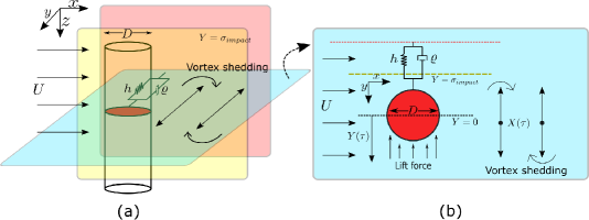
Figure 1: (a) A three-dimensional schematic representation of a cylinder of diameter $D$ with uni-directional motion in the transverse cross-flow direction $y$. A rigid barrier shown in yellow is placed at $Y=\sigma$, obstructing the motion of the cylinder executing VIV. (b) A two-dimensional schematic representation depicting the setup. Lift force being exerted by the fluid on the cylinder in transverse direction to the flow.

$$mY^{\prime\prime} +hY+\varrho Y^{\prime}=S,$$ (1)

$$X^{\prime\prime} +\Omega_{f}^{2}X+\epsilon\Omega_{f}(X^{2}-1)X^{\prime}=F.$$

The prime denotes a derivative with respect to the dimensional time $\tau$. The mass of the oscillator $m$ is composed of the mass of the cylinder $m_{s}$ and the fluid-added mass $m_{f}$ blevins1977flow , defined as $m=m_{s}+m_{f}$. The fluid-added mass is a function of the added mass coefficient $C_{m}$, density of fluid $\rho$ and $D$, defined as $m_{f}=C_{m}\rho D^{2}\pi/4$. The damping coefficient of the oscillator $\varrho$ comprises damping effects due to the structure $r_{s}$ and fluid-added damping $r_{f}$. The fluid-added damping is a function of stall parameter $\gamma$, $\rho$, $D$ and frequency $\Omega$, defined as $r_{f}=\gamma\Omega\rho D^{2}$. In this case, where the structure is undergoing VIV due to cross-flow, $\Omega$ is the frequency of the periodic lift force $\Omega_{f}$. The natural frequency of the structure is defined as $\Omega_{s}^{2}=h/m$ where $h$ is the stiffness of the oscillator. $S$ depicts the lift force acting on the structure due to its interaction with the cross-flow fluid. The nonlinearity of the Van der Pol oscillator is governed by $\epsilon$ and $F$ denotes the effects of the structure’s motion on the wake dynamics. Using the non-dimensional mass ratio $\mu=m/\rho D^{2}$, the Strouhal number $S_{t}=\Omega_{f}D/2\pi U$, the damping ratio $\xi=r_{s}/2m\Omega_{s}$, dimensionless displacement of the structure $y=Y/D$, dimensionless time $t=\Omega_{f}\tau$, and $\delta=\Omega_{s}/\Omega_{f}$, $s=S/m\Omega_{f}D$, $f=F/D\Omega_{f}$, Eq. (1) can be non-dimensionalized as

$$\ddot{y} +\delta^{2}y+(2\xi\delta+\frac{\gamma}{\mu})\dot{y}=s,$$ (2)

$$\ddot{x} +x+\epsilon(x^{2}-1)\dot{x}=f.$$

The overdot denotes derivative with respect to $t$. The wake variable is defined as $x=2C_{L}/C_{Lo}$, where $C_{L}$ and $C_{Lo}$ are the present and reference lift coefficients. $s$ is redefined as $s=Mx$ where $M=C_{Lo}/16\pi^{2}S_{t}^{2}\mu$ is a scaling factor. Effects of structural motion on the wake dynamics are modelled using an acceleration coupling facchinetti2004coupling defined as $f=A\ddot{y}$.

When the structure interacts with a barrier located at $y(t_{-})=\sigma$, it undergoes an instantaneous reversal of velocity at the instant of impact, where $t_{-}$ and $t_{+}$ denote the instants immediately before and after impact, respectively. The instantaneous velocity reversal is defined using a coefficient of restitution $r$; see Eqs. (3) and (4).

$$y(t_{-}) =\sigma,$$ (3)

$$\dot{y}(t_{+}) =-r\dot{y}(t_{-}).$$

and,

$$x(t_{+}) =x(t_{-}),$$ (4)

$$\dot{x}(t_{+}) =\dot{x}(t_{-}).$$

The dynamics is governed by a smooth flow defined using Eqs. (2) and a discrete map at the instant of impact defined by Eqs. (3) and (4). PWS systems exhibiting such behaviour fall under the class of hybrid systems. The section below discusses the effects of an impact on the motion of the structure.

3 Bifurcation analysis

A detailed numerical investigation of Eqs. (2) along with explicit calculations of the non-smooth map that arises from the instantaneous reversal described in Eqs. (3) and (4) is presented here. Numerical integration has been carried out using adaptive time stepping based solver NDSolve in Mathematica. Since small perturbations can lead to diverse outcomes in non-smooth systems, these perturbations must be mapped to ensure that they have reached the barrier in the proper time. This is achieved via the discontinuity mapping. Bifurcation analysis is carried out by varying $U_{r}$ and $\sigma$ as the control parameters. In order to eliminate transience, the first $500$ impacts have been discarded. A Poincaré surface of section $\Sigma$ is defined at $\dot{y}=0$ and the subsequent 200 impacts are observed. If the trajectory interacts with the Poincaré section $N$ times, it is labelled as the period-$N$ or PN orbit.

In Fig. 2, the amplitude response when the barrier is placed at $\sigma_{impact}=-0.150298$ with varying reduced velocity is shown. $\sigma_{impact}$ corresponds to the grazing boundary when $U_{r}=25$. Note that an infinitesimal change in the critical $\sigma$ value may lead to a completely different orbit. Consequently, the value of $\sigma_{impact}$ is considered up to six significant digits. Fig. 2(a) is the bifurcation diagram of structural displacement $y_{0}$ observed stroboscopically for varying reduced velocity ranging between $12\leq U_{r}\leq 25.0$. The figure reveals the existence of period-adding cascades of orbits interspersed with bands of seemingly aperiodic responses. A zoomed section for the range $24.0\leq U_{r}\leq 25.0$ is presented in Fig. 2(b) for clarity. Figs. 2(e) - 2(h) show P2, P3, P4 and P8 orbits for $U_{r}=16$, $19$, $21.5$ and $24.8$ respectively. The red dots highlight Poincaré points on $\Sigma$, which have been plotted in Fig. 2(a) and Fig. 2(b). In Fig. 2(c), simulations from multiple initial states reveal the presence of coexisting P1 and P2 attractors. Although no aperiodic band is observed in this window, such bands appear and get subsequently wider with the addition of periods in the cascade. In Fig 2(d) this aperiodic behaviour, as reflected in phase portrait, is shown for $U_{r}=24.4$.

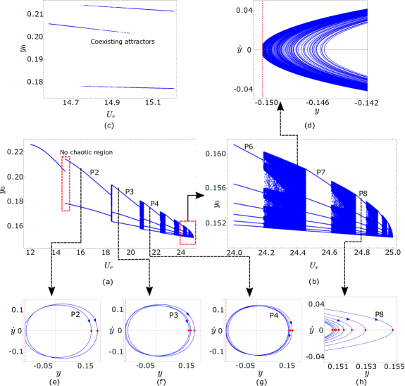
Figure 2: (a) Bifurcation diagram of the structure’s amplitude response $y_{0}$ by varying reduced velocity $U_{r}$ for $r=0.8$ and $\sigma=-0.150298$. (b) Amplitude response $y_{0}$ for $24.0\leq U_{r}\leq 25.0$. (c) Bifurcation diagram depicting the coexistence of P1 and P2 attractors. (d) A typical aperiodic trajectory in phase-space for $U_{r}=24.4$. Periodic orbits: (e) P2 when $U_{r}=16.0$, (f) P3 when $U_{r}=19.0$, (g) P4 when $U_{r}=21.5$, (h) P8 when $U_{r}=24.8$. Dynamics between $500$-$700$ impacts has been presented.

The coexistence of P1 and P2 attractors in Fig. 2(c) is further investigated by varying initial conditions while keeping $U_{r}$ and $\sigma$ fixed at $14.9$ and $-0.150298$, respectively. In Fig. 3, the basins of attraction corresponding to P1 and P2 are shown.

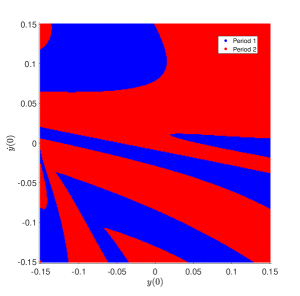
Figure 3: Basins of attraction for $U_{r}=14.9$, $r=0.80$ and $\sigma=-0.150298$.

The placement of barrier at $\sigma_{impact}=-0.150298$ in Figs. 2 and 3 corresponds to the maximum amplitude of oscillations when $U_{r}=25.0$. Thus, a barrier placed there would lead to grazing. A two-parameter bifurcation diagram is shown in Fig. 4. The initial states $y(0)$, $\dot{y}(0)$, $x(0)$ and $\dot{x}(0)$ for these simulations were taken to be $0.0$, $0.0$, $0.0$ and $0.1$ respectively. The dynamics was observed on the Poincaré section $\Sigma$. The results are then color coded according to the periodicity for a given set of chosen parameters (i.e., $\sigma$ and $U_{r}$) post the transient cycles of $500$ impacts. Here, distinct regions of PN, aperiodic and no-impact i.e, P0 responses can be observed.

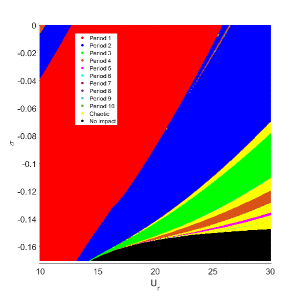
Figure 4: Periodicity in the dynamics of the structure’s motion for $r=0.8$. Periodicity has been calculated after $500$ impacts with a tolerance of $10^{-5}$.

In Fig. 5, barrier distance $\sigma$ is taken as the bifurcation parameter at a constant $U_{r}$ of 25. Fig. 5(b) highlights the bifurcation behaviour when the oscillator is undergoing motion under pure compression i.e., the barrier is placed such that the oscillator cannot reach its equilibrium position. Here, one can observe a period-adding cascade of orbits separated by bands of aperiodic solutions. In Fig. 5(a), the bifurcation behaviour for $\sigma$ near the grazing condition (i.e., $\sigma_{impact})$ for $U_{r}=25.0$ is shown. Higher period orbits are manifested when $\sigma\to\sigma_{impact}$. Fig. 5(g) is a zoomed section of the bifurcation diagram where the amplitude response in the vicinity of P1 and P2 orbits can be observed near $\sigma=-0.020$. A bifurcation branch of a P4 orbit sandwiched between two P2 orbits can be observed here. This bifurcation curve branches out at an acute angle, signifying the occurrence of a non-smooth transition. In Figs. 5(e) and 5(f), the periodic orbits in phase-space corresponding to P2 and P4 for $\sigma=-0.020$ and $\sigma=-0.0210$, respectively, are shown. Similarly, the periodic orbit in phase-space corresponding to a P6 orbit is shown in Fig. 5(c) for $\sigma=-0.149$. An aperiodic orbit in the phase-space, when the barrier is situated at $\sigma=-0.146$, is shown in Fig. 5(d).

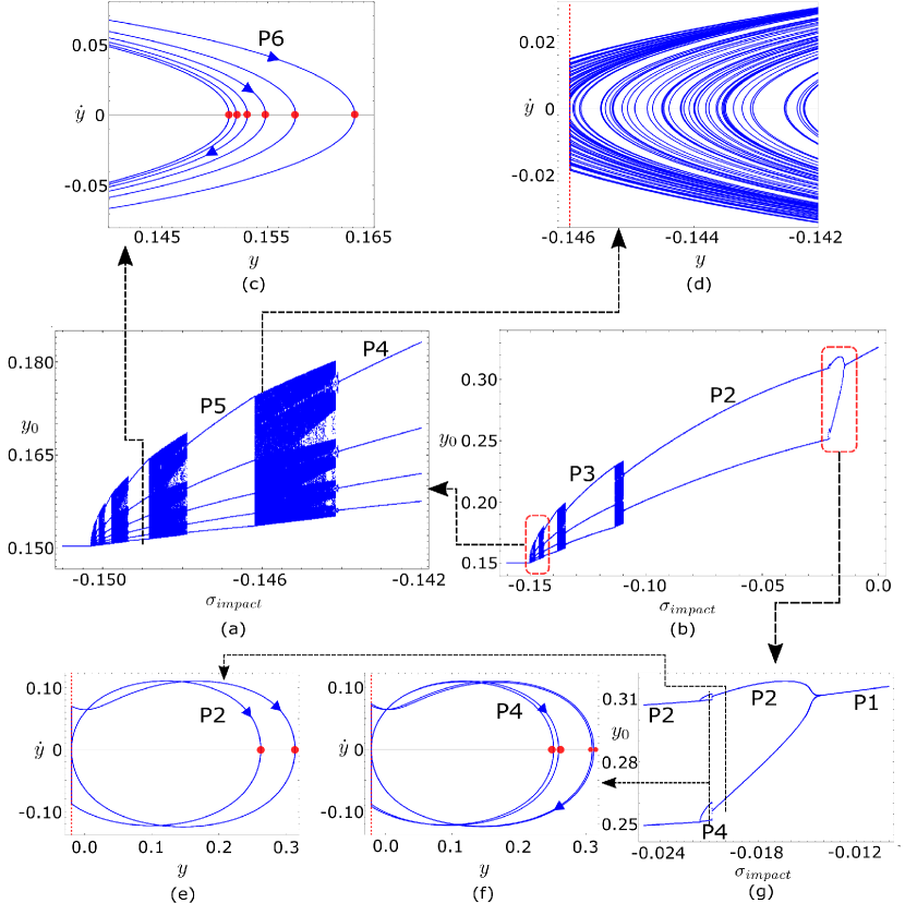
Figure 5: Bifurcation diagram depicting variation in structural amplitude $y_{0}$ as a function of $\sigma$ ranging between (a) $-0.150298\leq\sigma\leq-0.142$ (b) $-0.150298\leq\sigma\leq 0$ for $r=0.8$ and $U_{r}=25.0$. Phase portraits of: (c) P6 orbit when $\sigma=-0.149$, (d) Aperiodic orbit when $\sigma=-0.146$, (e) P2 orbit when $\sigma=-0.020$, (f) P4 orbit when $\sigma=-0.021$. (g) Bifurcation diagram $y_{0}$ when $\sigma$ ranges between $-0.024\leq\sigma\leq-0.010$. Dynamics between $500$-$700$ impacts are considered for these simulations.

The aperiodic behaviour observed between the bifurcation branches of periodic orbits observed in Figs. 2 and 5 is investigated further. To establish that these aperiodic orbits are indeed chaotic, the dynamics on the Poincaré section $\Sigma$, governed by $\dot{y}=0$, is examined. In Fig. 6(a), trajectories intersecting $\Sigma$ for $U_{r}=18.426$ and $18.494$ with a barrier located at $\sigma_{impact}$ and $r=0.8$ are shown. To measure the dimension of the obtained Poincaré section grassberger1983measuring , the correlation dimension $\nu$ has been calculated. This is done by counting the number of points $N(\epsilon_{r})$ enclosed by a small circle of radius $\epsilon_{r}$ and letting the radius grow in size until it encloses the entire attractor. Since the points are clustered in different segments, multiple circles centered at different locations within the attractor are taken and the mean of dimensions at these locations is considered as the entity $C(\epsilon_{r})$ such that $C(\epsilon_{r})=\langle N(\epsilon_{r})\rangle$. The correlation dimension can then be estimated using the expression in Eq. (5)

$$C(\epsilon_{r})\propto\epsilon_{r}^{\nu}.$$ (5)

The number of centres for evaluation of $\nu$ are chosen as multiples of 2 i.e. $2$, $4$, $6\ldots 12$. The values of $\nu$ tends to converge for centres more than $10$. In Fig. 6(a), the mean of $N(\epsilon_{r})$ is estimated by considering $15$ different centres that are circled in the figure. $\epsilon_{r}$ is varied from $0.0001$ to $0.06$ in steps of $10^{-4}$ to cover the entire finger-shaped attractor. The correlation dimension $\nu$ is then estimated from the slope of the log-log plot between $\epsilon_{r}$ and $C(\epsilon_{r})$. A linear fit corresponding to obtained graph is presented Fig. 6(b). Here, $\nu$ is estimated to be $2.4$. Since $\nu$ is an non-integer value, the corresponding dynamics observed on the Poincaré section possess a fractal like structure, and hence, can be characterized as a strange attractor, indicative of the chaotic behaviour. In Fig. 6(c) Poincaré sections are shown for various reduced velocities and barrier at $\sigma_{impact}$. The corresponding correlation dimensions obtained have non-integer values as well. In Fig. 6(d) $\Sigma$ corresponding to varying barrier distances with reduced velocity kept fixed at $U_{r}=25.0$ have been presented. The values of $U_{r}$ and $\sigma$ chosen here correspond to the aperiodic regions in the bifurcation diagrams that separate the periodic orbits i.e., between P2-P3, P3-P4 and P5-P6 orbits. For each of these Poincaré sections, the correlation dimensions obtained are non-integer values, thus verifying the existence of fractal-like strange attractors sandwiched between periodic solutions.

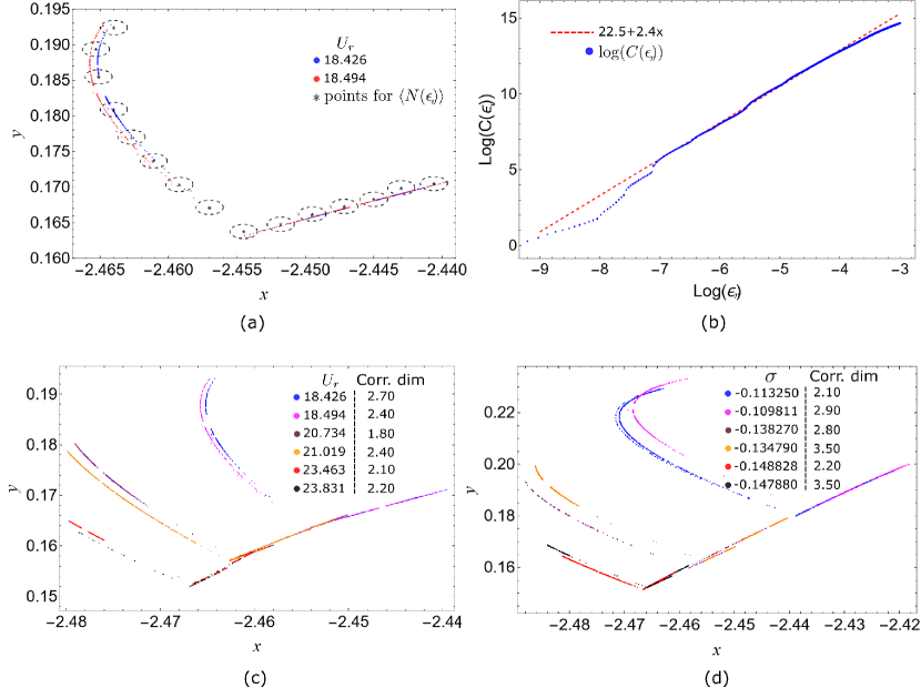
Figure 6: (a) Poincare section $\dot{y}=0$ for $U_{r}=18.426$ and $18.494$. $N(\epsilon_{r})$ is counted from the centre of circles shown; $C(\epsilon_{r})$ defined as $\langle N(\epsilon_{r})\rangle$. (b) Correlation dimension estimation from slope of $\log(C(\epsilon_{r}))$ vs $\log(\epsilon_{r})$. Poincare section $\dot{y}=0$ for (c) varying velocity $U_{r}$ and barrier kept fixed at $\sigma=-0.150298$; (d) varying barrier distance $\sigma$ with velocity fixed at $Ur=25.0$.

The effect on the dynamics due to the variation of coefficient of restitution $r$ is investigated next. In Fig. 7, the variation in amplitude response is shown against coefficient of restitution $r$, when the barrier is fixed at $\sigma=-0.021$ and reduced velocity fixed at $U_{r}=25.0$. The red dots shown in Figs. 5(f) and 7 correspond to the Poincaré points of a P4 orbit, when $U_{r}=25.0$, $\sigma=-0.021$ and $r=0.8$. The observed behaviour is similar to Fig. 5(g), where a P4 orbit is sandwiched between two P2 orbits. In Fig 8, a two-parameter bifurcation diagram is presented. Here, periodicity in dynamics is observed to follow a distinct adding pattern, separated by chaotic bands. The reduced velocity for these simulations is kept fixed at $U_{r}=25.0$. The first $500$ impacts have been discarded to eliminate transient effects and recurrence in a trajectory at the same point in the state space is considered when the Euclidean distance at the point of interest is close to the reference point within a tolerance of $10^{-5}$. This is done to compute the periodicity of the orbits. In the observed period-adding cascade, higher period orbits tend to appear in the vicinity of the grazing region that corresponds to $\sigma=-0.150298$ for $U_{r}=25.0$. A narrow region of P4 orbit is observed between two P2 regions; see Fig. 8. Using $U_{r}$ as one of the bifurcation parameters, similar behaviour is observed. The stable behaviour here is examined by keeping the barrier fixed while varying the reduced velocity and coefficient of restitution. This is shown in Fig. 9. The barrier is kept fixed at $\sigma=-0.0210$, away from the grazing condition for $U_{r}=25.0$. This distance corresponds to a value where P4 orbit was observed in Fig. 8 with $r=0.8$ and $U_{r}=25.0$.

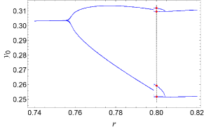
Figure 7: Bifurcation in amplitude of the structure for various values of coefficient of restitution. Here, reduced velocity fixed at $U_{r}=25.0$ and with a barrier placed at $\sigma=-0.021$. The red dots correspond to Poincaré points for P4 shown in Fig. 5(g).

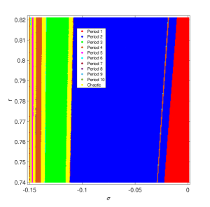
Figure 8: Two-parameter bifurcation diagram plotted between $\sigma$ and $r$ for reduced velocity $U_{r}=25.0$.

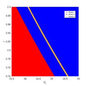
Figure 9: Two-parameter bifurcation diagram between $U_{r}$ and $r$ plotted for $\sigma=-0.0210$.

For the above simulations, the coupling and the wake parameters, $A$ and $\epsilon$, are taken as $12$ and $0.3$, respectively, such that $A/\epsilon=40$. This ensures that the dynamical model is compatible with experimental observations in facchinetti2004coupling . The parameter $A$ determines the strength of coupling between the structure and associated wake dynamics, while $\epsilon$ controls the strength of non-linearity of the wake oscillator. In Fig. 10(a), the variation in amplitude response of the structure as a function of reduced velocity in the absence of a barrier is presented. The values of $A$ and $\epsilon$ are varied while ensuring that the ratio $A/\epsilon=40$ is constant. It is observed that the amplitude of vibrations of the structure increases as the coupling parameter $A$ increases. In Fig. 10(b), the amplitude response is shown in the absence of a barrier where $A$ kept fixed at $A=10$ and the ratio $A/\epsilon$ is varied. The ratio is kept close to 40 to ensure that observed dynamics correspond to the original physical system; see the models discussed by Facchinetti et. al bishop1964lift ; facchinetti2004coupling . In this case, the amplitude response increases as the ratio $A/\epsilon$ is increased. The location of the rigid barrier is chosen such that, in the parameter regime of interest, the structure grazes the barrier for only one parameter. This implies that the vibration amplitude of the structure is the lowest in the domain of interest, ensuring that all other values of $A$ and $\epsilon$ will undergo an impact with the rigid barrier transversally. This is further demonstrated graphically. In Fig. 10(c), the trajectories depicting the structure’s oscillations are presented. The observations are made when the vibrations have attained a steady state for barrier placed at $\sigma=-0.13181$. The barrier, shown as an orange dashed line, corresponds to the grazing condition for $A=10$ and $\epsilon=0.25$ such that $A/\epsilon=40$. The black curve in Fig. 10(c) grazes the barrier, while the blue and red curves interact with the barrier transversally. Similarly, in Fig. 10(d), the structur oscillations are shown when the barrier is located at $\sigma=-0.130979$, corresponding to the grazing condition for $A=10$, and $\epsilon=0.333$, such that $A/\epsilon=30$. Thus, the black curve with $A/\epsilon=30$ grazes the barrier while the blue and red curves corresponding to $A/\epsilon=50$ and $40$, respectively, impact the barrier transversally. A bifurcation analysis is subsequently carried out.

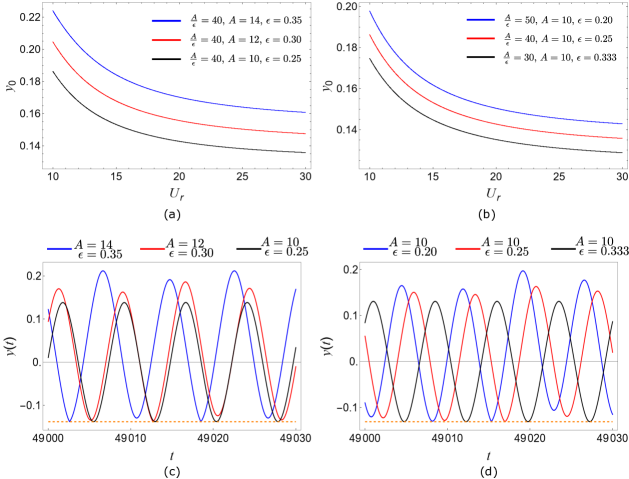
Figure 10: Amplitude response without barrier for (a) $A=14$, $12$ and $10$ such that $A/\epsilon=40$, (b) $A/\epsilon=50$, $40$ and $30$. Structural displacement with barrier placed at (c) $\sigma=-0.13181$ by varying $A=14$, $12$ and, $10$ ensuring $A/\epsilon=40$. (d) $\sigma=-0.130979$ for $A/\epsilon=50$, $40$ and $30$.

Figs. 11(a), (c) and (e) depict the dynamical change in the amplitude response of the structure as a function of reduced velocity. The initial $500$ impacts are discarded to remove any transient effects and the ratio in all the cases is $A/\epsilon=40$. The discontinuity boundary kept fixed at $\sigma=-0.13181$, which corresponds to the grazing condition for $A=10$, $\epsilon=0.25$ and $U_{r}=25.0$. For $12\leq U_{r}\leq 25.0$, only P1 and P2 orbits can be observed for $A=14$ and $\epsilon=0.35$; see Fig. 11(a). As the coupling parameter $A$ reduces, the maximum amplitude of vibration of the structure reduces, thus leading to non-transversal interactions of trajectories with the boundary. As the value of $A$ approaches $10$ for which $\sigma$ is near grazing value of $-0.13181$, higher period orbits separated by chaotic bands are observed; see Figs. 11(c) and (e). When $A=10$ and $\epsilon=0.25$ in Fig. 11(e), existence of higher periodic orbits is observed in the vicinity of $U_{r}=25.0$ beyond which no impact with the barrier occurs. Similarly, in Figs. 11(b), (d) and (f), the amplitude response of the cylindrical structure is shown for $A/\epsilon=50$, $40$ and $30$ ensuring $A=10$. The barrier is situated at $\sigma=-0.130979$, corresponding to the grazing condition for $A=10$, $\epsilon=0.333$ and $U_{r}=25.0$. Again a similar phenomenon is observed. With $A=10$ and decreasing $A/\epsilon$, the amplitude of oscillations of the structure decreases and the cylinder interacts with the barrier more non-transversally. A cascade of periodic orbits separated by chaotic behaviour is observed. As $A$, $\epsilon$ and $U_{r}$ approach the grazing condition of $\sigma=-0.130979$, higher periodic orbits are observed with bands of chaotic solutions; see Fig. 11(f). However, in all of these results, no chaotic solutions are observed between P1 and P2 orbits.

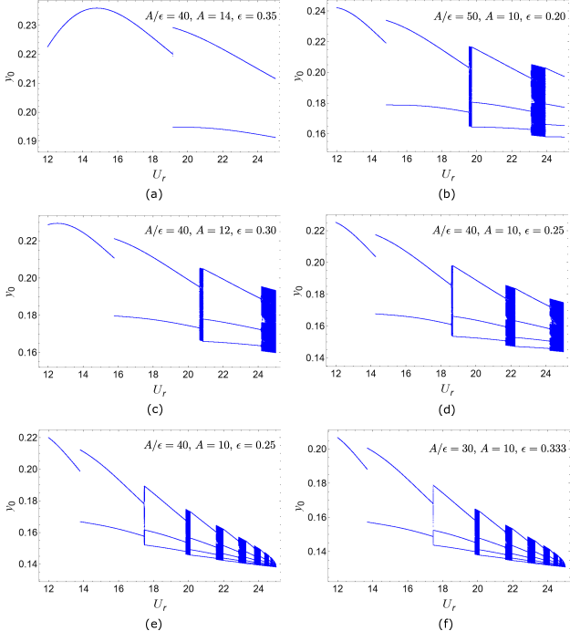
Figure 11: Bifurcation diagram with barrier placed at $\sigma=-0.13181$ for (a) $A=14$ (c) $A=12$ (e) $A=10$ ensuring $A/\epsilon=40$. Bifurcation diagram with barrier placed at $\sigma=-0.130979$ and $A=10$ such that (b) $A/\epsilon=50$, (d) $A/\epsilon=40$ (f) $A/\epsilon=30$.

The following section presents stability analysis of this non-smooth system using Floquet theory. Here, the methods and numerical algorithms are presented and inferences about the dynamical behaviour are drawn by correlating the results with the bifurcation studies presented above.

4 Stability analysis

Bifurcation diagrams presented above indicate that as parameters like $U_{r}$ or $\sigma$ is varied, existing orbits become unstable, resulting in newer periodic or aperiodic orbits. Hence, it is essential to carry out a stability analysis to investigate when an orbit might become unstable, therefore revealing routes to chaos. This sections considers two methods of investigating the stability of a limit cycle - an eigenvalue analysis of the fundamental solution matrix of the orbit under consideration followed by evaluation of Lyapunov exponents.

4.1 Floquet multipliers

The stability of orbits obtained for various parameters of the FSI system undergoing impacts i.e., Eq. (3) and Eq. (4) is investigated next. Since the system under consideration is piece-wise smooth and leads to orbiting steady states, a combination of Floquet theory along-with the consideration of discontinuity mappings are taken into consideration while performing the stability analyses. For smooth systems, Floquet multipliers are the eigenvalues of the global state transition matrix (STM) for any given periodic orbit. However, in hybrid dynamical systems, there are discontinuous transitions in the phase-space at the instant of an impact. The Floquet multipliers jump at the instant of impact. Hence, the global STM or the monodromy matrix is composed of local STMs and STMs at the instant of impact, also known as the saltation matrices. These matrices are multiplied in the order of occurrence of dynamical evolution. The state transition of any perturbed trajectory at the instant of an interaction with the barrier is defined by a transverse discontinuity map (TDM). The approach for obtaining the complete monodromy matrix and the role of appropriately defining the TDM is presented next. In Fig. 12, the phase portrait of a P2 orbit of a hybrid system undergoing impact twice with a discontinuity boundary $\Sigma_{2}$, depicted by a black dashed line, is shown. The monodromy matrix $\Phi(T)$ for this orbit of period $T$ (time after which the orbit repeats itself) comprises products of several STMs applied in the correct order of events. Here, the orbit is initiated on the section $\Sigma_{1}$ and it traverses to the switching surface $\Sigma_{2}$ by state transition $\Phi_{1}$. The state gets mapped by another transition matrix $S_{1}$ to a new state. The mapping of this state back to $\Sigma_{2}$ again is given by $\Phi_{2}$. It undergoes a state transition $S_{2}$ and $\Phi_{3}$ subsequently to land up at $\Sigma_{1}$ and the orbit repeats itself. Thus, over one cycle, the state transition matrix can be defined as

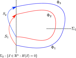
Figure 12: The schematic of a P$2$ limit cycle undergoing two instances of instantaneous reversals at the instants of impact with $\Sigma_{2}$, depicted as black dashed line. The red solid line corresponds to flow governed by the STM $\Phi_{2}$, the red dashed line corresponds to state transition at the instant of first impact (using saltation matrix $S_{1}$), the blue solid line corresponds to flow governed by STM $\Phi_{1}$, the blue dashed line corresponds to state transition at the instant of second impact (using saltation matrix $S_{2}$).

$$\Phi(T)=\Phi_{3}\cdot S_{2}\cdot\Phi_{2}\cdot S_{1}\cdot\Phi_{1},$$ (6)

where $S_{i}$ is the STM or saltation matrix at the instant of $i^{th}$ impact. Similarly for a given solution obtained numerically with period $T$ and $n$ number of impacts, the monodromy matrix is defined by Eq. (7).

$$\Phi(T)=\Phi_{n}\prod_{i=1}^{n-1}S_{i}\cdot\Phi_{i}.$$ (7)

According to the Floquet theory, the monodromy matrix is evaluated by integrating the fundamental solution matrix over one complete orbit. This ensures that the time varying Jacobian over the limit cycle is now observed over one period, making the entries of the state transition matrix constant. Here, the saltation matrix describes the mapping of orbits in the local neighbourhood at the instants when the dynamical system undergoes an impact with a discontinuity boundary. Consider an arbitrary dynamical system $\mathbf{x}$ with a small perturbation $\mathbf{y}$. The governing dynamics and its corresponding variational equations are presented in Eq. (8).

$$\dot{\mathbf{x}} =\mathbf{F}(\mathbf{x}),$$ (8)

$$\dot{\mathbf{y}} =\mathbf{\nabla}\mathbf{F}(\mathbf{x})^{T}\cdot\mathbf{y}.$$

Fig. 13 is a schematic representation of two perturbed trajectories obeying Eq. (8). The periodic trajectory of the primary system starts initially from $\mathbf{x}_{p}$ and undergoes impact at $H(\mathbf{x}_{i})=0$. Here, $H(\mathbf{x})=0$ is a scalar function that models the discontinuity boundary.

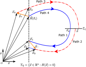
Figure 13: A schematic of the phase portrait of two nearby trajectories exhibiting impact at $\Sigma_{2}$. The blue line shows the actual trajectory. The red dashed line denotes the perturbed trajectory. This is a representative figure and is not to scale. The black dashed line $\Sigma_{1}$ denotes the Poincaré section from which both the trajectories are initiated and $\Sigma_{2}$ denotes the discontinuity boundary. The amber line denotes the perturbation vector $y$.

However, any perturbed trajectory from this periodic orbit will not undergo an impact at the same instant when the primary orbit impacts the discontinuity boundary. Therefore, there exists a time difference between impacts for any two trajectories of a given hybrid system. To ensure that the perturbed trajectory is appropriately mapped at its instant of impact, a mapping of the perturbed trajectory at the instant of impact i.e., $\mathbf{y}_{-}$ to $\mathbf{y}_{+}$ is performed. This mapping ensures that the perturbed trajectory will reach the discontinuity boundary after the time difference between the impact of the two trajectories has elapsed. The perturbed trajectory starts from $\mathbf{\hat{x}}=\mathbf{x}_{p}+\mathbf{y}_{0}$ and at the instant of impact of the primary trajectory (when $\mathbf{x}_{0}=\mathbf{x}_{i}+\mathbf{y}_{-}$) gets mapped from $\mathbf{y}_{-}$ to $\mathbf{y}_{+}$ such that $\mathbf{x}_{4}=\mathbf{R}(\mathbf{x}_{i})+\mathbf{y}_{+}$. Here, $\mathbf{R}(\mathbf{x}_{i})$ represents the mapping of the primary periodic orbit (i.e., the impact of the structure with the barrier). The trajectory evolves from $\mathbf{x}_{4}$ and reaches $\mathbf{x}_{3}$ lying on the discontinuity boundary within the time difference as previously mentioned. This evolution can be interpreted as the perturbed trajectory $\mathbf{x}_{0}=\mathbf{x}_{i}+\mathbf{y}_{-}$ undergoing impact at $H(\mathbf{x}_{2})=0$ after the time difference and getting mapped to $\mathbf{x}_{3}=\mathbf{R}(\mathbf{x}_{2})$. The above mapping of the perturbed trajectory is analytically modeled via a state transition matrix, also known as saltation matrix in literature chawla2022stability ; see Eq. (9).

$$\mathbf{y}_{+}=S\cdot{\mathbf{y}_{-}}.$$ (9)

The saltation matrix obtained by retaining only the first order terms of the Taylor series is presented in Eq. (10).

$$S= \mathbf{\nabla}\mathbf{R}(\mathbf{x}_{i})^{T}$$ (10)

$$+\frac{\Big{(}\mathbf{F}(\mathbf{R}(\mathbf{x}_{i}))-\mathbf{\nabla}\mathbf{R}(\mathbf{x}_{i})^{T}\cdot\mathbf{F}(\mathbf{x}_{i})\Big{)}}{\mathbf{\nabla}H(\mathbf{x}_{i})^{T}\cdot\mathbf{F}(\mathbf{x}_{i})}\mathbf{\nabla}H(\mathbf{x}_{i})^{T}$$

where $\mathbf{x}_{i}$ represents the state of the dynamical system at the instant of impact, $\mathbf{R}(\mathbf{x}_{i})$ is the reset map at the instant of impact, $\mathbf{F}(\mathbf{x})$ denotes the underlying vector field and $H(\mathbf{x})=0$ represents the discontinuity boundary where an impact or reset occurs.

For the given FSI system described by Eq (3) along-with Eq (4), the state space is 4 dimensional i.e., $\mathbf{x}=[y\ \dot{y}\ x\ \dot{x}]$ and the dynamics evolves according to the vector field $\mathbf{F}(\mathbf{x})$ described by Eq. (11).

$$\mathbf{F}=\begin{bmatrix}\dot{y}\\ -\delta^{2}y-\alpha\dot{y}+Mx\\ \dot{q}\\ -x-\epsilon(x^{2}-1)\dot{x}+A(-\delta^{2}y-\alpha\dot{y}+Mx)\\ \end{bmatrix},$$ (11)

where $\alpha=(2\xi\delta+\gamma/\mu)$. The discontinuity barrier is defined using a scalar function $H(\mathbf{x})=0$ where $H(\mathbf{x})=y-\sigma$. At the instant of impact a reset map $\mathbf{R}(\mathbf{x})$ is initiated such that $\mathbf{R}(\mathbf{x})=[y\ -r\dot{y}\ x\ \dot{x}]$; $r$ being the coefficient of restitution defined previously in Eq. (4). The analytical form of the saltation matrix given by Eq. (10) is represented in Eq. (12),

$$S=\begin{bmatrix}-r&0&0&0\\ \frac{(1+r)}{\dot{y}}(-\delta^{2}y+Mx)&-r&0&0\\ 0&0&1&0\\ A\alpha(1+r)&0&0&1\end{bmatrix}.$$ (12)

The fundamental solution matrix $\mathbf{Y}(t)$ is numerically evaluated by considering an orthogonal set of perturbed vectors such that $\mathbf{Y}(0)=\textit{I}_{n\times n}$. Each perturbed vector is a column entry of $\mathbf{Y}$ and evolves using Eq. (8). Next, the periodicity of the FSI system is obtained numerically after discarding $500$ impacts with the barrier to eliminate any transient effects. The monodromy matrix and its eigenvalues are evaluated after one time period from Eq. (7). The numerical procedure has been outlined in Algorithm 1 below.

Algorithm 1 Floquet multipliers from monodromy matrix $\mathbf{\phi}$

1. Initialize: $\mathbf{x}(0)$, ensure $H(\mathbf{x})>0$

2. Initialize $U_{r}$ $\ignorespaces\triangleright$ Bifurcation parameter

3. Initialize: $\mathbf{\Phi}=\textit{I}_{n\times n}$, count $=0$

4. Initialize: $n_{max}$ $\ignorespaces\triangleright$ Maximum allowable impacts

while count $\leq$ $n_{max}$ do

     Integrate: $\dot{\mathbf{x}}=\mathbf{F}(\mathbf{x})$

     if $H(\mathbf{x})=0$ then $\ignorespaces\triangleright$ Occurrence of impact

         Reset Map: $\mathbf{x}\leftarrow\mathbf{R}(\mathbf{x})$

     end if

     if $\dot{x}=0$ $\&\&$ count $\geq n_{max}/2$ then

         Store $\mathbf{x}$, $t$ for evaluation of time period $T$

         $T=\{t\in\mathbb{R}^{1}:\mathbf{x}(t+\tilde{n}T)=\mathbf{x}(t),\tilde{n}\in\mathbb{I}\}$

     end if

     if count $=$ $n_{max}$ then $\ignorespaces\triangleright$ Remove transients

         Store: $\mathbf{x}_{init}$ $\leftarrow\mathbf{x}(t)$ and $t_{init}\leftarrow t$

     end if

end while

Initialize: $\mathbf{x}\leftarrow\mathbf{x}_{init}$ at $t_{init}$ $\ignorespaces\triangleright$ Begin at steady state

Initialize: $\mathbf{Y}(0)=\textit{I}_{n\times n}$ $\ignorespaces\triangleright$ Evaluation of $\mathbf{\Phi}_{i}$

while $t_{init}\leq t\leq(t_{init}+T)$ do $\ignorespaces\triangleright$ Integrate over period $T$

     Integrate: $\dot{\mathbf{x}}=\mathbf{F}(\mathbf{x})$

     Integrate: $\dot{\mathbf{Y}}=(\nabla\mathbf{F})^{T}\cdot\mathbf{Y}$

     if $H(\mathbf{x})=0$ then $\ignorespaces\triangleright$ Occurrence of impact

         $\mathbf{\Phi}_{i}\leftarrow\mathbf{Y}$

         $\mathbf{\Phi}\leftarrow\mathbf{\Phi}_{i}\cdot\mathbf{\Phi}$

         Evaluate $\mathbf{S}$ from Eq. (12) $\ignorespaces\triangleright$ saltation matrix

         $\mathbf{\Phi}\leftarrow\mathbf{S}\cdot\mathbf{\Phi}$

         Reset Map: $\mathbf{x}\leftarrow\mathbf{R}(\mathbf{x})$

         Reinitialize: $\mathbf{Y}\leftarrow\textit{I}_{n\times n}$

     end if

end while

5. $\mathbf{\Phi}\leftarrow\mathbf{Y}\cdot\mathbf{\Phi}$ $\ignorespaces\triangleright$ Evaluate monodromy matrix

6. Evaluate eigenvalues of $\mathbf{\Phi}$ to get Floquet multipliers

In Fig. 14, the Floquet multipliers $\rho_{i}$ of the monodromy matrix have been shown as the reduced velocity $U_{r}$ is varied. A one to one correspondence is drawn with the dynamics observed on the bifurcation diagram. A barrier is placed at $\sigma_{impact}$ (grazing condition for $U_{r}=25.0$) with $r=0.8$. The region ranging between $-1\leq\rho_{i}\leq 1$ corresponds to a stable periodic orbit. The dashed vertical lines highlight the observed bands of chaotic orbits. Floquet multipliers are within the unit circle for stable orbits. As $U_{r}$ is varied, the Floquet multiplier approaches $-1$, eventually resulting in a bifurcation to chaotic orbits at $\rho_{i}=-1$. Additionally, in the parameter region where a transition from P1 to P2 orbit is observed, the Floquet multipliers discontinuously jumps to a value with norm less than unity. This suggests a birth of a new stable periodic orbit. Eventually, the absolute value of the Floquet multipliers decreases to $-1$ before it approaches the next instant of a non-smooth bifurcation. Similarly, in Fig. 15, the Floquet multipliers are shown as the barrier distance is varied, while the reduced velocity is kept fixed at $U_{r}=25.0$ and $r=0.8$. Similar transitions in values of the Floquet multipliers are observed near bifurcation occurrences. This is clearly reflected in the bifurcation diagram as well.

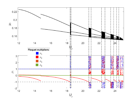
Figure 14: Floquet multipliers vs reduced velocity $U_{r}$ for barrier placed at $\sigma=-0.150298$ and $r=0.8$.

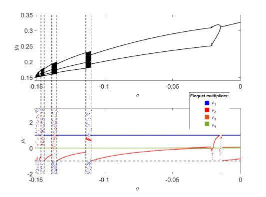
Figure 15: Floquet multipliers vs barrier distance $\sigma$ when reduced velocity is $U_{r}=25.0$ and $r=0.8$.

Moreover, it was also observed that one of the Floquet multiplier is always unity i.e. it lies on the unit circle. For an autonomous dynamical system, this implies that there is an eigendirection along that which there is no variation in the magnitude of perturbation i.e. the primary and the perturbed trajectory neither converge nor diverge from each other nayfeh2008applied . This also verifies that the TDM that correctly maps the perturbed trajectories at the instant of impact and the results verify the established Floquet theory. It is to be noted here that Floquet theory is not directly applicable for aperiodic oscillatory responses. This is because, the trajectories do not recur and thus, the product of matrix multiplications blow up. This reflects in Fig. 14(b) as noisy bands of $\rho_{i}$ with magnitude greater than unity. An alternate marker of chaotic dynamics is the presence of positive Lyapunov exponents. Lyapunov spectra is thus obtained below to analyze the observed aperiodic phenomena in this non-smooth system.

4.2 Lyapunov exponents

In this section, the stability of orbits is investigated by estimating the rate of exponential divergence of their nearby perturbed trajectories. The rates of exponential divergence or the Lyapunov exponents are computed as follows. Starting from a periodic orbit $\mathbf{x}_{0}$, an orthogonal set of perturbed trajectories are initialized. The initial magnitude of the perturbed trajectories is set to a small value of $r_{0}=0.0001$ units. This implies that the perturbed vectors lie on a hypersphere of radius $r_{0}$. Then, this hypersphere is allowed to evolve for the $n^{th}$ time from $t$ to $t+t_{0}$ after which, the growth rate $r_{n}$ of all the perturbed trajectories is noted. The perturbed trajectories evolve according to the variational formalism of the dynamical system under investigation (see Eq. (8)). Each time the primary system undergoes an impact with the discontinuity boundary, the perturbed trajectory gets mapped by Eq. (9) in phase-space using the saltation matrix in Eq. (12). After a time interval of $t_{0}$, the initialized hypersphere has now evolved into a hyper-ellipsoid. The average largest Lyapunov exponent $\lambda_{1}$ is measured from the growth rate of the perturbations along the major axis of the hyper-ellipsoid using Eq. (13),

$$\lambda_{i}=\frac{1}{t_{0}N}\Sigma_{n=1}^{N}\ln\frac{r_{n}}{r_{0}}.$$ (13)

At this instant, the set of perturbed vectors is once again orthogonalized using the Gram-Schmidt process with respect to one of the perturbed vectors (along eigenvector with the largest Lyapunov exponent), meanwhile ensuring the magnitude is again scaled down to $r_{0}$. This is achieved by performing a QR decomposition (QRD) followed by scaling of the vectors by $r_{0}$. Thus, once again an initial hypersphere of radius $r_{0}$ is obtained but the vectors now are oriented differently. This process is repeated and the growth rate is monitored and reset stroboscopically i.e. when $t\%t_{0}=0$. This step is followed by a QRD. This procedure has been described in Algorithm 2. The Lyapunov exponents along each orthogonal direction are thus obtained by evaluating steps 6-8 in Algorithm 2; also see Eq. (13).

Algorithm 2 Lyapunov exponent for hybrid systems using $\mathcal{O}(1)$ TDM

1. Initialize: $\mathbf{x}(0)$ , ensure $H(\mathbf{x}\geq 0)$

2. Initialize: $U_{r}$ $\ignorespaces\triangleright$ Bifurcation parameter

3. Initialize: $\mathbf{y}_{i}(0)$ for $i\leq n$ using QRD

4. Rescale: $\mathbf{y}_{i}(0)\leftarrow r_{0}*\mathbf{y}_{i}(0)$

5. Initialize: $n_{max}$ $\ignorespaces\triangleright$ Maximum allowable impacts

while count $\leq n_{max}$ do

     Integrate: $\dot{\mathbf{x}}=\mathbf{F}(\mathbf{x})$

     if $H(\mathbf{x})=0$ then $\ignorespaces\triangleright$ Occurrence of impact

         Evaluate: $\mathbf{R}(\mathbf{x})$ and $\mathbf{y}_{+}$

         Reset Map: $\mathbf{x}\leftarrow\mathbf{R}(\mathbf{x})$

         Reinitialize: $\mathbf{y}_{i}\leftarrow\mathbf{y}_{i,+}=S\cdot\mathbf{y}_{i,-}$ $\ignorespaces\triangleright$ TDM using saltation matrix

     end if

     if $\big{(}t\%t_{0}\big{)}=0$ then

         

         if count $\geq n_{max}/2$ then

              Store: $r_{i}\leftarrow\frac{1}{r_{0}}\|\mathbf{y}_{i}\|$

         end if

         Reinitialize: $\mathbf{y}_{i}\leftarrow r_{0}*\text{QRD of }\mathbf{y}_{i}$

     end if

end while

6: Evaluate: $\ln r_{i}$ $\ignorespaces\triangleright$ Store all $\ln r_{i}$

7: LE${}_{i}\leftarrow\frac{1}{t_{0}N}\Sigma_{n=1}^{N}\ln\frac{r_{n}}{r_{0}}$ $\ignorespaces\triangleright$ LEs measured N times

8: $\lambda_{i}\leftarrow\langle\text{LE}_{i}\rangle$ $\ignorespaces\triangleright$ Mean of all LEs

In Fig. 16, the variation of the largest Lyapunov exponent (LLE) as a function of reduced velocity as well as the corresponding bifurcation diagrams are shown. The barrier is kept fixed at $\sigma_{impact}$ and $r=0.8$. The LLE has been computed stroboscopically at $t_{0}=\pi$ in algorithm 2 for $800$ impacts with the barrier. The LLE is a measure of the maximum rate of exponential divergence between two nearby perturbed trajectories. Positive values of LLE in Fig. 16 correspond to trajectories that diverge from each other; indicating the occurrence of chaos. This can also be verified from the corresponding bifurcation diagram. The dashed lines in the figure highlight the intervals within which chaotic orbits are observed. These regions also show a positive value of the LLE. Similarly, in Fig. 17, LLEs have been shown as the barrier distance is varied, ranging between $-0.150298\leq\sigma\leq 0$. The flow velocity here is kept fixed at $U_{r}=25.0$ and $r=0.8$. The LLE is zero for all periodic orbits and suddenly jumps to positive values where chaotic orbits are observed in the corresponding amplitude response diagram.

Therefore, the TDM, using the derived saltation matrix, accurately determines the dynamical stability of the FSI system undergoing impacts. The algorithms presented above can also be adapted to consider higher order estimations of the TDM for better estimation of the states near an impact chawla2022stability . Furthermore, the proposed algorithms can be used to study non-smooth dynamical systems of different formalisms i.e., the Filippov and piecewise continuous kind and can be extended to higher dimensions. The findings from the presented work are summarized in the section below.

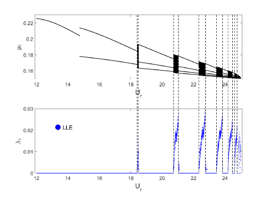
Figure 16: Largest lyapunov exponent vs reduced velocity $U_{r}$ when barrier is placed at $\sigma=-0.150298$ and $r=0.8$.

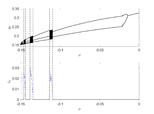
Figure 17: Largest lyapunov exponent vs barrier distance $\sigma$ when reduced velocity is $U_{r}=25.0$ and $r=0.8$.

5 Conclusions

The effect of non-smooth impacts with a rigid barrier on the VIV characteristics of a sdof cylindrical system is investigated in this paper. A detailed study of the underlying dynamical bifurcations, followed by the stability analysis of the concerned FSI system undergoing vibro-impacts, is presented. Non-smooth dynamical phenomena like period adding, periodic bifurcation branches separated by chaotic orbits, and finger-shaped chaotic attractors are observed. Moreover, there is the coexistence of P1 and P2 stable attractors with intertwined basins of attraction. By varying the coupling strength and non-linearity of the wake oscillator, cascades of higher periodic orbits were observed in the vicinity of the grazing condition.

Furthermore, algorithms for obtaining Floquet multipliers and Lyapunov spectra for non-smooth dynamical systems are proposed and demonstrated for the vibro-impact system under fluid flow. To capture the discontinuous jump of the orbits in phase-space in the presence of a non-smooth barrier, a discontinuity map was numerically estimated at the instant of impact. Results indicate that one of the Floquet multipliers approaches and exits the unit circle as the system loses stability. At this instant, the bifurcation diagrams showed the presence of large-amplitude chaotic oscillations. This was further backed up by a positive Lyapunov exponent obtained by incorporating the TDM at impacts. Additionally, jumps in the Floquet multipliers indicate the occurrence of a non-smooth bifurcation. The jumps occurred when one of the orbits lost stability, and another came into existence upon variation of a system parameter; here, the barrier distance and reduced flow velocity. The Floquet spectra and the largest Lyapunov exponents, obtained by using variational formalism and incorporating non-smooth saltation terms, are in good agreement with the numerically obtained bifurcation diagrams.

Declarations

The authors acknowledge the support of Science Foundation Ireland NexSys Project 21/SPP/3756, Enterprise Ireland SEMPRE Project and Sustainable Energy Authority of Ireland TwinFarm project RDD/604.

Conflict of interest

The authors declare that they have no conflict of interest.

Availability of data

Not applicable.

Availability of code

All codes implemented in this paper is available upon request from the corresponding author.

References

- \bibcommenthead
- (1) Williamson, C.H., Govardhan, R.: Vortex-induced vibrations. Annual Review of Fluid Mechanics 36, 413–455 (2004)
- (2) Williamson, C., Govardhan, R.: A brief review of recent results in vortex-induced vibrations. Journal of Wind engineering and industrial Aerodynamics 96(6-7), 713–735 (2008)
- (3) Facchinetti, M.L., De Langre, E., Biolley, F.: Coupling of structure and wake oscillators in vortex-induced vibrations. Journal of Fluids and structures 19(2), 123–140 (2004)
- (4) Newman, D.J., Karniadakis, G.E.: A direct numerical simulation study of flow past a freely vibrating cable. Journal of Fluid Mechanics 344, 95–136 (1997)
- (5) Sarpkaya, T.: A critical review of the intrinsic nature of vortex-induced vibrations. Journal of fluids and structures 19(4), 389–447 (2004)
- (6) Gabbai, R.D., Benaroya, H.: An overview of modeling and experiments of vortex-induced vibration of circular cylinders. Journal of sound and vibration 282(3-5), 575–616 (2005)
- (7) Bishop, R.E.D., Hassan, A.: The lift and drag forces on a circular cylinder oscillating in a flowing fluid. Proceedings of the Royal Society of London. Series A. Mathematical and Physical Sciences 277(1368), 51–75 (1964)
- (8) Balasubramanian, S., Skop, R.: A nonlinear oscillator model for vortex shedding from cylinders and cones in uniform and shear flows. Journal of Fluids and Structures 10(3), 197–214 (1996)
- (9) Skop, R.A., Balasubramanian, S.: A new twist on an old model for vortex-excited vibrations. Journal of Fluids and Structures 11(4), 395–412 (1997)
- (10) Hartlen, R.T., Currie, I.G.: Lift-oscillator model of vortex-induced vibration. Journal of the Engineering Mechanics Division 96(5), 577–591 (1970)
- (11) Krenk, S., Nielsen, S.R.: Energy balanced double oscillator model for vortex-induced vibrations. Journal of Engineering Mechanics 125(3), 263–271 (1999)
- (12) Ogink, R., Metrikine, A.: A wake oscillator with frequency dependent coupling for the modeling of vortex-induced vibration. Journal of sound and vibration 329(26), 5452–5473 (2010)
- (13) Qu, Y., Metrikine, A.V.: A single van der pol wake oscillator model for coupled cross-flow and in-line vortex-induced vibrations. Ocean Engineering 196, 106732 (2020)
- (14) Mureithi, N., Kanki, H., Nakamura, T.: Bifurcation and perturbation analysis of some vortex shedding models. In: Proceedings of the Seventh International Conference on Flow-Induced Vibrations, Luzern, Switzerland. Balkema, Rotterdam, pp. 61–68 (2000)
- (15) Plaschko, P.: Global chaos in flow-induced oscillations of cylinders. Journal of Fluids and Structures 14(6), 883–893 (2000)
- (16) Govardhan, R., Williamson, C.: Modes of vortex formation and frequency response of a freely vibrating cylinder. Journal of Fluid Mechanics 420, 85–130 (2000)
- (17) Govardhan, R., Williamson, C.: Critical mass in vortex-induced vibration of a cylinder. European Journal of Mechanics-B/Fluids 23(1), 17–27 (2004)
- (18) Khalak, A., Williamson, C.H.: Motions, forces and mode transitions in vortex-induced vibrations at low mass-damping. Journal of fluids and Structures 13(7-8), 813–851 (1999)
- (19) Banerjee, S., Ing, J., Pavlovskaia, E., Wiercigroch, M., Reddy, R.K.: Invisible grazings and dangerous bifurcations in impacting systems: the problem of narrow-band chaos. Physical Review E 79(3), 037201 (2009)
- (20) Di Bernardo, M., Kowalczyk, P., Nordmark, A.: Bifurcations of dynamical systems with sliding: derivation of normal-form mappings. Physica D: Nonlinear Phenomena 170(3-4), 175–205 (2002)
- (21) Budd, C., Dux, F.: Chattering and related behaviour in impact oscillators. Philosophical Transactions of the Royal Society of London. Series A: Physical and Engineering Sciences 347(1683), 365–389 (1994)
- (22) Bernardo, M., Budd, C., Champneys, A.R., Kowalczyk, P.: Piecewise-smooth dynamical systems: theory and applications. Springer Science & Business Media 163 (2008)
- (23) Nusse, H.E., Ott, E., Yorke, J.A.: Border-collision bifurcations: An explanation for observed bifurcation phenomena. Physical Review E 49(2), 1073 (1994)
- (24) Chin, W., Ott, E., Nusse, H.E., Grebogi, C.: Grazing bifurcations in impact oscillators. Physical Review E 50(6), 4427 (1994)
- (25) Jiang, H., Chong, A.S., Ueda, Y., Wiercigroch, M.: Grazing-induced bifurcations in impact oscillators with elastic and rigid constraints. International Journal of Mechanical Sciences 127, 204–214 (2017)
- (26) Oestreich, M., Hinrichs, N., Popp, K.: Bifurcation and stability analysis for a non-smooth friction oscillator. Archive of Applied Mechanics 66(5), 301–314 (1996)
- (27) Awrejcewicz, J., Lamarque, C.-H.: Bifurcation and chaos in nonsmooth mechanical systems. World Scientific 45 (2003)
- (28) Chawla, R., Rounak, A., Pakrashi, V.: Stability analysis of hybrid systems with higher order transverse discontinuity mapping. arXiv preprint arXiv:2203.13222 (2022)
- (29) Nayfeh, A.H., Balachandran, B.: Applied nonlinear dynamics: analytical, computational, and experimental methods. John Wiley & Sons (2008)
- (30) Stefanski, A.: Estimation of the largest lyapunov exponent in systems with impacts. Chaos, Solitons & Fractals 11(15), 2443–2451 (2000)
- (31) Balcerzak, M., Dabrowski, A., Blazejczyk–Okolewska, B., Stefanski, A.: Determining lyapunov exponents of non-smooth systems: Perturbation vectors approach. Mechanical Systems and Signal Processing 141, 106734 (2020)
- (32) Leine, R.: Non-smooth stability analysis of the parametrically excited impact oscillator. International Journal of Non-Linear Mechanics 47(9), 1020–1032 (2012)
- (33) Müller, P.C.: Calculation of lyapunov exponents for dynamic systems with discontinuities. Chaos, solitons & fractals 5(9), 1671–1681 (1995)
- (34) Coleman, M.J., Chatterjee, A., Ruina, A.: Motions of a rimless spoked wheel: a simple three-dimensional system with impacts. Dynamics and stability of systems 12(3), 139–159 (1997)
- (35) Yin, S., Wen, G., Xu, H., Wu, X.: Higher order zero time discontinuity mapping for analysis of degenerate grazing bifurcations of impacting oscillators. Journal of Sound and Vibration 437, 209–222 (2018)
- (36) Blevins, R.D.: Flow-induced vibration. New York (1977)
- (37) Grassberger, P., Procaccia, I.: Measuring the strangeness of strange attractors. Physica D: nonlinear phenomena 9(1-2), 189–208 (1983)