Persistent Homology of the Multiscale Clustering Filtration

Abstract

In many applications in data clustering, it is desirable to find not just a single partition into clusters but a sequence of partitions describing the data at different scales, or levels of coarseness. A natural problem then is to analyse and compare the (not necessarily hierarchical) sequences of partitions that underpin such multiscale descriptions of data. Here, we introduce a filtration of abstract simplicial complexes, denoted the Multiscale Clustering Filtration (MCF), which encodes arbitrary patterns of cluster assignments across scales, and we prove that the MCF produces stable persistence diagrams. We then show that the zero-dimensional persistent homology of the MCF measures the degree of hierarchy in the sequence of partitions, and that the higher-dimensional persistent homology tracks the emergence and resolution of conflicts between cluster assignments across the sequence of partitions. To broaden the theoretical foundations of the MCF, we also provide an equivalent construction via a nerve complex filtration, and we show that in the hierarchical case, the MCF reduces to a Vietoris-Rips filtration of an ultrametric space. We briefly illustrate how the MCF can serve to characterise multiscale clustering structures in numerical experiments on synthetic data.

Keywords. multiscale clustering; non-hierarchical clustering; Sankey diagrams; persistent homology.

1 Introduction

Data clustering, whereby groups of similar data points are found in a data set in an unsupervised manner, has found extensive and widespread applications across a myriad of disciplines [74, 81]. Often, a single partition of the data into clusters does not provide an appropriate description when data sets have intrinsic structure at several levels of resolution (or coarseness) [86]. Examples include grouping cells into cell types and sub-types based on patterns of differential gene expression measured through single-cell transcriptomics [71]; extracting patterns in human mobility data at different length scales [88]; or finding groups of documents that fall under finer and broader thematic categories [49]. In such cases, it is desirable to find a sequence of partitions at multiple levels of resolution that captures different characteristics of the data. Classically, such descriptions have emerged through variants of hierarchical clustering [59, 60], yet imposing a strictly hierarchical structure can be restrictive in many applications. Therefore alternative formulations that generate (not necessarily hierarchical) sequences of partitions at different levels of resolution have been proposed, specifically in the graph partitioning literature [79, 65, 80, 85].

Given the description of a dataset in the form of a multiscale clustering consisting of a (non-hierarchical) sequence of partitions (i.e., a Sankey diagram), a natural problem then is to analyse and characterise the sequence as a whole, and to compare such multiscale clustering. Methods to analyse hierarchical sequences of partitions are well established in the literature; in particular, the correspondence between dendrograms and ultrametric spaces has proved useful for measuring the similarity of hierarchical sequences of partitions [59, 60]. In contrast, the study of non-hierarchical sequences of partitions, which correspond to general Sankey diagrams with crossings, has received less attention.

Here, we address the characterisation of multiscale clusterings from the perspective of topological data analysis (TDA) [58, 67]. TDA allows us to take into account the whole sequence of partitions in an integrated manner. In particular, we use persistent homology (PH) [69, 83] to track the emergence and resolution of ‘conflicts’ in a non-hierarchical sequence of partitions. To do so, we define a novel filtration of abstract simplicial complexes, denoted the Multiscale Clustering Filtration (MCF), which naturally encodes crossing patterns of cluster assignments in an arbitrary sequence of partitions. We further prove that the persistence diagram (PD) of the MCF is stable under small perturbations in the sequence of partitions. We then exploit some of the computable characteristics of the filtration to characterise multiscale clusterings. In particular, we show that: (i) the zero-dimensional PH of MCF measures the level of hierarchy of the sequence of partitions, and (ii) the birth and death times in the higher-dimensional PH correspond to the emergence and resolution of conflicts between cluster assignments in the sequence of partitions. Therefore the PD provides a concise summary of the whole sequence of partitions.

Numerical experiments on models with planted structures (single and multiple scales, hierarchical and non-hierarchical) show that the properties and structure of the PD serve to quantify the level of hierarchy, and recover the planted structure as robust partitions that resolve many conflicts.

To broaden the theoretical foundations of the MCF, we also provide an equivalent construction via a nerve complex filtration, which can be advantageous for particular datasets. Finally, we show that for a hierarchical sequence of partitions, the MCF reduces to a Vietoris-Rips filtration of an ultrametric space.

2 Background

2.1 Partitions of a set

Here we provide some basic definitions and facts about partitions of finite sets drawn from the combinatorics literature [56, 91]. A partition $\mathcal{P}$ of a finite set $X$ is a collection of $c$ non-empty and pairwise disjoint subsets $C_{1},...,C_{c}$ of $X$ whose union is $X$. The subsets $C_{1},...,C_{n}$ are called the parts or clusters of the partition and we write $\mathcal{P}=\{C_{1},...,C_{n}\}$. The number of clusters in partition $\mathcal{P}$ is given by the cardinality $\#\mathcal{P}=c$. The partition $\mathcal{P}$ induces an equivalence relation $\sim_{\mathcal{P}}$ on $X$, where $x\sim_{\mathcal{P}}y$ for $x,y\in X$ if they are in the same cluster of the partition. The equivalence classes of $\sim_{\mathcal{P}}$ are again the clusters $C_{1},...,C_{c}$, and in fact, there is a one-to-one correspondence between partitions and equivalence classes on finite sets.

Let $\Pi_{X}$ denote the set of all partitions of $X$ and $\mathcal{P},\mathcal{Q}\in\Pi_{X}$ be two partitions. Then we say that $\mathcal{P}$ is a refinement of $\mathcal{Q}$ denoted by $\mathcal{P}\leq\mathcal{Q}$ if every cluster in $\mathcal{P}$ is contained in a cluster of $\mathcal{Q}$. In fact, this makes $(\Pi_{X},\leq)$ to a finite partially ordered set, a poset. A finite sequence of $M$ partitions $(\mathcal{P}^{1},...,\mathcal{P}^{M})$ in $\Pi_{X}$, denoted by $(\mathcal{P}^{m})_{m\leq M}$, is called hierarchical if $\mathcal{P}^{1}\leq...\leq\mathcal{P}^{M}$, and non-hierarchical otherwise. Given such a sequence, we denote for each $m\leq M$ the equivalence relation $\sim_{\mathcal{P}^{m}}$ simply by $\sim_{m}$.

In unsupervised learning, clustering is the task of grouping data points into different clusters in the absence of ground truth labels to obtain a partition of the dataset. There is an abundance of clustering algorithms based on different heuristics [74, 81]. We call multiscale clustering the task of obtaining a sequence of partitions $(\mathcal{P}^{m})_{m\leq M}$ of the set $X$ (rather than only a single partition). The sequence of partitions can be represented through a continuous scale or resolution function $\theta:[t_{1},\infty)\rightarrow\Pi_{X}$ so that any value $t$ is assigned a partition $\mathcal{P}^{t}$. The function $\theta$ is piecewise-constant as given by a finite set of critical values $t_{1}<t_{2}<...<t_{M}\in\mathbbm{R}$ such that

$$\theta(t)=\begin{cases}\mathcal{P}^{t_{i}}&\quad t_{i}\leq t<t_{i+1},\\ \mathcal{P}^{t_{M}}&\quad t_{M}\leq t.\end{cases}$$ (1)

If $x,y\in X$ are part of the same cluster in $\theta(t)$ we will write $x\sim_{t}y$.

Classical methods that can lead to multiscale clusterings are the multiple variants of hierarchical clustering, where the hierarchical sequence is indexed by $\theta$ corresponding to the height in the associated dendrogram [59, 60]. Alternatively, in the graph partitioning literature, Markov Stability (MS) [79, 65, 80, 85] leads to a non-hierarchical sequence of partitions indexed by a scale $\theta$ corresponding to the Markov time of a random walk used to reveal the multiscale structure in a given graph.

While hierarchical clustering can be represented by acyclic merge trees called dendrograms [59], non-hierarchical sequences of partitions are naturally represented by more general Sankey diagrams, which allow for crossings [93]. In the Sankey diagrams, each level corresponds to a partition of $X$ with nodes representing its clusters, and the flows between levels indicate the assignments of elements between clusters. In particular, the flows from one level to the next always sum up to $\#X$, the cardinality of the set $X$.

We note that our work here does not depend on the method used to produce the (non-hierarchical) multiscale clustering, which is taken as a given description of the dataset. Indeed, part of our motivation is to quantify a measure of hierarchy in sequences of quasi-hierarchical partitions of increasing coarseness, typical of many multiscale descriptions.

2.2 Persistent homology

Persistent homology (PH) was introduced as a tool to reveal emergent topological properties of point cloud data (connectedness, holes, voids, etc.) in a robust way [69]. This is done by defining a filtered simplicial complex of the data and computing simplicial homology groups at different scales to track the persistent topological features. Here we provide a brief summary of key concepts of PH for filtered abstract simplicial complexes. For detailed definitions, see [69, 83, 94, 68, 67, 68].

Simplicial complex

For a finite set of data points or vertices $V$ we define a simplicial complex $K$ as a subset of the power set $2^{V}$ (without the empty set) that is closed under the operation of building subsets. Its elements $\sigma\in K$ are called abstract simplices and for a subset $\tau\subset\sigma$ we thus have $\tau\in K$ and $\tau$ is called a face of $\sigma$. One example of a simplicial complex defined on the vertices $V$ is the solid simplex $\Delta V$ given by all non-empty subsets of $V$. A simplex $\sigma\in K$ is called $k$-dimensional if the cardinality of $\sigma$ is $k+1$ and the subset of $k$-dimensional simplices is denoted by $K_{k}\subset K$. The dimension $\dim(K)$ of the complex $K$ is defined as the maximal dimension of its simplices.

Simplicial homology

For an arbitrary field $\mathbbm{F}$ (usually a finite field $\mathbbm{Z}_{p}$ for a prime number $p\in\mathbbm{N}$) and for all dimensions $k\in\{0,1,...,\dim(K)\}$ we now define the $\mathbbm{F}$-vector space $C_{k}(K)$ with basis vectors given by the $k$-dimensional simplices $K_{k}$. The elements $c_{k}\in C_{k}(K)$ are called $k$-chains and can be represented by a formal sum

$$c_{k}=\sum_{\sigma\in K_{k}}a_{\sigma}\sigma,$$ (2)

with coefficients $a_{\sigma}\in\mathbbm{F}$. After fixing an order on the set of vertices $V$, we can define the so called boundary operator as a linear map $\partial_{k}:C_{k}\longrightarrow C_{k-1}$ through its operation on the basis vectors $\sigma=[v_{0},v_{1},...,v_{k}]\in K_{k}$ given by the alternating sum

$$\partial_{k}(\sigma)=\sum_{i=0}^{k}(-1)^{i}[v_{0},v_{1},...,\hat{v_{i}},...,v_{k}],$$ (3)

where $\hat{v_{i}}$ indicates that vertex $v_{i}$ is deleted from the simplex. It is easy to show that the boundary operator fulfils the property $\partial_{k}\circ\partial_{k+1}=0$, or equivalently, $\operatorname{im}{\partial_{k+1}}\subset\ker{\partial_{k}}$. Hence, the boundary operator connects the vector fields $C_{k}$ for $k\in\{0,1,...,\dim(K)\}$ in an algebraic sequence

$$...\xrightarrow{\partial_{k+1}}C_{k}\xrightarrow{\partial_{k}}C_{k-1}\xrightarrow{\partial_{k-1}}...\xrightarrow{\partial_{2}}C_{1}\xrightarrow{\partial_{1}}C_{0}\xrightarrow{\partial_{0}}0,$$ (4)

which is called a chain complex. The elements in the cycle group $Z_{k}:=\ker{\partial_{k}}$ are called $k$-cycles and the elements in the boundary group $B_{k}:=\operatorname{im}{\partial_{k+1}}$ are called the $k$-boundaries. In order to characterise topological spaces by their holes or higher-dimensional voids, the goal of homology is now to determine the non-bounding cycles, i.e. those $k$-cycles that are not the $k$-boundaries of $k+1$-dimensional simplices. The $k$-th homology group $H_{k}$ of the chain complex is thus defined as the quotient

$$H_{k}:=Z_{k}/B_{k},$$ (5)

whose elements are equivalence classes $[z]$ of $k$-cycles $z\in Z_{k}$. For each $k\in\{0,...,\dim(K)-1\}$, the rank of $H_{k}$ is called the $k$-th Betti number denoted by $\beta_{k}$.

Filtrations

In order to analyse topological properties across different scales, one defines a filtration of the simplicial complex $K$ as a sequence of $M$ increasing simplicial subcomplexes

$$\emptyset=:K^{0}\subset K^{1}\subset...\subset K^{M}:=K,$$ (6)

and we then call $K$ a filtered complex. The filtration $(K^{i})_{i\leq M}$ is an important ingredient of persistent homology and many different constructions adapted to different data structures have been developed in the literature. In applications, the filtration is often indexed by a finite sequence of reals.

For point cloud data $V\subset\mathbbm{R}^{d}$, the Vietoris-Rips filtration $(K^{\epsilon})_{\epsilon>0}$ is a common choice and defined as

$$K^{\epsilon}=\{\sigma\subset V\;\;|\;\;\forall v,w\in\sigma:\;\;\parallel v-w\parallel<2\epsilon\},$$ (7)

where $||\cdot||$ denotes the Euclidean norm on $\mathbb{R}^{d}$. As the set of vertices $V$ is finite, there are only finitely many critical values $0<\epsilon_{1}<\epsilon_{2}<...<\epsilon_{M}$ at which the simplicial complex $K^{\epsilon}$ changes and defining $K^{i}:=K^{\epsilon_{i}}$ recovers the definition in Eq. (6). For networked data, filtrations are often based on combinatorial features of the network such as cliques under different thresholding schemes [73, 48]. Given an undirected graph $G=(V,E)$ with weight function $W:V\times V\rightarrow\mathbb{R}$ and sublevel graphs $G_{\delta}=(V,E_{\delta})$, where $E_{\delta}$ is the set of edges with weight smaller or equal $\delta>0$, we define the clique complex filtration $(K^{\delta})_{\delta>0}$ of $G$ given by

$$K^{\delta}=\{\sigma\in V\;\;|\;\;\sigma\;\;\text{is a clique in}\;\;G_{\delta}\}.$$ (8)

Again we can recover the definition in Eq.(6) because $K^{\delta}$ only changes at finitely many critical values.

Both the Vietoris-Rips and clique complex filtrations are called filtered flag complex because they have the property of being 2-determined, i.e., if each pair of vertices in a set $\sigma\subseteq K$ is a 1-simplex in a simplicial complex $K^{i}$ for $i\leq M$, then $\sigma$ itself is a simplex in the complex $K^{i}$.

Persistent homology

The goal of persistent homology is to determine the long- or short-lasting non-bounding cycles in a filtration that ‘live’ over a number of say $p$ complexes. Given a filtration, we associate with the $i$-th complex $K^{i}$ its boundary operators $\partial_{k}^{i}$ and groups $C_{k}^{i},Z_{k}^{i},B_{k}^{i},H_{k}^{i}$ for dimensions $k\in\{0,1,...,\dim(K)-1\}$ and filtration indices $i\in\{0,1,...,M\}$. For $p\geq 0$ such that $i+p\leq M$, we now define the $p$-persistent $k$-th homology group of $K^{i}$ as

$$H_{k}^{i,p}:=Z_{k}^{i}\;/\left(B_{k}^{i+p}\cap Z_{k}^{i}\right),$$ (9)

which is well-defined because both $B_{k}^{i+p}$ and $Z_{k}^{i}$ are subgroups of $C_{k}^{i+p}$ and so their intersection is a subgroup of the numerator. The rank of the free group $H_{k}^{i,p}$ is called the $p$-persistent $k$-th Betti number of $K^{i}$ denoted by $\beta_{k}^{i,p}$. Following our intuition, $\beta_{k}^{i,p}$ can be interpreted as the number of non-bounding $k$-cycles that were born at filtration index $i$ or before and persist at least $p$ filtration indices, i.e., they are still ‘alive’ in the complex $K^{j}$ for $j=i+p$.

The efficient computation of persistent homology is an area of active research in computational topology and the main challenge is to track the generators of non-bounding cycles across the filtration efficiently. The first algorithm developed for the computation of persistent homology is based on the matrix reduction of a sparse matrix representation of the boundary operator [69] and another strategy is to compute the persistent cohomology instead (which leads to the same persistence diagram) with the so-called compressed annotation matrix [52].

Persistence diagrams

We then measure the ‘lifetime’ of non-bounding cycles as tracked by the persistent homology groups across the filtration. If a non-bounding $k$-cycle $[z]\neq 0$ emerges at filtration step $i$, i.e. $[z]\in H_{k}^{i}$, but was absent in $H_{k}^{l}$ for $l<i$, then we say that the filtration index $i$ is the birth of the non-bounding cycle $[z]$. The death $j$ is now defined as the filtration index such that the previously non-bounded $k$-cycle is turned into a $k$-boundary in $H_{k}^{j}$, i.e., $[z]=0$ in $H_{k}^{j}$. The lifetime of the non-bounded cycle $[z]$ is then given by $j-i$. If a cycle remains non-bounded throughout the filtration, its death is formally set to $\infty$.

One can compute the number of independent $k$-dimensional classes $\mu_{k}^{i,j}$ that are born at filtration index $i$ and die at index $j=i+p$ as follows:

$$\mu_{k}^{i,j}=(\beta_{k}^{i,p-1}-\beta_{k}^{i,p})-(\beta_{k}^{i-1,p-1}-\beta_{k}^{i-1,p}),$$ (10)

where the first difference computes the number of classes that are born at $i$ or before and die at $j$ and the second difference computes the number of classes that are born at $i-1$ or before and die at $j$. Drawing the set of birth and death tuples $(i,j)$ as points in the extended plane $\bar{\mathbbm{R}}^{2}=(\mathbbm{R}\cup\{+\infty\})^{2}$ with multiplicity $\mu_{k}^{i,j}$ and adding the points on the diagonal with infinite multiplicity produces the so-called $k$-dimensional persistence diagram denoted by $\operatorname{Dgm}_{k}$.

It can be shown that the persistence diagram encodes all information about the persistent homology groups because the Betti numbers $\beta_{k}^{i,p}$ can be computed from the multiplicities $\mu_{k}^{i,j}$. This is the statement of the Fundamental Lemma of Persistent Homology [68]:

$$\beta_{k}^{i,p}=\sum_{l\leq i}\sum_{j>i+p}\mu_{k}^{l,j}.$$ (11)

Distance measures for persistence diagrams

The persistence diagram gives an informative summary of topological features of filtered complex $K$ and to compare two different filtrations it is possible to measure the similarity of their respective persistence diagrams. For two $k$-dimensional diagrams $\operatorname{Dgm}_{k}\subset\bar{\mathbbm{R}}^{2}$ and $\widehat{\operatorname{Dgm}}_{k}\subset\bar{\mathbbm{R}}^{2}$ we denote the set of bijections between their points as $\Phi=\{\phi:\operatorname{Dgm}_{k}\rightarrow\widehat{\operatorname{Dgm}}_{k}\}$. For $q\geq 1$, we then define the q-th Wasserstein distance as

$$d_{W,q}(X,Y)=\inf_{\phi\in\Phi}\left[\sum_{x\in\operatorname{Dgm}_{k}}(\parallel x,\phi(x)\parallel_{q})^{q}\right]^{1/q},$$ (12)

where $\parallel\cdot\parallel_{q}$ denotes the $L_{q}$ norm. The Wasserstein distance is a metric on the space of persistence diagrams and can be computed with algorithms from optimal transport theory. For $q=\infty$ we recover the bottleneck distance

$$d_{W,\infty}(X,Y)=\inf_{\phi:X\rightarrow Y}\sup_{x\in X}||x,\phi(x)||_{\infty}.$$ (13)

3 Multiscale Clustering Filtration

Let $X=\{x_{1},x_{2},...,x_{N}\}$ be a set of $N$ data points that has been clustered into a (not necessarily hierarchical) sequence of partitions defined by $\theta:[t_{1},\infty)\rightarrow\Pi_{X}$ such that $t\mapsto\mathcal{P}^{t}$, where $\mathcal{P}^{t}$ is a partition of $X$ and the scale index $t\in[t_{1},\infty)$ has finitely many critical values $t_{1}<t_{2}<...<t_{M}$, as given by Eq. (1).

3.1 Construction of the Multiscale Clustering Filtration

The filtration construction outlined in the following takes $\theta(t)$ as an input and is thus independent of the chosen clustering method.

Definition 1 (Multiscale Clustering Filtration).

Given a sequence of partitions $\theta:[t_{1},\infty)\rightarrow\Pi_{X},t\mapsto\mathcal{P}^{t}$, the Multiscale Clustering Filtration (MCF) denoted by $\mathcal{M}=(K^{t})_{t\geq t_{1}}$ is the filtration of abstract simplicial complexes defined for $t\geq t_{1}$ as the union

$$K^{t}:=\bigcup_{s\leq t}\bigcup_{C\in\mathcal{P}^{s}}\Delta C,$$ (14)

where $\Delta C$ denotes the $(\#C-1)$-dimensional solid simplex defined on the cluster $C\subseteq X$.

The MCF aggregates information across the whole sequence of partitions by unionising over clusters interpreted as solid simplices and the filtration index $t$ is provided by the scale of the partition. It is easy to see that the MCF is indeed a filtration.

Proposition 2.

The MCF $\mathcal{M}=(K^{t})_{t\geq t_{1}}$ is a filtration of abstract simplicial complexes.

Proof.

For each $s\geq t_{1}$ the set $L^{s}:=\bigcup_{C\in\mathcal{P}^{s}}\Delta C$ fulfils the properties of an abstract simplicial complex because it is the disjoint union of solid simplices. Hence, $K^{t}$ is an abstract simplicial complex for each $t\geq t_{1}$ as the union of abstract simplicial complexes $K^{t}=\bigcup_{s\leq t}L^{s}$. By construction $(K^{t})_{t\geq t_{1}}$ is a nested sequence of simplicial complexes, i.e. $K^{t}\subseteq K^{t^{\prime}}$ for $t\leq t^{\prime}$, and thus a filtration. ∎

Remark 3.

Note that the filtration $\mathcal{M}=(K^{t})_{t\geq t_{1}}$ can only change finitely often and at the critical values $t_{1}<t_{2}<...<t_{M}$ of the piece-wise constant scale function $\theta(t)$, see Eq. (1). In particular, we obtain $(K^{t})_{t\geq t_{1}}$ from the discrete-indexed filtration $(K^{t_{m}})_{m\leq M}$ by interpolation between the critical values of $\theta(t)$. This also implies that $K:=\bigcup_{t\geq t_{1}}K^{t}$ is given by $K^{t_{M}}$.

In the following, we illustrate the construction of the MCF on a small example to which we will come back throughout this article.

Example 4 (Running example).

Consider the set $X=\{x_{1},x_{2},x_{3}\}$ and a sequence of partitions $\mathcal{P}^{1}=\{\{x_{1}\},\{x_{2}\},\{x_{3}\}\}$, $\mathcal{P}^{2}=\{\{x_{1},x_{2}\},\{x_{3}\}\}$, $\mathcal{P}^{3}=\{\{x_{1}\},\{x_{2},x_{3}\}\}$, $\mathcal{P}^{4}=\{\{x_{1},x_{3}\},\{x_{2}\}\}$ and $\mathcal{P}^{5}=\{\{x_{1},x_{2},x_{3}\}\}$. Then the filtration $(K^{t})_{1\leq t\leq 5}$ defined by the MCF is given by the abstract simplicial complexes $K^{1}=\{[x_{1}],[x_{2}],[x_{3}]\}$, $K^{2}=\{[x_{1}],[x_{2}],[x_{3}],[x_{1},x_{2}]\}$, $K^{3}=\{[x_{1}],[x_{2}],[x_{3}],[x_{1},x_{2}],[x_{2},x_{3}]\}$, $K^{4}=\{[x_{1}],[x_{2}],[x_{3}],$ $[x_{1},x_{2}],$ $[x_{2},x_{3}],$ $[x_{1},x_{3}]\}$ and $K^{5}=\{[x_{1}],[x_{2}],[x_{3}],[x_{1},x_{2}],[x_{2},x_{3}],[x_{1},x_{3}],[x_{1},x_{2},x_{3}]\}=2^{X}$. See Figure 1 for an illustration.

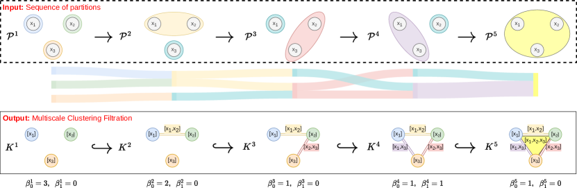
Figure 1: Construction of the MCF. The figure illustrates the construction of the MCF on a set of three points $X=\{x_{1},x_{2},x_{3}\}$ as detailed in Example 4. The top row shows the sequence of partitions partitions $(\mathcal{P}^{t})_{1\leq t\leq 5}$ (and corresponding Sankey diagram) which serves as the input for the MCF and the bottom row shows the filtered simplicial complex $(K^{t})_{1\leq t\leq 5}$. At filtration index $t=4$, the three elements $x_{1}$, $x_{2}$ and $x_{3}$ are in a conflict emerging of three different cluster assignments that produce a non-bounding 1-cycle $[x_{1},x_{2}]+[x_{2},x_{3}]+[x_{3},x_{1}]$ as described in Example 15. The conflict is resolved at index $t=5$ when the 2-simplex $[x_{1},x_{2},x_{3}]$ is added to $K^{5}$.

Remark 5 (Ordering of the sequence of partitions).

Our Example 4 illustrates the key role played by the ordering in the sequence of partitions: swapping partitions $\mathcal{P}^{5}$ and $\mathcal{P}^{1}$ would yield $K^{t}=2^{X}$ for $t\geq 1$ and the filtration cannot incorporate additional information from other partitions. Therefore, MCF is designed to encode sequences of partitions $\theta(t)$ that have an incremental, quasi-hierarchical ordering reflecting a notion of resolution, or coarsening of the partitions across scales. A simple heuristic would be to order the partitions by the number of clusters in decreasing order, i.e., by the dimension of the maximal simplices. This notion reflects the ordering of partitions from fine to coarse obtained in hierarchical and non-hierarchical multiscale clustering algorithms  [79, 65, 80, 85]. Another approach for re-ordering the sequence based on properties of the MCF is presented in Remark 14.

Remark 6.

Example 4 also shows that the MCF is not necessarily 2-determined: although every pair of the set $\{x_{1},x_{2},x_{3}\}$ is a 1-simplex in $K^{4}$, the 2-simplex $[x_{1},x_{2},x_{3}]$ is not included. Hence, the MCF is not a filtered flag complex in general and cannot be constructed as a Vietoris-Rips filtration (Eq. (7)) or clique complex filtration (Eq. (8)), since both are 2-determined.

3.2 Stability of persistence diagrams obtained from the MCF

We are now interested in the persistent homology computed from the MCF $\mathcal{M}$, which can be summarized with the $k$-dimensional persistence diagrams $\operatorname{Dgm}_{k}(\mathcal{M})$ for $0\leq k\leq\dim(K)-1$, where $K=K^{t_{M}}$ as defined in Remark 3. For background on persistent homology see Section 2.2. To prove that the MCF is a well-defined filtration we need to show that its persistence diagram is stable with respect to small perturbations in the sequence of partitions as measured by an adequate metric such as the Wasserstein distance (Eq. (12)).

In order to apply a stability theorem for the Wasserstein distance by [90], we need to find a function $f_{\mathcal{M}}$ that ‘induces’ the filtration $\mathcal{M}=(K^{t})_{t\geq t_{1}}$. We define the function $f_{\mathcal{M}}:K\rightarrow\mathbbm{R}$ for every simplex $\sigma\in K$ as

$$f_{\mathcal{M}}(\sigma)=\min\{t\geq t_{1}\;|\;\exists\;C\in\mathcal{P}^{t}:\;\sigma\subseteq C\},$$ (15)

and it is easy to see that $f_{\mathcal{M}}$ is a filtration function for $\mathcal{M}$, i.e., one recovers the filtration $\mathcal{M}$ from the sublevel sets of $f_{\mathcal{M}}$ by defining

$$K^{t}=f_{\mathcal{M}}^{-1}(-\infty,t).$$ (16)

The filtration function $f_{\mathcal{M}}$ is also simplex-wise monotone, i.e., $f_{\mathcal{M}}(\sigma^{\prime})\leq f_{\mathcal{M}}(\sigma)$ for every $\sigma^{\prime}\subseteq\sigma\in K$ [67].

We can now derive the Wasserstein stability of MCF persistence diagrams.

Proposition 7 (Stability of MCF).

Consider two sequences of partitions with scale functions $\theta:[t_{1},\infty)\rightarrow\Pi_{X}$ and $\tilde{\theta}:[\tilde{t}_{1},\infty)\rightarrow\Pi_{X}$ and corresponding filtrations $\mathcal{M}=(K^{t})_{t\geq t_{1}}$ and $\tilde{\mathcal{M}}=(\tilde{K}^{t})_{t\geq\tilde{t}_{1}}$. If we assume that $K:=\bigcup_{t\geq t_{1}}K^{t}=\bigcup_{t\geq\tilde{t}_{1}}\tilde{K}^{t}$, then, for every $0\leq k\leq\dim(K)-1$,

$$d_{W,q}\left(\operatorname{Dgm}_{k}(\mathcal{M}),\operatorname{Dgm}_{k}(\tilde{\mathcal{M}})\right)^{q}\;\leq\;\sum_{\dim{\sigma}\in\{k,k+1\}}|f_{\mathcal{M}}(\sigma)-f_{\mathcal{\tilde{M}}}(\sigma)|^{q},$$ (17)

where $f_{\mathcal{M}}$ and $f_{\mathcal{\tilde{M}}}$ are the filtration functions of $\mathcal{M}$ and $\mathcal{\tilde{M}}$ respectively and $d_{W,q}$ is the $q$-Wasserstein distance as defined in Eq. (12).

Proof.

The condition $K:=\bigcup_{t\geq t_{1}}K^{t}=\bigcup_{t\geq\tilde{t}_{1}}\tilde{K}^{t}$ guarantees that the two simplex-wise monotone filtration functions $f_{\mathcal{M}}$ and $f_{\mathcal{\tilde{M}}}$ are defined on the same domain $K$ and the proposition then follows directly from the stability theorem for the Wasserstein distance from [90, Theorem 4.8]. ∎

Remark 8.

We can apply the stability result to arbitrary pairs of sequences of partitions defined on the same set of points $X$ by adding the trivial partition $\mathcal{P}=\{X\}$ with a single cluster to the tails of both sequences, i.e. by defining $\theta(t)=\tilde{\theta}(t)=\{X\}$ for $t\gg 1$.

The stability result shows us that we can use the MCF persistence diagrams for the characterisation of multiscale clustering structures. Rather than only comparing pairs of partitions, the MCF allows for the comparison of two whole sequences of partitions using the $q$-Wasserstein distance of their MCF persistence diagrams. Our result is similar to Carlsson and Mémoli’s stability theorem for hierarchical clustering methods [59], which is based on the Gramov-Hausdorff distance between the ultrametric spaces corresponding to two different hierarchical sequences of partitions, but MCF also extends to non-hierarchical sequences of partitions. We will study the stability for the hierarchical case in more detail in Section 5.2.

3.3 Zero-dimensional persistent homology of MCF as a measure of hierarchy

We can now derive theoretical results for the persistent homology of the MCF and start with the zero-dimensional persistent homology. As all vertices in the MCF are born at the same filtration index $t_{1}$, we focus here on the zero-dimensional homology groups $H_{0}^{t}$ of $K^{t}$, $t\geq t_{1}$, directly. First, we provide a definition for the level of hierarchy in a sequence of partitions. We refer to Section 2.1 for background and notation on partitions.

Definition 9 (Non-fractured).

We say that the partition $\mathcal{P}^{t}$ is non-fractured if for all $t_{1}\leq s\leq t$ the partitions $\mathcal{P}^{s}$ are refinements of $\mathcal{P}^{t}$, i.e. $\mathcal{P}^{s}\leq\mathcal{P}^{t}$. We call $\mathcal{P}^{t}$ fractured if this property is not fulfilled.

The partition $\mathcal{P}^{t_{1}}$ is always non-fractured by construction. Note that a sequence of partitions is hierarchical if and only if its partitions $\mathcal{P}^{t}$ are non-fractured for all $t\in\mathbbm{R}$. It turns out that we can quantify the level of hierarchy in the sequence of partitions by comparing the 0-dimensional Betti number $\beta_{0}^{t}$ of the simplicial complex $K^{t}$ with the number of clusters $\#\mathcal{P}^{t}$ at scale $t$.

Proposition 10.

For each $t\geq t_{1}$, the 0-dimensioal Betti number $\beta_{0}^{t}$ fulfills the following properties:

1. $\beta_{0}^{t}\leq\min_{s\leq t}\#\mathcal{P}^{s}$

2. $\beta_{0}^{t}=\#\mathcal{P}^{t}$ if and only if $\mathcal{P}^{t}$ is non-fractured

Proof.

i) The 0-th Betti number $\beta^{t}_{0}$ equals the number of connected components in the simplicial complex $K^{t}$. The complex $K^{t}$ contains the clusters of partitions $\mathcal{P}^{s}$, for $s\leq t$, as solid simplices and the number of these clusters is given by $\#\mathcal{P}^{s}$. This means that $K^{t}$ has at most $\min_{s\leq t}\#\mathcal{P}^{s}$ connected components, i.e. $\beta^{t}_{0}\leq\min_{s\leq t}\#\mathcal{P}^{s}$. ii) “$\Longleftarrow$” Assume first that the partition $\mathcal{P}^{t}$ is non-fractured. This means that the clusters of $\mathcal{P}^{s}$ are nested within the clusters of $\mathcal{P}^{t}$ for all $s\leq t$ and so the maximally disjoint simplices of $K^{t}$ are given by the solid simplices corresponding to the clusters of $\mathcal{P}^{t}$, implying $\beta^{t}_{0}=\#\mathcal{P}^{t}$. “$\Longrightarrow$” Finally consider the case $\beta^{t}_{0}=\#\mathcal{P}^{t}$. Assume that $\mathcal{P}^{t}$ is fractured, i.e. there exist $s<t$ and $x,y\in X$ such that $x\sim_{\mathcal{P}^{s}}y$ but $x\not\sim_{\mathcal{P}^{t}}y$. Then the points $x,y\in X$ are path-connected in $K^{s}$ and because $K^{s}\subseteq K^{t}$, they are also path-connected in $K^{t}$. This implies that the simplices corresponding to the clusters of $x$ and $y$ are in the same connected component. Hence, the number of clusters at $t$ is larger than the number of connected components, i.e. $\beta^{t}_{0}<\#\mathcal{P}^{t}$. This is in contradiction to $\beta^{t}_{0}=\#\mathcal{P}^{t}$ and so $\mathcal{P}^{t}$ must be non-fractured. ∎

The number of clusters $\#\mathcal{P}^{t}$ is thus an upper bound for the Betti number $\beta_{0}^{t}$ and this motivates the following definition.

Definition 11 (Persistent hierarchy).

For $t\geq t_{1}$, the persistent hierarchy is defined as

$$0\leq h(t):=\frac{\beta_{0}^{t}}{\#\mathcal{P}^{t}}\leq 1.$$ (18)

The persistent hierarchy $h(t)$ is a piecewise-constant left-continuous function that measures the degree to which the clusters in partitions up to scale $t$ are nested within the clusters of partition $\mathcal{P}^{t}$ and high values of $h(t)$ indicate a high level of hierarchy in the sequence of partitions. Note that $h(t_{1})=1$ by construction and that always $1/N\leq h(t)$ for all $t\geq t_{1}$. We can use the persistent hierarchy to formulate a necessary and sufficient condition for the hierarchy of a sequence of partitions.

Corollary 12.

$h(t)\equiv 1$ if and only if the sequence of partitions $(\mathcal{P}^{t})_{t\geq t_{1}}$ is strictly hierarchical.

Proof.

“$\Longrightarrow$” For $t\geq t_{1}$, $h(t)=1$ implies that $\mathcal{P}^{t}$ is non-fractured by Proposition 10 ii). Hence, the clusters of partition $\mathcal{P}^{s}$ are nested within the clusters of partition $\mathcal{P}^{t}$ for all $t_{1}\leq s\leq t$ and this means that the sequence of partitions $(\mathcal{P}^{t})_{t\geq t_{1}}$ is strictly hierarchical. “$\Longleftarrow$” A strictly hierarchical sequence implies that $\mathcal{P}^{t}$ is non-fractured for all $t\geq t_{1}$ and hence $h(t)\equiv 1$ by Proposition 10 ii). ∎

We also define the average persistent hierarchy $\bar{h}$ given by

$$\bar{h}:=\frac{1}{t_{M}-t_{1}}\int_{t_{1}}^{t_{M}}h(t)\;dt=\frac{1}{t_{M}-t_{1}}\sum_{m=1}^{M-1}h(t_{m})(t_{m+1}-t_{m}),$$ (19)

to obtain a single measure of hierarchy that takes into account the whole sequence of partitions. While a strictly hierarchical sequence leads to $\bar{h}=1$, our running example shows that a quasi-hierarchical sequence of partitions will still observe high values of $\bar{h}$.

Example 13 (Running example).

Let $(K^{t})_{1\leq t\leq 5}$ be the MCF defined in Example 4. Then the persistent hierarchy is given by $h(1)=h(2)=1$, $h(3)=h(4)=0.5$ and $h(5)=1$. Note that the drop in persistent hierarchy at $t=3$ indicates a violation of hierarchy induced by a conflict between cluster assignments. Yet the high average persistent hierarchy $\bar{h}=0.75$ indicates the presence of quasi-hierarchy in the sequence. As discussed in Remark 5, the ordering of the sequence is crucial and swapping the partitions $\mathcal{P}^{5}$ and $\mathcal{P}^{1}$ would lead to a reduced average persistent hierarchy $\bar{h}=0.58$.

Remark 14.

If the critical values $t_{1}<t_{2}<...<t_{M}$ of $\theta(t)$ are given by integers $1<2<...<M$, one can use the persistent hierarchy to determine a maximally hierarchical ordering of the sequence of partitions. A permutation $\pi$ of $\{1,2,...,M\}$ such that the average persistent hierarchy $\bar{h}$ obtained from the MCF of the sequence $\mathcal{P}^{\pi(1)},\mathcal{P}^{\pi(2)},...,\mathcal{P}^{\pi(M)}$ is maximal leads to such a maximally hierarchical ordering.

3.4 Higher-dimensional persistent homology of MCF as a measure of conflict

For simplicity, we assume in this section that persistent homology is computed over the two-element field $\mathbbm{Z}_{2}$. We will argue that the higher-dimensional persistent homology tracks the emergence and resolution of cluster assignment conflicts across the sequence of partitions. Our running example serves as an illustration.

Example 15 (Running example).

In the setup of Example 4, the three elements $x_{1}$, $x_{2}$ and $x_{3}$ are in a pairwise conflict at $t=4$ because each pair of elements has been assigned to a common cluster but all three elements have never been assigned to the same cluster in partitions up to index $t=4$. This means that the simplicial complex $K^{4}$ contains the 1-simplices $[x_{1},x_{2}]$, $[x_{2},x_{3}]$ and $[x_{3},x_{1}]$ but is missing the 2-simplex $[x_{1},x_{2},x_{3}]$. Hence, the 1-chain $[x_{1},x_{2}]+[x_{2},x_{3}]+[x_{3},x_{1}]$ is a non-bounding 1-cycle that corresponds to the generator of the 1-dimensional homology group $H^{4}_{1}=\mathbbm{Z}$. From Figure 1 we observe that the emergence of the conflict coincides with a crossing in the Sankey diagram. Note that the conflict is resolved at index $t=5$ because the three elements $x_{1}$, $x_{2}$ and $x_{3}$ are assigned to the same cluster in partition $\mathcal{P}^{5}$ and so the simplex $[x_{1},x_{2},x_{3}]$ is finally added to the complex such that there are no more non-bounding 1-cycles and $H^{5}_{1}=0$.

The example motivates a reinterpretation of the cycle-, boundary- and homology groups in terms of cluster assignment conflicts.

Remark 16.

For $t\geq t_{1}$ and dimension $1\leq k\leq\dim(K)-1$ we interpret the elements of the cycle group $Z_{k}^{t}$ as potential conflicts and the elements of the boundary group $B_{k}^{t}$ as resolved conflicts. We then interpret the classes of the persistent homology group $H^{t,p}_{k}$ (Eq. (9)), $p\geq 0$, as equivalence classes of true conflicts that have not been resolved until filtration index $t+p$, and the birth and death times of true conflicts correspond to the times of emergence and resolution of the conflict. Moreover, the total number of unresolved true conflicts at index $t$ is given by the Betti number $\beta_{k}^{t}$.

It is intuitively clear that conflicts only emerge in non-hierarchical sequences of partitions, which is the statement of the next proposition.

Proposition 17.

If the sequence of partitions $(\mathcal{P}^{t})_{t\geq t_{1}}$ is strictly hierarchical, then $H^{t,p}_{k}=0$ for all $1\leq k\leq\dim(K)-1$, $t\geq t_{1}$ and $p\geq 0$.

Proof.

Let $z\in Z^{t}_{k}$ for some $t\geq t_{1}$ and $1\leq k\leq\dim(K)-1$ and let $m\leq M$ be the largest $m$ such that $t_{m}\leq t$, i.e. $K^{t}=K^{t_{m}}$. Then there exist $k$-simplices $\sigma_{1},...,\sigma_{n}\in K^{t}$, $n\in\mathbbm{N}$, such that $z=\sigma_{1}+...+\sigma_{n}$. In particular, for all $i=1,...,n$ exist $m(i)\leq m$ such that for all $x,y\in\sigma_{i}$ we have $x\sim_{t_{m(i)}}y$. As the sequence of partitions is hierarchical, $x\sim_{{t_{m(i)}}}y$ for some $x,y\in X$ implies that $x\sim_{{t_{m}}}y$ and so for all $x,y\in\bigcup_{i=1}^{n}\sigma_{i}$ we have $x\sim_{t_{m}}y$. This means that $\bigcup_{i=1}^{n}\sigma_{i}\in K^{t}$ and so there exists a $c\in C^{t}_{k+1}$ such that $\partial_{k+1}c=z$. Hence, $Z^{t}_{k}\subseteq B^{t}_{k}$ which proves $H^{t,p}_{k}=0$ for all $p\geq 0$. ∎

In non-hierarchical sequences of partitions, we can thus analyse the birth and death times of higher-dimensional homology classes to trace the emergence and resolution of cluster assignment conflicts across scales. Recall that the number of $k$-dimensional homology classes with birth time $s$ and death time $t\geq s$ is given by $\mu_{k}^{s,t}$, the multiplicity of point $(s,t)$ in the $k$-dimensional persistence diagram $\operatorname{Dgm}_{k}(\mathcal{M})$ (see Eq. (10)). Using these multiplicities allows us to quantify how many conflicts are created or resolved at a certain scale and following Remark 3, it is sufficient to only consider the critical values $t_{1}<t_{2}<...<t_{M}$ of the scale function $\theta(t)$ as those scales where the homology changes.

Definition 18.

A partition $\mathcal{P}^{t_{m}}$ is conflict-creating if the number of independent $k$-dimensional classes that are born at filtration index $t_{m}$ is larger than 0, i.e.,

$$b_{k}(t_{m}):=\sum_{l=m+1}^{M}\mu_{k}^{t_{m},t_{l}}+\mu_{k}^{t_{m},\infty}>0.$$ (20)

Similarly, a partition $\mathcal{P}^{t_{m}}$ is conflict-resolving if the number of independent $k$-dimensional classes that die at filtration index $t_{m}$ is larger than 0, i.e.,

$$d_{k}(m):=\sum_{l=1}^{m-1}\mu_{k}^{t_{l},t_{m}}>0.$$ (21)

Of course, a partition can be both conflict-creating and conflict-resolving and so a good partition is a partition that resolves many conflicts and creates few new conflicts.

Definition 19 (Persistent conflict).

The persistent conflict for dimension $1\leq k\leq\dim(K)-1$ at level $t_{m}$, $m\leq M$, is defined as

$$c_{k}(t_{m}):=b_{k}(t_{m})-d_{k}(t_{m}),$$ (22)

and the total persistent conflict is the sum

$$c(t_{m}):=\sum_{k=1}^{\dim(K)-1}c_{k}(t_{m}).$$ (23)

We now show that the persistent conflict $c_{k}(t_{m})$, $m\leq M$, can be interpreted as the discrete derivative of the Betti number $\beta_{k}^{t_{m}}$.

Proposition 20.

For all $1\leq k\leq\dim(K)-1$ we have:

1. $c_{k}(t_{1})=b_{k}(t_{1})$ and $c_{k}(t_{m})=\Delta\beta^{t_{m-1}}_{k}:=\beta^{t_{m}}_{k}-\beta^{t_{m-1}}_{k}$ for $2\leq m\leq M$, where $\Delta$ denotes the forward difference operator,

2. $\beta_{k}^{t_{m}}=\sum_{l=1}^{m}c_{k}(t_{l})$ for all $m\leq M$.

Proof.

Statement ii) is a simple consequence of the Fundamental Lemma of Persistent Homology (Eq. (11)). To prove i), notice that always $d_{k}(1)=0$ and so $c_{k}(1)=b_{k}(1)$. Then the rest follows directly from ii). ∎

We can extend the (total) persistent conflict to a piecewise-constant left-continuous function $c(t)$ on $t\geq t_{1}$ by interpolation between the critical values $t_{1}<t_{2}<...<t_{M}$.

Remark 21.

Following our heuristics, good conflict-resolving partitions are then located at plateaus after dips of the $c(t)$, which also correspond to gaps in the death-dimension of the persistence diagram. Additionally, the total number of unresolved conflicts at scale $t$ given by the Betti number $\beta_{k}^{t}$ should be low for all dimensions $1\leq k\leq\dim(K)-1$.

We finally show that the dimension $1\leq k\leq\dim(K)-1$ can give us insights into the kind of “conflict parties” involved in a cluster assignment conflict.

Remark 22.

The dimension of the conflict in our running example is $k=1$ because it emerges as a conflict of pairwise cluster assignment conflicts, where the “conflict parties” are pairs of elements of $X$ that were clustered together such that overlap exists across scales and a cycle emerges in the MCF, see Example 15. Note that a one-dimensional conflict can be formed by many of such “conflict parties” (because cycles can have a large diameter in homology) but the parties themselves always consist of two elements. In contrast, higher dimensional conflicts for $k>1$ involve “conflict parties” of larger size $k+1$. One could thus argue that conflicts get more severe with larger dimensions. However, we can only observe these higher-dimensional conflicts when the clusters in the sequence of partitions become large enough and so one should compare the dimension of the conflict also with the size of the clusters.

4 Numerical experiments

In this section, we present numerical experiments where the MCF framework is applied to synthetic data sampled from four stochastic block models with different intrinsic structure: (i) an Erdös-Renyi (ER) model (no intrinsic scale) [70, 53]; (ii) a single-scale Stochastic Block Model (SBM) (one scale) [72, 77]; (iii) a multiscale SBM (multiple scales, hierarchical) [84, 50, 87]; and (iv) a non-hierarchical multiscale SBM (multiple scales, non-hierarchical). Each of the four models can also be thought of as an unweighted and undirected random graph $G_{i}=(V,E_{i})$, $i=1,2,3,4$, defined over the same vertex set $V=\{1,2,...,270\}$ and with a similar number of edges of about $3,500$. To generate the multiscale clusterings, we use the Markov Stability (MS) algorithm for multiscale community detection [79, 65, 80, 85, 50]. MS produces a non-hierarchical multiscale sequence of partitions $\theta_{i}:[t_{1},t_{200}]\rightarrow\Pi_{V}$ such that $t\mapsto\mathcal{P}_{i}^{t}$, where $\mathcal{P}_{i}^{t}$ is a partition of $V$ for each graph $G_{i}$, $i=1,2,3,4$, indexed over the continuous Markov time $t$, which is evaluated at 200 scales equidistantly ranging from $t_{1}=-1.5$ to $t_{200}=0.5$. The finest partition $\mathcal{P}_{i}^{t_{1}}$ is always the partition of singletons and the partitions get coarser as $t$ increases. In Appendix B, we give more details about the stochastic block models and Figure 7 visualises the adjacency matrix of the associated random graphs and the Sankey diagram for each sequence of partitions.

It is important to remark that, in contrast to hierarchical clustering, MS does not impose a hierarchical assumption on the sequence of partitions. As a consequence, the MS multiscale clusterings of a stochastic hierarchical model (like the multiscale SBM) will not be strictly hierarchical due to stochastic variability in the sampling. However, the planted hierarchical structure will emerge as robust partitions through our MCF analysis.

From each sequence $\theta_{i}:[t_{1},t_{200}]\rightarrow\Pi_{V}$, $i=1,2,3,4$, we obtain the MCF $\mathcal{M}_{i}=(K_{i}^{t})_{t\geq t_{1}}$ defined on the same set of vertices $V$ and with continuous filtration index $t\geq t_{1}$ interpolating between the Markov times in $T$. We use the GUDHI software [51] for the computation of persistent homology of the MCF, where we restrict ourselves to dimensions $k\leq 2$, and compute our measure of persistent hierarchy (Eq.(18)) and total persistent conflict (Eq. (23)). We also compare the sequence of partitions with the ground truth a posteriori (shaded in pink in the figures).

ER model

The persistence diagram of the ER model [70, 53] in Figure 2A shows no distinctive gaps in the death times confirming the absence of any scales or blocks in the data (Remark 21). Further, the low values of the persistent hierarchy $h(t)$ (Figure 2B) for an average persistent hierarchy $\bar{h}=0.30$ indicates a lack of hierarchy in the sequence of partitions obtained with MS. This is expected given the fact that there are no robust partitions at any scale in the ER model, hence the sequence of partitions extracted by MS has no natural quasi-hierarchical ordering. Following the heuristics in Section 3.4, the sequence contains no good conflict-resolving partition because the plateaus after dips in the total persistent conflict $c(t)$ are located at scales where still a large number of conflicts are unresolved. This is indicated by the large one-dimensional Betti number $\beta_{1}^{t}$ for $t>0$ and the many one-dimensional points at infinity in the persistence diagram, respectively. We also observe two-dimensional conflicts, i.e. “conflicts involving larger parties”, emerging at larger scales $t>0$ of which most remain unresolved in the absence of a good conflict-resolving partition. These findings reinforce the lack of robust partitions in the ER model.

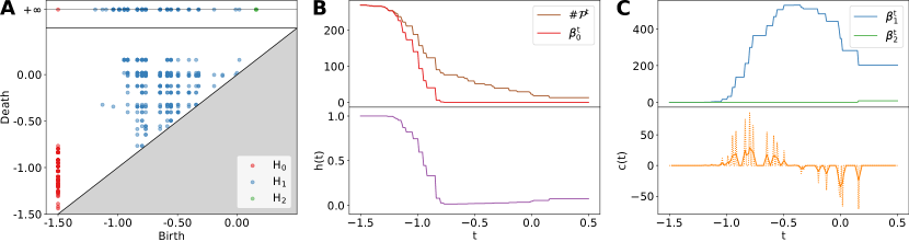
Figure 2: MCF applied to multiscale clustering of ER. A We compute the persistence diagram of the MCF constructed from the sequence of partitions $\theta_{1}$ obtained from the ER graph. B The persistent hierarchy $h(m)$ (18) drops quickly without recovery indicating that the sequence is strongly non-hierarchical. C The total persistent conflict $c(m)$ (23) has no distinct plateaus after dips that correspond to low values of the Betti numbers $\beta_{1}^{t}$ and $\beta_{2}^{t}$ indicating the absence of a good conflict resolving partition.

Single-scale SBM

The single-scale SBM has a planted partition into three equal-sized clusters (also called blocks) [72, 77]. The persistence diagram of the SBM in Figure 3A shows a distinct gap after $t=-0.15$ which is shown a posteriori to correspond to the ground truth partition. After an initial decrease, the persistent hierarchy $h(t)$ recovers (Figure 3B), indicating the presence of some quasi-hierarchy at the large scale in the sequence of partitions (average persistent hierarchy of $\bar{h}=0.41$). Note, however, that $h(t)$ does not approach 1 due to the randomness of the SBM model with non-zero cross-block probability. The total persistent conflict in Figure 3C reveals a good conflict-resolving partition, located both at a distinct plateau after dips in the total persistent conflict $c(t)$ and at low Betti numbers $\beta_{1}^{t}$ and $\beta_{2}^{t}$. We identify this scale a posteriori as recovering the ground truth partition. Note, that this robust partition resolves the two-dimensional conflicts (in contrast to the ER where they remained unresolved).

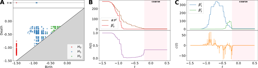
Figure 3: MCF applied to multiscale clustering of single-scale SBM. A We compute the persistence diagram of the MCF constructed from the sequence of partitions $\theta_{2}$ obtained from the SBM. B The persistent hierarchy $h(t)$ (18) recovers after an initial decrease indicating the presence of quasi-hierarchy in the sequence. C The total persistent conflict $c(t)$ (23) has a distinct plateau from about $t=0$ following dips in $c(t)$ located at low values of the Betti numbers $\beta_{1}^{t}$ and $\beta_{2}^{t}$.

Multiscale SBM

The multiscale SBM [84, 50, 87] has ground truth partitions planted at three different scales with 27, 9, and 3 equal-sized blocks, respectively, with blocks of the fine scale nested within blocks of the medium scale, in turn nested in blocks of the coarse scale. The MCF in this case exhibits a distinct clustering of birth-death tuples in the persistence diagram, and we find a posteriori that the gaps in the death time correspond to the three intrinsic scales in the model (Figure 4A). This effect is also reflected in the total persistent conflict $c(t)$ in Figure 4C, whose three distinct plateaus correspond to the three planted partitions at different scales. The high values of the persistent hierarchy $h(t)$ close to 1 indicate a strong degree of quasi-hierarchy in the sequence of partitions (Figure 4B) with a high average persistent hierarchy $\bar{h}=0.73$. Again, although the multiscale SBM is statistically hierarchical, the sequence of partitions obtained by MS is not strictly hierarchical due to random variability in the sample, hence $\bar{h}\neq 1$.

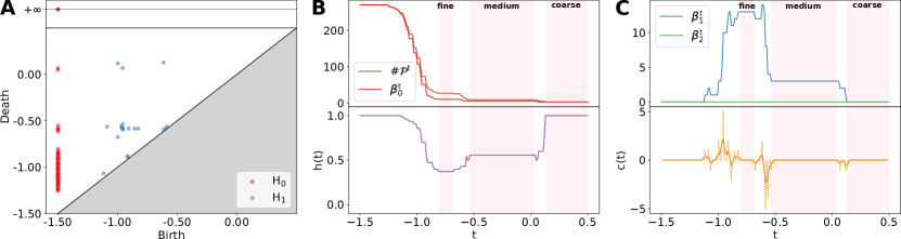
Figure 4: MCF applied to multiscale clustering of multiscale SBM. A The persistence diagram of the MCF constructed from the sequence of partitions $\theta_{3}$ obtained from the multiscale SBM shows three distinct gaps corresponding to the ground truth partitions. B The persistent hierarchy $h(t)$ (18) remains relatively high throughout the sequence of partitions indicating a strong degree of quasi-hierarchy. C The total persistent conflict $c(t)$ (23) has three distinct plateaus following dips located at low values of the Betti number $\beta_{1}^{t}$ showing that the ground truth partitions are good conflict-resolving partitions.

Non-hierarchical multiscale SBM

Finally, the non-hierarchical multiscale SBM has a ground truth structure at 3 planted scales with 27, 5, and 3 equal-sized blocks, respectively, yet the blocks of the fine scale are not nested into the blocks of the medium scale, which are again not nested into the blocks of the coarse scale. The analysis of the MCF shows reduced values of the persistent hierarchy $h(t)$ (Figure 5B) indicating a lower degree of quasi-hierarchy in the sequence of partitions (average persistent hierarchy $\bar{h}=0.45$) due to the data being sampled from a non-hierarchical model. However, we still observe a distinct clustering of birth-death tuples in the persistence diagram with gaps in the death time corresponding to the three intrinsic scales of the graph (Figure 5A). The total persistent conflict $c(t)$ in Figure 5C shows three distinct plateaus corresponding to these three planted partitions at different scales.

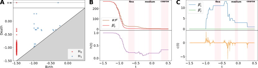
Figure 5: MCF applied to multiscale clustering of non-hierarchical multiscale SBM. A The persistence diagram of the MCF constructed from the sequence of partitions $\theta_{4}$ obtained from the non-hierarchical multiscale SBM shows three distinct gaps corresponding to the ground truth partitions. B The persistent hierarchy $h(t)$ (18) is reduced throughout the sequence of partitions indicating a lower degree of quasi-hierarchy. C The total persistent conflict $c(t)$ (23) has three distinct plateaus following dips located at low values of the Betti number $\beta_{1}^{t}$ showing that the ground truth partitions are good conflict-resolving partitions.

In summary, our numerical experiments show that the MCF persistence diagram provides a rich summary for different sequences of partitions. The derived measure of persistent hierarchy quantifies the level of hierarchy present in the sequence of partitions, reflecting the planted hierarchical structure. Furthermore, the total persistent conflict identifies the ground truth scales (present in the different versions of SBMs) as resolving many conflicts.

5 Mathematical links of MCF to other filtrations

In this section, we explore the connection of MCF to alternative constructions of filtered abstract simplicial complexes from a sequence of partitions $\theta:[t_{1},\infty)\rightarrow\Pi_{X}$ of a set $X$.

5.1 Equivalent construction of the MCF based on nerve complexes

We first construct a novel filtration from a sequence of partitions based on nerve complexes, inspired by the MAPPER construction [89]. For notational convenience, we assume in this section that the sequence of partitions is indexed by a simple enumeration, i.e. $(\mathcal{P}^{m})_{1\leq m\leq M}$, but all results also extend to the case of a continuous scale function $\theta(t)$ as defined in Eq. (1).

Definition 23.

Let $\mathcal{C}(m)=(C_{\alpha})_{\alpha\in A(m)}$ for $1\leq m\leq M$ be the family of clusters indexed over the multi-index set $A(m)=\{(m^{\prime},i)\;|\;1\leq m^{\prime}\leq m,\;i\leq\#\mathcal{P}^{m^{\prime}}\}$ such that $C_{(m,i)}$ is the $i$-th cluster in partition $\mathcal{P}^{m}$. Then we define the Multiscale Clustering Nerve (MCN) $N^{m}$ as the nerve complex of $\mathcal{C}(m)$, i.e. $N^{m}=\left\{S\subseteq A(m):\bigcap_{\alpha\in S}C_{\alpha}\neq\emptyset\right\}$ [82].

The abstract simplicial complex $N^{m}$ records the intersection patterns of all clusters up to partition index $m$ and using these nested complexes we can obtain the Multiscale Clustering Nerve Filtration (MCNF) $\mathcal{N}=(N^{m})_{1\leq m\leq M}$, which provides a complementary perspective to the MCF. While the vertices of $\mathcal{M}$ correspond to points in $X$ and the generators of conflicts inform us about which points are at the boundaries of clusters, the vertices of $\mathcal{N}$ correspond to clusters in the sequence of partitions $(\mathcal{P}^{m})_{1\leq m\leq M}$ and the generators of conflicts inform us about which clusters lead to a conflict. We illustrate the construction of the MCNF with our running example in Figure 6.

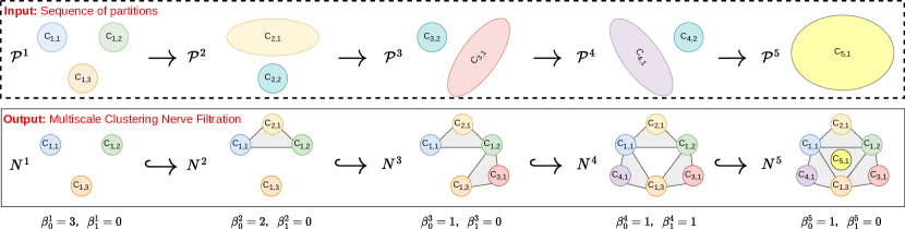
Figure 6: Construction of the MCNF. The figure illustrates the construction of the MCNF on our running Example 4 and the top row shows the sequence of partitions $(\mathcal{P}^{t})_{1\leq t\leq 5}$, where we indexed the clusters as described above. The bottom row shows the MCNF $(N^{t})_{1\leq t\leq 5}$, where we only labeled the 0-simplices and for $N^{5}$ we simplify the visualisation. Note that the Betti numbers match with those of the MCF construction, see Figure 1, but the MCNF leads to a filtration with a larger number of simplices.

It is no coincidence that the MCNF construction leads to the same Betti numbers in our running example as obtained with the MCF. In fact, it turns out that both filtrations actually lead to the same persistent homology and to prove this we first adapt the Persistent Nerve Lemma by [64] to abstract simplicial complexes.

Lemma 24.

Let $K\subseteq K^{\prime}$ be two finite abstract simplicial complexes, and $\{K_{\alpha}\}_{\alpha\in A}$ and $\{K^{\prime}_{\alpha}\}_{\alpha\in A}$ be subcomplexes that cover $K$ and $K^{\prime}$ respectively, based on the same finite parameter set such that $K_{\alpha}\subseteq K^{\prime}_{\alpha}$ for all $\alpha\in A$. Let further $N$ denote the nerve $\mathcal{N}\left(\{|K_{\alpha}|\}_{\alpha\in A}\right)$ and $N^{\prime}$ the nerve $\mathcal{N}\left(\{|K^{\prime}_{\alpha}|\}_{\alpha\in A}\right)$. If for all $k\in\mathbbm{N}$ and for all $\alpha_{0},...,\alpha_{k}\in A$ the intersections $\bigcap_{i=0}^{k}|K_{\alpha_{i}}|$ and $\bigcap_{i=0}^{k}|K^{\prime}_{\alpha_{i}}|$ are either empty or contractible, then there exist homotopy equivalences $N\rightarrow|K|$ and $N^{\prime}\rightarrow|K^{\prime}|$ that commute with the canonical inclusions $|K|\hookrightarrow|K^{\prime}|$ and $N\hookrightarrow N^{\prime}$.

A proof of Lemma 24 can be found in Appendix A. We are now ready to prove the equivalence of the persistent homology of the MCF and the MCNF.

Proposition 25.

For $k\geq 0$, $1\leq m\leq M$ and $p\geq 0$ such that $m+p\leq M$ we have $H_{k}^{p}(N^{m})\cong H_{k}^{p}(K^{m})$.

Proof.

Using Lemma 24, we show that there exist homotopy equivalences $N^{m}\rightarrow|K^{m}|$ and $N^{m+p}\rightarrow|K^{m+p}|$ that commute with the canonical inclusions $|K^{m}|\hookrightarrow|K^{m+p}|$ and $N^{m}\hookrightarrow N^{m+p}$. This leads to the following commutative diagram on the level of homology groups:

where the vertical arrows are group isomorphisms and the horizontal arrows $f_{N}$ and $f_{K}$ are the homomorphisms induced by the canonical inclusions. The proposition then follows with the observation that

$$H_{k}^{p}(N^{m})=\operatorname{im}{f^{m,m+p}_{N}}\cong\operatorname{im}{f^{m,m+p}_{K}}=H_{k}^{p}(K^{m}).$$ (24)

To show that the requirements for Lemma 24 are satisfied, let us first denote $K:=K^{m}$, $K^{\prime}:=K^{m+p}$, $N:=N^{m}$ and $N^{\prime}=N^{m+p}$. For the index set $A=A(m^{\prime})$, define the covers $\{K_{\alpha}\}_{\alpha\in A}$ and $\{K^{\prime}_{\alpha}\}_{\alpha\in A}$ by $K_{\alpha}=\Delta C_{\alpha}$ if $\alpha\in A(m)\subseteq A$ and $K_{\alpha}=\emptyset$ otherwise and $K^{\prime}_{\alpha}=\Delta C_{\alpha}$ for all $\alpha\in A$. Then we have $K_{\alpha}\subseteq K^{\prime}_{\alpha}$ for all $\alpha\in A$ and we recover the MCF $K=\bigcup_{\alpha\in A}K_{\alpha}$ and the MCNF $N=\mathcal{N}\left(\{K^{\prime}_{\alpha}\}_{\alpha\in A}\right)$ and similarly we recover $K^{\prime}$ and $N^{\prime}$. It remains to show that for any $k\in\mathbbm{N}$ and $\alpha_{0},...,\alpha_{k}\in A$ the intersections $\bigcap_{i=0}^{k}|K^{\prime}_{\alpha_{i}}|$ are either empty or contractible. This is true because if $D=\bigcap_{i=0}^{k}|K^{\prime}_{\alpha_{i}}|\neq\emptyset$, then $D$ is the intersection of solid simplices and thus a solid simplex itself. ∎

The proposition shows us that the point-centered perspective of the MCF and the cluster-centered perspective of the MCNF are essentially equivalent. The proposition also has computational consequences.

Remark 26.

If the total number of clusters is smaller than the size of $X$, i.e. $\sum_{m=1}^{M}\#\mathcal{P}^{m}<\#X$, then it is computationally beneficial to use the MCNF instead of the MCF. However, we often have the case that $\mathcal{P}^{1}$ is a partition of singletons, i.e. $\#\mathcal{P}^{1}=\#X$, and then MCF should be preferred for computational reasons.

5.2 MCF in the special case of hierarchical clustering

Next, we define an adjacency matrix from the sequence of partitions $\theta:[t_{1},\infty)\rightarrow\Pi_{X},t\mapsto\mathcal{P}^{t}$ whose clique complex filtration is (only) equivalent to the MCF in the hierarchical case.

Definition 27.

The undirected and weighted Cluster Assignment Graph (CAG) $G=(V,E)$ with nodes $V=X$ is defined through its $N\times N$ adjacency matrix $A$ given by:

$$A_{xy}=\min\left\{t\geq t_{1}|\;x\sim_{t}y\right\},$$ (25)

where $A_{xy}$ is the scale of the first partition where data points $x$ and $y$ are part of the same cluster. We define $\min\emptyset=0$ to ensure that nodes $x$ and $y$ are not linked together if they are never part of the same cluster.

The adjacency matrix $A$ is symmetric with diagonal values given by $t_{1}$, and so it fulfils the properties of a dissimilarity measure ($A_{xx}\leq A_{xy}=A_{yx}$ for all $x,y\in X$) [63]. In the case of hierarchical clustering, $A$ also fulfils the strong triangle-inequality ($A_{xz}\leq\max(A_{xy},A_{yz})$ for all $x,y,z\in X$) because it is in fact equivalent to the ultrametric associated to the dendrogram of the sequence of partitions defined by [59]. In the case of a non-hierarchical sequence, however, $A$ does not even fulfil the standard triangle inequality in general.

We can define a simplicial complex $L^{t}$, $t\geq t_{1}$, given by the clique complex of the thresholded CAG $G_{t}=(V,E_{t})$, which only contains edges $\{x,y\}\in E_{t}\subseteq E$ with $A_{xy}\leq t$, see Section 2.2. The clique complex filtration $\mathcal{L}=(L^{t})_{t\geq t_{1}}$ guarantees the stability of persistence diagrams because $A$ is a dissimilarity measure [63]. However, $\mathcal{L}$ is not equivalent to the MCF $\mathcal{M}$ and leads to a different persistent homology as one can see from our running example.

Example 28 (Running example).

While $K^{t}=L^{t}$ for $t\leq 3$ we have $K^{4}\neq L^{4}=2^{X}$ because $L^{4}$ is the clique complex corresponding to the undirected graph $G_{4}$ with adjacency matrix

$$A=\begin{pmatrix}0&2&0\\ 0&0&3\\ 4&0&0\end{pmatrix},$$ (26)

where $[x_{1},x_{2},x_{3}]$ is already contained as a clique. This means that the one-dimensional homology group $H^{4}(L^{4})$ is trivial and so $\mathcal{L}$ leads to a different persistent homology.

The example shows that the CAG is less sensible to the emergence and resolution of conflicts and also reflects the observation from Section 3.1 that the MCF is not 2-determined and thus cannot be constructed as a clique complex filtration. We can still show that $\mathcal{L}$ has the same zero-dimensional persistent homology as $\mathcal{M}$, implying that we can at least compute the persistent hierarchy $h(t)$ (Eq. (18)) from $\mathcal{L}$.

Proposition 29.

For $t\geq t_{1}$ and $p\geq 0$ we have $H_{0}^{p}(L^{t})=H_{0}^{p}(K^{t})$ but the equality $H_{k}^{p}(L^{t})=H_{k}^{p}(K^{t})$ does not hold for $1\leq k\leq\dim(K)-1$ in general.

Proof.

For each $t\geq t_{1}$, the 1-skeletons of $L^{t}$ and $K^{t}$ are equivalent and so $H_{0}^{p}(L^{t})=H_{0}^{p}(K^{t})$ for all $p\geq 0$. As $L^{t}$ is 2-determined but $K^{t}$ not, the equality $H_{k}^{p}(L^{t})=H_{k}^{p}(K^{t})$ does not hold for $1\leq k\leq\dim(K)-1$ in general. ∎

In the case of a strictly hierarchical sequence of partitions, $\mathcal{L}$ is equivalent to the Vietoris-Rips filtration of the ultrametric space $(X,A)$ and we can show that it leads to the same persistent homology as the MCF.

Corollary 30.

If the sequence of partitions $(\mathcal{P}^{t})_{t\geq t_{1}}$ is strictly hierarchical, then $H_{k}^{p}(L^{t})=H_{k}^{p}(K^{t})$ for all $k\leq\dim(K)-1$, $t\geq t_{1}$ and $p\geq 0$.

Proof.

From the previous proposition we already know that the zero-dimensional persistent homology groups of $\mathcal{L}$ and $\mathcal{M}$ are equivalent. Using Proposition 17, it thus remains to show that $H_{k}^{p}(L^{t})=0$ for all $1\leq k\leq\dim(K)-1$, $t\geq t_{1}$ and $p\geq 0$. As $(\mathcal{P}^{t})_{t\geq t_{1}}$ is strictly hierarchical, the adjacency matrix $A$ of the CAG (Eq. (25)) corresponds to an ultrametric. We complete the proof by recalling that the higher-dimensional homology groups of a Vietoris-Rips filtration constructed from an ultrametric space are zero, see [92]. ∎

Analysing hierarchical clustering with the MCF $\mathcal{M}$ is thus equivalent to analysing the ultrametric space $(X,A)$ associated with the dendrogram with a Vietoris-Rips filtration. If we assume that the hierarchical sequence of partitions was obtained from a finite metric space $(X,d)$ using single linkage hierarchical clustering, we can use the stability theorem by [59] to relate the (only non-trivial) zero-dimensional persistence diagram of the MCF directly to the underlying space.

Corollary 31 (MCF stability for single linkage hierarchical clustering).

Let $\theta:[0,\infty)\rightarrow\Pi_{X}$ and $\tilde{\theta}:[0,\infty)\rightarrow\Pi_{Y}$ be two sequences of partitions obtained from the finite metric spaces $(X,d_{X})$ and $(Y,d_{Y})$ respectively using single linkage hierarchical clustering. Then we obtain the following inequalities for the corresponding MCFs $\mathcal{M}$ and $\tilde{\mathcal{M}}$ and ultrametrics $A$ and $\tilde{A}$:

(27)

where $d_{W,\infty}$ (Eq. (13)) refers to the bottleneck distance and $d_{\text{GH}}$ to the Gromov-Hausdorff distance.

Proof.

Single linkage hierarchical clustering produces strictly hierarchical sequences of partitions and so $A$ and $\tilde{A}$, the adjacency matrices of the CAGs associated to the MCFs $\mathcal{M}$ and $\tilde{\mathcal{M}}$ as defined in Eq. (25), are ultrametrics. The second inequality thus follows the stability result for single linkage hierarchical clustering by [59, Proposition 26], because $A$ and $\tilde{A}$ are equivalent to the ultrametrics associated to the dendrograms of the sequences of partitions obtained from single linkage hierarchical clustering.

Furthermore, one can interpret the clique complex filtrations $\mathcal{L}$ and $\mathcal{L}^{\prime}$ derived from $A$ and $\tilde{A}$ as Vietoris-Rips filtrations defined on the finite ultrametric spaces $(X,A)$ and $(X,\tilde{A})$, respectively. Following a standard stability result for the Vietoris-Rips filtration [62, Theorem 3.1] we get

$$d_{W,\infty}\left(\operatorname{Dgm}_{0}(\mathcal{L}),\operatorname{Dgm}_{0}(\tilde{\mathcal{L}})\right)\;\leq\;d_{\text{GH}}((X,A),(Y,\tilde{A})).$$

The first inequality then follows because Corollary 30 implies that the persistence diagrams for the MCF and the clique complex filtration of the CAG are the same. ∎

The previous result shows that zero-dimensional persistence diagrams of the MCF can serve as an additional tool for the comparison of dendrograms emerging from (single linkage) hierarchical clustering, which is equivalent to using the Vietoris-Rips filtration on the associated ultrametric spaces.

6 Conclusion

In this article, we develop a TDA-based framework for the analysis and comparison of (non-hierarchical) sequences of partitions that arise in multiscale clustering applications. We define a novel filtration, the Multiscale Clustering Filtration (MCF), which encodes arbitrary patterns of cluster assignments across scales, and we prove that the MCF is a proper filtration of abstract simplicial complexes that produces a stable persistence diagram. We use the zero-dimensional persistent homology of the MCF to define a measure for the hierarchy in the sequence of partitions called persistent hierarchy. We also show that the higher-dimensional persistent homology tracks the emergence and resolution of conflicts between cluster assignments across scales, and we define the measure of persistent conflict to identify partitions that resolve many conflicts. In our numerical experiments, we illustrate how the MCF persistence diagram and our derived measures can characterise multiscale data clusterings and identify ground truth partitions, if existent, as those resolving many conflicts.

While multiscale clusterings have been tackled with TDA-based methods before, these were limited to the hierarchical case. Motivated by Multiscale MAPPER [66], an algorithm that produces a hierarchical sequence of representations at multiple levels of resolution, the notion of ‘Topological Hierarchies’ was developed to study tree structures emerging from hierarchical clustering [54, 55]. Similar objects (e.g., merge trees, branching morphologies or phylogenetic trees) have also been studied with topological tools and their structure can be distinguished using persistent barcodes [75, 76]. In contrast, our setting is closer to the study of phylogenetic networks with horizontal evolution across lineages [61], and the MCF is applicable to both hierarchical and non-hierarchical multiscale clustering. The MCF can thus be interpreted as a tool to study more general Sankey diagrams (rather than only strictly hierarchical dendrograms) that emerge naturally from multiscale data analysis. A related framework for the analysis of dynamic graphs was developed by Kim and Mémoli who define so-called ‘formigrams’ that lead to ‘zigzag’ diagrams of partitions [78], but a detailed comparison lies beyond the scope of this article and deserves further work.

Several additional open research directions deserve further work. One goal is to compute minimal generators of the MCF persistent homology classes to locate not only when but also where conflicts emerge in the dataset. Furthermore, we are currently working on a bootstrapping scheme for MCF inspired by [57] that would enable the application of MCF to larger data sets; yet, while first experimental results are promising, a theoretical underpinning and estimation of error rates still need to be established.

Declarations

Ethical Approval

No ethics approval was required.

Competing interests

The authors declare that they have no competing interests.

Authors’ contributions

DS developed the theoretical analysis, performed the computations in this study, prepared the figures and wrote the main manuscript text. Both authors contributed to the design of the research and the revision of the work and the manuscript.

Funding

DS acknowledges support from the EPSRC (PhD studentship through the Department of Mathematics at Imperial College London). MB acknowledges support from EPSRC grant EP/N014529/1 supporting the EPSRC Centre for Mathematics of Precision Healthcare.

Availability of data and materials

A python implementation of MCF based on the GUDHI software [51] is hosted on GitHub under a GNU General Public License at https://github.com/barahona-research-group/MCF. The repository also contains code to reproduce our numerical experiments. The multiscale clusterings were obtained using Markov Stability using the PyGenStability python package [50] available at https://github.com/barahona-research-group/PyGenStability.

Acknowledgements

We thank Heather Harrington for helpful discussions and for the opportunity to present work in progress at the Oxford Centre for Topological Data Analysis in January 2023. We also thank Iris Yoon and Lewis Marsh for valuable discussions. This work has benefited from the first author’s participation in Dagstuhl Seminar 23192 “Topological Data Analysis and Applications”.

Appendix A: Proof of Persistent Nerve Lemma for abstract simplicial complexes

Proof of Lemma 24.

Let $K^{\prime}$ be an abstract simplicial $p$-complex with $N$ vertices, then we use the canonical geometric realisation in $(\mathbbm{R}^{N},d)$ that maps the $k$-th vertex $v_{k}$ to the $k$-th canonical basis vector $e_{k}$, and where $d$ is the standard Euclidian distance. We can compute a geometric realisation of $K\subseteq K^{\prime}$ with the same map and so the underlying spaces fulfil $|K|\subseteq|K^{\prime}|\subseteq\mathbbm{R}^{N}$. Also observe that for any $\sigma,\tau\in K^{\prime}$ we have

$$|\sigma|\cap|\tau|=\emptyset\iff d(|\sigma|,|\tau|)\geq d_{\min}:=\frac{1}{\sqrt{p+1}},$$ (28)

where $p$ is the maximum dimension of any simplex in $K^{\prime}$. This is true because $|\sigma|\cap|\tau|$ implies that $|\sigma|$ and $|\tau|$ are orthogonal sets in $\mathbbm{R}^{N}$ and so $d(|\sigma|,|\tau|)=\min_{x\in|\sigma|,y\in|\tau|}\sqrt{||x||^{2}+||y||^{2}}\geq\min_{x\in|\sigma|}||x||$ and because every $x\in|\tau|$ is a convex combination of at least $p+1$ basis vectors we have $||x||\geq\frac{1}{\sqrt{p+1}}$.

Let $\mathcal{B}_{r}(\cdot)$ denote the open ball in $|K|\subseteq\mathbbm{R}^{N}$ with radius $r:=\frac{d_{\min}}{3}>0$ centred around a point (or a subset) and for $\alpha\in A$ we define the open ‘inflation’ of $|K_{\alpha}|$ in $|K|$ as

$$U_{\alpha}=\mathcal{B}_{r}(|K_{\alpha}|)=\bigcup_{x\in|K_{\alpha}|}\mathcal{B}_{r}(x).$$

Then $\mathcal{U}=\{U_{\alpha}\}_{\alpha\in A}$ is an open cover for $|K|$ and a similar construction leads to the open cover $\mathcal{U}^{\prime}=\{U^{\prime}_{\alpha}\}_{\alpha\in A}$ for $|K^{\prime}|$ such that $U_{\alpha}\subseteq U^{\prime}_{\alpha}$ for all $\alpha\in A$. Moreover, for all $k\in\mathbbm{N}$ and $\alpha_{0},...,\alpha_{k}\in A$ it holds that

$$\bigcap_{i=0}^{k}U_{\alpha_{i}}=\mathcal{B}_{r}\left(\bigcap_{i=0}^{k}|K_{\alpha_{i}}|\right).$$ (29)

While “$\supseteq$” is obvious, assume for “$\subseteq$” that $\tilde{x}\in\bigcap_{i=0}^{k}U_{\alpha_{i}}\neq\emptyset$. Then there exist $x_{i}\in|K_{\alpha_{i}}|$ such that $\tilde{x}\in\mathcal{B}_{r}(x_{i})\subseteq\mathcal{B}_{r}(|K_{\alpha_{i}}|)$ for all $i$. For $i\neq j$ this implies

$$d(x_{i},x_{j})\leq d(x_{i},\tilde{x})+d(\tilde{x},x_{j})\leq 2r<d_{\min},$$

and so $x_{i}=x_{j}$ by Eq. (28). Define $x:=x_{0}$, then $x\in\bigcap_{i=0}^{k}|K_{\alpha_{i}}|$ and $\tilde{x}\in\mathcal{B}_{r}(x)\subseteq\mathcal{B}_{r}\left(\bigcap_{i=0}^{k}|K_{\alpha_{i}}|\right)$ which proves “$\subseteq$”.

Eq. (29) implies that $\bigcap_{i=0}^{k}U_{\alpha_{i}}$ is either empty or contractible and so $\mathcal{U}$ is a good open cover. The same argument shows that $\mathcal{U}^{\prime}$ is also a good open cover. For the nerves $\mathcal{N}(\mathcal{U})$ and $\mathcal{N}(\mathcal{U}^{\prime})$, Lemma 3.4 from [64] thus yields that there exist homotopy equivalences $\mathcal{N}(\mathcal{U})\rightarrow|K|$ and $\mathcal{N}(\mathcal{U}^{\prime})\rightarrow|K^{\prime}|$ that commute with the canonical inclusions $|K|\hookrightarrow|K^{\prime}|$ and $\mathcal{N}(\mathcal{U})\hookrightarrow\mathcal{N}(\mathcal{U}^{\prime})$. We complete the proof by observing that Eq. (29) leads to $N=\mathcal{N}(\mathcal{U})$ and similarly one obtains $N^{\prime}=\mathcal{N}(\mathcal{U}^{\prime})$. ∎

Appendix B: Supplementary information on numerical experiments

In this section, we specify details for the sampling of the four stochastic block models used in Section 4. Each of the synthetic datasets sampled from the four models can be though of as graphs $G_{i}=(V,E_{i})$, $i=1,2,3,4$ defined on the same set of nodes $V=\{1,2,...,270\}$.

• 1) Erdős–Rényi (ER) model [70, 53]: The associated random graph $G_{1}=(V,E_{1})$ is chosen randomly from the collection of all graphs with $|V|=270$ nodes and $|E_{1}|=3,473$ edges chosen with uniform probability.

• 2) Single-scale Stochastic Block Model (sSBM) [72, 77]: This model has a ground truth partition into three equal-sized blocks. To obtain the associated random graph $G_{2}=(V,E_{2})$, we first sample edges randomly with a probability of 0.005 and then add edges within the blocks with a probability of 0.14. This leads to a sample $G_{2}$ with a similar number of undirected edges $|E_{2}|=3,696$.

• 3) Multiscale Stochastic Block Model (mSBM) [84, 50, 87]: This model has ground truth partitions at three different scales with 27 (fine), 9 (medium) and 3 (coarse) equal-sized nested blocks, respectively. To obtain the associated random graph $G_{3}=(V,E_{3})$, we first sample edges randomly with a probability of 0.005, then we add edges in the coarse blocks with a probability of 0.05, edges in the medium blocks with a probability of 0.2 and edges in the fine blocks with probability 0.8. This leads to a sample $G_{3}$ with a similar number of undirected edges $|E_{3}|=3,473$ to the ER model.

• 4) Non-hierarchical multiscale Stochastic Block Model (nh-mSBM): This model has ground truth partitions at three different scales with 27 (fine), 5 (medium) and 3 (coarse) equal-sized blocks, respectively, but the blocks are are not nested since $\gcd(3,5)=1$ and $\gcd(5,27)=1$, where $\gcd$ is the greatest common divisor. To obtain the associated random graph $G_{4}=(V,E_{4})$, we first sample edges randomly with a probability of 0.005, then we add edges in the coarse blocks with a probability of 0.05, edges in the medium blocks with a probability of 0.11 and edges in the fine blocks with probability 0.8. The so-drawn sample $G_{4}$ has a slightly higher number of undirected edges $|E_{3}|=3,678$.

The left column in Figure 7 shows the adjacency matrices of the four random graphs $G_{i}$ sampled as described above. We then apply Markov Stability (MS) to obtain multiscale clusterings [79, 65, 80, 85] with the PyGenStability python package [50] and obtain four non-hierarchical sequences of partitions $\theta_{i}:[t_{1},t_{200}]\rightarrow\Pi_{V}$ such that $t\mapsto\mathcal{P}_{i}^{t}$, where $\mathcal{P}_{i}^{t}$ is a partition of $V$ for each graph $G_{i}$, $i=1,2,3,4$, indexed over the continuous Markov time $t$, which is evaluated at 200 scales equidistantly ranging from $t_{1}=-1.5$ to $t_{200}=0.5$. The obtained sequences are visualised as Sankey diagrams in the right column of Figure 7. We observe that multiscale clusterings consist of sequences that get coarser with increasing scale, hence the sequence of partitions inherit a quasi-hierarchical nature that reflects the underlying ground truth multiscale structure in the data.

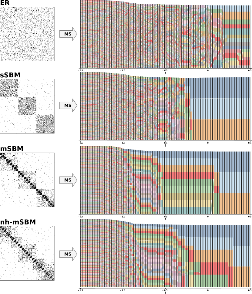
Figure 7: Sankey diagrams for multiscale clustering of synthetic data. The left column shows the adjacency matrices sampled from our four models (ER, sSBM, mSBM, nh-mSBM) as described above. Each adjacency matrix corresponds to a graph that is subsequently clustered with Markov Stability (MS) analysis into 200 partitions indexed by the Markov time $t$ equidistantly ranging from -1.5 to 0.5 and the obtained sequences of partitions are visualised with Sankey diagrams in the right column.

References

- [1] Mehmet E. Aktas, Esra Akbas and Ahmed El Fatmaoui “Persistence Homology of Networks: Methods and Applications” In Applied Network Science 4.1 SpringerOpen, 2019, pp. 1–28 URL: https://appliednetsci.springeropen.com/articles/10.1007/s41109-019-0179-3
- [2] M. Altuncu et al. “Extracting Information from Free Text through Unsupervised Graph-Based Clustering: An Application to Patient Incident Records”, 2019 arXiv: http://arxiv.org/abs/1909.00183
- [3] Alexis Arnaudon et al. “PyGenStability: Multiscale Community Detection with Generalized Markov Stability”, 2023 arXiv: http://arxiv.org/abs/2303.05385
- [4] Jean-Daniel Boissonnat “GUDHI Library”, 2022 URL: https://gudhi.inria.fr/index.html
- [5] Jean-Daniel Boissonnat, Tamal K. Dey and Clément Maria “The Compressed Annotation Matrix: An Efficient Data Structure for Computing Persistent Cohomology” In Algorithmica 73.3, 2015, pp. 607–619 URL: https://doi.org/10.1007/s00453-015-9999-4
- [6] Béla Bollobás “Random Graphs” Cambridge: Cambridge University Press, 2011
- [7] Kyle Brown “Topological Hierarchies and Decomposition: From Clustering to Persistence”, 2022 URL: https://etd.ohiolink.edu/apexprod/rws_olink/r/1501/10?clear=10&p10_accession_num=wright1650388451804736
- [8] Kyle Brown, Derek Doran, Ryan Kramer and Brad Reynolds “HELOC Applicant Risk Performance Evaluation by Topological Hierarchical Decomposition”, 2018 arXiv: http://arxiv.org/abs/1811.10658
- [9] Richard A. Brualdi “Introductory Combinatorics” Upper Saddle River, N.J: Pearson/Prentice Hall, 2010
- [10] Yueqi Cao and Anthea Monod “Approximating Persistent Homology for Large Datasets”, 2022 arXiv: http://arxiv.org/abs/2204.09155
- [11] Gunnar Carlsson “Topology and Data” In Bulletin of the American Mathematical Society 46.2, 2009, pp. 255–308 URL: https://www.ams.org/bull/2009-46-02/S0273-0979-09-01249-X/
- [12] Gunnar Carlsson and Facundo Mémoli “Characterization, Stability and Convergence of Hierarchical Clustering Methods” In Journal of Machine Learning Research 11.47, 2010, pp. 1425–1470 URL: http://jmlr.org/papers/v11/carlsson10a.html
- [13] Gunnar Carlsson, Facundo Mémoli, Alejandro Ribeiro and Santiago Segarra “Axiomatic Construction of Hierarchical Clustering in Asymmetric Networks” In 2013 IEEE International Conference on Acoustics, Speech and Signal Processing, 2013, pp. 5219–5223 DOI: 10.1109/ICASSP.2013.6638658
- [14] Joseph Minhow Chan, Gunnar Carlsson and Raul Rabadan “Topology of Viral Evolution” In Proceedings of the National Academy of Sciences 110.46, 2013, pp. 18566–18571 URL: https://pnas.org/doi/full/10.1073/pnas.1313480110
- [15] Frédéric Chazal and Steve Yann Oudot “Towards Persistence-Based Reconstruction in Euclidean Spaces” In Proceedings of the Twenty-Fourth Annual Symposium on Computational Geometry, SCG ’08 New York, NY, USA: Association for Computing Machinery, 2008, pp. 232–241 URL: https://doi.org/10.1145/1377676.1377719
- [16] Frédéric Chazal et al. “Gromov-Hausdorff Stable Signatures for Shapes Using Persistence” In Computer Graphics Forum 28.5, 2009, pp. 1393–1403 URL: https://onlinelibrary.wiley.com/doi/abs/10.1111/j.1467-8659.2009.01516.x
- [17] Frédéric Chazal, Vin Silva and Steve Oudot “Persistence Stability for Geometric Complexes” In Geometriae Dedicata 173.1, 2014, pp. 193–214 URL: http://link.springer.com/10.1007/s10711-013-9937-z
- [18] Jean-Charles Delvenne, Sophia N. Yaliraki and Mauricio Barahona “Stability of Graph Communities across Time Scales” In Proceedings of the National Academy of Sciences 107.29, 2010, pp. 12755–12760 URL: http://www.pnas.org/cgi/doi/10.1073/pnas.0903215107
- [19] Tamal K. Dey and Yusu Wang “Computational Topology for Data Analysis” New York: Cambridge University Press, 2022
- [20] Tamal K. Dey, Facundo Mémoli and Yusu Wang “Multiscale Mapper: Topological Summarization via Codomain Covers” In Proceedings of the Twenty-Seventh Annual ACM-SIAM Symposium on Discrete Algorithms Society for Industrial and Applied Mathematics, 2016, pp. 997–1013 URL: http://epubs.siam.org/doi/10.1137/1.9781611974331.ch71
- [21] Herbert Edelsbrunner and J. Harer “Computational Topology: An Introduction” Providence, R.I: American Mathematical Society, 2010
- [22] Herbert Edelsbrunner, David Letscher and Afra Zomorodian “Topological Persistence and Simplification” In Discrete & Computational Geometry 28.4, 2002, pp. 511–533 URL: https://doi.org/10.1007/s00454-002-2885-2
- [23] P Erdös and A Rényi “On Random Graphs I” In Publicationes Mathematicae Debrecen 6, 1959, pp. 290–297 DOI: 10.5486/PMD.1959.6.3-4.12
- [24] Renee S. Hoekzema et al. “Multiscale Methods for Signal Selection in Single-Cell Data” In Entropy 24.8 Multidisciplinary Digital Publishing Institute, 2022, pp. 1116 URL: https://www.mdpi.com/1099-4300/24/8/1116
- [25] Paul W. Holland, Kathryn Blackmond Laskey and Samuel Leinhardt “Stochastic Blockmodels: First Steps” In Social Networks 5.2, 1983, pp. 109–137 URL: https://www.sciencedirect.com/science/article/pii/0378873383900217
- [26] Danijela Horak, Slobodan Maletić and Milan Rajković “Persistent Homology of Complex Networks” In Journal of Statistical Mechanics: Theory and Experiment 2009.03, 2009, pp. P03034 URL: https://doi.org/10.1088/1742-5468/2009/03/p03034
- [27] A.. Jain, M.. Murty and P.. Flynn “Data Clustering: A Review” In ACM Computing Surveys 31.3, 1999, pp. 264–323 URL: https://doi.org/10.1145/331499.331504
- [28] Lida Kanari et al. “A Topological Representation of Branching Neuronal Morphologies” In Neuroinformatics 16.1, 2018, pp. 3–13 URL: https://doi.org/10.1007/s12021-017-9341-1
- [29] Lida Kanari, Adélie Garin and Kathryn Hess “From Trees to Barcodes and Back Again: Theoretical and Statistical Perspectives” In Algorithms 13.12 Multidisciplinary Digital Publishing Institute, 2020, pp. 335 URL: https://www.mdpi.com/1999-4893/13/12/335
- [30] Brian Karrer and M… Newman “Stochastic Blockmodels and Community Structure in Networks” In Physical Review E 83.1 American Physical Society, 2011, pp. 016107 URL: https://link.aps.org/doi/10.1103/PhysRevE.83.016107
- [31] Woojin Kim and Facundo Mémoli “Extracting Persistent Clusters in Dynamic Data via Möbius Inversion”, 2022 arXiv: http://arxiv.org/abs/1712.04064
- [32] Renaud Lambiotte, Jean-Charles Delvenne and Mauricio Barahona “Laplacian Dynamics and Multiscale Modular Structure in Networks”, 2009 arXiv: http://arxiv.org/abs/0812.1770
- [33] Renaud Lambiotte, Jean-Charles Delvenne and Mauricio Barahona “Random Walks, Markov Processes and the Multiscale Modular Organization of Complex Networks” In IEEE Transactions on Network Science and Engineering 1.2, 2014, pp. 76–90 URL: http://ieeexplore.ieee.org/document/7010026/
- [34] Ulrike Luxburg, Robert C. Williamson and Isabelle Guyon “Clustering: Science or Art?” In Proceedings of ICML Workshop on Unsupervised and Transfer Learning JMLR Workshop and Conference Proceedings, 2012, pp. 65–79 URL: https://proceedings.mlr.press/v27/luxburg12a.html
- [35] Jiří Matoušek “Using the Borsuk-Ulam Theorem: Lectures on Topological Methods in Combinatorics and Geometry”, Universitext Berlin ; New York: Springer, 2003
- [36] Nina Otter et al. “A Roadmap for the Computation of Persistent Homology” In EPJ Data Science 6.1, 2017, pp. 1–38 URL: https://epjdatascience.springeropen.com/articles/10.1140/epjds/s13688-017-0109-5
- [37] Tiago P. Peixoto “Hierarchical Block Structures and High-Resolution Model Selection in Large Networks” In Physical Review X 4.1 American Physical Society, 2014, pp. 011047 URL: https://link.aps.org/doi/10.1103/PhysRevX.4.011047
- [38] Michael T. Schaub, Jean-Charles Delvenne, Sophia N. Yaliraki and Mauricio Barahona “Markov Dynamics as a Zooming Lens for Multiscale Community Detection: Non Clique-Like Communities and the Field-of-View Limit” In PLoS ONE 7.2, 2012 URL: https://dx.plos.org/10.1371/journal.pone.0032210
- [39] Michael T. Schaub, Renaud Lambiotte and Mauricio Barahona “Encoding Dynamics for Multiscale Community Detection: Markov Time Sweeping for the Map Equation” In Physical Review E 86.2, 2012, pp. 026112 URL: https://link.aps.org/doi/10.1103/PhysRevE.86.026112
- [40] Michael T. Schaub, Jiaze Li and Leto Peel “Hierarchical Community Structure in Networks” In Physical Review E 107.5, 2023, pp. 054305 URL: https://link.aps.org/doi/10.1103/PhysRevE.107.054305
- [41] Dominik J. Schindler, Jonathan Clarke and Mauricio Barahona “Multiscale Mobility Patterns and the Restriction of Human Movement”, 2023 arXiv: http://arxiv.org/abs/2201.06323
- [42] Gurjeet Singh, Facundo Memoli and Gunnar Carlsson “Topological Methods for the Analysis of High Dimensional Data Sets and 3D Object Recognition” In Eurographics Symposium on Point-Based Graphics The Eurographics Association, 2007, pp. 10 pages URL: http://diglib.eg.org/handle/10.2312/SPBG.SPBG07.091-100
- [43] Primoz Skraba and Katharine Turner “Wasserstein Stability for Persistence Diagrams”, 2022 arXiv: http://arxiv.org/abs/2006.16824
- [44] Richard P. Stanley “Enumerative Combinatorics. Volume 1”, Cambridge Studies in Advanced Mathematics 49 Cambridge, NY: Cambridge University Press, 2011
- [45] Qingsong Wang “The Persistent Topology of Geometric Filtrations”, 2022 URL: https://etd.ohiolink.edu/apexprod/rws_olink/r/1501/10?p10_etd_subid=196459&clear=10
- [46] David Cheng Zarate et al. “Optimal Sankey Diagrams Via Integer Programming” In 2018 IEEE Pacific Visualization Symposium (PacificVis), 2018, pp. 135–139 DOI: 10.1109/PacificVis.2018.00025
- [47] Afra Zomorodian and Gunnar Carlsson “Computing Persistent Homology” In Discrete & Computational Geometry 33.2, 2005, pp. 249–274 URL: https://doi.org/10.1007/s00454-004-1146-y
- [48] Mehmet E. Aktas, Esra Akbas and Ahmed El Fatmaoui “Persistence Homology of Networks: Methods and Applications” In Applied Network Science 4.1 SpringerOpen, 2019, pp. 1–28 URL: https://appliednetsci.springeropen.com/articles/10.1007/s41109-019-0179-3
- [49] M. Altuncu et al. “Extracting Information from Free Text through Unsupervised Graph-Based Clustering: An Application to Patient Incident Records”, 2019 arXiv: http://arxiv.org/abs/1909.00183
- [50] Alexis Arnaudon et al. “PyGenStability: Multiscale Community Detection with Generalized Markov Stability”, 2023 arXiv: http://arxiv.org/abs/2303.05385
- [51] Jean-Daniel Boissonnat “GUDHI Library”, 2022 URL: https://gudhi.inria.fr/index.html
- [52] Jean-Daniel Boissonnat, Tamal K. Dey and Clément Maria “The Compressed Annotation Matrix: An Efficient Data Structure for Computing Persistent Cohomology” In Algorithmica 73.3, 2015, pp. 607–619 URL: https://doi.org/10.1007/s00453-015-9999-4
- [53] Béla Bollobás “Random Graphs” Cambridge: Cambridge University Press, 2011
- [54] Kyle Brown “Topological Hierarchies and Decomposition: From Clustering to Persistence”, 2022 URL: https://etd.ohiolink.edu/apexprod/rws_olink/r/1501/10?clear=10&p10_accession_num=wright1650388451804736
- [55] Kyle Brown, Derek Doran, Ryan Kramer and Brad Reynolds “HELOC Applicant Risk Performance Evaluation by Topological Hierarchical Decomposition”, 2018 arXiv: http://arxiv.org/abs/1811.10658
- [56] Richard A. Brualdi “Introductory Combinatorics” Upper Saddle River, N.J: Pearson/Prentice Hall, 2010
- [57] Yueqi Cao and Anthea Monod “Approximating Persistent Homology for Large Datasets”, 2022 arXiv: http://arxiv.org/abs/2204.09155
- [58] Gunnar Carlsson “Topology and Data” In Bulletin of the American Mathematical Society 46.2, 2009, pp. 255–308 URL: https://www.ams.org/bull/2009-46-02/S0273-0979-09-01249-X/
- [59] Gunnar Carlsson and Facundo Mémoli “Characterization, Stability and Convergence of Hierarchical Clustering Methods” In Journal of Machine Learning Research 11.47, 2010, pp. 1425–1470 URL: http://jmlr.org/papers/v11/carlsson10a.html
- [60] Gunnar Carlsson, Facundo Mémoli, Alejandro Ribeiro and Santiago Segarra “Axiomatic Construction of Hierarchical Clustering in Asymmetric Networks” In 2013 IEEE International Conference on Acoustics, Speech and Signal Processing, 2013, pp. 5219–5223 DOI: 10.1109/ICASSP.2013.6638658
- [61] Joseph Minhow Chan, Gunnar Carlsson and Raul Rabadan “Topology of Viral Evolution” In Proceedings of the National Academy of Sciences 110.46, 2013, pp. 18566–18571 URL: https://pnas.org/doi/full/10.1073/pnas.1313480110
- [62] Frédéric Chazal et al. “Gromov-Hausdorff Stable Signatures for Shapes Using Persistence” In Computer Graphics Forum 28.5, 2009, pp. 1393–1403 URL: https://onlinelibrary.wiley.com/doi/abs/10.1111/j.1467-8659.2009.01516.x
- [63] Frédéric Chazal, Vin Silva and Steve Oudot “Persistence Stability for Geometric Complexes” In Geometriae Dedicata 173.1, 2014, pp. 193–214 URL: http://link.springer.com/10.1007/s10711-013-9937-z
- [64] Frédéric Chazal and Steve Yann Oudot “Towards Persistence-Based Reconstruction in Euclidean Spaces” In Proceedings of the Twenty-Fourth Annual Symposium on Computational Geometry, SCG ’08 New York, NY, USA: Association for Computing Machinery, 2008, pp. 232–241 URL: https://doi.org/10.1145/1377676.1377719
- [65] Jean-Charles Delvenne, Sophia N. Yaliraki and Mauricio Barahona “Stability of Graph Communities across Time Scales” In Proceedings of the National Academy of Sciences 107.29, 2010, pp. 12755–12760 URL: http://www.pnas.org/cgi/doi/10.1073/pnas.0903215107
- [66] Tamal K. Dey, Facundo Mémoli and Yusu Wang “Multiscale Mapper: Topological Summarization via Codomain Covers” In Proceedings of the Twenty-Seventh Annual ACM-SIAM Symposium on Discrete Algorithms Society for Industrial and Applied Mathematics, 2016, pp. 997–1013 URL: http://epubs.siam.org/doi/10.1137/1.9781611974331.ch71
- [67] Tamal K. Dey and Yusu Wang “Computational Topology for Data Analysis” New York: Cambridge University Press, 2022
- [68] Herbert Edelsbrunner and J. Harer “Computational Topology: An Introduction” Providence, R.I: American Mathematical Society, 2010
- [69] Herbert Edelsbrunner, David Letscher and Afra Zomorodian “Topological Persistence and Simplification” In Discrete & Computational Geometry 28.4, 2002, pp. 511–533 URL: https://doi.org/10.1007/s00454-002-2885-2
- [70] P Erdös and A Rényi “On Random Graphs I” In Publicationes Mathematicae Debrecen 6, 1959, pp. 290–297 DOI: 10.5486/PMD.1959.6.3-4.12
- [71] Renee S. Hoekzema et al. “Multiscale Methods for Signal Selection in Single-Cell Data” In Entropy 24.8 Multidisciplinary Digital Publishing Institute, 2022, pp. 1116 URL: https://www.mdpi.com/1099-4300/24/8/1116
- [72] Paul W. Holland, Kathryn Blackmond Laskey and Samuel Leinhardt “Stochastic Blockmodels: First Steps” In Social Networks 5.2, 1983, pp. 109–137 URL: https://www.sciencedirect.com/science/article/pii/0378873383900217
- [73] Danijela Horak, Slobodan Maletić and Milan Rajković “Persistent Homology of Complex Networks” In Journal of Statistical Mechanics: Theory and Experiment 2009.03, 2009, pp. P03034 URL: https://doi.org/10.1088/1742-5468/2009/03/p03034
- [74] A.. Jain, M.. Murty and P.. Flynn “Data Clustering: A Review” In ACM Computing Surveys 31.3, 1999, pp. 264–323 URL: https://doi.org/10.1145/331499.331504
- [75] Lida Kanari et al. “A Topological Representation of Branching Neuronal Morphologies” In Neuroinformatics 16.1, 2018, pp. 3–13 URL: https://doi.org/10.1007/s12021-017-9341-1
- [76] Lida Kanari, Adélie Garin and Kathryn Hess “From Trees to Barcodes and Back Again: Theoretical and Statistical Perspectives” In Algorithms 13.12 Multidisciplinary Digital Publishing Institute, 2020, pp. 335 URL: https://www.mdpi.com/1999-4893/13/12/335
- [77] Brian Karrer and M… Newman “Stochastic Blockmodels and Community Structure in Networks” In Physical Review E 83.1 American Physical Society, 2011, pp. 016107 URL: https://link.aps.org/doi/10.1103/PhysRevE.83.016107
- [78] Woojin Kim and Facundo Mémoli “Extracting Persistent Clusters in Dynamic Data via Möbius Inversion”, 2022 arXiv: http://arxiv.org/abs/1712.04064
- [79] Renaud Lambiotte, Jean-Charles Delvenne and Mauricio Barahona “Laplacian Dynamics and Multiscale Modular Structure in Networks”, 2009 arXiv: http://arxiv.org/abs/0812.1770
- [80] Renaud Lambiotte, Jean-Charles Delvenne and Mauricio Barahona “Random Walks, Markov Processes and the Multiscale Modular Organization of Complex Networks” In IEEE Transactions on Network Science and Engineering 1.2, 2014, pp. 76–90 URL: http://ieeexplore.ieee.org/document/7010026/
- [81] Ulrike Luxburg, Robert C. Williamson and Isabelle Guyon “Clustering: Science or Art?” In Proceedings of ICML Workshop on Unsupervised and Transfer Learning JMLR Workshop and Conference Proceedings, 2012, pp. 65–79 URL: https://proceedings.mlr.press/v27/luxburg12a.html
- [82] Jiří Matoušek “Using the Borsuk-Ulam Theorem: Lectures on Topological Methods in Combinatorics and Geometry”, Universitext Berlin ; New York: Springer, 2003
- [83] Nina Otter et al. “A Roadmap for the Computation of Persistent Homology” In EPJ Data Science 6.1, 2017, pp. 1–38 URL: https://epjdatascience.springeropen.com/articles/10.1140/epjds/s13688-017-0109-5
- [84] Tiago P. Peixoto “Hierarchical Block Structures and High-Resolution Model Selection in Large Networks” In Physical Review X 4.1 American Physical Society, 2014, pp. 011047 URL: https://link.aps.org/doi/10.1103/PhysRevX.4.011047
- [85] Michael T. Schaub, Jean-Charles Delvenne, Sophia N. Yaliraki and Mauricio Barahona “Markov Dynamics as a Zooming Lens for Multiscale Community Detection: Non Clique-Like Communities and the Field-of-View Limit” In PLoS ONE 7.2, 2012 URL: https://dx.plos.org/10.1371/journal.pone.0032210
- [86] Michael T. Schaub, Renaud Lambiotte and Mauricio Barahona “Encoding Dynamics for Multiscale Community Detection: Markov Time Sweeping for the Map Equation” In Physical Review E 86.2, 2012, pp. 026112 URL: https://link.aps.org/doi/10.1103/PhysRevE.86.026112
- [87] Michael T. Schaub, Jiaze Li and Leto Peel “Hierarchical Community Structure in Networks” In Physical Review E 107.5, 2023, pp. 054305 URL: https://link.aps.org/doi/10.1103/PhysRevE.107.054305
- [88] Dominik J. Schindler, Jonathan Clarke and Mauricio Barahona “Multiscale Mobility Patterns and the Restriction of Human Movement”, 2023 arXiv: http://arxiv.org/abs/2201.06323
- [89] Gurjeet Singh, Facundo Memoli and Gunnar Carlsson “Topological Methods for the Analysis of High Dimensional Data Sets and 3D Object Recognition” In Eurographics Symposium on Point-Based Graphics The Eurographics Association, 2007, pp. 10 pages URL: http://diglib.eg.org/handle/10.2312/SPBG.SPBG07.091-100
- [90] Primoz Skraba and Katharine Turner “Wasserstein Stability for Persistence Diagrams”, 2022 arXiv: http://arxiv.org/abs/2006.16824
- [91] Richard P. Stanley “Enumerative Combinatorics. Volume 1”, Cambridge Studies in Advanced Mathematics 49 Cambridge, NY: Cambridge University Press, 2011
- [92] Qingsong Wang “The Persistent Topology of Geometric Filtrations”, 2022 URL: https://etd.ohiolink.edu/apexprod/rws_olink/r/1501/10?p10_etd_subid=196459&clear=10
- [93] David Cheng Zarate et al. “Optimal Sankey Diagrams Via Integer Programming” In 2018 IEEE Pacific Visualization Symposium (PacificVis), 2018, pp. 135–139 DOI: 10.1109/PacificVis.2018.00025
- [94] Afra Zomorodian and Gunnar Carlsson “Computing Persistent Homology” In Discrete & Computational Geometry 33.2, 2005, pp. 249–274 URL: https://doi.org/10.1007/s00454-004-1146-y