AdaptiveClick: Clicks-aware Transformer with Adaptive Focal Loss for Interactive
Image Segmentation

Abstract

Interactive Image Segmentation (IIS) has emerged as a promising technique for decreasing annotation time. Substantial progress has been made in pre- and post-processing for IIS, but the critical issue of interaction ambiguity notably hindering segmentation quality, has been under-researched. To address this, we introduce AdaptiveClick – a clicks-aware transformer incorporating an adaptive focal loss, which tackles annotation inconsistencies with tools for mask- and pixel-level ambiguity resolution. To the best of our knowledge, AdaptiveClick is the first transformer-based, mask-adaptive segmentation framework for IIS. The key ingredient of our method is the Clicks-aware Mask-adaptive Transformer Decoder (CAMD), which enhances the interaction between clicks and image features. Additionally, AdaptiveClick enables pixel-adaptive differentiation of hard and easy samples in the decision space, independent of their varying distributions. This is primarily achieved by optimizing a generalized Adaptive Focal Loss (AFL) with a theoretical guarantee, where two adaptive coefficients control the ratio of gradient values for hard and easy pixels. Our analysis reveals that the commonly used Focal and BCE losses can be considered special cases of the proposed AFL loss. With a plain ViT backbone, extensive experimental results on nine datasets demonstrate the superiority of AdaptiveClick compared to state-of-the-art methods. Code will be publicly available at https://github.com/lab206/AdaptiveClick.

I Introduction

Interactive Image Segmentation (IIS) tasks are designed to efficiently segment a reference object in an image by utilizing a minimal number of user operations, such as drawing boxes [1, 2, 3, 4], scribbling [5, 6], and clicking [7, 8, 9, 10]. Thanks to the unique interactivity and time-efficiency of this labeling paradigm, existing IIS models are widely used in fields such as medical image processing [11, 12, 13], 3D object segmentation [14, 15], and dataset production [8, 10, 16].

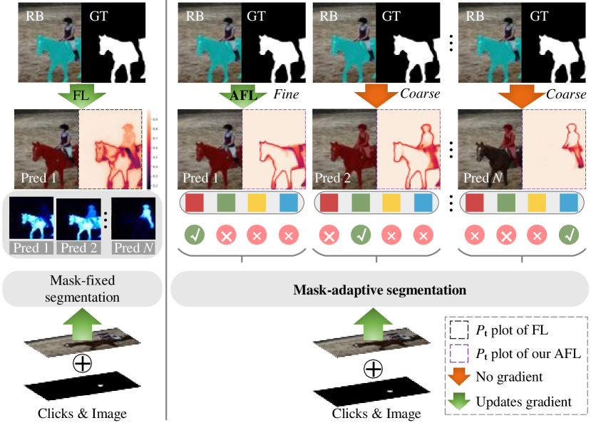
Figure 1: An illustration of the proposed method and the existing one. The left figure is the mask-fixed method, which only generates a single, fixed mask for each click. The right figure is the AdaptiveClick, which can generate multiple candidate masks (Pred $1\sim N$) for possible ambiguities of each click, and then select the optimal combination between the ground truth (GT) and prediction. Finally, the optimal combination is adaptively adjusted by using Adaptive Focal Loss (AFL) to output a higher-quality mask. The black and purple box is the $P_{t}$ plot of Focal loss (FL) and the AFL, respectively. Where $P_{t}$ is the confidence of the ease of each pixel in the sample, and the darker color means the pixel is more difficult to segment and vice versa.

A significant portion of interaction segmentation research targets clicks-based IIS. Existing studies explored clicks-based interactive image segmentation mainly from the perspective of data embedding [8, 17, 18], interaction ambiguity [19, 20, 21, 22], segmentation frameworks [23, 24], mask post-processing [23, 10], back-propagation [25, 26], and loss optimization [8, 9], which have effectively improved training convergence and stability, yielding impressive results. Although interaction ambiguity has been investigated in earlier studies [20, 21, 9], multiple deeper underlying issues have hindered effective solutions. These include: (1) inter-class click ambiguity: the problem of long-range propagation fading of clicks features and user click ambiguity, which leads to unclear semantic representation and (2) intra-class click ambiguity: the problem of low-confidence pixels (ambiguous pixels) not being correctly classified due to gradient swamping. On the one hand, the existing transformer-based IIS models predominantly rely on a mask-fixed segmentation strategy. This approach entails generating a single, fixed mask for each click during a training loop, as depicted on the left side in Fig. 1). On the other hand, focal loss-based optimization, which is widely used in IIS tasks, has the risk of “gradient swamping”, particularly evident for vision transformers. “Gradient swamping” refers to the phenomenon of focal loss focusing too much on the classification of hard pixels, significantly weakening the gradient values that many low-confidence easy pixels should contribute. As shown in the $P_{t}$ plot of the black box in the left subfigure of Fig. 1, this weakening can lead to the misclassification of ambiguous pixels and exacerbate problems with interaction ambiguity.

In this paper, we rethink interactive image segmentation by looking at the inter-class click ambiguity resolution and intra-class click ambiguity optimization (refer to the right-hand figure in Fig. 1) and propose an AdaptiveClick model, which is a clicks-aware transformer with an adaptive focal loss. First, we develop a click-aware mask-adaptive transformer decoder (CAMD) that includes a Pixel-level Multi-scale Mask Transformer Decoder (PMMD) and a Clicks-Aware Attention Module (CAAM). This decoder generates unique instance masks for each ambiguity based on possible click ambiguities and selects the optimal mask based on the ground truth. This approach resolves interaction ambiguity and accelerates the convergence of the transformer. Then, we investigate the “gradient swamping” problem of focal loss, which aggravates interaction ambiguity in IIS tasks. To tackle this, we design a novel Adaptive Focal Loss (AFL). AFL adapts the training strategy according to the number and difficulty distribution of samples, improving convergence and interaction ambiguity problems (see the $P_{t}$ plot purple box in the right sub-figure in Fig. 1). At a glance, the main contributions delivered in this work are summarized as follows:

1) A novel mask-adaptive segmentation framework is designed for IIS tasks. To the best of our knowledge, this is the first mask-adaptive segmentation framework based on transformers in the context of IIS;

2) We designed a new clicks-aware attention module and a clicks-aware mask-adaptive transformer decoder to tackle the problem of interaction ambiguity arising from user ambiguity clicks and the long-range propagation fading of clicks features in the IIS model;

3) A novel adaptive focal loss is designed to overcome the “gradient swamping” problem of specific to focal loss-based training in IIS, which accelerates model convergence and alleviates the interaction ambiguity;

4) Experimental results from nine benchmark datasets showcase clear benefits of the proposed AdaptiveClick method and adaptive focal loss, yielding performance that is better or comparable to state-of-the-art IIS methods.

The remainder of the paper is structured as follows: Sec. II provides a brief overview of related work. The proposed methods are presented in Sec. III. We present experimental results in Sec. IV, followed by the conclusion in Sec. VI.

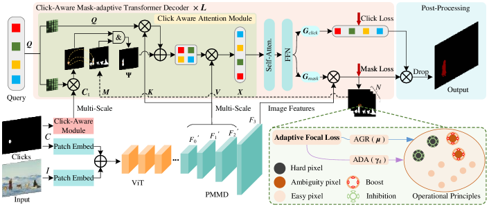
Figure 2: An illustration of the proposed AdaptiveClick. First, clicks ($C$) and image ($I$) are obtained via patch embedding to encode features $C_{t}$ and $I_{t}$, then fused together by an addition operation. Second, the fusion features are obtained by an encoder backbone, and the pixel features $F_{0}$, $F_{1}$, and $F_{2}$ of different dimensions are obtained by the designed Pixel-level Multi-scale Mask Transformer Decoder (PMMD). Third, $F^{{}^{\prime}}_{0},F^{{}^{\prime}}_{1},F^{{}^{\prime}}_{2}$, and $F_{3}$ and clicks are jointly input into the designed Click-aware Mask-adaptive Transformer Decoder (CAMD). Fourth, the model generates $N$ corresponding masks $\hat{p}$ based on each click and then completes the optimization training process with ADA and AGR proposed in Adaptive Focal Loss (AFL). Finally, the obtained mask sequences are passed through the post-processing to output the final mask $P_{n}$.

II Related Work

II-A Architecture of Interactive Image Segmentation

In the IIS task, the goal is to obtain refined masks by effectively leveraging robust fusion features activated by click information. Interaction strategies in mainstream research works can be generally divided into three categories: pre-fusion [27, 17, 8, 28], secondary fusion [16, 17, 19, 29] and middle fusion [30, 31, 32, 33].

Pre-fusion methods incorporate clicks information as an auxiliary input, which includes click features [27] or additional previous masks [8, 10, 28]. Starting with clicks embedding via distance transformation in [27], a common technique is to concatenate maps of clicks with raw input [25, 20, 34]. Subsequently, Benenson et al. [35] suggest that, using clicks with an appropriate radius offers better performance. Nevertheless, due to the potential absence of pure interaction strategies in [27], another line of work [36, 8] constructively employs masks predicted from previous clicks as input for subsequent processing. Following this simple yet effective strategy, several studies have achieved remarkable results, such as incorporating cropped focus views [37] or exploiting visual transformers[38] as the backbone [28]. Although the above methods strive to maximize the use of click information, the click feature tends to fade during propagation, exacerbating interaction ambiguity and leading to suboptimal model performance.

To address the aforementioned issues, secondary fusion has been introduced as a potential solution. Building upon strategies in [27], some previous works focused on alleviating the interaction ambiguity problem. Examples include emphasizing the impact of the first clicks [17], long-range propagation strategy for clicks [19], and utilizing multi-scale strategies [21]. Inspired by the success of [8], Chen et al. [23] further fuse clicks and previous masks for the refinement of local masks. Recently, drawing from [8], Wei et al. [29] proposed a deep feedback-integrated strategy that fuses coordinate features with high-level features. Moreover, other recent works [25, 26, 39] have combined click-embedding strategies [27] with an online optimization approach. These methods are designed to eventually boost the accuracy via pre-fusion strategies. However, no existing research has explored overcoming the challenge of interaction ambiguity in vision transformers.

Recently, middle fusion strategies have gained popularity in the IIS field. Unlike pre-fusion methods, these strategies do not directly concatenate click information with raw input. Kirillov et al. [30] propose a novel strategy that treats clicks as prompts [40], supporting multiple inputs. Similarly, Zou et al. [33] concurrently suggest joint prompts for increased versatility. For better efficiency, Huang et al. [31] bypass the strategies in [8] related to the backbone to perform inference multiple times. Inspired by Mask2Former [41], a parallel study [32] models click information as queries with the timestamp to support multi-instance IIS tasks. Although these models achieve remarkable success in more challenging tasks, they sacrifice the performance of a single IIS task to enhance the multi-task generalization.

In this paper, we first explore vision transformers for IIS tasks, focusing on mask-adaptive click ambiguity resolution. Specifically, we achieve long-range click propagation within transformers through a click-aware attention module. At the same time, mask-adaptive segmentation generates $N$ candidate masks from ambiguity clicks and selects the optimal one for the final inference, breaking the limitations of the existing mask-fixed models.

Works most similar to ours are presumably SimpleClick [28] and DynaMITe [32]. While these works, similarly to ours, implement models based on vision transformers, the main difference lies in the fact that both [28] and [32] utilize mask-fixed models, whereas the key ingredient of our model is the inter-class click ambiguity resolution (CAMD) approach. Furthermore, both SimpleClick and DynaMITe suffer from interaction ambiguity issues caused by gradient swamping. To address this limitation, this paper introduces a novel intra-class click ambiguity optimization (AFL) technique that effectively resolves the interaction ambiguity problems found in the aforementioned models.

II-B Loss Function of Interactive Image Segmentation

The Binary Cross Entropy (BCE) loss [42] and its variants [37, 43, 44, 45, 46] are widely used in object detection and image segmentation. In the context of IIS tasks, early works, such as  [25, 21, 47, 48], typically utilize BCE for training. However, BCE treats all pixels equally, resulting in a gradient of easy pixels inundated by hard pixels and blocking the models’ performance. Previous works [37, 43, 44] attempt to solve this problem from two perspectives: the imbalance of positive and negative samples [44, 45, 49, 50] or the easy sample and hard sample [37, 43].

To counteract the imbalance between positive and negative samples, the WBCE loss [44], a loss function based on BCE, introduces a weighting coefficient for positive samples. Furthermore, the balanced CE loss [45] weights not only positive samples but also negative samples. These functions are used with data that satisfies a skewed distribution [51] but are blocked in balanced datasets due to their adjustable parameters, which influence the model’s performance.

To address the imbalance between hard and easy samples, the Focal Loss (FL) [37] formulates a modulating factor to enhance model training and down-weight the impact of easy examples, thereby allowing the model to concentrate more on the challenging examples. In recent works, Leng et al. [43] offer a new perspective on loss function design and propose the Poly Loss (PL) as a linear combination of polynomial functions. In the IIS field, Sofiiuk et al. [52] present the Normalized Focal Loss (NFL) which expands an extra correction factor negatively correlated with the total modulate factor in FL. In addition, some other works [49, 50] also attempt to solve this problem. However, deeper reasons, such as the case that many low-confidence samples are caused by gradient swamping, make it easy that some samples of ambiguous samples cannot to be effectively classified.

In brief, it is crucial for the IIS tasks to address the issue of “gradient swamping” for FL-based losses. Unlike previous works [25, 26], we consider the interaction ambiguity problem prevalent in IIS tasks from the perspective of the intra-class click ambiguity optimization level. Therefore, in this work, the model can focus more on low-confidence easy pixels (ambiguous pixels) for IIS tasks than simply computing gradient values point by point equally during the gradient backpropagation process.

III Method

At a high level, AdaptiveClick’s primary components consist of four key stages: (1) data embedding, (2) feature encoding, (3) feature decoding, and (4) loss optimization. These stages are illustrated and summarized in Fig. 2. In our approach, we address the interaction ambiguity by focusing on the aspects of feature decoding and loss optimization.

III-A Deficiency of Existing IIS Methods

We begin by discussing common challenges faced by modern interactive segmentation models, which motivated our proposed methodology. In this paper, we categorize interaction ambiguity into inter-class and intra-class interaction ambiguity. Inter-class interaction ambiguity refers to the problem of unclear semantic referencing caused by click ambiguity or clicks during long-range propagation. Intra-class ambiguity refers to the problem that the model cannot be correctly classified due to the hard, ambiguous, and pixel-prone referencing of the object region stemming from the gradient swamping phenomenon.

This paper tackles both, the inter-class and intra-class ambiguity problems, by focusing on two distinct aspects: resolving inter-class click ambiguity and optimizing intra-class click ambiguity, respectively.

Inter-class Click Ambiguity Resolution. Some studies have preliminary explored interaction ambiguity in the direction of multi-scale transformation [20, 21, 9] and click long-range propagation [19, 17, 22]. However, all these studies consider the interaction ambiguity problem from the click enhancement perspective. Although these methods can effectively improve the guiding role of clicks in the segmentation process, they still require tools for effectively dealing with click ambiguity. Therefore, such methods can only make the model generate ground truth-compliant masks as much as possible by enhancing the clicks.

Intra-class Click Ambiguity Optimization. Given the prediction $P_{n}$ and its corresponding ground truth ($y_{t}$), the Binary Cross-Entropy (BCE) loss [42] widely applied in recent works [8, 25, 10] can be expressed as,

$$\mathbb{\ell}_{\mathrm{bce}}=-\sum_{i=1}^{\mathcal{N}}\mathrm{log}(P^{i}_{t}).$$ (1)

where $P^{i}_{t}\in[0,1]$ is the value reflecting the confidence level of the difficulty of the pixel in the sample, $P^{i}_{t}=\left\{\begin{matrix}P^{i}_{n},\mathrm{if}\indent y^{i}_{t}=1\\ 1-P^{i}_{n},\mathrm{else}\indent y^{i}_{t}=0\end{matrix}\right.$, $P^{i}_{n}\in P_{n}$, $P^{i}_{t}\in P_{t}$ and $y^{i}_{t}\in y_{t}$, the $H$ and $W$ are the height, width of the $P_{n}$, and $\mathcal{N}=HW$.

However, $\mathbb{\ell}_{\mathrm{bce}}$ treats hard and easy pixels equally [37], we call this property of BCE “Difficulty-equal” (A theoretical proof will be obtained in Eq. (13)), which will result in many hard pixels not being effectively segmented. To solve the problems of $\mathbb{\ell}_{\mathrm{bce}}$, Focal Loss $\mathbb{\ell}_{\mathrm{fl}}$ [37] is introduced in recent IIS works [28, 53, 31, 32]. The $\mathbb{\ell}_{\mathrm{fl}}$ can be defined as:

$$\mathbb{\ell}_{\mathrm{fl}}=-\sum_{i=1}^{\mathcal{N}}(1-P^{i}_{t})^{\gamma}\mathrm{log}(P^{i}_{t}).$$ (2)

where $(1-P^{i}_{t})^{\gamma}$ is the difficulty modifier, $\gamma\in[0,5]$, the larger the $\gamma$, the greater the weight for hard pixels. $\mathbb{\ell}_{\mathrm{fl}}$ can solve the imbalance of hard and easy pixels in the IIS task more effectively compared to $\mathbb{\ell}_{\mathrm{bce}}$ due to it “Difficulty-oriented” property (a theoretical proof will be obtained in Eq. (14)).

However, one study [43] points out that the coefficients of each Taylor term in Eq. (2) are not optimal, so the poly loss was proposed as a correction scheme to improve the performance of $\mathbb{\ell}_{\mathrm{fl}}$. The poly loss $\mathbb{\ell}_{\mathrm{pl}}$ can be expressed as

$$\mathbb{\ell}_{\mathrm{pl}}=-\sum_{i=1}^{\mathcal{N}}\left[(1-P^{i}_{t})^{\gamma}\mathrm{log}(P^{i}_{t})+\alpha(1-P^{i}_{t})^{\gamma+1}\right].$$ (3)

where the $\alpha$ is a coefficient of $\mathbb{\ell}_{\mathrm{pl}}$.

Such an improvement is beneficial, but as shown in Fig. 3, we observe that pixels around the click target boundaries (for example, the person next to the lady in white in the second row) are still difficult to classify correctly. We define such pixels as low-confidence easy pixels or ambiguous pixels in the IIS task. This phenomenon occurs because both BCE [42] and FL [37] suffer from the gradient swamping problem. The difference is that, due to the “Difficulty-equal” property, the gradient swamping of BCE is mainly the result of a large number of easy pixels swamping the gradients of hard pixels. In contrast, due to the stiff “Difficulty-oriented” property, the gradient swamping problem of FL comes from the gradients of the low-confidence easy pixels being swamped by the hard pixels. Such a dilemma prevents ambiguous pixels from achieving excellent performance and even aggravates the interaction ambiguity problem of the IIS model. We consider this phenomenon as “Gradient swamping by FL-based loss of ambiguous pixels in IIS”.

III-B Inter-class Click Ambiguity Resolution

Previous studies [8, 28] have experimented with using prior clicks as a prior knowledge input into the model to help it converge faster and focus more precisely on local features. Motivated by this, we rethink the defects of mask-fixed strategy in the existing IIS model and look at them through the lens of interaction ambiguity. Unlike prior works, AdaptiveClick considers the problem of clicks-aware localization and mask-adaptive segmentation. Taking the above two limitations as a breakthrough, we explore a mask-adaptive IIS segmentation to solve the interaction ambiguity.

III-B1 Pixel-level Multi-scale Mask Transformer Decoder

To obtain representations with more subtle feature differences of different clicks, we expand the fusion features $F$ to $1/8$, $1/16$, and $1/32$ resolution based on the Feature Pyramid Networks (FPN) [54]. Then, $F_{0}$, $F_{1}$, and $F_{2}$ are passed to the decoder, which has $6$ multi-scale deformable attention transformer layers proposed in [55], to obtain $F^{{}^{\prime}}_{0}$, $F^{{}^{\prime}}_{1}$, and $F^{{}^{\prime}}_{2}$, respectively. Finally, a simple lateral up-sampling layer is used on the $1/8$ feature map to generate a feature map $F_{3}$ with a resolution of $1/4$ as a pixel-by-pixel embedding.

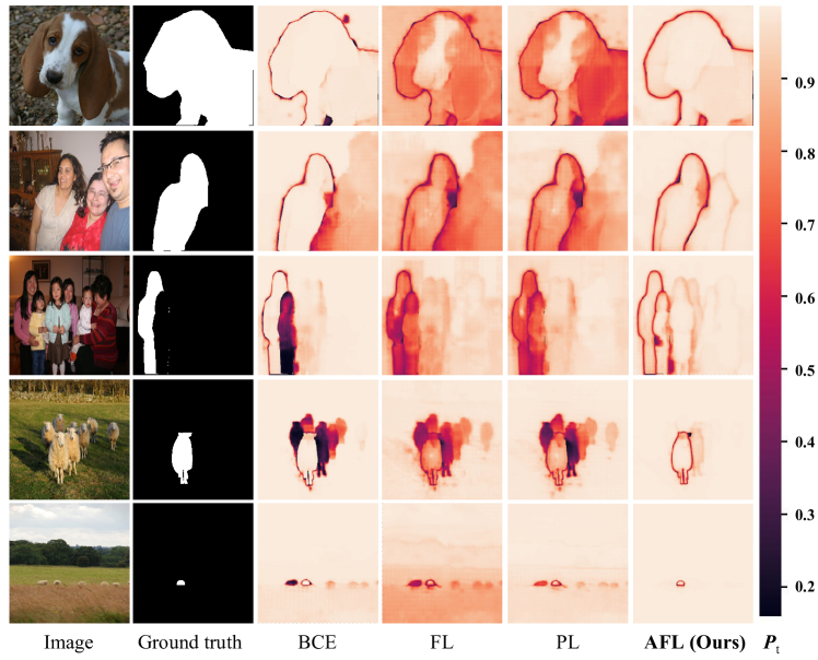
Figure 3: Difficulty confidence visualization of different loss functions on the SBD [18] training dataset in the IIS task. From left to right are the original image, the ground truth, and the $P_{t}$ plot of BCE [42], FL [37], PL [43], and proposed AFL, respectively.

III-B2 Click-Aware Mask-adaptive Transformer Decoder

The proposed Clicks-Aware Mask-adaptive Transformer Decoder (CAMD) primarily consists of the Clicks-aware Attention Module (CAAM), self-attention module [41, 56], feed-forward network, and the clicks- and mask prediction head.

Clicks-aware Attention Module. Given a set of clicks $\left\{C^{1}_{t},C^{2}_{t},C^{3}_{t}\right\}$ and their corresponding different scales decoding features $\left\{F^{{}^{\prime}}_{0},F^{{}^{\prime}}_{1},F^{{}^{\prime}}_{2}\right\}$, the attention matrix of the proposed CAAM can be expressed as,

$$X_{\mathrm{l}}=\mathrm{softmax}(\Psi_{l-1}+Q_{l}K^{\mathsf{T}}_{l}V_{l})+X_{l-1},$$ (4)

where $l$ is the layer index value, $X_{l}\in\mathrm{R}^{N\times d}$ is the $N\times d$-dimensional query feature of the $l$-th layer, and $Q_{l}=f_{Q}(X_{l-1})\in\mathrm{R}^{N\times d}$. $X_{0}$ denotes the input query feature of the transformer decoder. $K_{l}$, $V_{l}\in\mathrm{R}^{H_{l}W_{l}\times d}$ are the image features under the transformations $f_{k}$ and $f_{v}(*)$ from $\left\{F^{{}^{\prime}}_{0},F^{{}^{\prime}}_{1},F^{{}^{\prime}}_{2}\right\}$, respectively, and $H_{l}$ and $W_{l}$ are the spatial resolutions of the $\left\{F^{{}^{\prime}}_{0},F^{{}^{\prime}}_{1},F^{{}^{\prime}}_{2}\right\}$. $f_{Q}$, $f_{k}$ and $f_{v}$ are linear transformations. $\Psi_{l-1}$ denotes the click attention matrix.

The $\Psi_{l-1}$ attention matrix can be obtained via Eq. (5)

$$\Psi_{l-1}=\psi[\omega_{f}(C^{{}^{\prime}}_{t})[Q_{l}]_{+}^{\mathsf{T}}]\&\mathbb{M}_{l-1},$$ (5)

where $\omega_{f}$ is the click-aware module, which consists of a max pooling layer and a single linear layer. $\psi$ denotes the linear mapping layer, $[*]_{+}$ represents the max function, $\&$ represents the $and$ operation, and $C^{{}^{\prime}}_{t}\in\left\{C^{1}_{t},C^{2}_{t},C^{3}_{t}\right\}$. $\Psi_{0}$ is the binary click prediction obtained from $X_{0}$, i.e., before the query features being fed to the transformer decoder. $\mathbb{M}_{l-1}$ represents the attention mask of the previous transformer block, which can be calculated by Eq. (6)

$$\mathbb{M}_{l-1}(i,j)=\left\{\begin{matrix}0,\indent\mathrm{if}\indent F_{3}(\hat{p}_{\small l-1})^{\mathsf{T}}(i,j)=1\\ -\infty,\indent\mathrm{otherwise}\end{matrix}\right.,$$ (6)

where $F_{3}(\hat{p}_{\small l-1})^{\mathsf{T}}\in[0,1]^{N\times H_{l}W_{l}}$ is the binarized output of the mask prediction resized by the previous $l-1$-th transformer decoder layer (with a threshold of $0.5$).

Mask Prediction Head. We define mask prediction head as $G_{mask}$, which consists of three MLP layers of shape $N\times d$. $G_{mask}$ takes predicted object query $Q_{l}$ as input and outputs a click-based prediction mask $\hat{p_{i}}=G_{mask}(Q_{l})$.

Clicks Prediction Head. To allow our model to produce click predictions, we proposed a clicks prediction head $G_{click}$, which consists of a single linear layer of shape $N\times 2$ followed by a softmax layer. Given a $Q_{l}\in\mathrm{R}^{d}$, $G_{click}$ takes $Q_{l}$ as input and outputs a click prediction $\hat{c}=G_{click}(Q_{l})$.

III-B3 Mask-adaptive Matching Strategy

To discriminate and generate a perfect mask without ambiguity, we use the Hungarian algorithm similar to [41, 57, 58] to find the optimal permutation $\hat{\mathbb{\sigma}}$ generated between the $P_{n}$ and the $y_{t}$ during the mask-adaptive optimization process, and finally to optimize the object target-specific losses. Accordingly, we search for a permutation $\hat{\mathbb{\sigma}}\in S_{N_{q}}$ with the lowest total cost,

$$\hat{\mathbb{\sigma}}=\underset{\sigma\in S_{N_{q}}}{\mathrm{argmin}}\sum_{i=1}^{N_{q}}\mathbb{L}_{\mathrm{Match}}(\hat{p}\mathbb{\sigma}(i),y^{i}_{p}).$$ (7)

where the $\hat{p}$ is the set of the predicted via clicks instance and $\hat{p}=\left\{\hat{p_{i}}\right\}_{i=1}^{N_{q}}$. $N_{q}$ is the number of predicted via clicks instances. Similarly, $y^{i}_{p}$ is the set of the ground truth via clicks instance. Where each $\hat{p_{i}}$ and $y^{i}_{p}$ can be obtained from $\hat{p_{i}}=(\hat{p_{i}},c_{i})$ and $y^{i}_{p}=(y^{i}_{t},c_{i})$, respectively. where the $y^{i}_{t}$ is a ground truth mask, and $c_{i}\in\left\{0,1\right\}^{2}$ is a one hot click vector.

Inspired by [41, 57], CAMD uses an efficient multi-scale strategy to exploit high-resolution features. It feeds continuous feature mappings from the PMMD to the continuous CAMD in a cyclic manner. It is worth mentioning that the CAMD enables clicks to propagate over a long range and accelerates the model’s convergence. This is because, in previous works [41, 57, 58], the optimization of the query had a random property. However, CAMD can correctly pass the clicks to the fine mask in $\hat{p}$, thus achieving the convergence of the model faster while using clicks to guide the model to locate the objects effectively.

III-C Intra-class Click Ambiguity Optimization

There are no studies focused on solving the gradient swamping problem in image segmentation. Similar studies only explored the imbalance problem for positive and negative pixels [44, 45], and the imbalance problem for hard and easy pixels [37, 52, 43] of BCE loss. Unlike these works [8, 52, 37, 43], we rethink the gradient swamping of FL and propose a global-local-pixel computation strategy from the perspective of sample guidance pixel optimization based on the gradient theory of BCE and FL. It enables the model to adapt the learning strategy according to the global training situation, effectively mitigating the gradient swamping problem.

III-C1 Adaptive Difficulty Adjustment (ADA)

Observing Eqs. (2) and (3), $\mathbb{\ell}_{\mathrm{fl}}$ and $\mathbb{\ell}_{\mathrm{pl}}$ uses $(1-P^{i}_{t})^{\gamma}$ as the difficulty modifier, and adjusts the value of $(1-P^{i}_{t})^{\gamma}$ using initial $\gamma$ according to the difficulty distribution of the dataset empirically (i.e., generally taken as $2$ in previous works). However, it is worth noting that the distribution of difficulty varies among samples even in the same dataset (see Fig. 3). Therefore, giving a fixed $\gamma$ to all training samples of a dataset is a suboptimal option.

To give the model the ability to adaptively adjust $(1-P^{i}_{t})^{\gamma}$ according to the different difficulty distributions of the samples and different learning levels, we introduce an adaptive difficulty adjustment factor $\gamma_{a}$. The $\gamma_{a}$ can adjust $(1-P^{i}_{t})^{\gamma}$ of each pixel according to the overall training of the samples, giving the model the capability of “global insight”.

Given $I$, we refer to the foreground as the hard pixels and the number as $\mathcal{H}$ (obtained through $y_{t}$). To estimate the overall learning difficulty of the model, we use the $P^{i}_{t}$ of each pixel to represent its learning level. Then, the learning state of the model can be denoted as $\sum_{i=1}^{\mathcal{H}}(P^{i}_{t})$. Ideally, the optimization goal of the model is to classify all hard pixels completely and accurately. In this case, the optimal learning situation of the model can be represented as $\sum_{i=1}^{\mathcal{H}}(y^{i}_{t})$. As a result, the actual learning situation of the model can be represented as $\tiny{\frac{\sum_{i=1}^{\mathcal{H}}(P^{i}_{t})}{\sum_{i=1}^{\mathcal{H}}(y^{i}_{t})}}$. Given the FL properties, $\mathbb{\gamma}_{\mathrm{a}}$ can be represented as

$$\mathbb{\gamma}_{\mathrm{a}} =1-\frac{\sum_{i=1}^{\mathcal{H}}(P^{i}_{t})}{\sum_{i=1}^{\mathcal{H}}(y^{i}_{t})},$$ (8)

Then, the new difficulty modifier can be expressed as $(1-P_{t})^{\gamma_{\mathrm{d}}}$, where

$$\gamma_{\mathrm{d}}=\gamma+\gamma_{\mathrm{a}},$$ (9)

In summary, the AFL can be expressed as:

$$\mathbb{\ell}_{\mathrm{afl}} =\sum_{i=1}^{\mathcal{N}}-(1-P^{i}_{t})^{\gamma_{\mathrm{d}}}\mathrm{log}(P^{i}_{t})+\alpha(1-P^{i}_{t})^{\gamma_{\mathrm{d}}+1}.$$ (10)

III-C2 Adaptive Gradient Representation (AGR)

For IIS tasks, a larger $\gamma_{\mathrm{d}}$ is suitable when a more severe hard-easy imbalance is present. However, for the same $P_{t}$, the larger of $\gamma_{\mathrm{d}}$, the smaller the loss. It leads to the fact that when one wants to increase the concentration on learning with severe hard-easy imbalance, it tends to sacrifice a portion of low-confidence easy pixels’ loss in the overall training process. Although ADA can somewhat alleviate this gradient swamping, it provides only a partial solution.

At first, we explored the gradient composition of $\mathbb{\ell}_{\mathrm{afl}}$ and its properties based on Taylor approximation theory [59] of Eq. (1), we can obtain Eq. (12),

$$\mathbb{\ell}_{\mathrm{bce}} =\sum_{i=1}^{\mathcal{N}}\left[(1-P^{i}_{t})+\frac{1}{2}(1-P^{i}_{t})^{2}+...\right],$$ (11)

To further explore the theoretical connection between the $\mathbb{\ell}_{\mathrm{bce}}$ and proposed $\mathbb{\ell}_{\mathrm{afl}}$, we conducted an in-depth study at the gradient level of Eq. (10) and obtain

$$\mathbb{\ell}_{\mathrm{afl}} =\sum_{i=1}^{\mathcal{N}}\left[(1+\alpha)(1-P^{i}_{t})^{\gamma_{\mathrm{d}}+1}+\frac{1}{2}(1-P^{i}_{t})^{\gamma_{\mathrm{d}}+2}+...\right],$$ (12)

Next, we derive Eq. (11) of $\mathbb{\ell}_{\mathrm{bce}}$, which yields:

$$-\frac{\partial\mathbb{\ell}_{\mathrm{bce}}}{\partial P_{t}} =-\sum_{i=1}^{\mathcal{N}}\nu_{i}=\sum_{i=1}^{\mathcal{N}}\left[1+(1-P^{i}_{t})^{1}+(1-P^{i}_{t})^{2}+...\right],$$ (13)

Where $\nu_{i}=\tfrac{\partial\mathbb{\ell}_{\mathrm{bce}}}{\partial P^{i}_{t}}$ is the gradient of BCE for each pixel in the sample. The first term of the $\nu_{i}$ in Eq. (13) is always $1$, regardless of the difficulty of the pixel, which indicates that the gradient of $\mathbb{\ell}_{\mathrm{bce}}$ is “Difficulty-equal”, treating all pixels equally. Because of this property, $\mathbb{\ell}_{\mathrm{bce}}$ can perform competitively in pixels with uniform difficulty distribution, but often performs poorly when the difficulty pixels are imbalanced (See Fig. 3, the visualization of BCE [42]).

Interestingly, when deriving Eq. (12) of proposed $\mathbb{\ell}_{\mathrm{afl}}$, we can obtain,

$$-\frac{\partial\mathbb{\ell}_{\mathrm{afl}}}{\partial P_{t}} =\!\!\sum_{i=1}^{\mathcal{N}}(1-P^{i}_{t})^{\gamma_{\mathrm{d}}}\left[(1+\alpha)(1+\gamma_{\mathrm{d}})\!+\!(1+\frac{\gamma_{\mathrm{d}}}{2})(1-P^{i}_{t})\!+\!...\right],$$ (14)

In contrast to $\mathbb{\ell}_{\mathrm{bce}}$, the gradient of $\mathbb{\ell}_{\mathrm{afl}}$ is “Difficulty-oriented”, and the values of all gradient terms vary with the difficulty of the sample. Due to the “Difficulty-oriented” property, the gradient swamping problem of $\mathbb{\ell}_{\mathrm{afl}}$ comes from the gradients of the ambiguous pixels being swamped by the hard pixels.

In view of the above analysis, we expect that the proposed $\mathbb{\ell}_{\mathrm{afl}}$ can have the ability of $\mathbb{\ell}_{\mathrm{fl}}$ to classify hard and easy pixels while taking into account the focus on ambiguous pixels like $\mathbb{\ell}_{\mathrm{bce}}$. Observing Eq. (13) and Eq. (14), we can see that the gradient value of $\mathbb{\ell}_{\mathrm{afl}}$ can be approximated as the value of $\mathbb{\ell}_{\mathrm{bce}}$ gradient discarding the first $\gamma_{\mathrm{d}}$ terms. Therefore, the gradient value of $\mathbb{\ell}_{\mathrm{afl}}$ can be represented by $\mathbb{\ell}_{\mathrm{bce}}$. There are two ways to make the $\mathbb{\ell}_{\mathrm{afl}}$’s gradient approximate to $\mathbb{\ell}_{\mathrm{bce}}$: (1) adding two gradients that approximate $\mathbb{\ell}_{\mathrm{bce}}$ to $\mathbb{\ell}_{\mathrm{afl}}$, making the $\mathbb{\ell}_{\mathrm{afl}}$’s gradient similar to $\mathbb{\ell}_{\mathrm{bce}}$; (2) multiplying by an adaptive gradient representation factor that forces the $\mathbb{\ell}_{\mathrm{afl}}$’s gradient to infinitely approximate to total $\mathbb{\ell}_{\mathrm{bce}}$.

Unfortunately, the first option is not feasible in practice. The main reason is that adding the missing terms $\sum_{i=1}^{\mathcal{N}}\sum_{j=1}^{\gamma_{\mathrm{d}}}(1-P^{i}_{t})^{j+1}$ in Eq. (14) still introduces the “Difficulty-equal” properties of $\mathbb{\ell}_{\mathrm{bce}}$. Therefore, we mainly explore the second gradient approximation scheme.

Based on this conjecture, we summarized the gradient of $\mathbb{\ell}_{\mathrm{bce}}$ to that of $\mathbb{\ell}_{\mathrm{afl}}$ at the gradient level. Then, we find that the adjustment of $\mathbb{\ell}_{\mathrm{afl}}$ to the $\mathbb{\ell}_{\mathrm{bce}}$ is mainly focused on the vertical direction of the gradient, e.g., in Eq. (15),

$$-\frac{\partial\mathbb{\ell}_{\mathrm{afl}}}{\partial P_{t}}=\sum_{i=1}^{\mathcal{N}}(1-P^{i}_{t})^{\gamma_{\mathrm{d}}}\begin{vmatrix}1&+\gamma_{\mathrm{d}}(1+\alpha+\frac{\alpha}{\gamma_{\mathrm{d}}})&\\ (1-P^{i}_{t})&+\frac{\gamma_{\mathrm{d}}}{2}(1-P^{i}_{t})&\\ (1-P^{i}_{t})^{2}&+\frac{\gamma_{\mathrm{d}}}{3}(1-P^{i}_{t})^{2}\!\!&\\ +...&+...\!\!\!\!\end{vmatrix},$$ (15)

In Eq. (15), the left column of the matrix is $\nu_{i}$. The right column of the matrix is the correction gradient of vertical generated by $(1-P^{i}_{t})^{\gamma_{\mathrm{d}}}$, which we define as $\nabla_{\mathcal{B}}$.

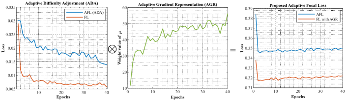
Figure 4: A visualization plot of the gradient correction of FL [37] by the ADA and AGR in this paper. The left figure is the FL after the ADA adjustment. The middle figure is the gradient adjustment value generated by AGR. The right figure is the FL and AFL being adjusted.

Since there is only a quantitative difference between the term of $\nabla_{\mathcal{B}}$ and the gradient term of $\mathbb{\ell}_{\mathrm{bce}}$, we consider $\forall\delta,-\nu_{i}=\delta\times(\nabla_{\mathcal{B}})$, where $\delta\in[0,1]$. Based on the above analysis, we can obtain Eq. (16),

$$\frac{\partial\mathbb{\ell}_{\mathrm{afl}}}{\partial P_{t}} =\sum_{i=1}^{\mathcal{N}}(1-P^{i}_{t})^{\gamma_{\mathrm{d}}}\left[\nu_{i}+\delta\nabla_{\mathcal{B}}\right]$$ (16)

$$=\sum_{i=1}^{\mathcal{N}}(1-P^{i}_{t})^{\gamma_{\mathrm{d}}}\left[(1+\delta\gamma_{\mathrm{d}})\nu_{i}\right],$$

The model classification reaches optimality under the condition that $\sum_{i=1}^{\mathcal{N}}(1-P^{i}_{t})^{\gamma_{\mathrm{d}}}\nu_{i}$ satisfies each $(1-P^{i}_{t})^{\gamma_{\mathrm{d}}}\in\sum_{i=1}^{\mathcal{N}}(1-P^{i}_{t})^{\gamma_{\mathrm{d}}}=0$, and each $\nu_{i}\in\sum_{i=1}^{\mathcal{N}}\nu_{i}=1$. Then, based on Chebyshev’s inequality [60], we can obtain

$$\sum_{i=1}^{\mathcal{N}}(1-P^{i}_{t})^{\gamma_{\mathrm{d}}}\nu_{i}=\tfrac{1}{\mathcal{N}}\sum_{i=1}^{\mathcal{N}}(1-P^{i}_{t})^{\gamma_{\mathrm{d}}}\sum_{i=1}^{\mathcal{N}}\nu_{i},$$ (17)

From this, collating Eq.(13), Eq. (16) with Eq. (17), we can get that Eq. (18)

$$\frac{\partial\mathbb{\ell}_{\mathrm{bce}}}{\partial P_{t}}=\frac{\partial\mathbb{\ell}_{\mathrm{afl}}/\partial P_{t}}{\frac{1}{\mathcal{N}}\sum_{i=1}^{\mathcal{N}}(1-P^{i}_{t})^{\gamma_{\mathrm{d}}}(1+\delta\gamma_{\mathrm{d}})},$$ (18)

Observing Eq. (16) and (18), the gradient of $\mathbb{\ell}_{\mathrm{afl}}$ can be represented as an approximate total gradient of $\mathbb{\ell}_{\mathrm{bce}}$ by introducing an adaptive gradient representation factor $\mu$. For the convenience of the later paper, we let

$$\mu=\frac{\mathcal{N}}{\sum_{i=1}^{\mathcal{N}}{(1-P^{i}_{t})^{\gamma_{\mathrm{d}}}(1+\delta\gamma_{\mathrm{d}}})}.$$ (19)

Based on the above analysis, the designed $\mu$ allows the gradient of the $\mathbb{\ell}_{\mathrm{afl}}$ to be balanced between “Difficulty-equal” and “Difficulty-oriented”, which can increase the weight of low-confidence easy pixels in the training process, thus making the $\mathbb{\ell}_{\mathrm{afl}}$ notice the low-confidence easy pixels rather than focus more on extremely hard pixels.

III-C3 Adaptive Focal Loss

In summary, the proposed $\mathbb{\ell}_{\mathrm{afl}}$ can be expressed as,

$$\mathbb{\ell}_{\mathrm{afl}} =\sum_{i=1}^{\mathcal{N}}\left[-\mu(1-P^{i}_{t})^{\gamma_{\mathrm{d}}}\mathrm{log}(P^{i}_{t})+\alpha(1-P^{i}_{t})^{\gamma_{\mathrm{d}}+1}\right].$$ (20)

On the one hand, AFL allows pixels with smaller $P_{t}$ to obtain higher gradient values for the same $\gamma$ compared with focal loss [37]. When faced with samples with significant differences in pixel difficulty distributions, the $\gamma_{\mathrm{d}}$ of ADA will be increased to overcome inadequate learning. Conversely, when facing samples with minor differences, $\gamma_{\mathrm{d}}$ can adopt a small value to overcome the over-learning of extremely hard pixels. On the other hand, based on the ADA, the $\mu$ of AGR allows the $\mathbb{\ell}_{\mathrm{afl}}$ to be balanced between “Difficulty-equal” and “Difficulty-oriented”, which can increase the weight of low-confidence easy pixels, thus making the $\mathbb{\ell}_{\mathrm{afl}}$ notice the low-confidence easy pixels rather than focus more on extremely hard pixels, yields solving the gradient swamping problem of BCE-based loss.

Such a conclusion can be corroborated in the visualization of Fig. 4; the proposed ADA not only can make the model focus on low-confidence easy pixels but also can produce a larger margin compared to FL [37] (left sub-figure in Fig. 4), which indicates that AFL can adjust the training strategy based on different sample distributions and learning situation. In addition, the ADA can not only make the model focus on low-confidence easy pixels but is also better at maintaining the stability of the model when using AGR directly on FL (right sub-figure in Fig. 4). This is reflected by the fact that the loss value of FL drifts more when AGR is used, while AFL does not.

Moreover, based on the previous theory, it can be easily obtained that when the values of $\mu$ and $\gamma_{\mathrm{d}}$ are 0, the proposed AFL is PL [43]; when $\mu$, $\gamma_{\mathrm{a}}$ and $\alpha$ are 0, the proposed AFL is FL [37]; when $\mu$, $\gamma_{\mathrm{d}}$ and $\alpha$ are 0, the AFL is BCE [42]. This flexible quality allows AFL to achieve higher accuracy when compared to other approaches.

III-D Model Optimization

Let us denote by $\hat{p}_{i}$ the set of click predicted instance permuted according to the optimal permutation $\hat{\mathbb{\sigma}}\in S_{N_{q}}$. Then, we can define our loss function as follows:

Click Loss. We choose the cross-entropy loss as the click loss measure function in this work, and the click loss $\mathbb{L}_{\mathrm{cli}}(\hat{c_{i}},c_{i})$ is intended to compute classification confidence for each pixel, which in turn ensures that each pixel can be computed efficiently.

Mask Loss. We use the proposed AFL (instead of the FL used in [41]) mentioned in Sec.III-B and Dice Loss [50] as the mask loss in this work. Here,

$$\mathbb{L}_{\mathrm{mask}}(\hat{p_{i}},y^{i}_{t})=\lambda_{\mathrm{afl}}\mathbb{\ell}_{\mathrm{afl}}(\hat{p_{i}},y^{i}_{t})+\lambda_{\mathrm{dice}}\mathbb{\ell}_{\mathrm{dice}}(\hat{p_{i}},y^{i}_{t}),$$ (21)

and $\lambda_{\mathrm{afl}}=5.0$, $\lambda_{\mathrm{dice}}=5.0$.

Total Loss. Ultimately, the total loss in this work is the combination of the mask loss and the classification loss,

$$\mathbb{L}_{\mathrm{total}}(\hat{p_{i}},y^{i}_{t})=\sum_{i=1}^{N_{q}}\lambda_{\mathrm{mask}}\mathbb{L}_{\mathrm{mask}}(\hat{p_{i}},y^{i}_{t})+\lambda_{\mathrm{cli}}\mathbb{L}_{\mathrm{cli}}(\hat{p_{i}},y^{i}_{t}).$$ (22)

where $\lambda_{\mathrm{mask}}=1.0$, $\lambda_{\mathrm{cli}}=2.0$. For predictions that match the $\hat{y^{i}_{p}}$ and $0.1$ for “unclick”, i.e., predictions that do not match any ground truth. In particular, we add auxiliary losses to each intermediate transformer decoder layer and learn-able query before decoding with the transformer so that each transformer block can be effectively constrained and thus guarantee the performance of the model.

IV Experiments

In this section, we begin by presenting the datasets utilized in our experiments (Sec. IV-A). Next, Sections IV-B and IV-C outline the implementation specifics and evaluation metrics, followed by an overview of the state-of-the-art models we use for comparison (IV-D). Then, in Sec. IV-E we report detailed quantitative results of our model. This includes a comparative analysis of our proposed AdaptiveClick model with existing state-of-the-art IIS models across nine datasets in Sec. IV-E1 and evaluating our proposed AFL loss against leading loss functions used for IIS, validating its effectiveness and robustness. Finally, Sec. IV-F provides a comprehensive ablation study and a hyperparameter analysis.

IV-A Datasets

We evaluate the proposed AdaptiveClick using the following well-recognized datasets widely used in IIS tasks:

(1) SBD [18]: Comprising $8,498$ images for training and $2,857$ images for testing, this dataset is characterized by its scene diversity and is frequently utilized for the IIS tasks;

(2) COCO [61] + LVIS [62]: This dataset contains $118$K training images ($1.2$M instances), and is a popular choice due to its varying class distributions [8, 28, 61, 53].

(3) GrabCut [63]: The GrabCut dataset contains $50$ images, which have relatively simple appearances and has also been commonly used for evaluating the performance of different IIS methods [8, 28, 61, 53];

(4) Berkeley [64]: This dataset includes $100$ images, sharing some small object images with GrabCut [63]. It poses challenges for IIS models due to these similarities;

(5) DAVIS [65]: Initially designed for video image segmentation, we follow previous work by dividing the $50$ videos into $345$ frames for testing. The dataset features images with high-quality masks.

(6) Pascal VOC [66]: Composed of $1449$ images ($3427$ instances) in the validation dataset, we assess segmentation performance on this validation set, as in [19, 17, 28];

(7) ssTEM [67]: The ssTEM dataset contains two image stacks, each with $20$ medical images. We use the same stack as in [28, 9] to evaluate model effectiveness;

(8) BraTS [68]: The BraTS dataset includes $369$ magnetic resonance images (MRI) volumes. We test our model on the same $369$ slices as in [28, 9];

(9) OAIZIB [69]: OAIZIB dataset consists of $507$ MRI volumes. We test our model on the same $150$ slices ($300$ instances) as in [24, 28];

IV-B Implementation Details

We outline the implementation details of this work.

Data Embedding. The $C$ and $I$ are obtained via patch embedding to encode features $C_{t}$ and $I_{t}$, then they are fused via an addition operation like [8, 28, 23].

Feature Encoding. We use the ViT-Base (ViT-B) and ViT-Huge (ViT-H) as our backbone, which is proposed by [70] and pre-trained as MAEs [71] on ImageNet-1K [72].

Feature Decoding. The designed PMMD is used to encode the fusion feature and then sent to the CAMD, where CAMD consists of three proposed transformer blocks, i.e., $L=3$ ($9$ layers in total), and $Q$ is set to $10.0$.

Post-processing. We multiply the click confidence and the mask confidence (i.e., the average of the foreground pixel-by-pixel binary mask probabilities) to obtain the final confidence matrix and generate the $P_{n}$ as done in [41, 57].

Setup of AdaptiveClick. We train for $60$ epochs on the SBD [18] and the COCO+LVIS dataset [8]; the initial learning rate is set to $5\times 10^{-5}$, and then reduced by $10$ times in the $40$-th epoch. The image is cropped to size $448\times 448$ pix. We choose the CE loss as our Click loss, where $\lambda_{\mathrm{cli}}$ is $2$. The mask loss is a combination of AFL and Dice loss, where $\lambda_{\mathrm{afl}}$ is $5$ and $\lambda_{\mathrm{dice}}$ is $5$. ADAM was used to optimize the training of this model with the parameters $\beta_{1}=0.9$ and $\beta_{2}=0.999$. The batch size is $48$ for training ViT-B and $24$ for training ViT-H, respectively. All experiments are trained and tested on NVIDIA Titan RTX 6000 GPUs.

Setup of Incorporating AFL into State-of-the-Art IIS Methods. We maintained consistency in parameter settings with those of the comparison methods while setting the hyperparameters of the proposed AFL as follows: $\gamma_{\mathrm{d}}=2$ and $\delta=0.4$ during the training process.

TABLE I: Comparison in Noc85 and Noc90 between AdaptiveClick and state-of-the-art methods trained on Augmented VOC [66] and SBD [18] datasets and tested on GrabCut [63], Berkeley [64], SBD [18], DAVIS [65], and Pascal VOC [66] datasets. Top results within a group are indicated in red and the overall top results in bold.

Method	Backbone	Train Data	GrabCut		Berkeley		SBD		DAVIS		Pascal VOC
			Noc85	Noc90	Noc85	Noc90	Noc85	Noc90	Noc85	Noc90	Noc85	Noc90
DIOS [27] CVPR2016	FCN	Augmented VOC	-	$6.04$	-	$8.65$	-	-	-	$12.58$	$6.88$	-
FCANet [17] CVPR2020	ResNet101	Augmented VOC	-	$2.08$	-	$3.92$	-	-	-	$7.57$	$2.69$	-
Latent Diversity [20] CVPR2018	VGG-19	SBD	$3.20$	$4.79$	-	-	$7.41$	$10.78$	$5.05$	$9.57$	-	-
BRS [25] CVPR2019	DenseNet	SBD	$2.60$	$3.60$	-	$5.08$	$6.59$	$9.78$	$5.58$	$8.24$	-	-
IA-SA [39] ECCV2020	ResNet101	SBD	-	$3.07$	-	$4.94$	-	-	$5.16$	-	-	-
f-BRS-B [26] CVPR2020	ResNet50	SBD	$2.50$	$2.98$	-	$4.34$	$5.06$	$8.08$	$5.39$	$7.81$	-	-
CDNet [19] CVPR2021	ResNet34	SBD	$1.86$	$2.18$	$1.95$	$3.27$	$5.18$	$7.89$	$5.00$	$6.38$	-	-
RITM [8] ICIP2022	HRNet18	SBD	$1.76$	$2.04$	1.87	$3.22$	$3.39$	$5.43$	$4.94$	$6.71$	$2.51$	$3.03$
PseudoClick [9] ECCV2022	HRNet18	SBD	$1.68$	$2.04$	$1.85$	$3.23$	$3.38$	$5.40$	$4.81$	$6.57$	${\color[rgb]{1,0,0}2.34}$	${\color[rgb]{1,0,0}2.74}$
FocalClick [23] CVPR2022	SegF-B0	SBD	$1.66$	$1.90$	-	$3.14$	$4.34$	$6.51$	$5.02$	$7.06$	-	-
Fcouscut [10] CVPR2022	ResNet101	SBD	$1.46$	$1.64$	$1.81$	$3.01$	$3.40$	$5.31$	$4.85$	$6.22$	-	-
GPCIS [53] CVPR2023	SegF-B0	SBD	$1.60$	$1.76$	$1.84$	$2.70$	$4.16$	$6.28$	$4.45$	$6.04$	-	-
FCFI [29] CVPR2023	ResNet101	SBD	$1.64$	$1.80$	-	$2.84$	${\color[rgb]{1,0,0}3.26}$	$5.35$	$4.75$	$6.48$	-	-
SimpleClick [28] Arxiv2023	ViT-B	SBD	${\color[rgb]{1,0,0}1.40}$	${\color[rgb]{1,0,0}1.54}$	${\color[rgb]{1,0,0}1.44}$	${\color[rgb]{1,0,0}2.46}$	$3.28$	${\color[rgb]{1,0,0}5.24}$	${\color[rgb]{1,0,0}4.10}$	${\color[rgb]{1,0,0}5.48}$	$2.38$	$2.81$
AdaptiveClick (Ours)	ViT-B	SBD	1.38	1.46	1.38	2.18	3.22	5.22	4.00	5.14	2.25	2.66

TABLE II: Comparison in Noc85 and Noc90 between AdaptiveClick and state-of-the-art methods trained on the COCO-LVIS dataset [8] and tested on GrabCut [63], Berkeley [64], SBD [18], DAVIS [65], and Pascal VOC [66] datasets.

Method	Backbone	Train Data	GrabCut		Berkeley		SBD		DAVIS		Pascal VOC
			Noc85	Noc90	Noc85	Noc90	Noc85	Noc90	Noc85	Noc90	Noc85	Noc90
f-BRS-B [26] CVPR2020	HRNet32	COCO-LVIS	$1.54$	$1.69$	-	$2.44$	$4.37$	$7.26$	$5.17$	$6.50$	-	-
CDNet [19] ICCV2021	ResNet-34	COCO-LVIS	$1.40$	$1.52$	$1.47$	$2.06$	$4.30$	$7.04$	$4.27$	$5.56$	$2.74$	$3.30$
RITM [8] ICIP2022	HRNet32	COCO-LVIS	$1.46$	$1.56$	$1.43$	$2.10$	$3.59$	$5.71$	$4.11$	$5.34$	$2.19$	$2.57$
Pseudo click [9] ECCV2022	HRNet32	COCO-LVIS	$1.36$	$1.50$	$1.40$	$2.08$	$3.38$	$5.54$	$3.79$	$5.11$	$1.94$	$2.25$
FocalClick [23] CVPR2022	SegF-B0	COCO-LVIS	$1.40$	$1.66$	$1.59$	$2.27$	$4.56$	$6.86$	$4.04$	$5.49$	$2.97$	$3.52$
FocalClick [23] CVPR2022	SegF-B3	COCO-LVIS	$1.44$	$1.50$	$1.55$	$1.92$	$3.53$	$5.59$	$3.61$	$4.90$	$2.46$	$2.88$
FCFI [29] CVPR2023	HRNet18	COCO-LVIS	$1.38$	$1.46$	-	$1.96$	$3.63$	$5.83$	$3.97$	$5.16$	-	-
DynaMITe [32] Arxiv2023	SegF-B3	COCO-LVIS	$1.48$	$1.58$	$1.34$	$1.97$	$3.81$	$6.38$	$3.81$	$5.00$	-	-
† SAM [30] Arxiv2023	ViT-B	COCO-LVIS	-	-	-	-	$6.50$	$9.76$	-	-	$3.30$	$4.20$
† SEEM [33] Arxiv2023	DaViT-B	COCO-LVIS	-	-	-	-	$6.67$	$9.99$	-	-	$3.41$	$4.33$
InterFormer [31] Arxiv2023	ViT-B	COCO-LVIS	$1.38$	$1.50$	$1.99$	$3.14$	$3.78$	$6.34$	$4.10$	$6.19$	-	-
InterFormer [31] Arxiv2023	ViT-L	COCO-LVIS	1.26	1.36	$1.61$	$2.53$	$3.25$	$5.51$	$4.54$	$5.21$	-	-
SimpleClick [28] Arxiv2023	ViT-H	COCO-LVIS	$1.38$	$1.50$	${\color[rgb]{1,0,0}1.36}$	${\color[rgb]{1,0,0}1.75}$	${\color[rgb]{1,0,0}2.85}$	${\color[rgb]{1,0,0}4.70}$	${\color[rgb]{1,0,0}3.41}$	${\color[rgb]{1,0,0}4.78}$	${\color[rgb]{1,0,0}1.76}$	${\color[rgb]{1,0,0}1.98}$
AdaptiveClick (Ours)	ViT-H	COCO-LVIS	${\color[rgb]{1,0,0}1.32}$	${\color[rgb]{1,0,0}1.38}$	1.32	1.64	2.84	4.68	3.19	4.60	1.74	1.96
† denotes this method as a universal image segmentation model, and in this paper, we cite their accuracy in the IIS task.

TABLE III: Comparison in Noc85 and Noc90 between AdaptiveClick and state-of-the-art methods trained on the SBD dataset [18] and tested on ssTEM [63], BraTS [64], and OAIZIB [64] datasets.

Method	Backbone	Train Data	ssTEM		BraTS		OAIZIB
			Noc85	Noc90	Noc85	Noc90	Noc85	Noc90
CDNet [19] ICCV2021	ResNet-34	SBD	$11.10$	$14.65$	$17.07$	$18.86$	$19.56$	$19.95$
RITM [8] ICIP2022	HRNet18	SBD	${\color[rgb]{1,0,0}3.71}$	$5.68$	8.47	12.59	${\color[rgb]{1,0,0}17.70}$	${\color[rgb]{1,0,0}19.95}$
SimpleClick [28] Arxiv2023	ViT-B	SBD	$3.78$	${\color[rgb]{1,0,0}5.21}$	${\color[rgb]{1,0,0}9.93}$	${\color[rgb]{1,0,0}13.90}$	$18.44$	$19.90$
AdaptiveClick (Ours)	ViT-B	SBD	3.17	4.56	$10.79$	$14.39$	17.43	19.62

TABLE IV: Comparison in Noc85 and Noc90 between AdaptiveClick and state-of-the-art methods trained on the COCO-LVIS [8] and tested on ssTEM [63], BraTS [64], and OAIZIB [64] datasets.

Method	Backbone	Train Data	ssTEM		BraTS		OAIZIB
			Noc85	Noc90	Noc85	Noc90	Noc85	Noc90
CDNet [19] ICCV2021	ResNet-34	COCO-LVIS	$4.15$	$8.45$	$10.51$	$14.80$	$17.42$	$19.81$
RITM [8] ICIP2022	HRNet32	COCO-LVIS	2.74	4.06	$7.56$	$11.24$	$15.89$	$19.27$
FocalClick [23] CVPR2022	SegF-B3	COCO-LVIS	$3.95$	$5.05$	$7.17$	$11.19$	${\color[rgb]{1,0,0}12.93}$	$19.23$
SimpleClick [28] Arxiv2023	ViT-H	COCO-LVIS	$4.27$	$5.45$	${\color[rgb]{1,0,0}6.73}$	${\color[rgb]{1,0,0}10.27}$	$14.93$	${\color[rgb]{1,0,0}18.95}$
AdaptiveClick (Ours)	ViT-H	COCO-LVIS	${\color[rgb]{1,0,0}3.95}$	${\color[rgb]{1,0,0}4.97}$	6.51	9.77	12.65	16.69

IV-C Evaluation Metrics

Following previous works [8, 73, 17], we select NoC IoU $0.85$ (Noc85) and $0.9$ (Noc90) as evaluation metrics, with the maximum NoC set to 20 (samples with $NoC>20$ are considered failures. The lower the value of the Noc85 and Noc90 metrics, the better. We also use the average IoU given $k$ clicks (mIoU@$k$) as an evaluation metric to measure the segmentation quality given a fixed number of clicks.

IV-D Compared Methods

We validate our approach against state-of-the-art IIS methods and loss functions, specifically:

IIS Methods. Our comparison include state-of-the-art IIS methods including DIOS [27], Latent diversity [20], BRS [25], f-BRS-B [26], IA-SA [39], FCA-Net [17], PseudoClick [9], CDNet [19], RITM [8], FocalClick [23], FocusCut [10], GPCIS [53], SimpleClick [28], FCFI [29], InterFormer [31], DynaMITe [32], SAM [30], and SEEM [33], all of which achieve competitive results.

Loss Functions. We compare the proposed AFL loss with state-of-the-art loss functions, including BCE [42], Soft IoU [49], FL [37], NFL [52], WBCE [44], Balanced CE [45], and Poly [43] losses, which are widely used in IIS and semantic segmentation tasks [51].

IV-E Model Analysis

In this section, we present a comprehensive analysis of the experimental results. We compare the segmentation quality of the proposed AdaptiveClick with the state-of-the-art methods using two training datasets and eight test datasets.

IV-E1 Comparison with State-of-the-Art Methods

TABLE I and TABLE II empirically analyze the performance of AdaptiveClick and state-of-the-art methods using SBD and COCO+LIVS as training datasets. Likewise, TABLE III and TABLE IV display the performance of AdaptiveClick and relevant published methods in medical images, respectively.

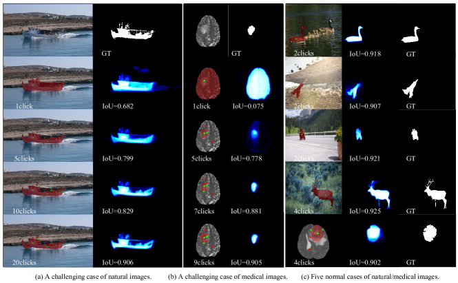
Figure 5: Segmentation results on natural and medical datasets. The backbone model is ViT-B trained on the SBD dataset [18]. The segmentation probability maps are shown in blue; the segmentation maps are overlaid in red on the original images. The clicks are shown as green (positive click) or red (negative click) dots on the image. GT denotes ground truth.

Evaluation on the Natural Images. As shown in TABLE I and TABLE II, we compare AdaptiveClick with state-of-the-art methods for existing IIS tasks. First, we present the experimental comparison of AdaptiveClick using a lightweight model. Employing ViT-B and ViT-H as the backbone and the proposed AFL as the loss function, AdaptiveClick achieves an average accuracy improvement of $0.074$, $0.174$, and $0.07$, $0.09$ on SBD and COCO+LIVS, respectively, compared to existing state-of-the-art methods on NoC85 and NoC90. This demonstrates that the proposed AdaptiveClick exhibits greater robustness and superior accuracy performance in handling interaction ambiguity and gradient swamping.

TABLE V: Evaluation of the AdaptiveClick with ViT-B trained on SBD [18] with different loss functions. We report Noc85 and Noc90 on GrabCut [63], Berkeley [64], SBD [18], DAVIS [65], and Pascal VOC [66] datasets.

Method	GrabCut		Berkeley		SBD		DAVIS		Pascal VOC
	Noc85	Noc90	Noc85	Noc90	Noc85	Noc90	Noc85	Noc90	Noc85	Noc90
BCE [42] ISIMP04	$1.64$	$1.78$	$1.69$	$2.99$	$4.06$	$6.39$	$4.55$	$6.08$	$2.85$	$3.37$
WBCE [44] Bioinf.07	$1.66$	$2.58$	$2.25$	$5.20$	$5.18$	$8.00$	$5.43$	$9.28$	$3.39$	$4.12$
Balanced CE [45] ICCV15	$1.62$	$1.84$	$1.88$	$3.59$	$4.55$	$7.00$	$5.57$	$7.35$	$3.44$	$4.18$
Soft IoU [49] ISVC16	$1.62$	$1.99$	$1.78$	$2.29$	$4.55$	$6.48$	$4.69$	$6.32$	$3.13$	$3.71$
FL [37] ICCV17	$1.62$	$1.84$	$1.69$	$2.82$	$4.11$	$6.51$	$4.94$	$6.50$	$2.81$	$3.35$
NFL [52] ICCV19	${\color[rgb]{1,0,0}1.40}$	${\color[rgb]{1,0,0}1.50}$	1.32	${\color[rgb]{1,0,0}2.24}$	${\color[rgb]{1,0,0}3.25}$	${\color[rgb]{1,0,0}5.28}$	${\color[rgb]{1,0,0}4.03}$	${\color[rgb]{1,0,0}5.24}$	${\color[rgb]{1,0,0}2.30}$	${\color[rgb]{1,0,0}2.75}$
Poly Loss [45] ICLR22	$1.46$	$1.70$	$1.68$	$2.87$	$4.09$	$6.42$	$4.70$	$6.43$	$2.85$	$3.39$
AFL (Ours)	1.38	1.46	${\color[rgb]{1,0,0}1.38}$	2.18	3.22	5.22	4.00	5.14	2.25	2.66

Evaluation on Medical Image Segmentation. As demonstrated in TABLE III and TABLE IV, we present the comparative results of AdaptiveClick and state-of-the-art IIS methods for medical image segmentation tasks. It is worth noting that existing IIS methods generally exhibit suboptimal performance when applied to medical image segmentation. This can be attributed to two factors. First, the majority of IIS methods have not been trained on specialized medical datasets, even though some studies have introduced such datasets for training purposes [74]. Second, these IIS methods tend to exhibit limited generalization capabilities. In contrast, AdaptiveClick maintains consistently high segmentation quality across various tasks, including medical image segmentation, showcasing the method’s versatility. Fig. 5 visually compares different segmentation methods in the context of natural images, medical images with challenging scenarios, and normal examples.

IV-E2 Effectiveness of Adaptive Focal Loss

TABLE VI: Evaluation of the AdaptiveClick of ViT-B trained on COCO+LVIS [8] with different loss functions. We report Noc85 and Noc90 on GrabCut [63], Berkeley [64], SBD [18], DAVIS [65], and Pascal VOC [66] datasets.

Method	GrabCut		Berkeley		SBD		DAVIS		Pascal VOC
	Noc85	Noc90	Noc85	Noc90	Noc85	Noc90	Noc85	Noc90	Noc85	Noc90
BCE [42] ISIMP04	$1.54$	$1.72$	$1.79$	$2.89$	$4.30$	$6.74$	$4.29$	$5.76$	$2.71$	$3.19$
WBCE [44] Bioinf.07	$1.60$	$1.88$	$2.15$	$4.29$	$5.60$	$8.61$	$5.26$	$8.79$	$3.32$	$4.03$
Balanced CE [45] ICCV15	$1.74$	$2.10$	$2.13$	$4.32$	$5.53$	$8.58$	$4.90$	$8.02$	$3.24$	$3.93$
Soft IoU [49] ISVC16	$1.62$	$1.70$	$1.64$	$2.63$	$4.19$	$6.66$	$4.19$	$5.60$	$2.69$	$3.18$
FL [37] ICCV17	$1.54$	$1.60$	$1.58$	$2.62$	$4.19$	$6.60$	$4.12$	$5.60$	$2.64$	$3.12$
NFL [52] ICCV19	1.34	${\color[rgb]{1,0,0}1.54}$	${\color[rgb]{1,0,0}1.55}$	${\color[rgb]{1,0,0}1.92}$	${\color[rgb]{1,0,0}3.34}$	${\color[rgb]{1,0,0}5.48}$	${\color[rgb]{1,0,0}3.66}$	${\color[rgb]{1,0,0}4.93}$	${\color[rgb]{1,0,0}2.06}$	${\color[rgb]{1,0,0}2.39}$
Poly Loss [45] ICLR22	$1.50$	$1.66$	$1.66$	$2.85$	$4.26$	$6.74$	$4.32$	$5.68$	$2.71$	$3.19$
AFL (Ours)	1.34	1.48	1.40	1.83	3.29	5.40	3.39	4.82	2.03	2.31

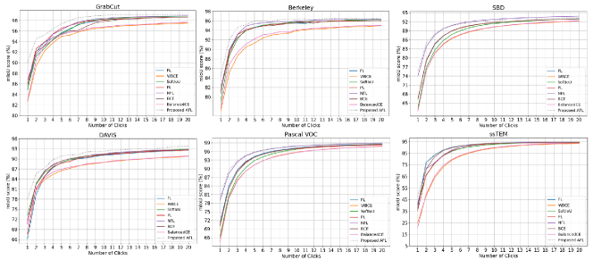
Figure 6: The convergence analysis between the proposed AFL and other state-of-the-art loss functions. In this experiment, AdaptiveClick is used as the benchmark framework and SBD [18] as the training dataset. The test results are reported for GrabCut [63], Berkeley [64], SBD [18], DAVIS [65], Pascal VOC [66], and ssTEM [63] datasets, respectively. The metric is mean IoU given k clicks. Overall, our models require fewer clicks for a given accuracy level. The compared loss functions from top to bottom are FL [37], WBCE [44], Soft IoU [49], Poly [43], NFL [52], BCE [42], Balanced CE [45], and proposed AFL loss, respectively. Our AdaptiveClick in general requires fewer clicks for a given accuracy level.

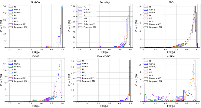
Figure 7: The histogram analysis between the proposed AFL and other state-of-the-art loss functions. In this experiment, AdaptiveClick is used as the benchmark framework and COCO + LVIS [8] as the training dataset. The test results are reported for GrabCut [63], Berkeley [64], SBD [18], DAVIS [65], Pascal VOC [66], and ssTEM [63] datasets, respectively. The compared loss functions from top to bottom are FL [37], WBCE [44], Soft IoU [49], Poly [43], NFL [52], BCE [42], Balanced CE [45], and the proposed AFL loss, respectively. Given $k=4$ clicks. Our AdaptiveClick obtains the best segmentation results (more instances with higher IoU) than the other seven comparison loss functions.

Comparison with State-of-the-Art Loss Functions. The performance of different loss functions on the SBD [18] and COCO+LIVS [8] datasets are illustrated in TABLEs V, VI, respectively. TABLE V demonstrates that the proposed AFL achieves an average improvement of $0.014{\sim}0.07$ and $1.136{\sim}2.504$ on NoC85 and NoC90, respectively (SBD training dataset) when compared to BCE, WBCE, Balanced CE, FL, NFL, and PL. This indicates that, as analyzed in Equations (13) and (14), both BCE and FL-based losses exhibit a certain degree of gradient swamping, and the proposed AFL can effectively mitigate this issue. A comparison of the experimental results for AFL with WBCE, BalancedCE, and SoftIoU reveals that although these losses account for the pixel imbalance problem in segmentation, they do not excel in the IIS task, as the more profound gradient swamping issue has not been adequately addressed. Fig. 6 displays the mean IoU performance for each loss function, confirming that the AFL consistently improves performance across all six datasets.

TABLE VII: Results in Noc85 and Noc90 for state-of-the-art methods with and without with proposed adaptive focal loss. In these experiments, we trained on the SBD [18] and tested on GrabCut [63], Berkeley [64], SBD [18], DAVIS [65], and Pascal VOC [66] datasets. It should be noted that AdaptiveClick + NFL indicates the results obtained by using AdaptiveClick, but using NFL [52] as the training loss. AdaptiveClick, on the other hand, indicates the results obtained by using both the framework of this paper and the AFL loss functions. Top results within a group are indicated in red.

Method

Backbone

Train Data

GrabCut

Berkeley

SBD

DAVIS

Pascal VOC

Noc85

Noc90

Noc85

Noc90

Noc85

Noc90

Noc85

Noc90

Noc85

Noc90

CDNet [19] CVPR2021

ResNet34

SBD

$1.86$

$2.18$

$1.95$

$3.27$

$5.18$

$7.89$

$5.00$

$6.38$

-

-

CDNet (Ours)

ResNet34

SBD

${\color[rgb]{1,0,0}1.82}$

${\color[rgb]{1,0,0}2.14}$

${\color[rgb]{1,0,0}1.86}$

${\color[rgb]{1,0,0}2.88}$

${\color[rgb]{1,0,0}4.53}$

${\color[rgb]{1,0,0}7.15}$

${\color[rgb]{1,0,0}4.78}$

${\color[rgb]{1,0,0}6.27}$

-

-

RITM [8] ICIP2022

HRNet18

SBD

$1.76$

$2.04$

1.87

$3.22$

${\color[rgb]{1,0,0}3.39}$

$5.43$

$4.94$

$6.71$

$2.51$

$3.03$

RITM (Ours)

HRNet18

SBD

${\color[rgb]{1,0,0}1.60}$

${\color[rgb]{1,0,0}1.86}$

${\color[rgb]{1,0,0}1.72}$

${\color[rgb]{1,0,0}2.93}$

$3.40$

${\color[rgb]{1,0,0}5.42}$

${\color[rgb]{1,0,0}4.72}$

${\color[rgb]{1,0,0}6.15}$

${\color[rgb]{1,0,0}2.41}$

${\color[rgb]{1,0,0}2.92}$

FocalClick [23] CVPR2022

SegF-B0

SBD

$1.66$

$1.90$

-

$3.14$

${\color[rgb]{1,0,0}4.34}$

$6.51$

$5.02$

$7.06$

-

-

FocalClick (Ours)

SegF-B0

SBD

${\color[rgb]{1,0,0}1.64}$

${\color[rgb]{1,0,0}1.84}$

-

${\color[rgb]{1,0,0}3.12}$

$4.36$

${\color[rgb]{1,0,0}6.44}$

${\color[rgb]{1,0,0}4.79}$

${\color[rgb]{1,0,0}6.50}$

-

-

Fcouscut [10] CVPR2022

ResNet50

SBD

$1.60$

$1.78$

$1.85$

$3.44$

$3.62$

$5.66$

$5.00$

$6.38$

-

-

Fcouscut (Ours)

ResNet50

SBD

${\color[rgb]{1,0,0}1.54}$

${\color[rgb]{1,0,0}1.72}$

${\color[rgb]{1,0,0}1.79}$

${\color[rgb]{1,0,0}3.34}$

${\color[rgb]{1,0,0}3.50}$

${\color[rgb]{1,0,0}5.62}$

${\color[rgb]{1,0,0}4.82}$

${\color[rgb]{1,0,0}6.28}$

-

-

SimpleClick [28] Arxiv2023

ViT-B

SBD

$1.40$

$1.54$

${\color[rgb]{1,0,0}1.44}$

$2.46$

$3.28$

$5.24$

${\color[rgb]{1,0,0}4.10}$

${\color[rgb]{1,0,0}5.48}$

$2.38$

$2.81$

SimpleClick (Ours)

ViT-B

SBD

${\color[rgb]{1,0,0}1.36}$

${\color[rgb]{1,0,0}1.52}$

${\color[rgb]{1,0,0}1.44}$

${\color[rgb]{1,0,0}2.34}$

${\color[rgb]{1,0,0}3.10}$

${\color[rgb]{1,0,0}5.04}$

${\color[rgb]{1,0,0}4.10}$

$5.51$

${\color[rgb]{1,0,0}2.23}$

${\color[rgb]{1,0,0}2.63}$

AdaptiveClick + NFL

ViT-B

SBD

$1.40$

$1.50$

${\color[rgb]{1,0,0}1.32}$

$2.24$

$3.25$

$5.28$

$4.03$

$5.24$

$2.30$

$2.75$

AdaptiveClick (Ours)

ViT-B

SBD

${\color[rgb]{1,0,0}1.38}$

${\color[rgb]{1,0,0}1.46}$

$1.38$

${\color[rgb]{1,0,0}2.18}$

${\color[rgb]{1,0,0}3.22}$

${\color[rgb]{1,0,0}5.22}$

${\color[rgb]{1,0,0}4.00}$

${\color[rgb]{1,0,0}5.14}$

${\color[rgb]{1,0,0}2.25}$

${\color[rgb]{1,0,0}2.66}$

TABLE VIII: Results in Noc85 and Noc90 results for state-of-the-art methods with and without the proposed adaptive focal loss. In these experiments, we trained on the COCO-LVIS dataset [8] and tested on the GrabCut [63], Berkeley [64], SBD [18], DAVIS [65], and Pascal VOC [66] datasets.

Method

Backbone

Train Data

GrabCut

Berkeley

SBD

DAVIS

Pascal VOC

Noc85

Noc90

Noc85

Noc90

Noc85

Noc90

Noc85

Noc90

Noc85

Noc90

RITM [8] ICIP2022

HRNet32

COCO-LVIS

$1.46$

$1.56$

$1.43$

$2.10$

$3.59$

$5.71$

$4.11$

$5.34$

$2.19$

$2.57$

RITM (Ours)

HRNet32

COCO-LVIS

${\color[rgb]{1,0,0}1.42}$

${\color[rgb]{1,0,0}1.51}$

${\color[rgb]{1,0,0}1.40}$

${\color[rgb]{1,0,0}1.98}$

${\color[rgb]{1,0,0}3.48}$

${\color[rgb]{1,0,0}5.64}$

${\color[rgb]{1,0,0}3.69}$

${\color[rgb]{1,0,0}5.26}$

${\color[rgb]{1,0,0}2.10}$

${\color[rgb]{1,0,0}2.54}$

FocalClick [23] CVPR2022

SegF-B3

COCO-LVIS

$1.44$

$1.50$

$1.55$

$1.92$

$3.53$

$5.59$

$3.61$

$4.90$

$2.46$

$2.88$

FocalClick (Ours)

SegF-B3

COCO-LVIS

${\color[rgb]{1,0,0}1.40}$

${\color[rgb]{1,0,0}1.44}$

${\color[rgb]{1,0,0}1.52}$

${\color[rgb]{1,0,0}1.87}$

${\color[rgb]{1,0,0}3.51}$

${\color[rgb]{1,0,0}5.49}$

${\color[rgb]{1,0,0}3.57}$

${\color[rgb]{1,0,0}4.85}$

${\color[rgb]{1,0,0}2.44}$

${\color[rgb]{1,0,0}2.86}$

SimpleClick [28] Arxiv2023

ViT-H

COCO-LVIS

${\color[rgb]{1,0,0}1.38}$

${\color[rgb]{1,0,0}1.50}$

$1.36$

$1.75$

$2.85$

$4.70$

$3.41$

$4.78$

$1.76$

$1.98$

SimpleClick (Ours)

ViT-H

COCO-LVIS

$1.40$

${\color[rgb]{1,0,0}1.50}$

${\color[rgb]{1,0,0}1.33}$

${\color[rgb]{1,0,0}1.71}$

${\color[rgb]{1,0,0}2.80}$

${\color[rgb]{1,0,0}4.65}$

${\color[rgb]{1,0,0}3.23}$

${\color[rgb]{1,0,0}4.75}$

${\color[rgb]{1,0,0}1.72}$

${\color[rgb]{1,0,0}1.93}$

InterFormer [31] Arxiv2023

ViT-L

COCO-LVIS

$1.28$

$1.36$

$1.61$

$2.53$

$3.25$

$5.51$

$4.54$

$5.21$

-

-

InterFormer (Ours)

ViT-L

COCO-LVIS

${\color[rgb]{1,0,0}1.26}$

${\color[rgb]{1,0,0}1.32}$

${\color[rgb]{1,0,0}1.56}$

${\color[rgb]{1,0,0}2.50}$

${\color[rgb]{1,0,0}3.21}$

${\color[rgb]{1,0,0}5.46}$

${\color[rgb]{1,0,0}4.48}$

${\color[rgb]{1,0,0}5.18}$

-

-

AdaptiveClick + NFL

ViT-B

COCO-LVIS

${\color[rgb]{1,0,0}1.34}$

$1.54$

$1.55$

$1.92$

$3.34$

$5.48$

$3.66$

$4.93$

$2.06$

$2.39$

AdaptiveClick (Ours)

ViT-B

COCO-LVIS

${\color[rgb]{1,0,0}1.34}$

${\color[rgb]{1,0,0}1.48}$

${\color[rgb]{1,0,0}1.40}$

${\color[rgb]{1,0,0}1.83}$

${\color[rgb]{1,0,0}3.29}$

${\color[rgb]{1,0,0}5.40}$

${\color[rgb]{1,0,0}3.39}$

${\color[rgb]{1,0,0}4.82}$

${\color[rgb]{1,0,0}2.03}$

${\color[rgb]{1,0,0}2.31}$

We also report the segmentation quality achieved with AFL with the COCO+LIVS training dataset. The results in TABLE VI showcase that the proposed AFL significantly boosts the IIS model performance when compared to other state-of-the-art loss functions, which is consistent with the outcome observed using the SBD training dataset. Fig. 7 shows the IoU statistics on the test dataset with $4$ clicks. It becomes evident that the proposed AFL always maintains the highest IoU and count values for the same number of hits, which confirms that the proposed AFL has stronger robustness and better accuracy compred with different loss functions.

Overall, the proposed AFL significantly enhances the performance of the IIS model and consistently outperforms existing loss functions designed for IIS tasks.

Embedding AFL into State-of-the-Art IIS Methods. TABLE VII and TABLE VIII report the experimental results of embedding AFL into existing state-of-the-art models on SBD and COCO+LIVS training datasets, respectively. In this experiment, we consider state-of-the-art models with different backbones [10, 8, 23, 28] (e.g., ResNet, HRNet, SegFormer, and ViT, etc.), different loss functions [10, 8, 28] (e.g., BCE, SoftIoU, FL, NFL, etc.), and different types of architectures [19, 8, 28, 31] (e.g., CNNs and Transformer) to verify the robustness and generalization.

TABLE IX: Ablation studies by using or not using CAMD and AFL training on SBD [18] and testing on GrabCut [63], Berkeley [64], SBD [18], DAVIS [65], and Pascal VOC [66] datasets. The default choice is colored in yellow.

CAMD	AFL	GrabCut		Berkeley		SBD		DAVIS		Pascal VOC
		Noc85	Noc90	Noc85	Noc90	Noc85	Noc90	Noc85	Noc90	Noc85	Noc90
		$1.46$	$1.58$	$1.56$	$2.46$	$3.28$	$5.32$	$4.20$	$5.79$	$2.42$	$2.85$
$\surd$		$1.40$	$1.50$	1.32	$2.24$	$3.25$	$5.28$	$4.03$	$5.24$	$2.30$	$2.75$
	$\surd$	$1.42$	$1.60$	$1.58$	$2.35$	$3.29$	$5.26$	$4.15$	$5.55$	$2.33$	$2.73$
$\surd$	$\surd$	1.38	1.46	$1.38$	2.18	3.22	5.22	4.00	5.14	2.25	2.66

TABLE X: Ablation studies by using or not using proposed ADA and AGR of AFL training on SBD [18] and testing on the GrabCut [63], Berkeley [64], SBD [18], DAVIS [65], and Pascal VOC [66] datasets.

ADA	AGR	GrabCut		Berkeley		SBD		DAVIS		Pascal VOC
		Noc85	Noc90	Noc85	Noc90	Noc85	Noc90	Noc85	Noc90	Noc85	Noc90
		$1.62$	$1.84$	$1.69$	$2.82$	$4.11$	$6.51$	$4.94$	$6.50$	$2.81$	$3.35$
$\surd$		$1.50$	$1.60$	$1.64$	$2.57$	$3.83$	$6.03$	$4.36$	$5.78$	$2.63$	$3.12$
	$\surd$	$1.56$	$1.68$	$1.54$	$2.40$	$3.27$	$5.23$	$4.50$	$5.82$	$2.32$	$2.74$
$\surd$	$\surd$	1.38	1.46	1.38	2.18	3.22	5.22	4.00	5.14	2.25	2.66

As shown in TABLE VII, the proposed AFL brings positive effect improvements for almost all compared methods in all experiments on the test dataset. This indicates that AFL is robust enough to be applicable to existing mainstream IIS models. Further, the proposed AFL can bring an average Noc85 and Noc90 performance gain of $0.137$, $0.181$ and $0.119$, $0.103$ for CNN- and transformer-based IIS methods, respectively. Comparing the performance of Focalclick, SimpleClick, and AdaptiveClick, it can be seen that the proposed AFL is able to deliver Noc85 and Noc90 improvements for Focalclick, SimpleClick, and AdaptiveClick by $0.23$, $0.114$, $0.014$, $0.142$, and $0.098$, $0.07$, respectively, on the five mainstream test datasets. Comparing the results of CDNet, RITM, and Focuscut, it is clear that the proposed AFL can not only significantly improve the accuracy of the transformer-based model, but also brings performance gains to the CNNs-based model. This reflects that AFL has more performance gains for transformer-based models and certifies that AFL has the potential to unleash the capacity of vision transformers in IIS tasks. Consistent with the above analysis, the same results are confirmed in TABLE VIII on the metrics with COCO+LIVS as the training dataset. In summary, AFL can be applied to different training and test datasets and can adapt to different backbones, loss functions, and different architectures of IIS models with performance gains and strong generalizability.

IV-F Ablation Studies

In this section, we explore the effectiveness of the proposed components on the performance to verify the effectiveness of the components in AdaptiveClick.

IV-F1 Influence of Components in AdaptiveClick

Influence of Components in AdaptiveClick As in TABLE IX, we first show the performance changes with and without the proposed CAMD component on the AdaptiveClick. The use of the CAMD is effective in improving the performance on the five test datasets. This positive performance justifies our analysis of the existing mask-fixed model in Sec. III-A. At the same time, it confirms that the CAMD can effectively solve the interaction ambiguity problem, and the designed CAAM component can provide for long-range propagation between clicks.

To further explore the effect of AFL on the IIS model, we report the performance of the AdaptiveClick when only AFL is used. As seen from the TABLEs, the model’s performance on GrabCut and the DAVIS dataset is already close to that of the full AdaptiveClick when only AFL is used. This indicates that the proposed AFL has strong robustness. With both CAMD and AFL, the model’s performance greatly improved on all five test datasets, which indicates that the proposed CAMD and AFL can effectively address the problems of “interaction ambiguity” in existing IIS tasks.

Influence of Components in AFL. In TABLE X, the focal loss does not perform satisfactorily without using any of the proposed components. In contrast, the model’s performance improves clearly on all five test datasets after using the proposed ADA component. This indicates that the proposed ADA component can help the model adjust the learning strategy adaptively according to differences in sample difficulty and number distribution. At the same time, the first hypothesis proposed in Sec. III-C1, that giving a fixed $\gamma$ to all training samples of a dataset is a suboptimal option that may prevent achieving satisfactory performance on low-confidence easy pixels, is verified, which proves the rationality and effectiveness of the proposed ADA component.

Also, we explored the case of using only the AGR component. The use of AGR results in more significant performance gains on the Berkeley, SBD, and PasvalVOC test datasets compared to the ADA-only component. This indicates the effectiveness of the proposed AGR component and validates the second hypothesis proposed in Sec. III-C1, that FL has the problem that when one wants to increase the concentration on learning with severe hard-easy imbalance, it tends to sacrifice part of low-confidence easy pixels’ loss contribution in the overall training process. At the same time, this proves the validity of the theoretical analysis in Sec. III-C1. Namely, the gradient direction of the simulated BCE can help AFL classify low-confidence easy pixels.

Finally, when both ADA and AGR components are used, AFL brings a minimum gain of $0.14$, $0.34$ (on the GrabCut dataset) and a maximum gain of $0.94$, $1.23$ (on DAVIS and SBD datasets) over FL on the NoC85 and NoC90 evaluation metrics, respectively. Such significant performance improvements again demonstrate the effectiveness of the AFL.

IV-G Influence of the Hyper-parameter

To investigate the effect of the main hyperparameters of the model on the performance, we organized the following experiments. First, the effects of $\lambda_{\mathrm{cli}}$, $\lambda_{\mathrm{afl}}$, $\lambda_{\mathrm{dice}}$, and $Q$ on the model performance are explored, and the main experimental results are shown in TABLE XI. Then, the effect of the delta ($\delta$) parameter in AFL on the model was explored. TABLE XII reports the accuracy changes in Noc85 and Noc90 on five test datasets for different values of $\delta$.

TABLE XI: The impact of different hyperparameter settings on AdaptiveClick. We trained our AdaptiveClick on the SBD [18] and tested on GrabCut [63], Berkeley [64], SBD [18], DAVIS [65], and Pascal VOC [66] datasets.

$\lambda_{\mathrm{cli}}$	$\lambda_{\mathrm{afl}}$	$\lambda_{\mathrm{dice}}$	$Q$	GrabCut		Berkeley		SBD		DAVIS		Pascal VOC
				Noc85	Noc90	Noc85	Noc90	Noc85	Noc90	Noc85	Noc90	Noc85	Noc90
2.0	$3.0$	$5.0$	$5.0$	${\color[rgb]{1,0,0}1.40}$	${\color[rgb]{1,0,0}1.50}$	${\color[rgb]{1,0,0}1.40}$	$2.39$	${\color[rgb]{1,0,0}3.30}$	$5.32$	${\color[rgb]{1,0,0}4.08}$	${\color[rgb]{1,0,0}5.35}$	${\color[rgb]{1,0,0}2.31}$	${\color[rgb]{1,0,0}2.76}$
$4.0$	$3.0$	$5.0$	$5.0$	${\color[rgb]{1,0,0}1.40}$	${\color[rgb]{1,0,0}1.50}$	$1.43$	${\color[rgb]{1,0,0}2.33}$	$3.31$	${\color[rgb]{1,0,0}5.31}$	$4.10$	$5.37$	${\color[rgb]{1,0,0}2.31}$	${\color[rgb]{1,0,0}2.76}$
$2.0$	$4.0$	$5.0$	$5.0$	${\color[rgb]{1,0,0}1.46}$	${\color[rgb]{1,0,0}1.60}$	${\color[rgb]{1,0,0}1.43}$	$2.29$	$3.33$	$5.33$	${\color[rgb]{1,0,0}3.97}$	$5.38$	$2.43$	$2.84$
$2.0$	5.0	$5.0$	$5.0$	1.32	1.42	$1.52$	${\color[rgb]{1,0,0}2.19}$	${\color[rgb]{1,0,0}3.27}$	${\color[rgb]{1,0,0}5.29}$	$4.08$	${\color[rgb]{1,0,0}5.27}$	${\color[rgb]{1,0,0}2.30}$	${\color[rgb]{1,0,0}2.73}$
$2.0$	$5.0$	5.0	$5.0$	${\color[rgb]{1,0,0}1.40}$	$1.48$	1.37	${\color[rgb]{1,0,0}2.21}$	$3.30$	${\color[rgb]{1,0,0}5.35}$	3.90	${\color[rgb]{1,0,0}5.29}$	${\color[rgb]{1,0,0}2.31}$	${\color[rgb]{1,0,0}2.73}$
$2.0$	$5.0$	$3.0$	$5.0$	${\color[rgb]{1,0,0}1.40}$	${\color[rgb]{1,0,0}1.46}$	1.37	${\color[rgb]{1,0,0}2.21}$	${\color[rgb]{1,0,0}3.29}$	${\color[rgb]{1,0,0}5.35}$	$4.08$	$5.40$	$2.44$	$2.81$
$2.0$	$5.0$	$5.0$	10.0	${\color[rgb]{1,0,0}1.38}$	${\color[rgb]{1,0,0}1.46}$	${\color[rgb]{1,0,0}1.38}$	2.18	3.22	5.22	${\color[rgb]{1,0,0}4.00}$	5.14	2.25	2.66
$2.0$	$5.0$	$5.0$	$20.0$	$1.48$	$1.64$	$1.47$	$2.28$	$3.27$	$5.24$	$3.99$	$5.28$	$2.28$	$2.73$
$2.0$	$5.0$	$5.0$	$100.0$	$1.40$	$1.48$	1.37	$2.21$	$3.29$	$5.35$	$4.08$	$5.40$	$2.29$	$2.74$

TABLE XII: The performance change by using AFL under different weights trained on the SBD [18] and tested on GrabCut [63], Berkeley [64], SBD [18], DAVIS [65], and Pascal VOC [66] datasets.

Delta	GrabCut		Berkeley		SBD		DAVIS		Pascal VOC
	Noc85	Noc90	Noc85	Noc90	Noc85	Noc90	Noc85	Noc90	Noc85	Noc90
$0.0$	1.36	1.46	$1.41$	$2.31$	$3.21$	$5.18$	$4.01$	$5.20$	$2.26$	$2.69$
$0.1$	$1.46$	$1.56$	$1.50$	$2.33$	$3.26$	$5.26$	$4.18$	$5.29$	$2.32$	$2.74$
$0.2$	$1.38$	$1.48$	$1.45$	$2.31$	$3.24$	$5.18$	$4.17$	$5.30$	$2.32$	$2.74$
0.4	$1.38$	1.46	1.38	2.18	$3.22$	$5.22$	4.00	5.14	2.25	2.66
$0.6$	$1.42$	$1.60$	$1.58$	$2.35$	3.19	5.16	$4.15$	$5.25$	$2.30$	$2.73$

Hyper-parameter Analysis of AdaptiveClick. In TABLE XI, we validate the performance of our model on the five test datasets when $\lambda_{\mathrm{cli}}$ is set to $2$ and $4$ respectively. We observe that the model is not sensitive to the value of $\lambda_{\mathrm{cli}}$, but the model demonstrates better results when $\lambda_{\mathrm{cli}}$ is $2$. Consequently, in this study, we select a clicks weight value of $\lambda_{\mathrm{cli}}=2$. Furthermore, when comparing the performance for varying AFL weight values of $\lambda_{\mathrm{afl}}=5$, $4$, and $3$, we observe significant fluctuations in the model’s performance as $\lambda_{\mathrm{afl}}$ decreases. As a result, we opt for an AFL weight of $\lambda_{\mathrm{afl}}=5$. Then, observing the performance change when the dice weight of $\lambda_{\mathrm{dice}}$ is taken as $5$, $4$, and $3$, we can see that the model performs most consistently when $\lambda_{\mathrm{dice}}$ is $5$. Finally, we tested the effect of the number of klicks $Q$ on the new performance of the model, and the number of $Q$ chosen was $5$, $10$, $20$, and $100$, respectively. The experimental results show that the model has the optimal performance when $Q=10$. As a result, the values are set to $\lambda_{\mathrm{cli}}=2$, $\lambda_{\mathrm{afl}}=5$, $\lambda_{\mathrm{dice}}=5$, and $Q=10.0$. In the subsequent experiments of AdaptiveClick, these hyper-parameters are taken if not specified otherwise.

Hyper-parameter analysis of AFL. TABLE XII provides an overview of segmentation results achieved with different hyper-parameters of the AFL loss. When $\delta$ is $0$, the AFL loss can be approximated as the value of the NFL loss after using ADA. In this case, the NoC85 and NoC90 results of AFL are not optimal. However, when $\delta$ rises from $0$ to $0.2$, all the performance on the five datasets clearly rises, providing encouraging evidence regarding the benefits of AFL. After reaching $\delta=0.4$, the values of the personality metrics start to fluctuate. Thus, a $\delta$ of $0.4$ is the parameter of choice according to the outcome of our experiments.

V Discussion

The recent emergence of generalized prompt segmentation models (e.g., SAM [30], SEEM [33], etc.) has sparked significant interest in the computer vision community. This trend suggests that we may be transitioning towards a new era of generalized prompt segmentation (GPS). In this context, we hope that the proposed AdaptiveClick will offer a robust baseline for IIS approaches, fostering the advancement of generalized prompt segmentation models. On the other hand, whether it involves referring [56, 75, 76], interaction [28, 32], or prompt image segmentation [30, 33], inter-class ambiguity is often present during the loss optimization process. Recognizing this, we hope that the proposed Adaptive Focal Loss (AFL) with theoretical guarantees has the potential for widespread application in such tasks.

Our validation of AFL’s effectiveness and generality for IIS tasks supports the notion that it can provide optimization guarantees for various fields and GPS models.

VI Conclusion

In this paper, we propose AdaptiveClick – a new IIS framework, which is designed to effectively address the ”interaction ambiguity” issues prevalent in the existing IIS models. Our main contributions are: 1) We rethink the “interaction ambiguity” problem, which is common in IIS models, from two directions: inter-class click ambiguity resolution and intra-class click ambiguity optimization. The designed CAMD enhances the long-range interaction of clicks in the forward pass process and introduces a mask-adaptive strategy to find the optimal mask matching with clicks, thus solving the interaction ambiguity. 2) We identify the ”gradient swamping” issue in the widely-used FL for IIS tasks, which may exacerbate interaction ambiguity problems. To address this, we propose a new AFL loss based on the gradient theory of BCE and FL. Comprehensive theoretical analysis reveals that BCE, FL, and PL Losses—commonly applied in IIS tasks—are all special cases of AFL at specific parameter values.

Experiments on nine benchmark datasets show that the proposed AdaptiveClick yields state-of-the-art performances across all IIS tasks. Notably, embedding the proposed AFL into AdaptiveClick along with representative state-of-the-art IIS models consistently improves the segmentation quality.

Appendix A Adaptive Focal Loss

The proposed Adaptive Focal Loss (AFL) possesses the following qualities:

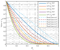
(a) AFL with different $\gamma$.

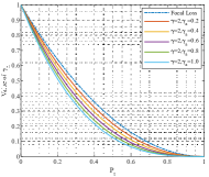
(b) AFL with different $\gamma_{\mathrm{a}}$.

Figure 8: The variation of $\gamma_{\mathrm{d}}$ at different values of the proposed AFL. In Fig. 8(a), to explore the effect of $\gamma$ on AFL, where $\gamma_{a}$ = 0.5. Similarly, in Fig. 8(b), $\gamma$ is set to $2$ to explore the effect of different values of $\gamma_{\mathrm{a}}$ on AFL.

(1) AFL allows the IIS model to focus more on low-confidence easy samples. As in Fig. 8(a), the AFL allows pixels with smaller $P^{i}_{t}$ to obtain higher gradient values for the same value of $\gamma$ compared with Focal Loss [37];

(2) AFL allows models to adaptively switch learning strategies. As in Fig. 8(b), compared to the rigid learning strategy of Focal Loss [37], AFL is more flexible in its learning style. When faced with samples with significant differences in pixel difficulty distributions, the value of $\gamma_{\mathrm{d}}$ will be increased to overcome inadequate learning. Conversely, when facing samples with minor differences, the proposed $\gamma_{\mathrm{d}}$ can adopt a small value to overcome over-learning (over-fitting) of extremely difficult pixels.

References

- [1] J. Wu, Y. Zhao, J.-Y. Zhu, S. Luo, and Z. Tu, “MILCut: A sweeping line multiple instance learning paradigm for interactive image segmentation,” in CVPR, 2014, pp. 256–263.
- [2] M. Jian and C. Jung, “Interactive image segmentation using adaptive constraint propagation,” TIP, vol. 25, no. 3, pp. 1301–1311, 2016.
- [3] T. Wang, J. Yang, Z. Ji, and Q. Sun, “Probabilistic diffusion for interactive image segmentation,” TIP, vol. 28, no. 1, pp. 330–342, 2018.
- [4] D. Galeev, P. Popenova, A. Vorontsova, and A. Konushin, “Contour-based interactive segmentation,” arXiv preprint arXiv:2302.06353, 2023.
- [5] T. Wang, Z. Ji, J. Yang, Q. Sun, and P. Fu, “Global manifold learning for interactive image segmentation,” TMM, vol. 23, pp. 3239–3249, 2020.
- [6] X. Chen, Y. S. J. Cheung, S.-N. Lim, and H. Zhao, “Scribbleseg: Scribble-based interactive image segmentation,” arXiv preprint arXiv:2303.11320, 2023.
- [7] M. Jian and C. Jung, “Interactive image segmentation using adaptive constraint propagation,” TIP, vol. 25, no. 3, pp. 1301–1311, 2016.
- [8] K. Sofiiuk, I. A. Petrov, and A. Konushin, “Reviving iterative training with mask guidance for interactive segmentation,” in ICIP, 2022, pp. 3141–3145.
- [9] Q. Liu et al., “PseudoClick: Interactive image segmentation with click imitation,” in ECCV, 2022, pp. 728–745.
- [10] Z. Lin, Z.-P. Duan, Z. Zhang, C.-L. Guo, and M.-M. Cheng, “FocusCut: Diving into a focus view in interactive segmentation,” in CVPR, 2022, pp. 2637–2646.
- [11] G. Wang et al., “DeepIGeoS: A deep interactive geodesic framework for medical image segmentation,” TPAMI, vol. 41, no. 7, pp. 1559–1572, 2019.
- [12] A. Diaz-Pinto et al., “DeepEdit: Deep editable learning for interactive segmentation of 3D medical images,” in MICCAI, 2022, pp. 11–21.
- [13] C. Ma et al., “Boundary-aware supervoxel-level iteratively refined interactive 3D image segmentation with multi-agent reinforcement learning,” TMI, vol. 40, no. 10, pp. 2563–2574, 2020.
- [14] J. Deng and X. Xie, “3D interactive segmentation with semi-implicit representation and active learning,” TIP, vol. 30, pp. 9402–9417, 2021.
- [15] D. Henghui, Z. Hui, L. Chang, and J. Xudong, “Deep interactive image matting with feature propagation,” TIP, vol. 31, pp. 2421–2432, 2022.
- [16] H. Ding, H. Zhang, C. Liu, and X. Jiang, “Deep interactive image matting with feature propagation,” TIP, vol. 31, pp. 2421–2432, 2022.
- [17] Z. Lin, Z. Zhang, L.-Z. Chen, M.-M. Cheng, and S.-P. Lu, “Interactive image segmentation with first click attention,” in CVPR, 2020, pp. 13 339–13 348.
- [18] S. Majumder and A. Yao, “Content-aware multi-level guidance for interactive instance segmentation,” in CVPR, 2019, pp. 11 602–11 611.
- [19] X. Chen, Z. Zhao, F. Yu, Y. Zhang, and M. Duan, “Conditional diffusion for interactive segmentation,” in ICCV, 2021, pp. 7345–7354.
- [20] Z. Li, Q. Chen, and V. Koltun, “Interactive image segmentation with latent diversity,” in CVPR, 2018, pp. 577–585.
- [21] J. H. Liew, S. Cohen, B. Price, L. Mai, S.-H. Ong, and J. Feng, “MultiSeg: Semantically meaningful, scale-diverse segmentations from minimal user input,” in ICCV, 2019, pp. 662–670.
- [22] Z. Ding, T. Wang, Q. Sun, and F. Chen, “Rethinking click embedding for deep interactive image segmentation,” TII, vol. 19, no. 1, pp. 261–273, 2023.
- [23] X. Chen, Z. Zhao, Y. Zhang, M. Duan, D. Qi, and H. Zhao, “FocalClick: Towards practical interactive image segmentation,” in CVPR, 2022, pp. 1300–1309.
- [24] Q. Liu, Z. Xu, Y. Jiao, and M. Niethammer, “iSegFormer: Interactive segmentation via transformers with application to 3D knee MR images,” in MICCAI, 2022, pp. 464–474.
- [25] W.-D. Jang and C.-S. Kim, “Interactive image segmentation via backpropagating refinement scheme,” in CVPR, 2019, pp. 5297–5306.
- [26] K. Sofiiuk, I. Petrov, O. Barinova, and A. Konushin, “F-BRS: Rethinking backpropagating refinement for interactive segmentation,” in CVPR, 2020, pp. 8623–8632.
- [27] N. Xu, B. Price, S. Cohen, J. Yang, and T. S. Huang, “Deep interactive object selection,” in CVPR, 2016, pp. 373–381.
- [28] Q. Liu, Z. Xu, G. Bertasius, and M. Niethammer, “SimpleClick: Interactive image segmentation with simple vision transformers,” arXiv preprint arXiv:2210.11006, 2022.
- [29] Q. Wei, H. Zhang, and J.-H. Yong, “Focused and collaborative feedback integration for interactive image segmentation,” arXiv preprint arXiv:2303.11880, 2023.
- [30] A. Kirillov et al., “Segment anything,” arXiv preprint arXiv:2304.02643, 2023.
- [31] Y. Huang et al., “InterFormer: Real-time interactive image segmentation,” 2023.
- [32] A. Rana, S. Mahadevan, A. Hermans, and B. Leibe, “DynaMITe: Dynamic query bootstrapping for multi-object interactive segmentation transformer,” arXiv preprint arXiv:2304.06668, 2023.
- [33] X. Zou, J. Yang, H. Zhang, F. Li, L. Li, J. Gao, and Y. J. Lee, “Segment everything everywhere all at once,” arXiv preprint arXiv:2304.06718, 2023.
- [34] J. Liew, Y. Wei, W. Xiong, S.-H. Ong, and J. Feng, “Regional interactive image segmentation networks,” in ICCV, 2017, pp. 2746–2754.
- [35] R. Benenson, S. Popov, and V. Ferrari, “Large-scale interactive object segmentation with human annotators,” in CVPR, 2019, pp. 11 700–11 709.
- [36] M. Forte, B. Price, S. Cohen, N. Xu, and F. Pitié, “Getting to 99% accuracy in interactive segmentation,” arXiv preprint arXiv:2003.07932, 2020.
- [37] T.-Y. Lin, P. Goyal, R. Girshick, K. He, and P. Dollár, “Focal loss for dense object detection,” in ICCV, 2017, pp. 2980–2988.
- [38] A. Dosovitskiy et al., “An image is worth 16x16 words: Transformers for image recognition at scale,” in ICLR, 2021.
- [39] T. Kontogianni, M. Gygli, J. Uijlings, and V. Ferrari, “Continuous adaptation for interactive object segmentation by learning from corrections,” in ECCV, 2020, pp. 579–596.
- [40] T. Brown et al., “Language models are few-shot learners,” in NeurIPS, vol. 33, 2020, pp. 1877–1901.
- [41] B. Cheng, I. Misra, A. G. Schwing, A. Kirillov, and R. Girdhar, “Masked-attention mask transformer for universal image segmentation,” in CVPR, 2022, pp. 1290–1299.
- [42] M. Yi-de, L. Qing, and Q. Zhi-Bai, “Automated image segmentation using improved pcnn model based on cross-entropy,” in ISIMVSP, 2004, pp. 743–746.
- [43] Z. Leng et al., “PolyLoss: A polynomial expansion perspective of classification loss functions,” in ICLR, 2022.
- [44] V. Pihur, S. Datta, and S. Datta, “Weighted rank aggregation of cluster validation measures: a monte carlo cross-entropy approach,” Bioinformatics, vol. 23, no. 13, pp. 1607–1615, 2007.
- [45] S. Xie and Z. Tu, “Holistically-nested edge detection,” in ICCV, 2015, pp. 1395–1403.
- [46] B. Li et al., “Equalized focal loss for dense long-tailed object detection,” in CVPR, 2022, pp. 6990–6999.
- [47] K.-K. Maninis, S. Caelles, J. Pont-Tuset, and L. Van Gool, “Deep extreme cut: From extreme points to object segmentation,” in CVPR, 2018, pp. 616–625.
- [48] S. Majumder and A. Yao, “Content-aware multi-level guidance for interactive instance segmentation,” in CVPR, 2019, pp. 11 602–11 611.
- [49] M. A. Rahman and Y. Wang, “Optimizing intersection-over-union in deep neural networks for image segmentation,” in ISVC, 2016, pp. 234–244.
- [50] F. Milletari, N. Navab, and S.-A. Ahmadi, “V-net: Fully convolutional neural networks for volumetric medical image segmentation,” in 3DV, 2016, pp. 565–571.
- [51] S. Jadon, “A survey of loss functions for semantic segmentation,” in CIBCB, 2020, pp. 1–7.
- [52] K. Sofiiuk, O. Barinova, and A. Konushin, “AdaptIS: Adaptive instance selection network,” in ICCV, 2019, pp. 7355–7363.
- [53] M. Zhou et al., “Interactive segmentation as gaussian process classification,” arXiv preprint arXiv:2302.14578, 2023.
- [54] T.-Y. Lin, P. Dollár, R. Girshick, K. He, B. Hariharan, and S. Belongie, “Feature pyramid networks for object detection,” in CVPR, 2017, pp. 2117–2125.
- [55] X. Zhu, W. Su, L. Lu, B. Li, X. Wang, and J. Dai, “DD deformable transformers for end-to-end object detection,” in ICLR, 2021, pp. 3–7.
- [56] A. Botach, E. Zheltonozhskii, and C. Baskin, “End-to-end referring video object segmentation with multimodal transformers,” in CVPR, 2022, pp. 4985–4995.
- [57] B. Cheng, A. Schwing, and A. Kirillov, “Per-pixel classification is not all you need for semantic segmentation,” in NeurIPS, vol. 34, 2021, pp. 17 864–17 875.
- [58] N. Carion, F. Massa, G. Synnaeve, N. Usunier, A. Kirillov, and S. Zagoruyko, “End-to-end object detection with transformers,” in ECCV, 2020, pp. 213–229.
- [59] W. Rudin et al., Principles of mathematical analysis. McGraw-hill New York, 1976, vol. 3.
- [60] H. P. Heinig and L. Maligranda, “Chebyshev inequality in function spaces,” Real Analysis Exchange, pp. 211–247, 1991.
- [61] T.-Y. Lin et al., “Microsoft COCO: Common objects in context,” in ECCV, 2014, pp. 740–755.
- [62] A. Gupta, P. Dollar, and R. Girshick, “LVIS: A dataset for large vocabulary instance segmentation,” in CVPR, 2019, pp. 5356–5364.
- [63] C. Rother, V. Kolmogorov, and A. Blake, ““GrabCut” interactive foreground extraction using iterated graph cuts,” ACM Trans. Graph., vol. 23, no. 3, pp. 309–314, 2004.
- [64] K. McGuinness and N. E. O’connor, “A comparative evaluation of interactive segmentation algorithms,” PR, vol. 43, no. 2, pp. 434–444, 2010.
- [65] F. Perazzi, J. Pont-Tuset, B. McWilliams, L. Van Gool, M. Gross, and A. Sorkine-Hornung, “A benchmark dataset and evaluation methodology for video object segmentation,” in CVPR, 2016, pp. 724–732.
- [66] M. Everingham, L. Van Gool, C. K. Williams, J. Winn, and A. Zisserman, “The pascal visual object classes (VOC) challenge,” IJCV, vol. 88, no. 2, pp. 303–338, 2010.
- [67] S. Gerhard, J. Funke, J. Martel, A. Cardona, and R. Fetter, “Segmented anisotropic ssTEM dataset of neural tissue,” Figshare, pp. 0–0, 2013.
- [68] U. Baid et al., “The RSNA-ASNR-MICCAI BraTS 2021 benchmark on brain tumor segmentation and radiogenomic classification,” arXiv preprint arXiv:2107.02314, 2021.
- [69] F. Ambellan, A. Tack, M. Ehlke, and S. Zachow, “Automated segmentation of knee bone and cartilage combining statistical shape knowledge and convolutional neural networks: Data from the osteoarthritis initiative,” Med Image Anal., vol. 52, pp. 109–118, 2019.
- [70] Y. Li, H. Mao, R. Girshick, and K. He, “Exploring plain vision transformer backbones for object detection,” in ECCV, 2022, pp. 280–296.
- [71] K. He, X. Chen, S. Xie, Y. Li, P. Dollár, and R. Girshick, “Masked autoencoders are scalable vision learners,” in CVPR, 2022, pp. 16 000–16 009.
- [72] J. Deng, W. Dong, R. Socher, L.-J. Li, K. Li, and L. Fei-Fei, “ImageNet: A large-scale hierarchical image database,” in CVPR, 2009, pp. 248–255.
- [73] Y. Hao et al., “EdgeFlow: Achieving practical interactive segmentation with edge-guided flow,” in ICCV, 2021, pp. 1551–1560.
- [74] M. Antonelli et al., “The medical segmentation decathlon,” Nat. Commun., vol. 13, no. 1, p. 4128, 2022.
- [75] G. Feng, Z. Hu, L. Zhang, J. Sun, and H. Lu, “Bidirectional relationship inferring network for referring image localization and segmentation,” TNNLS, vol. 34, no. 5, pp. 2246–2258, 2023.
- [76] G. Feng, L. Zhang, Z. Hu, and H. Lu, “Learning from box annotations for referring image segmentation,” TNNLS, pp. 1–11, 2022.