Maximization of Nonsubmodular Functions under Multiple Constraints with Applications

Abstract

We consider the problem of maximizing a monotone nondecreasing set function under multiple constraints, where the constraints are also characterized by monotone nondecreasing set functions. We propose two greedy algorithms to solve the problem with provable approximation guarantees. The first algorithm exploits the structure of a special class of the general problem instance to obtain a better time complexity. The second algorithm is suitable for the general problem. We characterize the approximation guarantees of the two algorithms, leveraging the notions of submodularity ratio and curvature introduced for set functions. We then discuss particular applications of the general problem formulation to problems that have been considered in the literature. We validate our theoretical results using numerical examples.

, , , ,

1 Introduction

We study the problem of maximizing a set function over a ground set $\mathcal{S}$ in the presence of $n$ constraints, where the constraints are also characterized by set functions. Specifically, given monotone nondecreasing set functions $f:2^{\mathcal{S}}\to\mathbb{R}_{\geq 0}$ and $h_{i}:2^{\mathcal{S}}\to\mathbb{R}_{\geq 0}$ for all $i\in[n]\triangleq\{1,\dots,n\}$ with $n\in\mathbb{Z}_{\geq 1}$, we consider the following constrained optimization problem:

$$\begin{split}&\max_{\mathcal{A}\subseteq\mathcal{S}}f(\mathcal{A})\\ &s.t.\ h_{i}(\mathcal{A}\cap\mathcal{S}_{i})\leq H_{i},\ \forall i\in[n],\end{split}$$ (P1)

where $\mathcal{S}=\cup_{i\in[n]}\mathcal{S}_{i}$, with $\mathcal{S}_{i}\subseteq\mathcal{S}$ for all $i\in[n]$, and $H_{i}\in\mathbb{R}_{\geq 0}$ for all $i\in[n]$. By simultaneously allowing nonsubmodular set functions (in both the objective and the constraints) and multiple constraints (given by upper bounds on the set functions), (P1) generalizes a number of combinatorial optimization problems (e.g., [20, 17, 25, 24, 3, 9]). Instances of (P1) arise in many important applications, including sensor (or measurement) selection for state (or parameter) estimation (e.g., [18, 40, 37]), experimental design (e.g., [22, 3]), and data subset (or client) selection for machine learning (e.g., [8, 11, 36]). As an example, the problem of sensor selection for minimizing the error covariance of the Kalman filter (studied, e.g., in [18, 39]) can be viewed as a special case of (P1) where the objective function $f(\cdot)$ is defined on the ground set $\mathcal{S}$ that contains all candidate sensors, and is used to characterize the state estimation performance of the Kalman filter using measurements from an allowed set $\mathcal{A}\subseteq\mathcal{S}$ of selected sensors. The constraints corresponding to $h_{i}(\cdot)$ for all $i\in[n]$ represent, e.g., budget, communication, spatial and energy constraints on the set of selected sensors (e.g., [28, 39, 31]). We apply our results to two specific problems in Section 4.

In general, (P1) is NP-hard (e.g., [13]), i.e., obtaining an optimal solution to (P1) is computationally expensive. For instances of (P1) with a monotone nondecreasing submodular objective function $f(\cdot)$ and a single constraint, there is a long line of work for showing that greedy algorithms yield constant-factor approximation ratios for (P1) (e.g., [29, 20, 4]). However, many important applications that can be captured by the general problem formulation in (P1) do not feature objective functions that are submodular (see, e.g., [22, 8, 40, 12, 39]). For instances of (P1) with a nonsubmodular objective function $f(\cdot)$, it has been shown that the greedy algorithms yield approximation ratios that depend on the problem parameters (e.g., [8, 3, 34]). As an example, the approximation ratio of the greedy algorithm provided in [3] depends on the submodularity ratio and the curvature of the objective function in (P1).

Moreover, most of the existing works consider instances of (P1) with a single constraint on the set of the selected elements, e.g., a cardinality, budget, or a matroid constraint. The objective of this paper is to relax this requirement of a single simple constraint being present on the set of selected elements. For instance, in the Kalman filtering based sensor scheduling (or selection) problem described above, a natural formulation is to impose a separate constraint on the set of sensors selected at different time steps, or to consider multiple constraints such as communication and budget constraints on how many sensors can work together simultaneously. Thus, we consider the problem formulation (P1), where the objective function is a monotone nondecreasing set function and the constraints are also characterized by monotone nondecreasing set functions. We do not assume that the objective function and the functions in the constraints are necessarily submodular. We propose approximation algorithms to solve (P1), and provide theoretical approximation guarantees for the proposed algorithms leveraging the notions of curvature and submodularity ratio.

Our main contributions are summarized as follows. First, we consider instances of (P1) with $\mathcal{S}_{i}\cap\mathcal{S}_{j}=\emptyset$ for all $i,j\in[n]$ ($i\neq j$), and propose a parallel greedy algorithm with time complexity $O((\max_{i\in[n]}|\mathcal{S}_{i}|)^{2})$ that runs for each $i\in[n]$ in parallel. We characterize the approximation guarantee of the parallel greedy algorithm, leveraging the submodularity and curvature of the set functions in the instances of (P1). Next, we consider general instances of (P1) without utilizing the assumption on mutually exclusive sets $S_{i}$. We propose a greedy algorithm with time complexity $O(n|\mathcal{S}|^{2})$, and characterize its approximation guarantee. The approximation guarantee of this algorithm again depends on the submodularity ratio and curvature of the set functions and the solution returned by the algorithm. Third, we specialize these results to some example applications and evaluate these approximation guarantees by bounding the submodularity ratio and curvature of the set functions. Finally, we validate our theoretical results using numerical examples; the results show that the two greedy algorithms yield comparable performances that are reasonably good in practice. A preliminary version of this paper was presented in [36], where only the parallel greedy algorithm was studied for a special instance of (P1).

Notation For a matrix $P\in\mathbb{R}^{n\times n}$, let $P^{\top}$, $\text{Tr}(P)$, $\lambda_{1}(P)$ and $\lambda_{n}(P)$ be its transpose, trace, an eigenvalue with the largest magnitude, and an eigenvalue with the smallest magnitude, respectively. A positive definite matrix $P\in\mathbb{R}^{n\times n}$ is denoted by $P\succ 0$. Let $I_{n}$ denote an $n\times n$ identity matrix. For a vector $x$, let $x_{i}$ (or $(x)_{i}$) be the $i$th element of $x$, and define $\textrm{supp}(x)=\{i:x_{i}\neq 0\}$. The Euclidean norm of $x$ is denoted by $\lVert x\rVert$. Given two functions $\varphi_{1}:\mathbb{R}_{\geq 0}\to\mathbb{R}$ and $\varphi_{2}:\mathbb{R}_{\geq 0}\to\mathbb{R}$, $\varphi_{1}(n)$ is $O(\varphi_{2}(n))$ if there exist positive constants $c$ and $N$ such that $|\varphi_{1}(n)|\leq c|\varphi_{2}(n)|$ for all $n\geq N$.

2 Preliminaries

We begin with some definitions (see, e.g.,[29, 7, 3, 23]).

Definition 1.

The submodularity ratio of $h:2^{\mathcal{S}}\to\mathbb{R}_{\geq 0}$ is the largest $\gamma\in\mathbb{R}$ such that

$$\sum_{v\in\mathcal{A}\setminus\mathcal{B}}\big{(}h(\{v\}\cup\mathcal{B})-h(\mathcal{B})\big{)}\geq\gamma\big{(}h(\mathcal{A}\cup\mathcal{B})-h(\mathcal{B})\big{)},$$ (1)

for all $A,B\subseteq\mathcal{S}$. The diminishing return (DR) ratio of $h(\cdot)$ is the largest $\kappa\in\mathbb{R}$ such that

$$h(\mathcal{A}\cup\{v\})-h(\mathcal{A})\geq\kappa\big{(}h(\mathcal{B}\cup\{v\})-h(\mathcal{B})\big{)},$$ (2)

for all $\mathcal{A}\subseteq\mathcal{B}\subseteq\mathcal{S}$ and for all $v\in\mathcal{S}\setminus\mathcal{B}$.

Definition 2.

The curvature of $h:2^{\mathcal{S}}\to\mathbb{R}_{\geq 0}$ is the smallest $\alpha\in\mathbb{R}$ that satisfies

$$h(\mathcal{A}\cup\{v\})-h(\mathcal{A})\geq(1-\alpha)\big{(}h(\mathcal{B}\cup\{v\})-h(\mathcal{B})\big{)},$$ (3)

for all $\mathcal{B}\subseteq\mathcal{A}\subseteq\mathcal{S}$ and for all $v\in\mathcal{S}\setminus\mathcal{A}$. The extended curvature of $h(\cdot)$ is the smallest $\tilde{\alpha}\in\mathbb{R}$ that satisfies

$$h(\mathcal{A}\cup\{v\})-h(\mathcal{A})\geq(1-\tilde{\alpha})\big{(}h(\mathcal{B}\cup\{v\})-h(\mathcal{B})\big{)},$$ (4)

for all $\mathcal{A},\mathcal{B}\subseteq\mathcal{S}$ and for all $v\in(\mathcal{S}\setminus\mathcal{A})\cap(\mathcal{S}\setminus\mathcal{B})$.

For any monotone nondecreasing set function $h:2^{\mathcal{S}}\to\mathbb{R}_{\geq 0}$, one can check that the submodularity ratio $\gamma$, the DR ratio $\kappa$, the curvature $\alpha$ and the extended curvature $\tilde{\alpha}$ of $h(\cdot)$ satisfy that $\gamma,\kappa,\alpha,\tilde{\alpha}\in[0,1]$. Moreover, we see from Definition 2 that $\tilde{\alpha}\geq\alpha$, and it can also been shown that $\gamma\geq\kappa$ (e.g., [3, 23, 36]). Further assuming that $h(\cdot)$ is submodular, one can show that $\gamma=\kappa=1$ (e.g., [3, 23]). For a modular set function $h:2^{\mathcal{S}}\to\mathbb{R}_{\geq 0}$, we see from Definition 2 that the curvature and the extended curvature of $h(\cdot)$ satisfy that $\alpha=\tilde{\alpha}=0$. Thus, the submodularity (resp., DR) ratio of a monotone nondecreasing set function $h(\cdot)$ characterizes the approximate submodularity (resp., approximate DR property) of $h(\cdot)$. The curvatures of $h(\cdot)$ characterize how far the function $h(\cdot)$ is from being modular. Before we proceed, we note that the set $\mathcal{S}_{i}$ in (P1) can potentially intersect with $\mathcal{S}_{j}$, for any $i,j\in\mathcal{S}$ with $i\neq j$. Moreover, one can show that a cardinality constraint, a (partitioned) matroid constraint, or multiple budget constraints on the set $\mathcal{A}$ of selected elements are special cases of the constraints in (P1). In particular, $h_{i}(\cdot)$ in (P1) reduces to a modular set function for any $i\in[n]$ when considering budget constraints.

3 Approximation Algorithms

We make the following standing assumption.

Assumption 3.

The set functions $f(\cdot)$ and $h_{i}(\cdot)$ satisfy that $f(\emptyset)=0$ and $h_{i}(\emptyset)=0$ for all $i\in[n]$. Further, $h_{i}(v)>0$ for all $i\in[n]$ and for all $v\in\mathcal{S}$.

Note that (P1) is NP-hard, and cannot be approximated within any constant factor independent of all problem parameters (if P$\neq$NP), even when the constraints in (P1) reduce to a cardinality constraint $|\mathcal{A}|\leq H$ [39]. Thus, we aim to provide approximation algorithms for (P1) and characterize the corresponding approximation guarantees in terms of the problem parameters. To simplify the notation in the sequel, for any $\mathcal{A},\mathcal{B}\subseteq\mathcal{S}$, we denote

$$\begin{split}&\delta_{\mathcal{B}}(\mathcal{A})=f(\mathcal{A}\cup\mathcal{B})-f(\mathcal{A})\\ &\delta_{\mathcal{B}}^{i}(\mathcal{A})=h_{i}(\mathcal{A}\cup\mathcal{B}\cap\mathcal{S}_{i})-h_{i}(\mathcal{A}\cap\mathcal{S}_{i}).\end{split}$$ (5)

Thus, $\delta_{\mathcal{B}}(\mathcal{A})$ (resp., $\delta_{\mathcal{B}}^{i}(\mathcal{A})$) is the marginal return of $f(\cdot)$ (resp., $h_{i}(\cdot)$) when adding $\mathcal{B}$ to $\mathcal{A}$.

3.1 Parallel Greedy Algorithm for a Special Case

We rely on the following assumption and introduce a parallel greedy algorithm (Algorithm 1) for (P1).

Assumption 4.

The ground set $\mathcal{S}=\cup_{i\in[n]}\mathcal{S}_{i}$ in (P1) satisfies that $\mathcal{S}_{i}\cap\mathcal{S}_{j}=\emptyset$ for all $i,j\in[n]$ with $i\neq j$.

Input: $\mathcal{S}=\cup_{i\in[n]}\mathcal{S}_{i}$, $f:2^{\mathcal{S}}\to\mathbb{R}_{\geq 0}$ and $h_{i}:2^{\mathcal{S}}\to\mathbb{R}_{\geq 0}$ $\forall i\in[n]$, $H_{i}\in\mathbb{R}_{\geq 0}$ $\forall i\in[n]$

Algorithm 1 Parallel greedy algorithm

1:for each $i\in[n]$ in parallel do

2:     $\mathcal{W}_{i}\leftarrow\mathcal{S}_{i}$, $\mathcal{A}_{i}^{r}\leftarrow\emptyset$

3:     $\mathcal{B}_{i}^{r}\leftarrow\arg\max_{v\in\mathcal{S}_{i}}f(v)$

4:     while $\mathcal{W}_{i}\neq\emptyset$ do

5:         $v^{\star}\leftarrow\arg\max_{v\in\mathcal{W}_{i}}\frac{\delta_{v}(\mathcal{A}_{i}^{r})}{\delta_{v}^{i}(\mathcal{A}_{i}^{r})}$

6:         if $h_{i}(\mathcal{A}_{i}^{r}\cup\{v^{\star}\})\leq H_{i}$ then

7:              $\mathcal{A}_{i}^{r}\leftarrow\mathcal{A}_{i}^{r}\cup\{v^{\star}\}$          

8:         $\mathcal{W}_{i}\leftarrow\mathcal{W}_{i}\setminus\{v^{\star}\}$      

9:     $\mathcal{A}_{i}^{r}\leftarrow\arg\max_{\mathcal{A}\in\{\mathcal{A}_{i}^{r},\mathcal{B}_{i}^{r}\}}f(\mathcal{A})$

10:$\mathcal{A}^{r}\leftarrow\cup_{i\in[n]}\mathcal{A}_{i}^{r}$

11:Return $\mathcal{A}^{r}$

For each $i\in[n]$ in parallel, Algorithm 1 first sets $\mathcal{S}_{i}$ to be the ground set $\mathcal{W}_{i}$ for the algorithm, and then iterates over the current elements in $\mathcal{W}_{i}$ in the while loop. In particular, the algorithm greedily chooses an element $v\in\mathcal{W}_{i}$ in line 5 that maximizes the ratio between the marginal returns $\delta_{v}(\mathcal{A}_{i}^{r})$ and $\delta_{v}^{i}(\mathcal{A}_{i}^{r})$ for all $v\in\mathcal{W}_{i}$. The overall greedy solution is given by $\mathcal{A}^{r}=\cup_{i\in[n]}\mathcal{A}^{r}_{i}$. Thus, one may view Algorithm 1 as solving the problem $\max_{\mathcal{A}\subseteq\mathcal{S}_{i}}f(\mathcal{A})$ s.t. $h_{i}(\mathcal{A})\leq H_{i}$ for each $i\in[n]$ separately in parallel, and then merge the obtained solutions. Note that the overall time complexity of Algorithm 1 is $O((\max_{i\in[n]}|\mathcal{S}_{i}|)^{2})$. To provide a guarantee on the quality of the approximation for the solution returned by Algorithm 1, we start with the following observation, which follows directly from the definition of the algorithm.

Observation 1.

For any $i\in[n]$ in Algorithm 1, denote $\mathcal{A}_{i}^{r}=\{q_{1},\dots,q_{|\mathcal{A}_{i}^{r}|}\}$ and $\mathcal{A}_{i,j}^{r}=\{q_{1},\dots,q_{j}\}$ for all $j\in[|\mathcal{A}_{i}^{r}|]$ with $\mathcal{A}_{i,0}^{r}=\emptyset$. Then, there exists $l_{i}\in[|\mathcal{A}_{i}^{r}|]$ such that (1) $q_{k}\in\arg\max_{v\in\mathcal{W}_{i}}\frac{\delta_{v}(\mathcal{A}^{r}_{i,k-1})}{\delta_{v}^{i}(\mathcal{A}_{i,k-1}^{r})}$ and $h_{i}(\mathcal{A}_{i,k}^{r})\leq H_{i}$ for all $k\in[l_{i}]$; and (2) $h_{i}(\mathcal{A}_{i,l_{i}}^{r}\cup\{v^{\star}_{l_{i}+1}\})>H_{i}$, where $v^{\star}_{l_{i}+1}\in\arg\max_{v\in\mathcal{W}_{i}}\frac{\delta_{v}(\mathcal{A}_{i,l_{i}}^{r})}{\delta_{v}^{i}(\mathcal{A}_{i,l_{i}}^{r})}$.

Definition 5.

The greedy submodularity ratio of $f:2^{\mathcal{S}}\to\mathbb{R}_{\geq 0}$ in (P1) is the largest $\tilde{\gamma}_{f}\in\mathbb{R}$ that satisfies $f(\mathcal{B}_{i}^{r})\geq\tilde{\gamma}_{f}\big{(}f(\mathcal{A}_{i,l_{i}}^{r}\cup\{v_{l_{i}+1}^{\star}\})-f(\mathcal{A}_{i,l_{i}}^{r})\big{)}$ for all $i\in[n]$, where $v_{l_{i}+1}^{\star},\mathcal{A}_{i,l_{i}}^{r}$ are given in Observation 1, and $\mathcal{B}_{i}^{r}$ is given by line 3 of Algorithm 1.

For monotone nondecreasing $f(\cdot)$ in (P1), one can check that the greedy submodularity ratio of $f(\cdot)$ satisfies $\tilde{\gamma}_{f}\in\mathbb{R}_{\geq 0}$. Further assuming that $f(\cdot)$ is submodular, one can show that $\tilde{\gamma}_{f}\in\mathbb{R}_{\geq 1}$.

Theorem 6.

Suppose that Assumption 4 holds. Let $\mathcal{A}^{r}$ and $\mathcal{A}^{\star}$ be the solution to (P1) returned by Algorithm 1 and an optimal solution to (P1), respectively. Then,

$$f(\mathcal{A}^{r})\geq\frac{(1-\alpha_{f})\kappa_{f}\min\{1,\tilde{\gamma}_{f}\}}{2}\\ \times\min_{i\in[n]}(1-e^{-(1-\tilde{\alpha}_{i})\gamma_{f}})f(\mathcal{A}^{\star}),$$ (6)

where $\alpha_{f},\kappa_{f},\gamma_{f}\in[0,1]$ and $\tilde{\gamma}_{f}\in\mathbb{R}_{\geq 0}$ are the curvature, DR ratio, submodularity ratio and greedy submodularity ratio of $f(\cdot)$, respectively, and $\tilde{\alpha}_{i}\in[0,1]$ is the extended curvature of $h_{i}(\cdot)$ for all $i\in[n]$.

We briefly explain the ideas for the proof of Theorem 6; a detailed proof is included in Appendix A. Supposing that $h_{i}(\cdot)$ is modular for any $i\in[n]$, the choice $v^{\star}$ in line 5 of the algorithm reduces to $v^{\star}\leftarrow\arg\max_{v\in\mathcal{W}_{i}}\frac{\delta_{v}(\mathcal{A}_{i}^{r})}{h_{i}(v)}$, which is an element $v\in\mathcal{W}_{i}$ that maximizes the marginal return of the objective function $f(\cdot)$ per unit cost incurred by $h_{i}(\cdot)$ when adding $v$ to the current greedy solution $\mathcal{A}_{i}^{r}$. This renders the greedy nature of the choice $v^{\star}$. To leverage this greedy choice property when $h_{i}(\cdot)$ is not modular, we use the (extended) curvature of $h_{i}(\cdot)$ (i.e., $\tilde{\alpha}_{i}$) to measure how close $h_{i}(\cdot)$ is to being modular. Moreover, we use $\gamma_{f},\tilde{\gamma}_{f}$ to characterize the approximate submodularity of $f(\cdot)$. Note that the multiplicative factor $(1-\alpha_{f})\kappa_{f}$ in (6) results from merging $\mathcal{A}_{i}^{r}$ for all $i\in[n]$ into $\mathcal{A}^{r}$ in line 10 of the algorithm.

Remark 7.

Under the stronger assumption that the objective function $f(\cdot)$ in (P1) can be written as $f(\mathcal{A})=\sum_{i\in[n]}f(\mathcal{A}\cap\mathcal{S}_{i})$, similar arguments to those in the proof of Theorem 6 can be used to show that $f(\mathcal{A}^{r})\geq\frac{\min\{1,\tilde{\gamma}_{f}\}}{2}\min_{i\in[n]}(1-e^{-(1-\tilde{\alpha}_{i})\gamma_{f}})f(\mathcal{A}^{\star})$.

3.2 A Greedy Algorithm for the General Case

We now introduce a greedy algorithm (Algorithm 2) for general instances of (P1). The algorithm uses the following definition for the feasible set associated with the constraints in (P1):

$$\mathcal{F}=\big{\{}\mathcal{A}\subseteq\mathcal{S}:h_{i}(\mathcal{A}\cap\mathcal{S}_{i})\leq H_{i},\forall i\in[n]\big{\}}.$$

In the absence of Assumption 4, Algorithm 2 lets $\mathcal{S}=\cup_{i\in[n]}\mathcal{S}_{i}$ be the ground set $\mathcal{W}$ in the algorithm. Algorithm 2 then iterates over the current elements in $\mathcal{W}$, and greedily chooses $v\in\mathcal{W}$ and $i\in[n]$ in line 3 such that the ratio between the marginal returns $\delta_{v}(\mathcal{A}^{g})$ and $\delta_{v}^{i}(\mathcal{A}^{g})$ are maximized for all $v\in\mathcal{W}$ and for all $i\in[n]$. The element $v^{\star}$ will be added to $\mathcal{A}^{r}$ if the constraint $h_{i}(\mathcal{A}^{g}\cup\{v^{\star}\})\leq H_{i}$ is not violated for any $i\in[n]$. Note that different from line 5 in Algorithm 1, the maximization in line 3 of Algorithm 2 is also taken with respect to $i\in[n]$. This is because we do not consider the set $\mathcal{S}_{i}$ and the constraint associated with $h_{i}(\cdot)$ for each $i\in[n]$ separately in Algorithm 2. One can check that the time complexity of Algorithm 2 is $O(n|\mathcal{S}|^{2})$. In order to characterize the approximation guarantee of Algorithm 2, we introduce the following definition.

Definition 8.

Let $\mathcal{A}^{g}=\{q_{1},\dots,q_{|\mathcal{A}^{g}|}\}$ and $\mathcal{A}^{\star}$ be the solution to (P1) returned by Algorithm 2 and an optimal solution to (P1), respectively. Denote $\mathcal{A}^{g}_{j}=\{q_{1},\dots,q_{j}\}$ for all $j\in[|\mathcal{A}^{g}|]$ with $\mathcal{A}^{g}_{0}=\emptyset$. For any $j\in\{0,\dots,|\mathcal{A}^{g}|-1\}$, the $j$th greedy choice ratio of Algorithm 2 is the largest $\psi_{j}\in\mathbb{R}$ that satisfies

$$\frac{\delta_{q_{j+1}}(\mathcal{A}_{j}^{g})}{\delta^{i_{j}}_{q_{j+1}}(\mathcal{A}^{g}_{j})}\geq\psi_{j}\frac{\delta_{v}(\mathcal{A}_{j}^{g})}{\delta_{v}^{i}(\mathcal{A}_{j}^{g})},$$ (7)

for all $v\in\mathcal{A}^{\star}\setminus\mathcal{A}_{j}^{g}$ and for all $i\in[n]$, where $i_{j}\in[n]$ is the index of the constraint in (P1) that corresponds to $q_{j+1}$ given by line 3 of Algorithm 2.

Note that $v^{\star}$ chosen in line 3 of Algorithm 2 is not added to the greedy solution $\mathcal{A}_{g}$ if the constraint in line 4 is violated. Thus, the greedy choice ratio $\psi_{j}$ given in Definition 8 is used to characterize the suboptimality of $q_{j+1}\in\mathcal{A}_{g}$ in terms of the maximization over $v\in\mathcal{W}$ and $i\in[n]$ in line 3 of the algorithm. Since both $f(\cdot)$ and $h_{i}(\cdot)$ for all $i\in[n]$ are monotone nondecreasing functions, Definition 8 implies that $\psi_{j}\in\mathbb{R}_{\geq 0}$ for all $j\in\{0,\dots,|\mathcal{A}^{g}|-1\}$. We also note that for any $j\in\{0,\dots,|\mathcal{A}^{g}|-1\}$, a lower bound on $\psi_{j}$ may be obtained by considering all $v\in\mathcal{S}\setminus\mathcal{A}_{j}^{g}$ (instead of $v\in\mathcal{A}^{\star}\setminus\mathcal{A}_{j}^{g}$) in Definition 8. Such lower bounds on $\psi_{j}$ for all $j\in\{0,\dots,|\mathcal{A}^{g}|-1\}$ can be computed in $O(n|\mathcal{S}|^{2})$ time and in parallel to Algorithm 2. The approximation guarantee for Algorithm 2 is provided in the following result proven in Appendix B.

Input: $\mathcal{S}=\cup_{i\in[n]}\mathcal{S}_{i}$, $f:2^{\mathcal{S}}\to\mathbb{R}_{\geq 0}$ and $h_{i}:2^{\mathcal{S}}\to\mathbb{R}_{\geq 0}$ $\forall i\in[n]$, $H_{i}\in\mathbb{R}_{\geq 0}$ $\forall i\in[n]$

Algorithm 2 Greedy algorithm for general instances of (P1)

1:$\mathcal{W}\leftarrow\mathcal{S}$, $\mathcal{A}^{g}\leftarrow\emptyset$

2:while $\mathcal{W}\neq\emptyset$ do

3:     $(v^{\star},i^{\star})\leftarrow\arg\max_{(v\in\mathcal{W},i\in[n])}\frac{\delta_{v}(\mathcal{A}^{g})}{\delta_{v}^{i}(\mathcal{A}^{g})}$

4:     if $(\mathcal{A}^{g}\cup\{v^{\star}\})\in\mathcal{F}$ then

5:         $\mathcal{A}^{g}\leftarrow\mathcal{A}^{g}\cup\{v^{\star}\}$      

6:     $\mathcal{W}\leftarrow\mathcal{W}\setminus\{v^{\star}\}$

7:Return $\mathcal{A}^{g}$

Theorem 9.

Let $\mathcal{A}^{g}$ and $\mathcal{A}^{\star}$ be the solution to (P1) returned by Algorithm 2 and an optimal solution to (P1), respectively. Then,

$$\begin{split}f(\mathcal{A}^{g})&\geq\Big{(}1-(1-\frac{B}{|\mathcal{A}^{g}|})^{|\mathcal{A}^{g}|}\Big{)}f(\mathcal{A}^{\star})\\ &\geq(1-e^{-B})f(\mathcal{A}^{\star})\end{split}$$ (8)

with $B\triangleq\frac{(1-\alpha_{h})\gamma_{f}}{\sum_{i\in[n]}H_{i}}\sum_{j=0}^{|\mathcal{A}^{g}|-1}\psi_{j}\delta^{i_{j}}_{q_{j+1}}(\mathcal{A}_{j}^{g})$, where $\gamma_{f}\in[0,1]$ is the submodularity ratio of $f(\cdot)$, $\alpha_{h}\triangleq\min_{i\in[n]}\tilde{\alpha}_{i}$ with $\tilde{\alpha}_{i}\in[0,1]$ to be the extended curvature of $h_{i}(\cdot)$ for all $i\in[n]$, $\psi_{j}\in\mathbb{R}_{\geq 0}$ is the $j$th greedy choice ratio of Algorithm 2 for all $j\in\{0,\dots,|\mathcal{A}^{g}|-1\}$, and $i_{j}\in[n]$ is the index of the constraint in (P1) that corresponds to $q_{j+1}$ given by line 3 of Algorithm 2.

Similarly to Theorem 6, we leverage the greedy choice property corresponding to line 3 of Algorithm 2 and the properties of $f(\cdot)$ and $h_{i}(\cdot)$. However, since Algorithm 2 considers the constraints associated with $h_{i}(\cdot)$ for all $i\in[n]$ simultaneously, the proof of Theorem 9 requires more care, and the approximation guarantee in (8) does not contain the multiplicative factor $(1-\alpha_{f})\kappa_{f}$.

Remark 10.

Similarly to Observation 1, there exists the maximum $l\in[|\mathcal{A}^{g}|]$ such that for any $q_{j}\in\mathcal{A}_{l}^{g}$, $q_{j}$ does not violate the condition in line 4 of Algorithm 2 when adding to the greedy solution $\mathcal{A}^{g}$. One can then show via Definition 8 that $\psi_{j-1}\geq 1$ for all $j\in[|\mathcal{A}^{g}_{l}|]$. Further assuming that Assumption 4 holds, one can follow the arguments in the proof of Theorem 9 and show that

$$\begin{split}f(\mathcal{A}^{g})&\geq\Big{(}1-(1-\frac{\tilde{B}}{|\mathcal{A}^{g}_{l}|})^{|\mathcal{A}^{g}_{l}|}\Big{)}f(\mathcal{A}^{\star})\\ &\geq(1-e^{-\tilde{B}})f(\mathcal{A}^{\star}),\end{split}$$ (9)

where $\tilde{B}\triangleq\frac{(1-\alpha_{h})\gamma_{f}}{\sum_{i\in[n]}H_{i}}\sum_{i\in[n]}h_{i}(\mathcal{A}^{g}_{l}\cap\mathcal{S}_{i})$.

3.3 Comparisons to Existing Results

Theorems 6 and 9 generalize several existing results in the literature. First, consider instances of (P1) with a single budget constraint, i.e., $h(\mathcal{A})=\sum_{v\in\mathcal{A}}h(v)\leq H$. We see from Definition 2 that the extended curvature of $h(\cdot)$ is $1$. It follows from Remark 7 that the approximation guarantee of Algorithm 1 provided in Theorem 6 reduces to $f(\mathcal{A}^{r})\geq\frac{\min\{1,\tilde{\gamma}_{f}\}}{2}(1-e^{-\gamma_{f}})f(\mathcal{A}^{\star})$, which matches with the approximation guarantee of the greedy algorithm provided in [37]. Further assuming that the objective function $f(\cdot)$ in (P1) is submodular, we have from Definitions 1 and 5 that $\gamma_{f}=1$ and $\tilde{\gamma}_{f}\geq 1$, and the approximation guarantee of Algorithm 1 further reduces to $f(\mathcal{A}^{r})\geq\frac{1}{2}(1-e^{-1})f(\mathcal{A}^{\star})$, which matches with the results in [20, 25].

Second, consider instances of (P1) with a single cardinality constraint $h(\mathcal{A})=|\mathcal{A}|\leq H$. From Definition 2, we obtain that the curvature of $h(\cdot)$ is $1$. It follows from Remark 10 that the approximation guarantee of Algorithm 2 provided in Theorem 9 reduces to $f(\mathcal{A}^{g})\geq(1-e^{-\gamma_{f}})f(\mathcal{A}^{\star})$, which matches with the approximation guarantee of the greedy algorithm provided in [9]. Further assuming that the objective function $f(\cdot)$ in (P1) is submodular, we see from Definition 1 that the approximation guarantee of Algorithm 2 reduces to $f(\mathcal{A}^{g})\geq(1-e^{-1})f(\mathcal{A}^{\star})$, which matches with the result in [29].

Third, consider instances of (P1) with a partitioned matroid constraint, i.e., $h_{i}(\mathcal{A}\cap\mathcal{S}_{i})=|\mathcal{A}\cap\mathcal{S}_{i}|\leq H_{i}$ $\forall i\in[n]$. Definition 2 shows that the curvature of $h_{i}(\cdot)$ is $1$ for all $i\in[n]$. Using similar arguments to those in Remark 10 and the proof of Theorem 9, one can show that Algorithm 2 yields the following approximation guarantee:

$$f(\mathcal{A}^{g})\geq\Big{(}1-(1-\frac{\gamma_{f}}{\sum_{i\in[n]}H_{i}})^{|\mathcal{A}^{g}_{l}|}\Big{)}f(\mathcal{A}^{\star}).$$ (10)

Further assuming that $f(\cdot)$ in (P1) is submodular, i.e., $\gamma_{f}=1$ in (10), one can check that the approximation guarantee in (10) matches with the result in [14].

4 Specific Application Settings

We now discuss some specific applications that can be captured by the general problem formulation in (P1). For these applications, we bound the parameters given by Definitions 1-2 and evaluate the resulting approximation guarantees provided in Theorems 6 and 9.

4.1 Sensor Selection

Sensor selection problems arise in many different applications, e.g., [22, 19, 6, 39]. A typical scenario is that only a subset of all candidate sensors can be used to estimate the state of a target environment or system. The goal is to select this subset to optimize an estimation performance metric. If the target system is a dynamical system whose state evolves over time, this problem is sometimes called sensor scheduling, in which different sets of sensors can be selected at different time steps (e.g., [18]) with possibly different constraints on the set of sensors selected at different time steps.

As an example, we can consider the Kalman filtering sensor scheduling (or selection) problem (e.g., [18, 35, 5, 39]) for a linear time-varying system

$$\begin{split}x_{k+1}&=A_{k}x_{k}+w_{k}\\ y_{k}&=C_{k}x_{k}+v_{k},\end{split}$$ (11)

where $A_{k}\in\mathbb{R}^{n\times n}$, $C_{k}\in\mathbb{R}^{m\times n}$, $x_{0}\sim\mathcal{N}(0,\Pi_{0})$ with $\Pi_{0}\succ 0$, $w_{k},v_{k}$ are zero-mean white Gaussian noise processes with $\mathbb{E}[w_{k}w_{k}^{\top}]=W\succ 0$, $\mathbb{E}[v_{k}v_{k}^{\top}]=\text{diag}(\sigma_{1}^{2}\cdots\sigma_{m}^{2})$, for all $k\in\mathbb{Z}_{\geq 0}$ with $\sigma_{i}>0$ for all $i\in[m]$, and $x_{0}$ is independent of $w_{k},v_{k}$ for all $k\in\mathbb{Z}_{\geq 0}$. If there are multiple sensors present, we can let each row in $C_{k}$ correspond to a candidate sensor at time step $k$. Given a target time step $\ell\in\mathbb{Z}_{\geq 0}$, we let $\mathcal{S}=\{(k,i):i\in[m],k\in\{0,\dots,\ell\}\}$ be the ground set that contains all the candidate sensors at different time steps. Thus, we can write $\mathcal{S}=\cup_{k\in\{0,\dots,\ell\}}\mathcal{S}_{k}$ with $\mathcal{S}_{k}=\{(k,i):i\in[m]\}$, where $\mathcal{S}_{k}$ (with $|\mathcal{S}_{k}|=m$) is the set of sensors available at time step $k$. Now, for any $\mathcal{A}_{k}\subseteq\mathcal{S}_{k}$, let $C_{\mathcal{A}_{k}}\in\mathbb{R}^{|\mathcal{A}_{k}|\times n}$ be the measurement matrix corresponding to the sensors in $\mathcal{A}_{k}$, i.e., $C_{\mathcal{A}_{k}}$ contains rows from $C_{k}$ that correspond to the sensors in $\mathcal{A}_{k}$. We then consider the following set function $g:2^{\mathcal{S}}\to\mathbb{R}_{\geq 0}$:

$$g(\mathcal{A})=\text{Tr}\Big{(}\big{(}P_{\ell,\mathcal{A}}^{-1}+\sum_{v\in\mathcal{A}_{\ell}}\sigma_{v}^{-2}C_{v}^{\top}C_{v}\big{)}^{-1}\Big{)},$$ (12)

where $\mathcal{A}=\cup_{k\in\{0,\dots,\ell\}}\mathcal{A}_{k}\subseteq\mathcal{S}$ with $\mathcal{A}_{k}\subseteq\mathcal{S}_{k}$, and $P_{\ell,\mathcal{A}}$ is given recursively via

$$P_{k+1,\mathcal{A}}=W+A_{k}\big{(}P_{k,\mathcal{A}}^{-1}+\sum_{v\in\mathcal{A}_{k}}\sigma_{v}^{-2}C_{v}^{\top}C_{v}\big{)}^{-1}A_{k}^{\top},$$ (13)

for $k=\{0,\dots,\ell-1\}$ with $P_{0,\mathcal{A}}=\Pi_{0}$. For any $\mathcal{A}\subseteq\mathcal{S}$, $g(\mathcal{A})$ is the mean square estimation error of the Kalman filter for estimating the system state $x_{\ell}$ based on the measurements (up until time step $\ell$) from the sensors in $\mathcal{A}$ (e.g., [1]). Thus, the sensor selection problem can be cast in the framework of (P1) as:

$$\begin{split}&\max_{\mathcal{A}\subseteq\mathcal{S}}\Big{\{}f_{s}(\mathcal{A})\triangleq g(\emptyset)-g(\mathcal{A})\Big{\}}\\ &\textrm{s.t.}\ h_{k}(\mathcal{A}\cap\mathcal{S}_{k})\leq H_{k},\ \forall k\in\{0,\dots,\ell\},\end{split}$$ (14)

where $H_{k}\in\mathbb{R}_{\geq 0}$, and $h_{k}(\cdot)$ specifies a constraint on the set of sensors scheduled for any time step $k\in\{0,\dots,\ell\}$. By construction, Assumption 4 holds for problem (14).

For the objective function, we have the following result for $f_{s}(\cdot)$; the proof can be adapted from [16, 40, 21] and is omitted for conciseness.

Proposition 11.

The set function $f_{s}:2^{\mathcal{S}}\to\mathbb{R}_{\geq 0}$ in (14) is monotone nondecreasing with $f_{s}(\emptyset)=0$. Moreover, both the submodularity ratio and DR ratio of $f_{s}(\cdot)$ given in Definition 1 are lower bounded by $\underline{\gamma}$, and both the curvature and extended curvature of $f_{s}(\cdot)$ given in Definition 2 are upper bounded by $\overline{\alpha}$, where $\underline{\gamma}=\frac{\lambda_{n}(P_{\ell,\emptyset}^{-1})}{\lambda_{1}(P_{\ell,\mathcal{S}}^{-1}+\sum_{v\in\mathcal{S}_{\ell}}\sigma_{v}^{-2}C_{v}^{\top}C_{v})}>0$ and $\overline{\alpha}=1-\underline{\gamma}^{2}<1$ with $P_{\ell,\emptyset}$ and $P_{\ell,\mathcal{S}}$ given by Eq. (13).

Remark 12.

Apart from the Kalman filtering sensor selection problem described above, the objective functions in many other formulations such as sensor selection for Gaussian processes [22], and sensor selection for hypothesis testing [38] have been shown to be submodular or to have positive submodularity ratio.

For the constraints in the sensor selection problems (modeled by $h_{k}(\cdot)$ in (14)), popular choices include a cardinality constraint [22] or a budget constraint [28, 34] on the set of selected sensors. Our framework can consider such choices individually or simultaneously. More importantly, our framework is general enough to include other relevant constraints. As an example, suppose that the sensors transmit their local information to a fusion center via a (shared) communication channel. Since the fusion center needs to receive the sensor information before the system propagates to the next time step, there are constraints on the communication latency associated with the selected sensors. To ease our presentation, let us consider a specific time step $k\in\{0,\dots,\ell\}$ for the system given by (11). Let $[m]$ and $\mathcal{A}\subseteq[m]$ be the set of all the candidate sensors at time step $k$ and the set of sensors selected for time step $k$, respectively. Assume that the sensors in $\mathcal{A}$ transmit the local information to the fusion center using the communication channel in a sequential manner; such an assumption is not restrictive as argued in, e.g., [10]. For any $v\in[m]$, we let $t_{v}\in\mathbb{R}_{\geq 0}$ be the transmission latency corresponding to sensor $v$ when using the communication channel, and let $c_{v}\in\mathbb{R}_{\geq 0}$ be the sensing and computation latency corresponding to sensor $v$. We assume that $t_{v},c_{v}$ are given at the beginning of time step $k$ (e.g., [33]). The following assumption says that the sensing and computation latency cannot dominate the transmission latency.

Assumption 13.

For any $v\in[m]$, there exists $r_{v}\in\mathbb{R}_{>0}$ such that $c_{v}+t_{v}-c_{u}\geq r_{v}$ for all $u\in[m]$ with $c_{u}\geq c_{v}$.

Note that given a set $\mathcal{A}\subseteq[m]$, the total latency (i.e., the computation and transmission latency) depends on the order in which the sensors in $\mathcal{A}$ transmit. Denote an ordering of the elements in $\mathcal{A}$ as $\hat{\mathcal{A}}=\langle a_{1},\dots,a_{|\mathcal{A}|}\rangle$. Define $h^{s}_{c}:\hat{\mathcal{S}}\to\mathbb{R}_{\geq 0}$ to be a function that maps a sequence of sensors to the corresponding total latency, where $\hat{\mathcal{S}}$ is the set that contains all possible sequences of sensors chosen from the set $[m]$. We know from [36] that the total latency corresponding to $\hat{\mathcal{A}}$ can computed as

$$h^{s}_{c}(\hat{\mathcal{A}}_{j})=\begin{cases}h^{s}_{c}(\hat{\mathcal{A}}_{j-1})+t_{a_{j}}\quad\text{if}\ c_{a_{j}}<h^{s}_{c}(\hat{\mathcal{A}}_{j-1}),\\ c_{a_{j}}+t_{a_{j}}\quad\text{if}\ c_{a_{j}}\geq h_{c}^{s}(\hat{\mathcal{A}}_{j-1}),\end{cases}$$ (15)

where $\hat{\mathcal{A}}_{j}=\langle a_{1},\dots,a_{j}\rangle$ for all $j\in[|\mathcal{A}|]$, with $\hat{\mathcal{A}}_{0}=\emptyset$ and $h^{s}_{c}(\emptyset)=0$.

We further define a set function $h_{c}:2^{[m]}\to\mathbb{R}_{\geq 0}$ such that for any $\mathcal{A}\subseteq[m]$,

$$h_{c}(\mathcal{A})=h_{c}^{s}(\langle a_{1},\dots,a_{|\mathcal{A}|}\rangle),$$ (16)

where $\langle a_{1},\dots,a_{|\mathcal{A}|}\rangle$ orders the elements in $\mathcal{A}$ such that $c_{a_{1}}\leq\cdots\leq c_{a_{|\mathcal{A}|}}$. We may now enforce $h_{c}(\mathcal{A})\leq H$, where $H\in\mathbb{R}_{\geq 0}$. Thus, for any $\mathcal{A}\subseteq[m]$, we let the sensors in $\mathcal{A}$ transmit the local information in the order given by (16) and require the corresponding total latency to be no greater than $H$. The following result justifies the way $h_{c}(\cdot)$ orders the selected sensors, and characterizes the curvature of $h_{c}(\cdot)$.

Proposition 14.

Consider any $\mathcal{A}\subseteq[m]$ and let $\hat{\mathcal{A}}$ be an arbitrary ordering of the elements in $\mathcal{A}$. Then, $h_{c}(\mathcal{A})\leq h^{s}_{c}(\hat{\mathcal{A}})$, where $h(\cdot)$ and $h^{s}_{c}(\cdot)$ are defined in (15) and (16), respectively. Under Assumption 13, it holds that $h_{c}(\cdot)$ is monotone nondecreasing and that $\tilde{\alpha}_{h_{c}}\leq\tilde{\alpha}_{h_{c}}^{\prime}\triangleq 1-\min_{v\in[m]}\frac{r_{v}}{t_{v}}$, where $\tilde{\alpha}_{h_{c}}\in[0,1]$ is the extended curvature of $h_{c}(\cdot)$, $r_{v}\in\mathbb{R}_{>0}$ given in Assumption 13 and $t_{v}\in R_{\geq 0}$ is the transmission latency corresponding to sensor $v$.

First, for any $\mathcal{A}\subseteq[m]$, denote an arbitrary ordering of the elements in $\mathcal{A}$ as $\hat{\mathcal{A}}=\langle a_{1},\dots,a_{|\mathcal{A}|}\rangle$. Then, there exists $\tau\in\mathbb{Z}_{\geq 1}$ such that $c_{a_{1}}\leq\cdots\leq c_{a_{\tau}}$ and $c_{a_{\tau+1}}\geq c_{a_{\tau}}$, where $c_{v}\in\mathbb{R}_{\geq 0}$ is the computation latency corresponding to sensor $v\in[m]$. Moreover, using the definition of $h^{s}_{c}(\cdot)$ in (15), one can show that

$$h_{c}^{s}(\hat{\mathcal{A}})=V_{c}(\hat{\mathcal{A}})+\sum_{j=1}^{|\mathcal{A}|}t_{j},$$ (17)

where $V_{c}(\hat{\mathcal{A}})\in\mathbb{R}_{\geq 0}$ is a function of $\hat{\mathcal{A}}$ that characterizes the time during which the communication channel (shared by all the sensors in $\mathcal{A}$) is idle. Switching the order of $a_{\tau}$ and $a_{\tau+1}$, one can further show that $V_{c}(\langle a_{1},\dots,a_{\tau+1},a_{\tau}\rangle)\leq V_{c}(\langle a_{1},\dots,a_{\tau},a_{\tau+1}\rangle)$, which implies via Eq. (17) that $h^{s}_{c}(\langle a_{1},\dots,a_{\tau+1},a_{\tau}\rangle)\leq h^{s}_{c}(\langle a_{1},\dots,a_{\tau},a_{\tau+1}\rangle)$. It then follows from (15) that $h^{s}_{c}(\langle a_{1},\dots,a_{\tau-1},a_{\tau+1},a_{\tau},\dots,a_{|\mathcal{A}|}\rangle)\leq h^{s}_{c}(\hat{\mathcal{A}})$. Repeating the above arguments yields $h_{c}(\mathcal{A})\leq h^{s}_{c}(\hat{\mathcal{A}})$ for any $\mathcal{A}\subseteq[m]$ and any ordering $\hat{\mathcal{A}}$ of the elements in $\mathcal{A}$.

Next, suppose that Assumption 13 holds. We will show that $h_{c}(\cdot)$ is monotone nondecreasing and characterize the curvature of $h_{c}(\cdot)$. To this end, we leverage the expression of $h^{s}_{c}(\cdot)$ given by Eq. (17). Specifically, consider any $\mathcal{A}\subseteq[m]$ and let the elements in $\mathcal{A}$ be ordered such that $\hat{\mathcal{A}}=\langle a_{1},\dots,a_{|\mathcal{A}|}\rangle$ with $c_{a_{1}}\leq\cdots\leq c_{a_{|\mathcal{A}|}}$. One can first show that $V_{c}(\hat{\mathcal{A}})=0$. Further considering any $v\in[m]\setminus\mathcal{A}$, one can then show that

$$\begin{split}h_{c}(\mathcal{A}\cup\{v\})=\begin{cases}h_{c}(\mathcal{A})+t_{v}\quad\text{if}\ c_{v}\geq c_{a_{1}},\\ h_{c}(\mathcal{A})-c_{a_{1}}+c_{v}+t_{v}\quad\text{if}\ c_{v}<c_{a_{1}}.\end{cases}\end{split}$$

It follows from Assumption 13 that $h_{c}(\cdot)$ is monotone nondecreasing, and that $h_{c}(\mathcal{A})+r_{v}\leq h_{c}(\mathcal{A}\cup\{v\})\leq h_{c}(\mathcal{A})+t_{v}$, for any $\mathcal{A}\subseteq[m]$ and any $v\in[m]\setminus\mathcal{A}$. Recalling Definition 2 completes the proof of the proposition. $\blacksquare$

Recalling (6) (resp., (9)), substituting $\gamma_{f},\kappa_{f}$ with $\underline{\gamma}$, substituting $\alpha_{f}$ with $\overline{\alpha}$ from Proposition 11, and substituting $\tilde{\alpha}_{i}$ with $\tilde{\alpha}_{h_{c}}^{\prime}$ from Proposition 14, one can obtain the approximation guarantee of Algorithm 1 (resp., Algorithm 2) when applied to solve (14).

Remark 15.

Many other types of constraints in the sensor selection problem can be captured by (P1). One example is if the selected sensors satisfy certain spatial constraints, e.g., two selected sensors may need to be within a certain distance (e.g., [15]); or if a mobile robot collects the measurements from the selected sensors (e.g., [31]), the length of the tour of the mobile robot is constrained. Another example is that the budget constraint, where the total cost of the selected sensors is not the sum of the costs of the sensors due to the cost of a sensor can (inversely) depend on the total number of selected sensors (e.g., [17]). Such constraints lead to set function constraints on the selected sensors.

4.2 Client Selection for Distributed Optimization

In a typical distributed optimization framework such as Federated Learning (FL), there is a (central) aggregator and a number of edge devices (i.e., clients) (e.g., [26]). Specifically, let $[m]$ be the set of all the candidate clients. For any $v\in[m]$, we assume that the local objective function of client $v$ is given by

$$F_{v}(\bm{\mathrm{w}})\triangleq\frac{1}{|\mathcal{D}_{v}|}\sum_{j=1}^{|\mathcal{D}_{v}|}\ell_{j}(\bm{\mathrm{w}};x_{v,j},y_{v,j}),$$

where $\mathcal{D}_{v}=\{(x_{v,j},y_{v,j}):j\in[|\mathcal{D}_{v}|]\}$ is the local data set at client $v$, $\ell_{j}(\cdot)$ is a loss function, and $\bm{\mathrm{w}}$ is a model parameter. Here, we let $x_{v,j}\in\mathbb{R}^{n}$ and $y_{v,j}\in\mathbb{R}$ for all $j\in\mathcal{D}_{v}$, $\bm{\mathrm{w}}\in\mathbb{R}^{n}$, and $F_{v}(\bm{\mathrm{w}})\in\mathbb{R}_{\geq 0}$ for all $\bm{\mathrm{w}}\in\mathbb{R}^{n}$. The goal is to solve the following global optimization in a distributed manner:

$$\min_{\bm{\mathrm{w}}}\Big{\{}F(\bm{\mathrm{w}})\triangleq\sum_{v\in[m]}\frac{|\mathcal{D}_{v}|}{D}F_{v}(\bm{\mathrm{w}})\Big{\}},$$ (18)

where $D=\sum_{v\in[m]}|\mathcal{D}_{v}|$. In general, the FL setup contains multiple rounds of communication between the clients and the aggregator, and solves (18) using an iterative method (e.g., [26]). Specifically, in each round of FL, the aggregator first broadcasts the current global model parameter to the clients. Each client then performs local computations in parallel, in order to update the model parameter using its local dataset via some gradient-based method. Finally, the clients transmit their updated model parameters to the aggregator for global update (see, e.g. [26], for more details).

Similarly to our discussions in Section 4.1, one has to consider constraints (e.g., communication constraints) in FL, which leads to partial participation of the clients (e.g., [32]). Specifically, given a set $\mathcal{A}\subseteq[m]$ of clients that participate in the FL task, it has been shown (e.g., [26]) that under certain assumptions on $F(\cdot)$ defined in Eq. (18), the FL algorithm (based on the clients in $\mathcal{A}$) converges to an optimal solution, denoted as $\bm{\mathrm{w}}^{\star}_{\mathcal{A}}$, to $\min_{\bm{\mathrm{w}}}\Big{\{}F_{\mathcal{A}}(\bm{\mathrm{w}})\triangleq\sum_{v\in\mathcal{A}}\frac{|\mathcal{D}_{v}|}{D}F_{v}(\bm{\mathrm{w}})\Big{\}}$. We then consider the following client selection problem:

$$\begin{split}&\max_{\mathcal{A}\subseteq\mathcal{S}}\Big{\{}f_{c}(\mathcal{A})\triangleq F(\bm{\mathrm{w}}_{\emptyset})-F(\bm{\mathrm{w}}^{\star}_{\mathcal{A}})\Big{\}}\\ &s.t.\quad h_{F}(\mathcal{A})\leq T,\end{split}$$ (19)

where $\bm{\mathrm{w}}_{\emptyset}$ is the initialization of the model parameter. Similarly to our discussions in Section 4.1, we use $h_{F}:2^{\mathcal{S}}\to\mathbb{R}_{\geq 0}$ in (19) to characterize the computation latency (for the clients to perform local updates) and the communication latency (for the clients to transmit their local information to the aggregator) in a single round of the FL algorithm. Moreover, we consider the scenario where the clients communicate with the aggregator via a shared channel in a sequential manner. In particular, we may define $h_{F}(\cdot)$ similarly to $h_{c}(\cdot)$ given by Eq. (16), and thus the results in Proposition 14 shown for $h_{c}(\cdot)$ also hold for $h_{F}(\cdot)$. The constraint in (19) then ensures that the FL algorithm completes within a certain time limit, when the number of total communication rounds is fixed. Hence, problem (19) can now be viewed as an instance of problem (P1). We also prove the following result for the objective function $f_{c}(\cdot)$ in problem (19).

Proposition 16.

Suppose that for any $\mathcal{A}\subseteq\mathcal{B}\subseteq[m]$, it holds that (1) $F(\bm{\mathrm{w}}^{\star}_{\mathcal{A}})\leq F(\bm{\mathrm{w}})$ for all $\bm{\mathrm{w}}\in\mathbb{R}^{n}$ with $\text{supp}(\bm{\mathrm{w}})\subseteq\text{supp}(\bm{\mathrm{w}}^{\star}_{\mathcal{A}})$; (2) $\text{supp}(\bm{\mathrm{w}}_{\mathcal{A}}^{\star})\subseteq\text{supp}(\bm{\mathrm{w}}^{\star}_{\mathcal{B}})$; and (3) $F(\bm{\mathrm{w}}^{\star}_{\mathcal{A}})\geq F(\bm{\mathrm{w}}_{\mathcal{B}}^{\star})$. Moreover, suppose that for any $v\in[m]$, the local objective function $F_{v}(\cdot)$ of client $v$ is strongly convex and smooth with parameters $\mu\in\mathbb{R}_{>0}$ and $\rho\in\mathbb{R}_{>0}$, respectively. Then, $f_{c}(\cdot)$ in problem (19) is monotone nondecreasing, and both the DR ratio and submodularity ratio of $f_{c}(\cdot)$ given by Definition 1 are lower bounded by $\mu/\rho$.

First, since $F(\bm{\mathrm{w}}^{\star}_{\mathcal{A}})\geq F(\bm{\mathrm{w}}^{\star}_{\mathcal{B}})$ for all $\mathcal{A}\subseteq\mathcal{B}\subseteq[m]$, we see from (19) that $f_{c}(\cdot)$ is monotone nondecreasing. Next, one can show that the global objective function $F(\cdot)$ defined in (18) is also strongly convex and smooth with parameters $\mu$ and $\rho$, respectively. That is, for any $\bm{\mathrm{w}}_{1},\bm{\mathrm{w}}_{2}$ in the domain of $F(\cdot)$, $\frac{\mu}{2}\lVert\bm{\mathrm{w}}_{2}-\bm{\mathrm{w}}_{1}\rVert^{2}\leq-F(\bm{\mathrm{w}}_{2})+F(\bm{\mathrm{w}}_{1})+\nabla F(\bm{\mathrm{w}}_{1})^{\top}(\bm{\mathrm{w}}_{2}-\bm{\mathrm{w}}_{1})\leq\frac{\rho}{2}\lVert\bm{\mathrm{w}}_{2}-\bm{\mathrm{w}}_{1}\rVert^{2}$. One can now adapt the arguments in the proof of [12, Theorem 1] and show that the bounds on the DR ratio and submodularity ratio of $f_{c}(\cdot)$ hold. Details of the adaption are omitted here in the interest of space. $\blacksquare$

Recalling (9), substituting $\gamma_{f}$ with $\mu/\rho$ from Proposition 16, and substituting $\tilde{\alpha}_{i}$ with $\tilde{\alpha}_{h_{c}}^{\prime}$ from Proposition 14, one can obtain the approximation guarantee of Algorithm 2 when applied to solve (19).

One can check that a sufficient condition for the assumptions (1)-(3) made in Proposition 16 to hold is that the datasets from different clients in $[m]$ are non-i.i.d. in the sense that different datasets contain data points with different features, i.e., $\text{supp}(x_{u,i})\cap\text{supp}(x_{v,j})=\emptyset$ for any $u,v\in[m]$ (with $u\neq v$), and for any $i\in\mathcal{D}_{u}$ and any $j\in\mathcal{D}_{v}$, where $x_{u,i},x_{v,j}\in\mathbb{R}^{n}$. In this case, an element $\bm{\mathrm{w}}_{i}$ in the model parameter $\bm{\mathrm{w}}\in\mathbb{R}^{n}$ corresponds to one feature $(x_{u,j})_{i}$ of the data point $x_{u,j}\in\mathbb{R}^{n}$, and $\text{supp}(\bm{\mathrm{w}}_{\mathcal{A}}^{\star})=\cup_{u\in\mathcal{A},i\in\mathcal{D}_{u}}\text{supp}(x_{u,i})$ for any $\mathcal{A}\subseteq[m]$ [12]. Note that the datasets from different clients are typically assumed to be non-i.i.d. in FL, since the clients may obtain the local datasets from different data sources [27, 26, 33]. Moreover, strong convexity and smoothness hold for the loss functions in, e.g., (regularized) linear regression and logistic regression [26, 33]. If the assumptions (1)-(3) in Proposition 16 do not hold, one may use a surrogate for $f_{c}(\cdot)$ in (19) (see [36] for more details).

The FL client selection problem has been studied under various different scenarios (e.g., [30, 33, 2]). In [30], the authors studied a similar client selection problem to the one in this paper, but the objective function considered in [30] is simply the sum of sizes of the datasets at the selected clients. In [33], the authors studied a joint optimization problem of bandwidth allocation and client selection, under the training time constraints. However, these works do not provide theoretical performance guarantees for the proposed algorithms. In [2], the authors considered a client selection problem with a cardinality constraint on the set of selected clients.

5 Numerical Results

We consider the sensor scheduling problem introduced in (14) in Section 4.1, where $h_{k}(\cdot)$ corresponds to a communication constraint on the set of sensors scheduled for time step $k$ and is defined in Eq. (16), for all $k\in\{0,\dots,\ell\}$. Let the target time step be $\ell=2$, and generate the system matrices $A_{k}\in\mathbb{R}^{3\times 3}$ and $C_{k}\in\mathbb{R}^{3\times 3}$ in a random manner, for all $k\in\{0,\dots,\ell\}$. Each row in $C_{k}$ corresponds to a candidate sensor at time step $k$. We set the input noise covariance as $W=2I_{3}$, the measurement noise covariance as $\sigma^{2}_{v}I_{3}$ with $\sigma_{v}\in\{1,\dots,30\}$, and the covariance of $x_{0}$ as $\Pi_{0}=I_{3}$. The ground set $\mathcal{S}=\{s_{i,k}:i\in[m],k\in\{0,\dots,\ell\}\}$ that contains all the candidate sensors satisfies $|\mathcal{S}|=3\times 3=9$. For any $k\in\{0,\dots,\ell\}$ and any $i\in[m]$, we generate the computation latency and transmission latency of sensor $s_{i,k}$, denoted as $c_{i,k}$ and $t_{i,k}$, respectively, by sampling exponential distributions with parameters $0.5$ and $0.2$, respectively. Finally, for any $k\in\{0,\dots,\ell\}$, we set the communication constraint to be $H_{k}=h_{k}(\mathcal{S}_{k})/2$. We apply Algorithms 1 and 2 to solve the instances of problem (14) constructed above. In Fig. 1(a), we plot the actual performances of Algorithms 1-2 for $\sigma_{v}\in\{1,\dots,30\}$, where the actual performance of Algorithm 1 (resp., Algorithm 2) is given by $f_{s}(\mathcal{A}^{r})/f_{s}(\mathcal{A}^{\star})$ (resp., $f_{s}(\mathcal{A}^{g})/f_{s}(\mathcal{A}^{\star})$), where $f_{s}(\cdot)$ is given in (14), $\mathcal{A}^{r}$ (resp., $\mathcal{A}^{g}$) is the solution to (14) returned by Algorithm 1 (resp., Algorithm 2), and $\mathcal{A}^{\star}$ is an optimal solution to (14) (obtained by brute force). In Fig. 1(b), we plot the approximation guarantees of Algorithms 1 and 2 given by Theorems 6 and 9, respectively. For any $\sigma_{v}\in\{1,\dots,30\}$, the results in Fig. 1(a)-(b) are averaged over $50$ random instances of problem (14) constructed above. From Fig. 1(a), we see that the actual performance of Algorithm 2 is slightly better than that of Algorithm 1. We also see that as $\sigma_{v}$ increases from $1$ to $30$, the actual performances of Algorithms 1 and 2 first tends to be better and then tends to be worse. Compared to Fig. 1(a), Fig. 1(b) shows that the approximation guarantees of Algorithms 1 and 2 provided by Theorems 6 and 9, respectively, are conservative. However, a tighter approximation guarantee potentially yields a better actual performance of the algorithm.

In Fig. 2, we plot the running times of Algorithms 1 and 2 when applied to solve similar random instances of problem (14) to those described above but with $A_{k}\in\mathbb{R}^{10\times 10}$ and $C_{k}\in\mathbb{R}^{m\times 10}$ for $m\in\{20,\dots 30\}$. Note that the simulations are conducted on a Mac with $8$-core CPU, and for any $m\in\{20,\dots,30\}$ the results in Fig. 2(a)-(b) are averaged over $5$ random instances of problem (14). Fig. 2 shows that Algorithm 1 runs faster than Algorithm 2 matching with our discussions in Section 3.

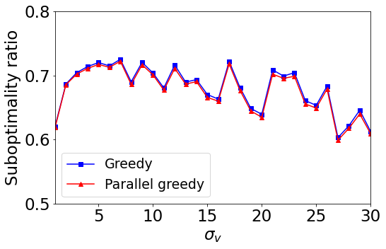
(a) a

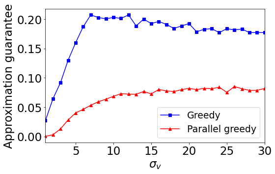
(b) b

Figure 1: Actual performances and approximation guarantees of Algorithms 1-2.

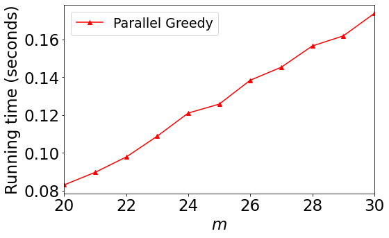
(a) a

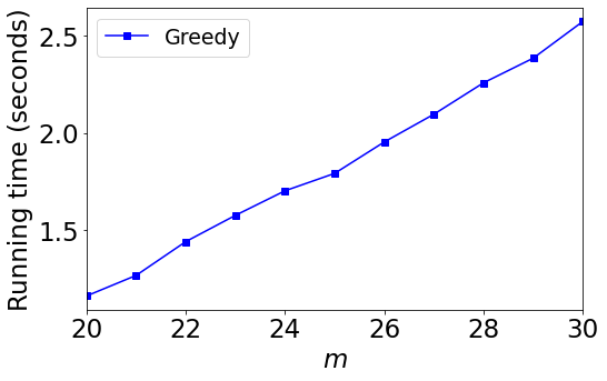
(b) b

Figure 2: Running times of Algorithms 1-2.

6 Conclusion

We studied the problem of maximizing a monotone nondecreasing set function under multiple constraints, where the constraints are upper bound constraints characterized by monotone nondecreasing set functions. We proposed two greedy algorithms to solve the problem, and analyzed the approximation guarantees of the algorithms, leveraging the notions of submodularity ratio and curvature of set functions. We discussed several important real-world applications of the general problem, and provided bounds on the submodularity ratio and curvature of the set functions in the corresponding instances of the problem. Numerical results show that the two greedy algorithms yield comparable performances that are reasonably good in practice.

Appendix A Proof of Theorem 6

Lemma 17.

Under the setting of Theorem 6, we have

$$f(\mathcal{A}_{i}^{r})\geq\frac{\min\{1,\tilde{\gamma}_{f}\}}{2}(1-e^{-(1-\tilde{\alpha}_{i})\gamma_{f}})f(\mathcal{A}_{i}^{\star}),$$ (20)

for all $i\in[n]$.

Under Assumption 4, we see from the definitions of (P1) and Algorithm 1 that $A^{r}=\cup_{i\in[n]}\mathcal{A}^{r}_{i}$ and $\mathcal{A}^{\star}=\cup_{i\in[n]}\mathcal{A}^{\star}_{i}$, where $\mathcal{A}_{i}^{r},\mathcal{A}_{i}^{\star}\subseteq\mathcal{S}_{i}$ for all $i\in[n]$, and $\mathcal{A}_{i}^{r}\cap\mathcal{A}_{j}^{r}=\emptyset$, $\mathcal{A}_{i}^{\star}\cap\mathcal{A}_{j}^{\star}=\emptyset$ for all $i,j\subseteq[n]$ with $i\neq j$. Now, considering any $i\in[n]$, we note that (20) trivially holds if $\tilde{\gamma}_{f}=0$, $\gamma_{f}=0$ or $\tilde{\alpha}_{i}=1$. Thus, in the remaining of this proof, we let $\tilde{\gamma}_{f}\in\mathbb{R}_{>0}$, $\gamma_{f}\in(0,1]$ and $\tilde{\alpha}_{i}\in[0,1)$. Recalling that we have assumed that $h_{i}(v)>0$ for all $v\in\mathcal{S}$, we then have from Definition 2 that $\delta_{v}^{i}(\mathcal{A})>0$ for all $\mathcal{A}\subseteq\mathcal{S}$ and for all $v\in\mathcal{S}\setminus\mathcal{A}$, which implies that line 5 of Algorithm 1 is well-defined. Recall from Observation 1 that $\mathcal{A}_{i,j}^{r}=\{q_{1},\dots,q_{j}\}$ for all $j\in[|\mathcal{A}_{i}^{r}|]$ with $\mathcal{A}_{i,0}^{r}=\emptyset$. Moreover, denote $\tilde{\mathcal{A}}_{i,j}=\{\tilde{q}_{1},\dots,\tilde{q}_{j}\}$ for all $j\in[l_{i}+1]$ with $\tilde{\mathcal{A}}_{i,0}=\emptyset$, where $\tilde{q}_{i}=q_{i}$ for all $i\in[l_{i}]$ and $\tilde{q}_{j+1}=v^{\star}_{l_{i}+1}$, where $l_{i}$ and $v_{l_{i}+1}^{\star}$ are given in Observation 1. Now, considering any $j\in\{0,1,\dots,l_{i}\}$ and denoting $\tilde{\mathcal{A}}^{\star}_{i}=\mathcal{A}_{i}^{\star}\setminus\tilde{\mathcal{A}}_{i,j}^{r}=\{p_{1},\dots,p_{|\tilde{\mathcal{A}}_{i}^{\star}|}\}$, we have

$$f(\mathcal{A}^{\star}_{i}\cup\tilde{\mathcal{A}}^{r}_{i,j})-f(\tilde{\mathcal{A}}^{r}_{i,j})\leq\frac{1}{\gamma_{f}}\sum_{k=1}^{|\tilde{A}^{\star}_{i}|}\delta_{p_{k}}(\tilde{\mathcal{A}}_{i,j}^{r})$$

$$= \frac{1}{\gamma_{f}}\sum_{k=1}^{|\tilde{A}^{\star}_{i}|}\frac{\delta_{p_{k}}(\tilde{\mathcal{A}}_{i,j})}{\delta^{i}_{p_{k}}(\tilde{\mathcal{A}}_{i,j}^{r})}\delta^{i}_{p_{k}}(\tilde{\mathcal{A}}_{i,j}^{r})\leq\frac{\delta_{\tilde{q}_{j+1}}(\tilde{\mathcal{A}}_{i,j}^{r})}{\gamma_{f}\delta^{i}_{\tilde{q}_{j+1}}(\tilde{\mathcal{A}}_{i,j}^{r})}\sum_{k=1}^{|\tilde{\mathcal{A}}^{\star}_{i}|}\delta^{i}_{p_{k}}(\tilde{\mathcal{A}}_{i,j}^{r})$$

$$\leq \frac{\delta_{\tilde{q}_{j+1}}(\tilde{A}_{i,j}^{r})}{\delta^{i}_{\tilde{q}_{j+1}}(\tilde{\mathcal{A}}_{i,j}^{r})\gamma_{f}(1-\tilde{\alpha}_{i})}\sum_{k=1}^{|\tilde{\mathcal{A}}^{\star}_{i}|}\delta^{i}_{p_{k}}(\{p_{1},\dots,p_{k-1}\})$$

$$= \frac{\delta_{\tilde{q}_{j+1}}(\tilde{\mathcal{A}}_{i,j}^{r})}{(h_{i}(\tilde{\mathcal{A}}_{i,j+1}^{r})-h_{i}(\tilde{\mathcal{A}}_{i,j}^{r}))\gamma_{f}(1-\tilde{\alpha}_{i})}h_{i}(\tilde{\mathcal{A}}_{i}^{\star}),$$ (21)

where the first inequality follows from Definition 1, the second inequality follows from the greedy choice in line 5 of Algorithm 1, and the third inequality follows from Definition 2. To proceed, denoting $\Delta_{j}\triangleq f(\mathcal{A}^{\star}_{i})-f(\tilde{\mathcal{A}}^{r}_{i,j})$ for all $j\in\{0,1,\dots,l_{i}+1\}$, and noting that $h_{i}(\tilde{\mathcal{A}}^{\star}_{i})\leq h_{i}(\mathcal{A}_{i}^{\star})\leq H_{i}$, we have from (21) the following:

$$\Delta_{j+1}\leq\big{(}1-\frac{\gamma_{f}(1-\tilde{\alpha}_{i})(h_{i}(\tilde{\mathcal{A}}_{i,j+1}^{r})-h_{i}(\tilde{\mathcal{A}}_{i,j}^{r}))}{H_{i}}\big{)}\Delta_{j}$$

$$\Rightarrow \Delta_{l_{i}+1}\leq\Delta_{0}\prod_{j=0}^{l_{i}}\big{(}1-\frac{\gamma_{f}(1-\tilde{\alpha}_{i})(h_{i}(\tilde{A}_{i,j+1}^{r})-h_{i}(\tilde{\mathcal{A}}_{i,j}^{r}))}{H_{i}}\big{)}$$

$$\qquad\leq\Delta_{0}\prod_{j=0}^{l_{i}}\big{(}1-\frac{\gamma_{f}(1-\tilde{\alpha}_{i})(h_{i}(\tilde{\mathcal{A}}_{i,j+1}^{r})-h_{i}(\tilde{\mathcal{A}}_{i,j}^{r}))}{h_{i}(\tilde{\mathcal{A}}_{i,l_{i}+1}^{r})}\big{)},$$

where the third inequality follows from $h_{i}(\tilde{\mathcal{A}}_{i,l_{i}+1}^{r})>H_{i}$ as we argued above. Note the fact that if $a_{1},\dots,a_{n}\in\mathbb{R}_{>0}$ such that $\sum_{i=1}^{n}a_{i}=\alpha G$, where $G\in\mathbb{R}_{>0}$ and $\alpha\in(0,1]$, then the function $\Pi_{i=1}^{n}(1-\frac{a_{i}}{G})$ achieves its maximum at $a_{1}=\cdots=a_{n}=\frac{\alpha G}{n}$ [24]. Since $\sum_{j=0}^{l_{i}}(h_{i}(\tilde{\mathcal{A}}_{i,j+1}^{r})-h_{i}(\tilde{\mathcal{A}}_{i,j}^{r}))=h_{i}(\tilde{\mathcal{A}}_{i,l_{i}+1}^{r})$ and $\gamma_{f}(1-\tilde{\alpha}_{i})<1$, we have

$$\prod_{j=0}^{l_{i}}\big{(}1-\frac{\gamma_{f}(1-\tilde{\alpha}_{i})(h_{i}(\tilde{\mathcal{A}}_{i,j+1}^{r})-h_{i}(\tilde{\mathcal{A}}_{i,j}^{r}))}{h_{i}(\tilde{A}_{i,l_{i}+1}^{r})}\big{)}$$

$$\leq \prod_{j=0}^{l_{i}}\big{(}1-\frac{\gamma_{f}(1-\tilde{\alpha}_{i})\frac{h_{i}(\tilde{\mathcal{A}}_{i,l_{i}+1}^{r})}{l_{i}+1}}{h_{i}(\tilde{\mathcal{A}}_{i,l_{i}+1}^{r})}\big{)}=\big{(}1-\frac{\gamma_{f}(1-\tilde{\alpha}_{i})}{l_{i}+1}\big{)}^{l_{i}+1}.$$

It follows that

$$\Delta_{l_{i}+1}\leq\big{(}1-\frac{\gamma_{f}(1-\tilde{\alpha}_{i})}{l_{i}+1}\big{)}^{l_{i}+1}\Delta_{0}\leq e^{-\gamma_{f}(1-\tilde{\alpha}_{i})}\Delta_{0}$$

$$\Rightarrow\ f(\tilde{\mathcal{A}}_{i,l_{i}+1}^{r})\geq(1-e^{-\gamma_{f}(1-\tilde{\alpha}_{i})})f(\mathcal{A}^{\star}_{i}).$$ (22)

Recalling from Definition 5 that $f(\tilde{\mathcal{A}}_{i,l_{i}+1}^{r})-f(\tilde{\mathcal{A}}_{i,l_{i}}^{r})\leq\frac{1}{\tilde{\gamma}_{f}}f(\mathcal{B}_{i}^{r})$, we obtain from (22) that $f(\tilde{\mathcal{A}}_{i,l_{i}}^{r})+\frac{1}{\tilde{\gamma}_{f}}f(\mathcal{B}_{i}^{r})\geq(1-e^{-\gamma_{f}(1-\tilde{\alpha}_{i})})f(\mathcal{A}_{i}^{\star})$. Since $f(\cdot)$ is monotone nondecreasing, it follows that $f(\mathcal{A}_{i}^{r})+\frac{1}{\tilde{\gamma}_{f}}f(\mathcal{B}_{i}^{r})\geq(1-e^{-\gamma_{f}(1-\tilde{\alpha}_{i})})f(\mathcal{A}_{i}^{\star})$, which implies that at least one of $f(\mathcal{A}_{i}^{r})$ and $\frac{1}{\tilde{\gamma}_{f}}f(\mathcal{B}_{i}^{r})$ is greater than or equal to $\frac{1}{2}(1-e^{-\gamma_{f}(1-\tilde{\alpha}_{i})})f(\mathcal{A}_{i}^{\star})$. Thus, we see from line 9 in Algorithm 1 that (20) holds. $\blacksquare$ Proof of Theorem 6: Since (6) naturally holds if $\kappa_{f}=0$, we let $\kappa_{f}\in(0,1]$ in this proof. Considering $\mathcal{A}^{r}=\cup_{i\in[n]}\mathcal{A}_{i}^{r}$ returned by Algorithm 1, and denoting $\mathcal{A}_{1}=\cup_{i\in[n-1]}\mathcal{A}_{i}^{r}$ and $\mathcal{A}_{2}=\mathcal{A}_{n}^{r}=\{q_{1},\dots,q_{|\mathcal{A}_{n}^{r}|}\}$, we have

$$f(\mathcal{A}_{1}\cup\mathcal{A}_{2}) =f(\mathcal{A}_{1})+\sum_{j=1}^{|\mathcal{A}_{n}^{r}|}\delta_{q_{j}}(\mathcal{A}_{1}\cup\{q_{1},\dots,q_{j-1}\})$$

$$\geq f(\mathcal{A}_{1})+(1-\alpha_{f})\sum_{j=1}^{|\mathcal{A}_{n}^{r}|}\delta_{q_{j}}(\{q_{1},\dots,q_{j-1}\})$$

$$=f(\mathcal{A}_{1})+(1-\alpha_{f})f(\mathcal{A}_{2}).$$ (23)

where the inequality uses the fact that $q_{j}\notin A_{1}$ (from Assumption 4) and Definition 2. Repeating the above arguments for (23), one can show that $f(\cup_{i\in[n]}\mathcal{A}_{i}^{r})\geq(1-\alpha_{f})\sum_{i=1}^{n}f(\mathcal{A}_{i}^{r})$, which implies via (20) that

$$f(\mathcal{A}^{r})\geq\frac{(1-\alpha_{f})\min\{1,\tilde{\gamma}_{f}\}}{2}\\ \times\min_{i\in[n]}(1-e^{-(1-\tilde{\alpha}_{i})\gamma_{i}})\sum_{i=1}^{n}f(\mathcal{A}_{i}^{\star}).$$ (24)

Now, consider the optimal solution $\mathcal{A}^{\star}=\cup_{i\in[n]}\mathcal{A}_{i}^{\star}$. Using similar arguments to those above, and recalling the definition of the DR ratio $\kappa_{f}$ of $f(\cdot)$ given in Definition 1, one can show that $f(\cup_{i\in[n]}\mathcal{A}_{i}^{\star})\leq\frac{1}{\kappa_{f}}\sum_{i=1}^{n}f(\mathcal{A}_{i}^{\star})$, which together with (24) complete the proof of (6). $\blacksquare$

Appendix B Proof of Theorem 9

First, note that (8) trivially holds if $\gamma_{f}=0$, $\alpha_{h}=1$, or $f(\mathcal{A}^{\star})=0$. Thus, we let $\gamma_{f}\in(0,1]$, $\tilde{\alpha}_{i}\in[0,1)$, and $f(\mathcal{A}^{\star})>0$ in this proof. For our analysis in this proof, we assume without loss of generality that $f(\cdot)$ is normalized such that $f(\mathcal{A}^{\star})=1$. Also recalling that we have assumed that $h_{i}(v)>0$ for all $v\in\mathcal{S}$, we know from Definition 2 that $\delta^{i}_{v}(\mathcal{A})=h_{i}(\mathcal{A}\cup\{v\})-h_{i}(\mathcal{A})>0$ for all $\mathcal{A}\subseteq\mathcal{S}$ and for all $v\in\mathcal{S}\setminus\mathcal{A}$, which implies that $\psi_{j}$ in Definition 8 and line 3 of Algorithm 1 are well-defined. Denote $\mathcal{A}^{g}=\{q_{1},\dots,q_{|\mathcal{A}^{g}|}\}$, and $\mathcal{A}^{g}_{j}=\{q_{1},\dots,q_{j}\}$ for all $j\in[|\mathcal{A}^{g}|]$ with $\mathcal{A}^{g}_{0}=\emptyset$. We claim that in the remaining of this proof, we can further assume without loss of generality that $\psi_{j}>0$ for all $j\in\{0,\dots,|\mathcal{A}^{g}|-1\}$. To prove this claim, we first assume (for contradiction) that there exists $j\in\{0,\dots,|\mathcal{A}^{g}|-1\}$ such that $\delta_{q_{j+1}}(\mathcal{A}^{g}_{j})=0$. Since $\gamma_{f}\in(0,1]$ as we argued above, we see from Definition 1 and the greedy choice that $\delta_{\mathcal{W}}(\mathcal{A}^{g}_{j})=0$, where $\mathcal{W}$ is defined and iteratively updated in Algorithm 2. Recalling that $f(\cdot)$ is monotone nondecreasing as we assumed before, we then have that $f(\mathcal{A}^{g}_{j}\cup\mathcal{W}_{1})=f(\mathcal{A}^{g}_{j}\cup\mathcal{W}_{2})$ for all $\mathcal{W}_{1},\mathcal{W}_{2}\subseteq\mathcal{W}$. It follows that $\delta_{q_{j^{\prime}+1}}(\mathcal{A}^{g}_{j^{\prime}})=0$ for all $j^{\prime}\in\{j,\dots,|\mathcal{A}^{g}|-1\}$. In other words, Algorithm 2 is vacuous after adding $q_{j}$ to the greedy solution $A^{g}$. Thus, we can assume without loss of generality that $\delta_{q_{j+1}}(\mathcal{A}_{j}^{g})>0$ for all $j\in\{0,\dots,|\mathcal{A}^{g}|-1\}$, which implies via Definition 8 that $\psi_{j}>0$ for all $j\in\{0,\dots,|\mathcal{A}^{g}|-1\}$.

To proceed, let us consider any $j\in\{0,\dots,|\mathcal{A}^{g}|-1\}$. Denoting $\tilde{\mathcal{A}}_{j}^{\star}=\mathcal{A}^{\star}\setminus\mathcal{A}_{j}^{g}$, we have

$$f(\mathcal{A}^{\star}) \leq f(\mathcal{A}_{j}^{g})+\frac{1}{\gamma_{f}}\sum_{v\in\tilde{\mathcal{A}}^{\star}_{j}}\delta_{v}(A^{g}_{j})$$

$$\leq f(\mathcal{A}_{j}^{g}) +\frac{1}{\gamma_{f}}\sum_{i\in[n]}\sum_{v\in\tilde{A}^{\star}_{j}\cap\mathcal{S}_{i}}\frac{\delta_{v}(\mathcal{A}_{j}^{g})}{\delta_{v}^{i}(\mathcal{A}^{g}_{j})}\delta_{v}^{i}(\mathcal{A}_{j}^{g})$$

$$\leq f(\mathcal{A}_{j}^{g}) +\frac{\delta_{q_{j+1}}(\mathcal{A}_{j}^{g})}{\gamma_{f}\psi_{j}\delta^{i_{j}}_{q_{j+1}}(\mathcal{A}_{j}^{g})}\sum_{i\in[n]}\sum_{v\in\tilde{\mathcal{A}}^{\star}_{j}\cap\mathcal{S}_{i}}\delta^{i}_{v}(\mathcal{A}_{j}^{g}),$$ (25)

where the first inequality follows from Definition 1 and the monotonicity of $f(\cdot)$, and the third inequality follows from Definition 8. Denoting $\tilde{\mathcal{A}}^{\star}_{j}\cap\mathcal{S}_{i}=\{p^{i}_{1},\dots,p^{i}_{|\tilde{\mathcal{A}}^{\star}_{j}\cap\mathcal{S}_{i}|}\}$ for all $i\in[n]$, we further obtain from Definition 2 that

$$\sum_{i\in[n]}\sum_{v\in\tilde{\mathcal{A}}^{\star}_{j}\cap\mathcal{S}_{i}}\delta^{i}_{v}(\mathcal{A}_{j}^{g})$$

$$\leq \frac{1}{1-\alpha_{h}}\sum_{i\in[n]}\sum_{k=1}^{|\tilde{\mathcal{A}}^{\star}_{j}\cap S_{i}|}\delta^{i}_{p^{i}_{k}}(\{p_{1}^{i},\dots,p_{k-1}^{i}\})$$

$$= \frac{1}{1-\alpha_{h}}\sum_{i\in[n]}h_{i}(\tilde{\mathcal{A}}^{\star}_{j}\cap\mathcal{S}_{i})\leq\frac{\sum_{i\in[n]}H_{i}}{1-\alpha_{h}}.$$ (26)

Denoting

$$M_{j}=\frac{\sum_{i\in[n]}H_{i}}{(1-\alpha_{h})\gamma_{f}\psi_{j}\delta^{i_{j}}_{q_{j+1}}(\mathcal{A}_{j}^{g})},$$ (27)

and $\delta_{j}=\delta_{q_{j+1}}(\mathcal{A}_{j}^{g})$ for all $j\in\{0,\dots,|\mathcal{A}^{g}|-1\}$, we can combine (25)-(26) and obtain that

$$M_{j}\delta_{j}+\sum_{k=0}^{j-1}\delta_{k}\geq 1,\ \forall j\in\{0,\dots,|\mathcal{A}^{g}|-1\},$$ (28)

where we use the facts that $f(\mathcal{A}^{g}_{j})=\sum_{k=0}^{j-1}\delta_{k}$ and $f(\mathcal{A}^{\star})=1$ as we argued before.

In order to prove the approximation guarantee of Algorithm 2 given by (8), we aim to provide a lower bound on $f(\mathcal{A}^{g})/f(\mathcal{A}^{\star})$ and we achieve this by first minimizing $f(\mathcal{A}^{g})/f(\mathcal{A}^{\star})=\sum_{j=0}^{|\mathcal{A}^{g}|-1}\delta_{j}$ subject to the constraints given in (28). In other words, we consider the following linear program and its dual:

$$\begin{split}&\min_{\delta_{j}}\sum_{j=0}^{|\mathcal{A}^{g}|-1}\delta_{j}\\ &s.t.\ M_{j}\delta_{j}+\sum_{k=0}^{j-1}\delta_{k}\geq 1,\ \forall j\in\{0,\dots,|\mathcal{A}^{g}|-1\},\end{split}$$ (29)

$$\begin{split}&\max_{\mu_{k}}\sum_{k=0}^{|\mathcal{A}^{g}|-1}\mu_{k}\\ &s.t.\ \mu_{k}\geq 0,\ \forall k\in\{0,\dots,|\mathcal{A}^{g}|-1\}\\ &\ \ \ M_{j}\mu_{j}+\sum_{k=j+1}^{|A^{g}|-1}\mu_{k}=1,\ \forall j\in\{0,\dots,|\mathcal{A}^{g}|-1\}.\end{split}$$ (30)

We will then show that the optimal cost of (29) and (30) satisfies (8). Noting from Eq. (27) that $M_{j}>0$ for all $j\in\{0,\dots,|\mathcal{A}^{g}|-1\}$, we can obtain the optimal solution to (30) by solving the equations in $u_{k}$ given by the equality constraints in (30), which yields $\mu_{k}^{\star}=\frac{1}{M_{k}}\prod_{j=k+1}^{|\mathcal{A}^{g}|-1}(1-\frac{1}{M_{j}})$ $\forall k\in\{0,\dots,|\mathcal{A}^{g}|-1\}$. Noting from Eq. (27) that $\sum_{k=0}^{|\mathcal{A}^{g}|-1}\frac{1}{M_{k}}=B$, we can further lower bound $\sum_{k=0}^{|\mathcal{A}^{g}|-1}\mu_{k}^{\star}$ by solving

$$\begin{split}\min_{\nu_{k}}\sum_{k=0}^{|A^{g}|-1}\nu_{k}\prod_{j=k+1}^{|\mathcal{A}^{g}|-1}(1-\nu_{j})\quad s.t.\ \sum_{k=0}^{|\mathcal{A}^{g}|-1}\nu_{k}=B.\end{split}$$ (31)

One can obtain the optimal solution to (31) by considering a Lagrangian multiplier corresponding to the equality constraint in (31), which yields the optimal solution $\nu_{k}=\frac{B}{|\mathcal{A}^{g}|}$ $\forall k\in\{0,\dots,|\mathcal{A}^{g}|-1\}$. It then follows from our arguments above that

$$\sum_{k=0}^{|\mathcal{A}^{g}|-1}\mu_{k}^{\star} \geq\sum_{k=0}^{|\mathcal{A}^{g}|-1}\frac{B}{|\mathcal{A}^{g}|}\prod_{j=k+1}^{|\mathcal{A}^{g}|-1}(1-\frac{B}{|\mathcal{A}^{g}|})$$

$$=1-(1-\frac{B}{|\mathcal{A}^{g}|})^{|\mathcal{A}^{g}|}\geq 1-e^{-B}.\qquad\qquad\quad\hfill\blacksquare$$

References

• [1] Brian DO Anderson and John B Moore. Optimal Filtering. Dover Books, 1979.
• [2] Ravikumar Balakrishnan, Tian Li, Tianyi Zhou, Nageen Himayat, Virginia Smith, and Jeff Bilmes. Diverse client selection for federated learning via submodular maximization. In Proc. International Conference on Learning Representations, 2021.
• [3] Andrew An Bian, Joachim M Buhmann, Andreas Krause, and Sebastian Tschiatschek. Guarantees for greedy maximization of non-submodular functions with applications. In Proc. International Conference on Machine Learning, pages 498–507, 2017.
• [4] Gruia Calinescu, Chandra Chekuri, Martin Pal, and Jan Vondrák. Maximizing a monotone submodular function subject to a matroid constraint. SIAM Journal on Computing, 40(6):1740–1766, 2011.
• [5] Luiz FO Chamon, George J Pappas, and Alejandro Ribeiro. The mean square error in Kalman filtering sensor selection is approximately supermodular. In Proc. IEEE Conference on Decision and Control, pages 343–350, 2017.
• [6] Sundeep Prabhakar Chepuri and Geert Leus. Sparsity-promoting sensor selection for non-linear measurement models. IEEE Transactions on Signal Processing, 63(3):684–698, 2014.
• [7] Michele Conforti and Gérard Cornuéjols. Submodular set functions, matroids and the greedy algorithm: tight worst-case bounds and some generalizations of the rado-edmonds theorem. Discrete Applied Mathematics, 7(3):251–274, 1984.
• [8] Abhimanyu Das and David Kempe. Submodular meets spectral: Greedy algorithms for subset selection, sparse approximation and dictionary selection. In Proc. International Conference on Machine Learning, pages 1057–1064, 2011.
• [9] Abhimanyu Das and David Kempe. Approximate submodularity and its applications: Subset selection, sparse approximation and dictionary selection. Journal of Machine Learning Research, 19(1):74–107, 2018.
• [10] Canh T Dinh, Nguyen H Tran, Minh NH Nguyen, Choong Seon Hong, Wei Bao, Albert Y Zomaya, and Vincent Gramoli. Federated learning over wireless networks: Convergence analysis and resource allocation. IEEE/ACM Transactions on Networking, 29(1):398–409, 2020.
• [11] S Durga, Rishabh Iyer, Ganesh Ramakrishnan, and Abir De. Training data subset selection for regression with controlled generalization error. In Proc. International Conference on Machine Learning, pages 9202–9212, 2021.
• [12] Ethan R Elenberg, Rajiv Khanna, Alexandros G Dimakis, and Sahand Negahban. Restricted strong convexity implies weak submodularity. The Annals of Statistics, 46(6B):3539–3568, 2018.
• [13] Uriel Feige. A threshold of $\ln n$ for approximating set cover. Journal of the ACM (JACM), 45(4):634–652, 1998.
• [14] Marshall L Fisher, George L Nemhauser, and Laurence A Wolsey. An analysis of approximations for maximizing submodular set functions—ii. In Polyhedral Combinatorics, pages 73–87. Springer, 1978.
• [15] Vijay Gupta, Timothy H Chung, Babak Hassibi, and Richard M Murray. On a stochastic sensor selection algorithm with applications in sensor scheduling and sensor coverage. Automatica, 42(2):251–260, 2006.
• [16] Marco F Huber. Optimal pruning for multi-step sensor scheduling. IEEE Transactions on Automatic Control, 57(5):1338–1343, 2011.
• [17] Rishabh Iyer and Jeff Bilmes. Algorithms for approximate minimization of the difference between submodular functions, with applications. In Proc. Conference on Uncertainty in Artificial Intelligence, pages 407–417, 2012.
• [18] Syed Talha Jawaid and Stephen L Smith. Submodularity and greedy algorithms in sensor scheduling for linear dynamical systems. Automatica, 61:282–288, 2015.
• [19] Siddharth Joshi and Stephen Boyd. Sensor selection via convex optimization. IEEE Transactions on Signal Processing, 57(2):451–462, 2008.
• [20] Samir Khuller, Anna Moss, and Joseph Seffi Naor. The budgeted maximum coverage problem. Information Processing Letters, 70(1):39–45, 1999.
• [21] Akira Kohara, Kunihisa Okano, Kentaro Hirata, and Yukinori Nakamura. Sensor placement minimizing the state estimation mean square error: Performance guarantees of greedy solutions. In Proc. IEEE Conference on Decision and Control, pages 1706–1711, 2020.
• [22] Andreas Krause, Ajit Singh, and Carlos Guestrin. Near-optimal sensor placements in Gaussian processes: Theory, efficient algorithms and empirical studies. Journal of Machine Learning Research, 9(Feb):235–284, 2008.
• [23] Alan Kuhnle, J David Smith, Victoria Crawford, and My Thai. Fast maximization of non-submodular, monotonic functions on the integer lattice. In Proc. International Conference on Machine Learning, pages 2786–2795, 2018.
• [24] Ariel Kulik, Hadas Shachnai, and Tami Tamir. Maximizing submodular set functions subject to multiple linear constraints. In Proc. annual ACM-SIAM Symposium on Discrete Algorithms, pages 545–554, 2009.
• [25] Jure Leskovec, Andreas Krause, Carlos Guestrin, Christos Faloutsos, Jeanne VanBriesen, and Natalie Glance. Cost-effective outbreak detection in networks. In Proc. International Conference on Knowledge Discovery and Data Mining, pages 420–429, 2007.
• [26] Xiang Li, Kaixuan Huang, Wenhao Yang, Shusen Wang, and Zhihua Zhang. On the convergence of FedAvg on non-iid data. In Proc. International Conference on Learning Representations, 2020.
• [27] Brendan McMahan, Eider Moore, Daniel Ramage, Seth Hampson, and Blaise Aguera y Arcas. Communication-efficient learning of deep networks from decentralized data. In Proc. Artificial Intelligence and Statistics, pages 1273–1282, 2017.
• [28] Yilin Mo, Roberto Ambrosino, and Bruno Sinopoli. Sensor selection strategies for state estimation in energy constrained wireless sensor networks. Automatica, 47(7):1330–1338, 2011.
• [29] George L Nemhauser, Laurence A Wolsey, and Marshall L Fisher. An analysis of approximations for maximizing submodular set functions—i. Mathematical Programming, 14(1):265–294, 1978.
• [30] Takayuki Nishio and Ryo Yonetani. Client selection for federated learning with heterogeneous resources in mobile edge. In Proc. IEEE International Conference on Communications, pages 1–7, 2019.
• [31] Amritha Prasad, Jeffrey Hudack, Shaoshuai Mou, and Shreyas Sundaram. Policies for risk-aware sensor data collection by mobile agents. Automatica, 142:110391, 2022.
• [32] Amirhossein Reisizadeh, Aryan Mokhtari, Hamed Hassani, Ali Jadbabaie, and Ramtin Pedarsani. Fedpaq: A communication-efficient federated learning method with periodic averaging and quantization. In Proc. International Conference on Artificial Intelligence and Statistics, pages 2021–2031, 2020.
• [33] Wenqi Shi, Sheng Zhou, Zhisheng Niu, Miao Jiang, and Lu Geng. Joint device scheduling and resource allocation for latency constrained wireless federated learning. IEEE Transactions on Wireless Communications, 20(1):453–467, 2020.
• [34] Vasileios Tzoumas, Luca Carlone, George J Pappas, and Ali Jadbabaie. LQG control and sensing co-design. IEEE Transactions on Automatic Control, 66(4):1468–1483, 2020.
• [35] Vasileios Tzoumas, Ali Jadbabaie, and George J Pappas. Sensor placement for optimal Kalman filtering: Fundamental limits, submodularity, and algorithms. In Proc. American Control Conference, pages 191–196, 2016.
• [36] Lintao Ye and Vijay Gupta. Client scheduling for federated learning over wireless networks: A submodular optimization approach. In Proc. IEEE Conference on Decision and Control, pages 63–68, 2021.
• [37] Lintao Ye, Philip E Paré, and Shreyas Sundaram. Parameter estimation in epidemic spread networks using limited measurements. SIAM Journal on Control and Optimization, 60(2):S49–S74, 2021.
• [38] Lintao Ye and Shreyas Sundaram. Sensor selection for hypothesis testing: Complexity and greedy algorithms. In Proc. IEEE Conference on Decision and Control, pages 7844–7849, 2019.
• [39] Lintao Ye, Nathaniel Woodford, Sandip Roy, and Shreyas Sundaram. On the complexity and approximability of optimal sensor selection and attack for Kalman filtering. IEEE Transactions on Automatic Control, 66(5):2146–2161, 2021.
• [40] Haotian Zhang, Raid Ayoub, and Shreyas Sundaram. Sensor selection for Kalman filtering of linear dynamical systems: Complexity, limitations and greedy algorithms. Automatica, 78:202–210, 2017.