Electron correlation effects on the $g$ factor of lithiumlike ions

Abstract

We present the systematic QED treatment of the electron correlation effects on the $g$ factor of lithiumlike ions for the wide range of nuclear charge number $Z=14$ – $82$. The one- and two-photon exchange corrections are evaluated rigorously within the QED formalism. The electron-correlation contributions of the third and higher orders are accounted for within the Breit approximation employing the recursive perturbation theory. The calculations are performed in the framework of the extended Furry picture, i.e., with inclusion of the effective local screening potential in the zeroth-order approximation. In comparison to the previous theoretical calculations, the accuracy of the interelectronic-interaction contributions to the bound electron $g$ factor in lithiumlike ions is substantially improved.

I Introduction

Over the past decades, the bound-electron $g$ factor remains a subject of intense theoretical and experimental studies. Nowadays, the $g$ factor of H-like ions is measured with a relative accuracy of up to few parts in $10^{11}$ Häffner et al. (2000); Verdú et al. (2004); Sturm et al. (2011, 2013, 2014); Sailer et al. (2022). These measurements combined with the theoretical studies Persson et al. (1997); Blundell et al. (1997); Beier (2000); Karshenboim (2000); Karshenboim et al. ; Glazov and Shabaev (2002); Shabaev and Yerokhin (2002); Nefiodov et al. (2002); Yerokhin et al. (2002); Pachucki et al. (2005); Jentschura (2009); Yerokhin and Harman (2013); Yerokhin et al. (2013) have led to the most accurate up-to-date value of the electron mass Sturm et al. (2014). Present experimental techniques also allow for the $g$-factor measurements in few-electron ions Wagner et al. (2013); D. von Lindenfels, M. Wiesel, D. A. Glazov, A. V. Volotka, M. M. Sokolov, V. M. Shabaev, G. Plunien, W. Quint, G. Birkl, A. Martin, and M. Vogel (2013); F. Köhler, K. Blaum, M. Block, S. Chenmarev, S. Eliseev, D. A. Glazov, M. Goncharov, J. Hou, A. Kracke, D. A. Nesterenko, Yu. N. Novikov, W. Quint, E. Minaya Ramirez, V. M. Shabaev, S. Sturm, A. V. Volotka, and G. Werth (2016); Glazov et al. (2019); Arapoglou et al. (2019); Egl et al. (2019); Micke et al. (2020) with the accuracy comparable to that for H-like ions.

High-precision measurements of the $g$ factor of highly charged ions provide various opportunities to probe the non-trivial QED effects in strong electromagnetic fields, determine fundamental constants and nuclear properties, and strengthen the limits on the hypothetical physics beyond the Standard Model Yerokhin et al. (2011); Volotka et al. (2013); Shabaev et al. (2015); Indelicato (2019); Debierre et al. (2020); Shabaev et al. (2022); Debierre et al. (2022). For example, the measurement of the $g$-factor isotope shift with lithiumlike calcium ions F. Köhler, K. Blaum, M. Block, S. Chenmarev, S. Eliseev, D. A. Glazov, M. Goncharov, J. Hou, A. Kracke, D. A. Nesterenko, Yu. N. Novikov, W. Quint, E. Minaya Ramirez, V. M. Shabaev, S. Sturm, A. V. Volotka, and G. Werth (2016) has opened a possibility to test the relativistic nuclear recoil theory in the presence of magnetic field and paved the way to probe bound-state QED effects beyond the Furry picture in the strong-field regime Shabaev et al. (2017); Malyshev et al. (2017); Shabaev et al. (2018). The high-precision bound-electron $g$-factor experiments combined with theoretical studies are expected to provide an independent determination of the fine structure constant $\alpha$ Shabaev et al. (2006); Yerokhin et al. (2016a). While the $g$-factor calculations are progressing further Czarnecki and Szafron (2016); Yerokhin and Harman (2017); Czarnecki et al. (2018); Sikora et al. (2020); Oreshkina et al. (2020); Czarnecki et al. (2020); Debierre et al. (2021), the accuracy of theoretical values is ultimately limited by the finite-nuclear-size effect. To overcome this problem, it was proposed to use the so-called specific difference of the $g$ factors for two charge states of one isotope Shabaev et al. (2002, 2006); Volotka and Plunien (2014); Yerokhin et al. (2016a, b); Malyshev et al. (2017). It was demonstrated that the theoretical uncertainty of the specific difference can be made several orders of magnitude smaller than that of the individual $g$-factor values. Therefore, it is very important to consider not only hydrogenlike but also lithiumlike and boronlike ions.

The first experiments with lithiumlike ions were carried out for silicon Wagner et al. (2013) and calcium F. Köhler, K. Blaum, M. Block, S. Chenmarev, S. Eliseev, D. A. Glazov, M. Goncharov, J. Hou, A. Kracke, D. A. Nesterenko, Yu. N. Novikov, W. Quint, E. Minaya Ramirez, V. M. Shabaev, S. Sturm, A. V. Volotka, and G. Werth (2016) with an uncertainty of $10^{-9}$. Recently, the experimental value of the bound-electron $g$ factor in ²⁸Si¹¹⁺ was improved by a factor of 15 Glazov et al. (2019), and this is currently the most accurate value for few-electron ions. The theoretical value presented in Ref. Glazov et al. (2019) was 2 times more accurate than the previous one Volotka et al. (2014); Yerokhin et al. (2017), while the deviation from the experiment was $1.7\sigma$. Later, Yerokhin et al. undertook an independent evaluation of screened QED diagrams and obtained a new theoretical value for silicon Yerokhin et al. (2020) with smaller uncertainty and shifted farther from the experiment: $5.2\sigma$ deviation as a result. Then an independent evaluation of the two-photon-exchange diagrams was carried out to provide yet new results for lithiumlike silicon (with $3.1\sigma$ deviation) and calcium (with $4.2\sigma$ deviation) Yerokhin et al. (2021). Recently, we have thoroughly investigated the behaviour of many-electron QED contributions with various effective screening potentials Kosheleva et al. (2022), thus confirmed the results of Ref. Glazov et al. (2019) and reassured the agreement between theory and experiment.

In the present work, we provide detailed investigation of the electronic structure contributions and extend our calculations to a wide range of the nuclear charge number $Z$. The leading-order interelectronic-interaction terms corresponding to the one- and two-photon-exchange diagrams nowadays are calculated rigorously, i.e., to all orders in $\alpha Z$ Volotka et al. (2012); Wagner et al. (2013); Volotka et al. (2014); Yerokhin et al. (2021); Kosheleva et al. (2022). The contributions of the third and higher orders are taken into account approximately, to the leading orders in $\alpha Z$. This can be accomplished within different methods, which can yield slightly different results due to the incomplete treatment of the higher orders in $\alpha Z$. We use the Dirac-Coulomb-Breit (DCB) Hamiltonian and include the contribution of the negative-energy states Glazov et al. (2004). In Refs. Glazov et al. (2004, 2005); Volotka et al. (2014) the DCB equation was solved within the configuration interaction method Bratzev et al. (1977). Later, in Refs. Glazov et al. (2019); Kosheleva et al. (2022) the recursive perturbation theory was applied and proved to yield better accuracy. Moreover, we use the extended Furry picture, i.e., an effective local screening potential is included in the zeroth-order approximation along with the nuclear potential. The extended Furry picture provides partial account for the interelectronic interaction already in the zeroth order. As a result, there is a significant reduction of the perturbation theory terms in comparison to the case of the Coulomb potential. In particular, this leads to smaller uncertainty due to unknown non-trivial QED part of the third and higher-order contributions. The calculations are carried out with different screening potentials, namely, core-Hartree (CH), Kohn-Sham (KS), Dirac-Hartree (DH), and Dirac-Slater (DS), with and without the Latter correction. We show that the influence of this correction on the final result is insignificant, while the accuracy of calculations without it is better by an order of magnitude. In the QED calculations of the first and second orders, two different gauges of the photon propagator, Coulomb and Feynman, are considered and the gauge invariance is demonstrated, which serves as an additional test of the correctness of our calculations. As a result, we substantially improve the accuracy of the electronic-structure contribution to the $g$ factor of lithiumlike ions through a wide range of the nuclear charge number $Z=14$ – $82$.

The paper is organized as follows. In Sec. II, the basic formulas for the bound-electron $g$ factor in few-electron ions are given. In Sec. III, we present the rigorous theoretical description of the interelectronic-interaction corrections of the first (III A), second (III B), and higher orders (III C). Finally, in Sec. IV, we report the obtained numerical results.

Relativistic units ($\hbar=1$, $c=1$, $m_{e}=1$) and the Heaviside charge unit [$\alpha=e^{2}/(4\pi)$, $e<0$] are used throughout the paper.

II Basic formulas

The interaction of the bound electron with the external magnetic field $\bm{B}$ is represented by the operator,

$$V_{\rm m}=-e\bm{\alpha}\cdot\bm{A(r)}=-\frac{e}{2}BU\,,$$ (1)

where, without loss of generality, $B$ is assumed to be aligned in $z$-direction, $U=[{\bf r}\times\bm{\alpha}]_{z}$ and $\bm{\alpha}$ is the Dirac-matrix vector. Weak magnetic field induces the linear energy level shift,

$$\Delta E=-\dfrac{e}{2}gm_{j}B\,,$$ (2)

where $g$ is the electronic $g$ factor and $m_{j}$ is the $z$-projection of the total angular momentum $j$. In the case of one electron over the closed shells and a spinless nucleus, $m_{j}$ is determined by the valence electron state $|a\rangle=|j_{a}m_{a}\rangle$, with the angular momentum $j_{a}$ and its projection $m_{a}$. In the ground $(1s)^{2}\,2s$ state of a lithiumlike atom, this is just the $2s$ state.

The one-electron wave function obeys the Dirac equation,

$$h^{\rm D}|a\rangle=\varepsilon_{a}|a\rangle\,,\qquad h^{\rm D}=-i\bm{\alpha}\cdot\bm{\nabla}+\beta+V(r)\,,$$ (3)

where the binding potential $V(r)$ includes the nuclear potential and optionally some effective screening potential. Within the independent-electron approximation, the energy shift $\Delta E$ is found as an expectation value of $V_{\rm m}$ with $|a\rangle$, which yields the following expression for the $g$ factor,

$$g^{(0)}=\dfrac{1}{m_{a}}\langle a|U|a\rangle\,.$$ (4)

For the pure Coulomb nuclear potential, we denote the $g$ factor as $g^{(0)}_{\mathrm{C}}$. In the case of the point nucleus, $g^{(0)}_{\mathrm{C}}$ is known analytically (we denote it as $g_{\rm D}$) and for the $2s$ state given by the Breit formula Breit (1928):

$$g_{\rm D}=\dfrac{2}{3}(1+\sqrt{2+2\gamma})=2-\dfrac{(\alpha Z)^{2}}{6}+\dots\,,$$ (5)

where $\gamma=\sqrt{1-(\alpha Z)^{2}}$.

The total $g$-factor value comprises $g_{\rm D}$ and various corrections,

$$g=g_{\rm D}+\Delta g_{\rm int}+\Delta g_{\rm QED}+\Delta g_{\rm nuc}\,.$$ (6)

Here, $\Delta g_{\rm int}$ is the interelectronic-interaction correction which is the main topic of this work, $\Delta g_{\rm QED}$ is the QED correction previously investigated for lithiumlike ions, e.g., in Refs. Yerokhin et al. (2002, 2004); Glazov et al. (2006); Volotka et al. (2009); Glazov et al. (2010); Andreev et al. (2012); Volotka et al. (2014); Yerokhin and Harman (2017); Cakir et al. (2020); Yerokhin et al. (2020); Kosheleva et al. (2022), $\Delta g_{\rm nuc}$ stands for the nuclear size Karshenboim (2000); Glazov and Shabaev (2002); Yerokhin et al. (2013), nuclear recoil Shabaev and Yerokhin (2002); F. Köhler, K. Blaum, M. Block, S. Chenmarev, S. Eliseev, D. A. Glazov, M. Goncharov, J. Hou, A. Kracke, D. A. Nesterenko, Yu. N. Novikov, W. Quint, E. Minaya Ramirez, V. M. Shabaev, S. Sturm, A. V. Volotka, and G. Werth (2016); Shabaev et al. (2017); Malyshev et al. (2017); Shabaev et al. (2018) and nuclear polarization Nefiodov et al. (2002); Volotka and Plunien (2014) effects.

In the present work we focus on the electronic-structure contribution $\Delta g_{\rm int}$ to the ground-state $g$ factor of lithiumlike ions. The evaluation procedure for $\Delta g_{\rm int}$ is described in the following section. Here, we discuss an important aspect of this procedure — the choice of the zeroth-order approximation, which is defined by the potential $V(r)$ in the Dirac equation (3). In the original Furry picture it is the Coulomb potential $V_{\rm C}(r)$ generated by the nucleus. So, the interelectronic interaction is completely neglected at this stage. In present work we consider the extended Furry picture, which is based on the Dirac equation in the presence of an effective potential $V_{\rm eff}(r)$,

$$V_{\rm eff}(r)=V_{\rm C}(r)+V_{\rm scr}(r)\,,$$ (7)

where $V_{\rm scr}(r)$ is some local screening potential. This approach accelerates the convergence of perturbation theory, at least within the several leading orders, by accounting for a part of the interelectronic interaction already in the zeroth order. Another advantage of the screening potential is that it lifts the near-degeneracy of the $(1s)^{2}2s$ and $(1s)^{2}2p_{1/2}$ states occurring for the Coulomb potential. This helps to avoid the problems with additional singularities arising from the corresponding intermediate states, which are especially nuisance in the QED calculations involving energy integration. In particular, a subtraction procedure was used in Ref. Yerokhin et al. (2021) in order to deal with these singularities for the Coulomb potential.

Following our previous investigations, we employ 5 binding potentials: Coulomb, core-Hartree, Dirac-Hartree, Kohn-Sham, and Dirac-Slater. A well-known choice of $V_{\rm eff}({\bf r})$ is the core-Hartree (CH) potential

$$V_{\rm eff}(r)=V_{\rm C}(r)+\alpha\int^{\infty}_{0}dr^{\prime}\dfrac{1}{r_{>}}\rho_{c}(r^{\prime}).$$ (8)

Here $\rho_{c}$ is the density of the core (closed shells) electrons,

$$\rho_{c}(r^{\prime})=\sum_{\kappa_{c},n_{c}}(2j_{c}+1)(G^{2}_{c}(r)+F^{2}_{c}(r)),$$ (9)

where $\kappa_{c}$ and $n_{c}$ are the quantum numbers of the closed shells, $G_{c}$ and $F_{c}$ are the corresponding radial components of the wave function. The potential derived from the density functional theory reads

$$V_{\rm eff}(r)=V_{\rm C}(r)+\alpha\int^{\infty}_{0}dr^{\prime}\dfrac{1}{r_{>}}\rho_{t}(r^{\prime})-x_{\alpha}\dfrac{\alpha}{r}\left(\dfrac{81}{32\pi^{2}}r\rho_{t}(r)\right)^{1/3}.$$ (10)

Here $\rho_{t}$ is the total electron density, including the closed shells and the valence electron,

$$\rho_{t}(r)=(G^{2}_{a}(r)+F^{2}_{a}(r))+\sum_{\kappa_{c},n_{c}}(2j_{c}+1)(G^{2}_{c}(r)+F^{2}_{c}(r)).$$ (11)

The parameter $x_{\alpha}$ varies from $0$ to $1$. The cases of values $x_{\alpha}=0,\,2/3$, and $1$ are referred to as the Dirac-Hartree (DH), Kohn-Sham (KS), and Dirac-Slater (DS) potentials, respectively.

The DFT potentials as given by Eq. (10) possess non-physical asymptotic behavior. The Latter correction Latter (1955) circumvents this problem, but as a consequence the potentials cease to be smooth. The smoothing procedure itself can be different and therefore the potentials are barely reproducible. In the present work, we compare the total results for the potentials with and without the Latter correction and demonstrate that the corresponding shifts are well within the scatter between potentials. This is what one would expect for the sum of the perturbation-theory expansion. At the same time, the values without the Latter correction have better convergence with respect to the number of basis functions due to the potential smoothness. For these reasons, we propose to use this option once the higher-order perturbation theory terms are taken into account.

III Many-electron effects

In the framework of bound-state QED perturbation theory the interelectronic-interaction contribution $\Delta g_{\rm int}$ can be written as:

$$\Delta g_{\rm int} = \Delta g^{(0)}_{\rm int}+\Delta g^{(1)}_{\rm int}+\Delta g^{(2)}_{\rm int}+\Delta g^{(3+)}_{\rm int}\,,$$ (12)

where $\Delta g^{(i)}_{\rm int}$ is the $i$th order correction in $\alpha$, namely $\Delta g^{(1)}_{\rm int}$ and $\Delta g^{(2)}_{\rm int}$ are the corrections to the bound-electron $g$ factor due to the one- and two-photon exchange, respectively, $\Delta g^{(3+)}_{\rm int}$ denotes the sum of the higher-order corrections. The zeroth-order term $\Delta g^{(0)}_{\rm int}$ is just the difference between the one-electron values in the extended and original Furry picture,

$$\Delta g^{(0)}_{\rm int} = g^{(0)}-g^{(0)}_{\mathrm{C}}\,.$$ (13)

Below, we consider the evaluation of the first- and second-order terms within the rigorous QED approach and of the higher-order part within the Breit approximation.

III.1 First-order contribution

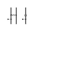
Figure 1: Feynman diagrams representing the one-photon-exchange correction to the $g$ factor in the framework of the extended Furry picture. The wavy line indicates the photon propagator. The triple line represents the electron propagator in the effective potential $V_{\rm eff}$. The dashed line terminated with the triangle corresponds to the interaction with external magnetic field. The symbol $\otimes$ represents the screening potential counterterm.

Within the framework of bound-state QED, each term of the perturbation theory is represented by the corresponding set of diagrams. Currently, there are several methods to derive formal expressions from the first principles of QED: the two-time Green’s function method Shabaev (2002), the covariant-evolution-operator method Lindgren et al. (2004), and the line profile approach O. Yu. Andreev et al. (2008). The corresponding formulas for $\Delta g^{(i)}_{\rm int}$ were derived in Ref. Shabaeva and Shabaev (1995) (first order) and in Ref. Volotka et al. (2012) (second order) within the two-time Green’s function method. The leading correction $\Delta g^{(1)}_{\rm int}$ to the $g$ factor corresponds to the one-photon-exchange diagram in the presence of magnetic field, see Fig. 1. Also the counterterm diagram appears in the presence of the screening potential. This diagram is also shown in Fig. 1, where the symbol $\otimes$ denotes the counterterm. The corresponding expression for the interelectronic-interaction correction reads as:

$$\Delta g^{(1)}_{\mathrm{int}}=\dfrac{1}{m_{a}}\sum_{b}\sum_{P,Q}(-1)^{P+Q}\Bigg{[}2{\sum_{n}}^{\prime}\frac{\langle Pa\,Pb|I(\varepsilon_{Qa}-\varepsilon_{Pa})|n\,Qb\rangle\langle n|U|Qa\rangle}{\varepsilon_{Qa}-\varepsilon_{n}}$$

$$-\langle Pa\,Pb|I^{\prime}(\varepsilon_{Qa}-\varepsilon_{Pa})|Qa\,Qb\rangle\langle Qb|U|Qb\rangle\Bigg{]}-\dfrac{1}{m_{a}}{\sum_{n}}^{\prime}\frac{\langle a|V_{\rm scr}|n\rangle\langle n|U|a\rangle}{\varepsilon_{a}-\varepsilon_{n}}\,.$$ (14)

Here $P$ and $Q$ are permutation operators giving rise to the sign $(-1)^{P+Q}$ according to the parity of the permutation, $\varepsilon_{n}$ are the one-electron energies, $|b\rangle$ stands for the $1s$ state, while the summation over $b$ runs over two possible projections $m_{b}=\pm 1/2$. The prime on the sums over the intermediate states $n$ denotes that the terms with vanishing denominators are omitted.

The interelectronic-interaction operator $I(\omega)$ in the Feynman gauge is given by

$$I(\omega,r_{12})=\alpha(1-\bm{\alpha}_{1}\cdot\bm{\alpha}_{2})\dfrac{\exp{(i\tilde{\omega}r_{12})}}{r_{12}}\,.$$ (15)

In the Coulomb gauge it is given by

$$I(\omega,r_{12})=\alpha\left(\dfrac{1}{r_{12}}-\bm{\alpha}_{1}\cdot\bm{\alpha}_{2}\dfrac{\exp{(i\tilde{\omega}r_{12})}}{r_{12}}-\left[\bm{\alpha}_{1}\cdot\bm{\nabla}_{1},\left[\bm{\alpha}_{2}\cdot\bm{\nabla}_{2},\dfrac{\exp{(i\tilde{\omega}r_{12})}-1}{\omega^{2}r_{12}}\right]\right]\right)\,.$$ (16)

Here $r_{12}=|{\bf r}_{1}-{\bf r}_{2}|$, and $\tilde{\omega}=\sqrt{\omega^{2}+i0}$, the branch of the square root is fixed by the condition ${\rm Im}\,\tilde{\omega}>0$. In Eq. (III.1) the notation $I^{\prime}(\omega)=dI(\omega)/d\omega$ is used.

Assuming $\omega=0$ in the Coulomb gauge we obtain $I$ in the Breit approximation,

$$I_{\rm B}(r_{12})=\alpha\left(\dfrac{1}{r_{12}}-\frac{\bm{\alpha}_{1}\cdot\bm{\alpha}_{2}}{r_{12}}+\frac{1}{2}\left[\bm{\alpha}_{1}\cdot\bm{\nabla}_{1},\left[\bm{\alpha}_{2}\cdot\bm{\nabla}_{2},r_{12}\right]\right]\right)\,.$$ (17)

This form is used to calculate the third- and higher-order contributions, see Sec. III.3.

III.2 Second-order contribution

The second-order correction $\Delta g^{(2)}_{\rm int}$ corresponds to the two-photon-exchange diagrams which can be divided into two large classes, namely three-electron (Fig. 2) and two-electron (Fig. 3) ones. In the extended Furry picture, the counterterm diagrams shown in Fig. 4 appear in addition. The contributions of these diagrams are divided into reducible and irreducible parts. Reducible part is the contributions in which the energies of the intermediate and reference states coincide, while the irreducible part is the remainder. The reducible part is taken together with the non-diagrammatic perturbation-theory terms of the corresponding order.

So, the second-order correction $\Delta g^{(2)}_{\rm int}$ to the $g$ factor can be written as follows,

$$\Delta g^{(2)}_{\rm int}=\Delta g^{(2)}_{\rm 3el}+\Delta g^{(2)}_{\rm 2el}+\Delta g^{(2)}_{\rm ct}+\Delta g^{(2)}_{\rm red}\,.$$ (18)

The three-electron contribution $\Delta g^{(2)}_{\rm 3el}$ can be written as the sum,

$$\Delta g^{(2)}_{\rm 3el}=\Delta g^{(2)}_{\rm 3el,A}+\Delta g^{(2)}_{\rm 3el,B}+\Delta g^{(2)}_{\rm 3el,C}+\Delta g^{(2)}_{\rm 3el,D}\,,$$ (19)

where each term is the irreducible part of the corresponding Feynman diagram in Fig. 2. The formal expressions for $\Delta g^{(2)}_{\rm 3el}$ can be found in Appendix Three-electron contribution, they involve double summation over the Dirac spectrum. The two-electron contribution $\Delta g^{(2)}_{\rm 2el}$, in contrast to the $\Delta g^{(2)}_{\rm 3el}$, comprises triple summation and the integration over the virtual photon energy $\omega$, thus making its evaluation significantly more involved, including development of the numerical procedure. Similarly to Eq. (19), we represent it in the following form,

$$\Delta g^{(2)}_{\rm 2el}=\Delta g^{(2)}_{\rm 2el,lad-W}+\Delta g^{(2)}_{\rm 2el,lad-S}+\Delta g^{(2)}_{\rm 2el,cr-W}+\Delta g^{(2)}_{\rm 2el,cr-S}\,.$$ (20)

This contribution consist of ladder (“lad”) and cross (“cr”) parts, see Fig. 3, which are named by analogy with the two-photon-exchange diagrams without the external-field vertex Shabaev (2002), the labels “W” and “S” indicate the position of this vertex. The formal expressions for these terms can be found in Appendix Two-electron contribution.

The third term $\Delta g^{(2)}_{\rm red}$ in Eq. (18) includes the reducible parts of all diagrams, both two-electron and three-electron, including the non-diagrammatic terms, see Appendix Reducible contribution. Finally, the counterterm contribution $\Delta g^{(2)}_{\rm ct}$ corresponds to the diagrams in Fig. 4 which arise when the screening potential is included in the Dirac equation.

Figure 2: Feynman diagrams representing the three-electron part of the two-photon-exchange correction to the $g$ factor in the framework of the extended Furry picture. Notations are the same as in Fig. 1.

Figure 3: Feynman diagrams representing the two-electron part of the two-photon-exchange correction to the $g$ factor in the framework of the extended Furry picture. Notations are the same as in Fig. 1.

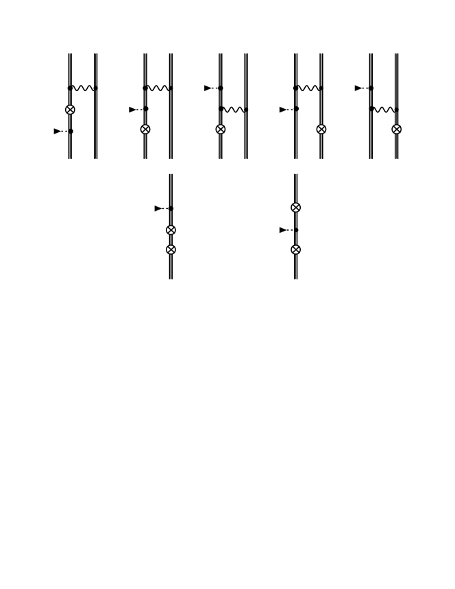
Figure 4: Feynman diagrams representing the counterterm part of the two-photon-exchange correction to the $g$ factor in the framework of the extended Furry picture. Notations are the same as in Fig. 1.

Table 1: Individual contributions to the two-photon-exchange correction for the ground-state $g$ factor of ²⁸Si¹¹⁺ and ²⁰⁸Pb⁷⁹⁺ obtained for the core-Hartree potential in the Feynman and Coulomb gauges.

	28Si11+		208Pb79+
Contribution	Feynman	Coulomb	Feynman	Coulomb
3el, A	$-35.5174$	$-32.1510$	$-47.5059$	$-57.4179$
3el, B	$39.5459$	$36.1787$	$50.7785$	$60.6392$
3el, C	$19\,540.5865$	$19\,537.1073$	$625.5797$	$621.2035$
3el, D	$-96.6335$	$-96.2590$	$-120.4084$	$-122.3388$
2el, lad-W	$-13\,638.4718$	$-13\,663.2943$	$-3016.6610$	$-3054.2046$
2el, cr-W	$-83.2577$	$-60.5589$	$-2679.1832$	$-2648.0997$
2el, lad-S	$20\,478.7090$	$20\,571.8104$	$606.4759$	$614.7309$
2el, cr-S	$22.9387$	$-0.4702$	$12.8076$	$-1.0717$
red, E	$-19\,546.8105$	$-19\,543.7536$	$-627.3047$	$-622.8958$
red, F	$234.1531$	$234.2034$	$296.3070$	$298.5116$
red, G	$0.9138$	$-0.0331$	$0.7037$	$-1.6609$
red, 2el	$-6923.7189$	$-6990.3424$	$4889.2411$	$4903.4344$
ct-1	$18.6909$	$18.6909$	$20.0834$	$20.0834$
ct-2	$-10.9920$	$-10.9920$	$-11.0497$	$-11.0497$
Total	$0.1362(1)$	$0.1362(1)$	$-0.1361(1)$	$-0.1361(1)$

III.3 Higher-order contribution

Rigorous evaluation of the higher-order term $\Delta g^{(3+)}_{\rm int}$ to all orders in $\alpha Z$ is not feasible at the moment. In this case, one of the currently available methods Bratzev et al. (1977); Dzuba et al. (1987); Blundell et al. (1989); Shabaev et al. (1995); Boucard and Indelicato (2000); Zherebtsov and Shabaev (2000); Yerokhin (2008); Ginges and Volotka (2018) can be considered. The all-order CI-DFS method Bratzev et al. (1977) was employed in Refs. Glazov et al. (2004, 2005) to find the contribution of the second and higher orders. In Ref. Volotka et al. (2014) the two-photon-exchange diagrams were evaluated within the rigorous QED approach, and thus only $\Delta g^{(3+)}_{\rm int}$ was needed from the CI-DFS calculations. This was a demanding task since the subtraction of the leading orders from the total value delivered by any all-order method requires high enough numerical accuracy. In this paper, we use the recursive formulation of perturbation theory Glazov et al. (2017), which provides an efficient way to accesses the individual terms of the perturbation expansion up to any order, in principle. Application of this method to the $g$ factor of lithiumlike silicon and calcium in Refs. Glazov et al. (2019); Kosheleva et al. (2022) has demonstrated the ability to provide significantly better accuracy than the CI-DFS method. Recently, non-relativistic quantum electrodynamics (NRQED) approach was used to solve this task with even better accuracy Yerokhin et al. (2020, 2021). At the same time, perturbation theory allows one to include screening potential which is an important ingredient here Kosheleva et al. (2022), while the NRQED calculations were based on the Coulomb potential so far.

To formulate our approach, we start with the Dirac-Coulomb-Breit equation,

$$\Lambda_{+}\left(H_{0}+H_{1}\right)\Lambda_{+}|A\rangle=E_{A}|A\rangle\,,$$ (21)

where $\Lambda_{+}$ is the projection operator constructed as the product of one-electron projectors on the positive energy states. Zeroth-order Hamiltonian $H_{0}$ is the sum of the one-electron Dirac Hamiltonians,

$$H_{0}=\sum_{j}h^{\rm D}(j)\,,$$ (22)

where $h^{\rm D}$ is given by Eq. (3).

Let us introduce the zeroth-order eigenfunctions $N^{(0)}$ as

$$\Lambda_{+}H_{0}\Lambda_{+}|N^{(0)}\rangle=E_{N}^{(0)}|N^{(0)}\rangle\,.$$ (23)

These functions form an orthogonal basis set of many-electron wave functions. In our case, they are constructed as the Slater determinants of one-electron solutions of the Dirac equation. In particular, for the reference state $|A\rangle$ in the zeroth approximation we have

$$\Lambda_{+}H_{0}\Lambda_{+}|A^{(0)}\rangle=E_{A}^{(0)}|A^{(0)}\rangle\,.$$ (24)

The perturbation $H_{1}$ in (21) reads as

$$H_{1}=\,\sum_{j<k}I_{\rm B}(j,k)-\sum_{j}V_{\rm scr}(j)\,,$$ (25)

and represents the interelectronic interaction in the Breit approximation with the screening potential subtracted.

We use the perturbation theory with respect to $H_{1}$, which yields the following expansions for the energy $E_{A}$ and the wave function $|A\rangle$,

$$E_{A} =\sum_{k=0}^{\infty}E_{A}^{(k)}\,,$$ (26)

$$|A\rangle =\sum_{k=0}^{\infty}|A^{(k)}\rangle=\sum_{k=0}^{\infty}\sum_{N}|N^{(0)}\rangle\langle N^{(0)}|A^{(k)}\rangle\,.$$ (27)

In Ref. Glazov et al. (2017) the recursive scheme to evaluate $E_{A}^{(k)}$ and $\langle N^{(0)}|A^{(k)}\rangle$ order by order was presented. We emphasize that instead of the widely used normalization $\langle A^{{(0)}}|A\rangle=1$, we impose the condition $\langle A|A\rangle=1$. Below we consider how to use this method to find the interelectronic-interaction contributions $\Delta g_{\rm int}^{(k)}$.

For the many-electron state $|A\rangle$ the $g$ factor is found as

$$g=\dfrac{1}{m_{a}}\langle A|\sum_{i}U(i)|A\rangle\,,$$ (28)

and in the zeroth approximation with $|A^{(0)}\rangle$, this expression reduces to Eq. (4). Substituting the expansion (27) we find the term of the order $k\geq 1$ as

$$\Delta g_{\rm int}^{(k)}[+] =\dfrac{1}{m_{a}}\,\sum_{j=0}^{k}\langle A^{(j)}|\sum_{i}U(i)|A^{(k-j)}\rangle$$

$$=\dfrac{1}{m_{a}}\,\sum_{j=0}^{k}\sum_{M,N}\langle A^{(j)}|M^{(0)}\rangle\langle M^{(0)}|\sum_{i}U(i)|N^{(0)}\rangle\langle N^{(0)}|A^{(k-j)}\rangle\,.$$ (29)

In fact, Eq. (III.3) yields the contribution of the positive-energy states only, since only positive-energy excitation are included in the expansion (27). For this reason, we label the result with “$[+]$” sign. However, the negative-energy spectrum is equally important, see e.g. Refs. Glazov et al. (2004); Maison et al. (2019). Its contribution is given by the following expression,

$$\Delta g_{\rm int}[-]=\dfrac{2}{m_{a}}\,\sum_{p,n}\frac{\langle p|U|n\rangle}{\varepsilon_{p}-\varepsilon_{n}}\langle\hat{a}^{+}_{n}\hat{a}_{p}A|H_{1}|A\rangle\,.$$ (30)

Here $|p\rangle$ and $|n\rangle$ are the positive- and negative-energy one-electron states, respectively, $\hat{a}^{+}$ and $\hat{a}$ are the corresponding creation and annihilation operators. The term of the order $k$ reads,

$$\Delta g_{\rm int}^{(k)}[-]=\dfrac{2}{m_{a}}\,\sum_{j=0}^{k-1}\sum_{M,N}\langle A^{(j)}|M^{(0)}\rangle\left[\sum_{p,n}\frac{\langle p|U|n\rangle\langle\hat{a}^{+}_{n}\hat{a}_{p}M^{(0)}|H_{1}|N^{(0)}\rangle}{\varepsilon_{p}-\varepsilon_{n}}\right]\langle N^{(0)}|A^{(k-j-1)}\rangle\,.$$ (31)

The equations (III.3) and (31) provide the interelectronic-interaction contributions within the Breit approximation,

$$\Delta g_{\rm int,\rm L}^{(k)}=\Delta g_{\rm int}^{(k)}[+]+\Delta g_{\rm int}^{(k)}[-]\,.$$ (32)

The complete $k$-order terms can be presented in the following form,

$$\Delta g^{(k)}_{\rm int}=\Delta g^{(k)}_{\rm int,\rm L}+\Delta g^{(k)}_{\rm int,\rm H}\,,$$ (33)

where $\Delta g^{(k)}_{\rm int,\rm H}$ is the presently unknown higher-order part, which has to be estimated somehow to ascribe the uncertainty to $\Delta g^{(k)}_{\rm int}$. In the present work, $\Delta g^{(3+)}_{\rm int,\rm H}$ is estimated as $\pm 2\Delta g^{(2)}_{\rm int,\rm H}/Z$, as proposed in our previous work Kosheleva et al. (2022).

Table 2: Interelectronic-interaction contributions $\Delta g^{(k)}_{\rm int,\rm L}$ to the ground-state $g$ factor of ²⁸Si¹¹⁺, in units of $10^{-6}$. The results are obtained in the Breit approximation with the Coulomb and different screening potentials: core-Hartree (CH), Kohn-Sham (KS), Dirac-Hartree (DH), and Dirac-Slater (DS). The last three are considered with (marked by superscript L) and without the Latter correction.

$k$	Coul	CH	KS	$\mathrm{KS^{L}}$	DH	$\mathrm{DH^{L}}$	DS	$\mathrm{DS^{L}}$
$0$		$348.266\,78$	$341.443\,36$	$341.368\,2$	$417.198\,16$	$353.163\,8$	$302.709\,55$	$329.110\,2$
$1$	$321.437\,11$	$-33.663\,23$	$-25.289\,06$	$-25.211(1)$	$-104.409\,66$	$-39.393(1)$	$14.546\,44$	$-11.879(1)$
$2$	$-6.825\,89(4)$	$0.146\,64(3)$	$-1.480\,24(3)$	$-1.471\,8(2)$	$2.102\,45(3)$	$1.132\,6(3)$	$-2.645\,79(3)$	$-2.576\,6(2)$
$3$	$0.107\,7(41)$	$-0.046\,9(12)$	$0.034\,3(22)$	$0.022\,4(14)$	$-0.197\,8(22)$	$-0.219\,2(10)$	$0.100\,1(23)$	$0.053\,5(13)$
$4$	$-0.013\,13(93)$	$0.004\,65(43)$	$-0.001\,42(40)$	$-0.001\,90(23)$	$0.016\,18(30)$	$0.026\,95(73)$	$-0.004\,33(19)$	$-0.003\,68(39)$
$5$	$0.001\,12(20)$	$-0.000\,12(14)$	$0.000\,09(5)$	$0.000\,08(10)$	$-0.001\,65(16)$	$-0.003\,16(15)$	$-0.000\,15(5)$	$-0.000\,21(5)$
Total	$314.706\,9(42)$	$314.707\,8(13)$	$314.707\,0(22)$	$314.706(2)$	$314.707\,7(22)$	$314.708(2)$	$314.705\,8(23)$	$314.704(2)$

IV RESULTS AND DISCUSSIONS

In this section we discuss the numerical evaluation of all the considered contributions to $\Delta g_{\mathrm{int}}$ and present the results for lithiumlike ions. All calculations are based on the dual-kinetically-balanced finite-basis-set method Shabaev et al. (2004) for the Dirac equation with the basis functions constructed from B-splines Sapirstein and Johnson (1996). First, the Dirac equation (3) is solved with one of the considered potentials. Zeroth-order contribution $\Delta g^{(0)}_{\mathrm{int}}$ is then found according to Eq. (13). Evaluation of $\Delta g^{(1)}_{\mathrm{int}}$ was first accomplished in Ref. Shabaev et al. (2002) and then became a routine procedure Glazov et al. (2004); Volotka et al. (2014); Yerokhin et al. (2017); Glazov et al. (2019); Cakir et al. (2020); Kosheleva et al. (2022). In this work, we calculate it according to Eq. (III.1) with the chosen screening potentials to a required accuracy, using the comparison between the Feynman and Coulomb gauges as an additional crosscheck.

The second-order correction $\Delta g^{(2)}_{\mathrm{int}}$ is calculated according to Eqs. (18), (19), (20), and the formulas from Appendix, which involve double and triple summations over the intermediate states. The number of basis functions is increased up to $N=210$ to achieve clear convergence pattern of the results and then the extrapolation $N\rightarrow\infty$ is performed. The partial wave summation over the relativistic angular quantum number $\kappa=(j+1/2)^{j+l+1/2}$ was terminated at $|\kappa_{\rm max}|=16$ and the remainder was estimated using least-squares inverse polynomial fitting. Moreover, two-electron contributions involve integration over the virtual photon energy $\omega$, which requires special attention due to the poles and cuts from the electron and photon propagators. We use the integration contour proposed in Ref. Mohr and Sapirstein (2000) based on a Wick rotation. The number of the integration points is varied to achieve the required accuracy.

For a consistency check, the two-photon exchange correction is calculated within the Feynman and Coulomb gauges, and the difference between the results is found to be well within the numerical uncertainty. The gauge invariance is demonstrated in Table 1, where the individual terms and the total $\Delta g^{(2)}_{\mathrm{int}}$ values for ²⁸Si¹¹⁺ and ²⁰⁸Pb⁷⁹⁺ obtained with the core-Hartree potential are presented.

Calculations of the third and higher orders $\Delta g^{(3+)}_{\rm int}$ are carried out within the Breit approximation using Eqs. (III.3) and (31). On the one hand, these calculations are rather complicated and time-consuming. On the other hand, the higher the order $k$ the smaller $|\Delta g^{(k)}_{\rm int}|$. Therefore these contributions are required with lower relative accuracy and the corresponding $N$ and $|\kappa_{\rm max}|$ are taken much smaller than for the first and second orders. This is an important advantage of the perturbation theory as compared to CI-DFS and other all-order methods. In particular, to achieve the same accuracy as done here within the CI-DFS method, one would need to calculate the matrix element (28) to ten digits.

The convergence of the perturbation theory is illustrated in Table 2, where the Breit-approximation values of $\Delta g^{(k)}_{\rm int}$ with $k=0\dots 5$ are given for the ground-state $g$ factor of lithiumlike silicon. Calculations are carried out for the Coulomb, core-Hartree and six different DFT potentials: with ($\mathrm{KS^{L}}$, $\mathrm{DH^{L}}$, and $\mathrm{DS^{L}}$) and without (KS, DH, and DS) the Latter correction. Note that the KS, DH, and DS potentials in Ref. Kosheleva et al. (2022) are with the Latter correction, so those values would be placed in the “L” columns. It can be seen that the results without the Latter correction for the one- and two-photon exchange are at least an order of magnitude more accurate than with it. The Latter correction causes the unsmoothness of potentials, which leads to numerical instability. At the same time, all the total values are in agreement within the uncertainties. So, we choose to opt out of the Latter correction in the following.

In Table 3 we present the interelectronic-interaction contributions $\Delta g_{\rm int}$ to the ground-state $g$ factor of lithiumlike ions for $Z=14,54,82$. The results are obtained with the Coulomb and different screening potentials: core-Hartree (CH), Kohn-Sham (KS), Dirac-Hartree (DH), and Dirac-Slater (DS). As seen from this Table, the total values obtained at different screening potentials are quite close to each other and overlap within their uncertainties.

Table 4 shows the values of the interelectronic-interaction correction $\Delta g_{\rm int}$ to the $g$ factor of lithiumlike ions for $Z=14$ – $82$. We have chosen the CH potential here since it is defined unambiguously in contrast to the DFT potentials. For comparison, the values from Refs. Volotka et al. (2014); Yerokhin et al. (2021) are given. As one can see, we have improved the accuracy by an order of magnitude as compared to Volotka et al. (2014). The disagreement with the Coulomb-potential results of Yerokhin et al. (2021) awaits further investigation. The uncertainty of the total values is mainly determined by the numerical error of $\Delta g^{(3+)}_{\text{int,L}}$ and by estimation of unknown $\Delta g^{(3+)}_{\text{int,H}}$. The former is obtained by analyzing the dependence of the results on the basis size. The latter is found as $\pm 2\Delta g^{(2)}_{\rm int,\rm H}/Z$.

Table 3: Interelectronic-interaction contributions to the $g$ factor of ²⁸Si¹¹⁺, ¹³²Xe⁵¹⁺, and ²⁰⁸Pb⁷⁹⁺ ions obtained in the Coulomb and different screening potentials: core-Hartree (CH), Kohn-Sham (KS), Dirac-Hartree (DH), and Dirac-Slater (DS) (all without the Latter correction), in units of $10^{-6}$.

	Coulomb	CH	KS	DH	DS
$Z=14$
$\Delta g^{(0)}_{\rm int}$		$348.2661$	$341.4434$	$417.1982$	$302.7096$
$\Delta g_{\rm int}^{(1)}$	$321.5903$	$-33.5491$	$-25.1729$	$-104.3024$	$14.6672$
$\Delta g_{\rm int}^{(2)}$	$-6.8782(1)$	$0.1362(1)$	$-1.4929(1)$	$2.0986(1)$	$-2.6630(1)$
	$-6.8787(1)$a
$\Delta g^{(3+)}_{\text{int,L}}$	$0.0934(21)$	$-0.0443(10)$	$0.0330(22)$	$-0.1833(22)$	$0.0956(23)$
$\Delta g^{(3+)}_{\text{int,H}}$	$0.0000(74)$	$0.0000(14)$	$0.0000(18)$	$0.0000(5)$	$0.0000(25)$
	$0.0000(14)$a
Total	$314.8055(77)$	$314.8089(17)$	$314.8106(28)$	$314.8111(23)$	$314.8094(34)$
	$314.8058(15)$a
$Z=54$
$\Delta g^{(0)}_{\rm int}$		$1463.1608$	$1414.1410$	$1763.0709$	$1238.6240$
$\Delta g_{\rm int}^{(1)}$	$1306.2170$	$-164.6779$	$-113.4828$	$-466.1252$	$63.4535$
$\Delta g_{\rm int}^{(2)}$	$-7.6565(3)$	$0.1376(2)$	$-2.0667(1)$	$1.7041(1)$	$-3.5117(1)$
	$-7.6569(5)$a
$\Delta g^{(3+)}_{\text{int,L}}$	$0.0308(22)$	$-0.0106(19)$	$0.0174(10)$	$-0.0354(17)$	$0.0417(9)$
$\Delta g^{(3+)}_{\text{int,H}}$	$0.0000(255)$	$0.0000(74)$	$0.0000(81)$	$0.0000(41)$	$0.0000(101)$
Total	$1298.5913(256)$	$1298.6099(76)$	$1298.6089(82)$	$1298.6144(44)$	$1298.6075(101)$
$Z=82$
$\Delta g^{(0)}_{\rm int}$		$2448.8325$	$2341.3605$	$2952.7350$	$2034.2466$
$\Delta g_{\rm int}^{(1)}$	$2148.2959$	$-309.3425$	$-198.8050$	$-814.6876$	$110.2598$
$\Delta g_{\rm int}^{(2)}$	$-8.9897(5)$	$-0.1361(1)$	$-3.2341(1)$	$1.3279(1)$	$-5.2159(1)$
	$-8.9905(6)$a
$\Delta g^{(3+)}_{\text{int,L}}$	$0.0459(24)$	$-0.0057(31)$	$0.0232(27)$	$-0.0237(23)$	$0.0564(14)$
$\Delta g^{(3+)}_{\text{int,H}}$	$0.0000(283)$	$0.0000(122)$	$0.0000(115)$	$0.0000(86)$	$0.0000(130)$
Total	$2139.3521(284)$	$2139.3482(126)$	$2139.3446(118)$	$2139.3516(89)$	$2139.3469(131)$

^a Yerokhin et al. (2021) Yerokhin et al. (2021)

Table 4: Interelectronic-interaction contributions to the $g$ factor of lithiumlike ions with $Z=14$ – $82$ obtained for the core-Hartree (CH) potential, in units of $10^{-6}$.

$Z$	$\Delta g^{(0)}_{\rm int}$	$\Delta g^{(1)}_{\rm int}$	$\Delta g^{(2)}_{\rm int}$	$\Delta g^{(3+)}_{\text{int,L}}$	$\Delta g^{(3+)}_{\text{int,H}}$	Total
14	$348.2661$	$-33.5491$	$0.1362(1)$	$-0.0443(10)$	$0.0000(14)$	$314.8089(17)$
	$348.267$a	$-33.549$a	$0.137$a	$-0.046(6)$a		$314.809(6)$a
						$314.8058(15)$b
18	$452.6955$	$-45.1729$	$0.1301(1)$	$-0.0318(12)$	$0.0000(20)$	$407.6209(23)$
20	$505.2339$	$-51.0429$	$0.1291(1)$	$-0.0300(8)$	$0.0000(24)$	$454.2902(25)$
	$505.234$a	$-51.042$a	$0.129$a	$-0.031(9)$a		$454.290(9)$a
						$454.2834(25)$b
24	$611.0988$	$-62.9331$	$0.1300(1)$	$-0.0239(17)$	$0.0000(29)$	$548.2718(34)$
32	$826.7992$	$-87.5079$	$0.1371(1)$	$-0.0185(13)$	$0.0000(40)$	$739.4099(42)$
40	$1049.4869$	$-113.5613$	$0.1451(1)$	$-0.0147(13)$	$0.0000(57)$	$936.0560(58)$
54	$1463.1608$	$-164.6779$	$0.1376(2)$	$-0.0106(19)$	$0.0000(74)$	$1298.6099(76)$
70	$1991.9926$	$-237.5105$	$0.0466(1)$	$-0.0090(24)$	$0.0000(100)$	$1754.520(10)$
82	$2448.8325$	$-309.3425$	$-0.1361(1)$	$-0.0057(31)$	$0.0000(122)$	$2139.348(13)$
	$2448.833$a	$-309.340$a	$-0.134$a	$-0.015(10)$a	$0.000(40)$a	$2139.34(4)$a

^a Volotka et al. (2014) Volotka et al. (2014); ^b Yerokhin et al. (2021) Yerokhin et al. (2021).

V CONCLUSION

In conclusion, the electron correlation effects on the $g$ factor of lithiumlike ions in the range $Z=14-82$ are evaluated with an uncertainty on the level of $10^{-6}$. The first- and second-order interelectronic-interaction corrections are calculated within the rigorous bound-state QED approach, i.e., to all orders in $\alpha Z$. The third- and higher-order contributions are taken into account within the Breit approximation using the recursive perturbation theory. In comparison to previous theoretical calculations, the accuracy of the interelectronic-interaction contributions to the bound-electron $g$ factor in lithiumlike ions is substantially improved.

APPENDIX: QED formulas for two-photon-exchange contribution

In this Appendix we present the explicit formulas for the two-photon-exchange contribution to the $g$ factor of lithiumlike ions derived within the two-time Green’s function method Shabaev (2002). We separate the irreducible contributions of the two- and three-electron diagrams, the reducible contribution, including the non-diagrammatic terms, and the counterterm contribution, see Eq. (18).

Three-electron contribution

The three-electron contribution to the two-photon-exchange correction, see Fig. 2, is given by the sum, according to the types of diagrams in Fig. 2,

$$\Delta g^{(2)}_{\rm 3el}=\Delta g^{(2)}_{\rm 3el,A}+\Delta g^{(2)}_{\rm 3el,B}+\Delta g^{(2)}_{\rm 3el,C}+\Delta g^{(2)}_{\rm 3el,D}\,,$$ (34)

where

$$\Delta g^{(2)}_{\rm 3el,A}=\frac{1}{m_{a}}\sum_{b_{1},b_{2}}\sum_{P,Q}(-1)^{P+Q}{\sum_{n}}^{\prime}\frac{\langle PaPb_{1}|I(\Delta_{PaQa})|\xi_{Qa}n\rangle\langle nPb_{2}|I(\Delta_{Pb_{2}Qb_{2}})|Qb_{1}Qb_{2}\rangle}{\varepsilon_{Pa}+\varepsilon_{Pb_{1}}-\varepsilon_{Qa}-\varepsilon_{n}}\,,$$ (35)

$$\Delta g^{(2)}_{\rm 3el,B}=\frac{1}{m_{a}}\sum_{b_{1},b_{2}}\sum_{P,Q}(-1)^{P+Q}{\sum_{n}}^{\prime}\frac{\langle\xi_{Pa}Pb_{1}|I(\Delta_{PaQa})|Qan\rangle\langle nPb_{2}|I(\Delta_{Pb_{2}Qb_{2}})|Qb_{1}Qb_{2}\rangle}{\varepsilon_{Pa}+\varepsilon_{Pb_{1}}-\varepsilon_{Qa}-\varepsilon_{n}}\,,$$ (36)

$$\Delta g^{(2)}_{\rm 3el,C} = \frac{1}{2m_{a}}\sum_{b_{1},b_{2}}\sum_{P,Q}(-1)^{P+Q}$$ (37)

$$\times {\sum_{n_{1},n_{2}}}^{\prime}\frac{\langle PaPb_{1}|I(\Delta_{PaQa})|Qan_{1}\rangle\langle n_{1}|U|n_{2}\rangle\langle n_{2}Pb_{2}|I(\Delta_{Pb_{2}Qb_{2}})|Qb_{1}Qb_{2}\rangle}{(\varepsilon_{Pa}+\varepsilon_{Pb_{1}}-\varepsilon_{Qa}-\varepsilon_{n_{1}})(\varepsilon_{Qb_{1}}+\varepsilon_{Qb_{2}}-\varepsilon_{Pb_{2}}-\varepsilon_{n_{2}})}\,,$$

$$\Delta g^{(2)}_{\rm 3el,D}=\frac{1}{m_{a}}\sum_{b_{1},b_{2}}\sum_{P,Q}(-1)^{P+Q}{\sum_{n}}^{\prime}\frac{\langle Pa\xi_{Pb_{1}}|I(\Delta_{PaQa})|Qan\rangle\langle nPb_{2}|I(\Delta_{Pb_{2}Qb_{2}})|Qb_{1}Qb_{2}\rangle}{\varepsilon_{Pa}+\varepsilon_{Pb_{1}}-\varepsilon_{Qa}-\varepsilon_{n}}\,,$$ (38)

where

$$|\xi_{c}\rangle={\sum_{n}}^{\prime}\frac{|n\rangle\langle n|U|c\rangle}{\varepsilon_{c}-\varepsilon_{n}}\,,$$ (39)

the prime over the sums means that terms with vanishing denominators should be omitted in the summation, $P$ and $Q$ are permutation operators, which determine the sign $(-1)^{P+Q}$, $\Delta_{PaQb}=\varepsilon_{Pa}-\varepsilon_{Qb}$.

Two-electron contribution

The irreducible parts of the two-electron diagrams depicted in Fig. 3 yield

$$\Delta g^{(2)}_{\rm 2el}=\Delta g^{(2)}_{\rm 2el,lad-W}+\Delta g^{(2)}_{\rm 2el,lad-S}+\Delta g^{(2)}_{\rm 2el,cr-W}+\Delta g^{(2)}_{\rm 2el,cr-S}\,,$$ (40)

with

$$\Delta g^{(2)}_{\rm 2el,lad-W} = \frac{1}{m_{a}}\sum_{b}\sum_{P,Q}(-1)^{P+Q}\frac{i}{\pi}\int_{-\infty}^{\infty}{\rm d}\omega$$ (41)

$$\times {\sum_{n_{1},n_{2}}}^{\prime}\,\frac{\langle PaPb|I(\omega)|n_{1}n_{2}\rangle\langle n_{1}n_{2}|I(\omega+\Delta_{PaQa})|\xi_{Qa}Qb\rangle}{(\varepsilon_{Pa}+\omega-u\varepsilon_{n_{1}})(\varepsilon_{Qb}-\omega-\Delta_{PaQa}-u\varepsilon_{n_{2}})}\,,$$

$$\Delta g^{(2)}_{\rm 2el,lad-S} = \frac{1}{m_{a}}\sum_{b}\sum_{P,Q}(-1)^{P+Q}\frac{i}{2\pi}\int_{-\infty}^{\infty}{\rm d}\omega$$ (42)

$$\times {\sum_{n_{1},n_{2},n_{3}}}^{\prime}\,\frac{\langle PaPb|I(\omega)|n_{1}n_{2}\rangle\langle n_{2}|U|n_{3}\rangle\langle n_{1}n_{3}|I(\omega+\Delta_{PaQa})|QaQb\rangle}{(\varepsilon_{Pa}+\omega-u\varepsilon_{n_{1}})(\varepsilon_{Qb}-\omega-\Delta_{PaQa}-u\varepsilon_{n_{2}})(\varepsilon_{Qb}-\omega-\Delta_{PaQa}-u\varepsilon_{n_{3}})}\,,$$

$$\Delta g^{(2)}_{\rm 2el,cr-W} = \frac{1}{m_{a}}\sum_{b}\sum_{P,Q}(-1)^{P+Q}\frac{i}{\pi}\int_{-\infty}^{\infty}{\rm d}\omega$$ (43)

$$\times {\sum_{n_{1},n_{2}}}^{\prime}\,\frac{\langle Pan_{2}|I(\omega)|n_{1}Qb\rangle\langle\xi_{Pb}n_{1}|I(\omega-\Delta_{PaQa})|n_{2}Qa\rangle}{(\varepsilon_{Pa}-\omega-u\varepsilon_{n_{1}})(\varepsilon_{Qb}-\omega-u\varepsilon_{n_{2}})}\,,$$

$$\Delta g^{(2)}_{\rm 2el,cr-S} = \frac{1}{m_{a}}\sum_{b}\sum_{P,Q}(-1)^{P+Q}\frac{i}{2\pi}\int_{-\infty}^{\infty}{\rm d}\omega$$ (44)

$$\times {\sum_{n_{1},n_{2},n_{3}}}^{\prime}\,\frac{\langle Pan_{2}|I(\omega)|n_{1}Qb\rangle\langle n_{3}|U|n_{2}\rangle\langle Pbn_{1}|I(\omega-\Delta_{PaQa})|n_{3}Qa\rangle}{(\varepsilon_{Pa}-\omega-u\varepsilon_{n_{1}})(\varepsilon_{Qb}-\omega-u\varepsilon_{n_{2}})(\varepsilon_{Qb}-\omega-u\varepsilon_{n_{3}})}\,,$$

where the prime on the sums indicates that in the summation we omit the reducible and infrared-divergent terms, namely, those with $\varepsilon_{n_{1}}+\varepsilon_{n_{2}}=\varepsilon_{a}+\varepsilon_{b}$ in the ladder-W diagrams, with $\varepsilon_{n_{1}}=\varepsilon_{Pa},\,\varepsilon_{n_{2}}=\varepsilon_{Qb}$ in the direct parts of the cross-W diagrams and $\varepsilon_{n_{1}}=\varepsilon_{n_{2}}=\varepsilon_{a},\varepsilon_{b}$ in the exchange parts of the cross-W diagrams, with $\varepsilon_{n_{1}}+\varepsilon_{n_{2}}=\varepsilon_{a}+\varepsilon_{b}$, $\varepsilon_{n_{1}}+\varepsilon_{n_{3}}=\varepsilon_{a}+\varepsilon_{b}$, and $\varepsilon_{n_{2}}=\varepsilon_{n_{3}}=\varepsilon_{Qb}-\Delta_{PaQa}$ in the ladder-S diagrams, with $\varepsilon_{n_{1}}=\varepsilon_{Pa},\,\varepsilon_{n_{2}}=\varepsilon_{Qb}$, $\varepsilon_{n_{1}}=\varepsilon_{Pa},\,\varepsilon_{n_{3}}=\varepsilon_{Qb}$, and $\varepsilon_{n_{2}}=\varepsilon_{n_{3}}=\varepsilon_{Qb}$ in the direct parts of the cross-S diagrams, with $\varepsilon_{n_{1}}=\varepsilon_{n_{2}}=\varepsilon_{a},\varepsilon_{b}$, $\varepsilon_{n_{1}}=\varepsilon_{n_{3}}=\varepsilon_{a},\varepsilon_{b}$, and $\varepsilon_{n_{2}}=\varepsilon_{n_{3}}=\varepsilon_{a},\varepsilon_{b}$ in the exchange parts of the cross-S diagrams. $u=1-i0$ preserves the proper treatment of poles of the electron propagators.

Reducible contribution

The reducible parts of the two-electron diagrams are given by the following expressions,

$$\Delta g^{(2)}_{\rm red}=\Delta g^{(2)}_{\rm red,E}+\Delta g^{(2)}_{\rm red,F}+\Delta g^{(2)}_{\rm red,G}+\Delta g^{(2)}_{\rm red,2el}\,,$$ (45)

where red,E term is given by

$$\Delta g^{(2)}_{\rm red,E}=\Delta g^{(2)}_{\rm red,Ea}+\Delta g^{(2)}_{\rm red,Eb}$$ (46)

with

$$\Delta g^{(2)}_{\rm red,Ea} = \frac{1}{m_{a}}\sum_{b_{1},b_{2}}\sum_{P,Q}(-1)^{P+Q}\langle a|U|a\rangle{\sum_{n}}^{\prime}$$ (47)

$$\times \left\{\frac{1}{2}\frac{\langle Qb_{1}Qb_{2}|I(\Delta_{Qb_{1}a})|an\rangle\langle na|I(\Delta_{aPb_{2}})|Pb_{1}Pb_{2}\rangle}{(2\varepsilon_{b}-\varepsilon_{a}-\varepsilon_{n})^{2}}\right.-\frac{\langle Qb_{1}Qb_{2}|I^{\prime}(\Delta_{Qb_{1}a})|an\rangle\langle na|I(\Delta_{aPb_{2}})|Pb_{1}Pb_{2}\rangle}{2\varepsilon_{b}-\varepsilon_{a}-\varepsilon_{n}}$$

$$+ \frac{\langle Qb_{1}Qa|I(\Delta_{Qb_{1}b_{2}})|b_{2}n\rangle\langle nb_{2}|I(\Delta_{b_{2}Pb_{1}})|PaPb_{1}\rangle}{(\varepsilon_{a}-\varepsilon_{n})^{2}}-2\frac{\langle Qb_{1}Qa|I^{\prime}(\Delta_{Qb_{1}b_{2}})|b_{2}n\rangle\langle nb_{2}|I(\Delta_{b_{2}Pb_{1}})|PaPb_{1}\rangle}{\varepsilon_{a}-\varepsilon_{n}}$$

$$+ \frac{\langle QaQb_{1}|I(\Delta_{Qab_{1}})|b_{1}n\rangle\langle nb_{2}|I(\Delta_{b_{2}Pb_{2}})|PaPb_{2}\rangle}{(\varepsilon_{a}-\varepsilon_{n})^{2}}-2\frac{\langle QaQb_{1}|I^{\prime}(\Delta_{Qab_{1}})|b_{1}n\rangle\langle nb_{2}|I(\Delta_{b_{2}Pb_{2}})|PaPb_{2}\rangle}{\varepsilon_{a}-\varepsilon_{n}}$$

$$- \left.2\frac{\langle QaQb_{2}|I^{\prime}(\Delta_{Qaa})|an\rangle\langle nb_{1}|I(\Delta_{b_{1}Pb_{1}})|Pb_{2}Pb_{1}\rangle}{\varepsilon_{b}-\varepsilon_{n}}\right\}$$

and

$$\Delta g^{(2)}_{\rm red,Eb} = \frac{1}{m_{a}}\sum_{b_{1},b_{2}}\sum_{P,Q}(-1)^{P+Q}\langle b_{2}|U|b_{2}\rangle{\sum_{n}}^{\prime}\left\{\frac{\langle Qb_{2}Qa|I(\Delta_{Qb_{2}b_{1}})|b_{1}n\rangle\langle nb_{1}|I(\Delta_{b_{1}Pb_{2}})|PaPb_{2}\rangle}{(\varepsilon_{a}-\varepsilon_{n})^{2}}\right.$$ (48)

$$+ \frac{\langle Qb_{2}Qb_{1}|I(\Delta_{Qb_{2}a})|an\rangle\langle na|I(\Delta_{aPb_{2}})|Pb_{1}Pb_{2}\rangle}{(2\varepsilon_{b}-\varepsilon_{a}-\varepsilon_{n})^{2}}-\frac{\langle Qb_{2}Qb_{1}|I^{\prime}(\Delta_{Qb_{2}a})|an\rangle\langle na|I(\Delta_{aPb_{2}})|Pb_{1}Pb_{2}\rangle}{2\varepsilon_{b}-\varepsilon_{a}-\varepsilon_{n}}$$

$$+ 2\frac{\langle Qb_{2}Qb_{1}|I(0)|b_{1}n\rangle\langle na|I(\Delta_{aPa})|Pb_{2}Pa\rangle}{(\varepsilon_{b}-\varepsilon_{n})^{2}}+2\frac{\langle Qb_{2}Qb_{1}|I(0)|b_{1}n\rangle\langle na|I^{\prime}(\Delta_{aPa})|Pb_{2}Pa\rangle}{\varepsilon_{b}-\varepsilon_{n}}$$

$$+ \frac{\langle QaQb_{1}|I(\Delta_{Qab_{2}})|b_{2}n\rangle\langle nb_{2}|I(\Delta_{b_{2}Pb_{1}})|PaPb_{1}\rangle}{(\varepsilon_{a}-\varepsilon_{n})^{2}}-2\frac{\langle QaQb_{1}|I^{\prime}(\Delta_{Qab_{2}})|b_{2}n\rangle\langle nb_{2}|I(\Delta_{b_{2}Pb_{1}})|PaPb_{1}\rangle}{\varepsilon_{a}-\varepsilon_{n}}$$

$$- \left.2\frac{\langle Qb_{2}Qa|I^{\prime}(\Delta_{Qb_{2}b_{2}})|b_{2}n\rangle\langle nb_{1}|I(\Delta_{b_{1}Pb_{1}})|PaPb_{1}\rangle}{\varepsilon_{a}-\varepsilon_{n}}\right\}\,.$$

The term red,F can be written as

$$\Delta g^{(2)}_{\rm red,F}=\Delta g^{(2)}_{\rm red,Fa}+\Delta g^{(2)}_{\rm red,Fb}$$ (49)

with

$$\Delta g^{(2)}_{\rm red,Fa} = \frac{2}{m_{a}}\sum_{b_{1},b_{2}}\sum_{P,Q}(-1)^{P+Q}\sum_{n}^{\varepsilon_{n}=\varepsilon_{a}}\left\{\left[\langle\xi_{Pb_{2}}Pa|I^{\prime}(\Delta_{Pb_{2}b_{2}})|b_{2}n\rangle+\langle Pb_{2}\xi_{Pa}|I^{\prime}(\Delta_{Pb_{2}b_{2}})|b_{2}n\rangle\right.\right.$$ (50)

$$- \left.\langle Pb_{2}P\xi^{\prime}_{a}|I(\Delta_{Pb_{2}b_{2}})|b_{2}n\rangle\right]\langle nb_{1}|I(\Delta_{b_{1}Qb_{1}})|QaQb_{1}\rangle+\left[\langle\xi_{Pb_{2}}Pa|I(\Delta_{Pb_{2}b_{2}})|b_{2}n\rangle\right.$$

$$+ \left.\langle Pb_{2}\xi_{Pa}|I(\Delta_{Pb_{2}b_{2}})|b_{2}n\rangle\right]\langle nb_{1}|I^{\prime}(\Delta_{b_{1}Qb_{1}})|QaQb_{1}\rangle-\langle Pb_{1}Pa|I^{\prime}(\Delta_{Pb_{1}b_{2}})|\xi_{b_{2}}n\rangle$$

$$\times \langle nb_{2}|I(\Delta_{b_{2}Qb_{1}})|QaQb_{1}\rangle+\langle Pb_{1}\xi_{Pa}|I(\Delta_{Pb_{1}b_{2}})|b_{2}n\rangle\langle nb_{2}|I^{\prime}(\Delta_{b_{2}Qb_{1}})|QaQb_{1}\rangle$$

$$+ \sum_{m}^{\prime}\left[\frac{\langle Pb_{1}Pa|I(\Delta_{Pb_{1}b_{2}})|b_{2}m\rangle\langle m|U|n\rangle\langle nb_{2}|I(\Delta_{b_{2}Qb_{1}})|QaQb_{1}\rangle}{(\varepsilon_{a}-\varepsilon_{m})^{2}}\right.$$

$$- \frac{\langle Pb_{1}Pa|I^{\prime}(\Delta_{Pb_{1}b_{2}})|b_{2}m\rangle\langle m|U|n\rangle\langle nb_{2}|I(\Delta_{b_{2}Qb_{1}})|QaQb_{1}\rangle}{\varepsilon_{a}-\varepsilon_{m}}$$

$$+ \left.\left.\frac{\langle Pb_{1}Pa|I(\Delta_{Pb_{1}b_{2}})|b_{2}m\rangle\langle m|U|n\rangle\langle nb_{2}|I^{\prime}(\Delta_{b_{2}Qb_{1}})|QaQb_{1}\rangle}{\varepsilon_{a}-\varepsilon_{m}}\right]\right\}$$

$$- \frac{2}{m_{a}}\sum_{b_{1},b_{2}}\sum_{n}^{\varepsilon_{n}=\varepsilon_{a}}\left\{\left[\langle\xi_{a}b_{1}|I^{\prime}(\Delta_{ab})|b_{2}n\rangle+\langle a\xi_{b_{1}}|I^{\prime}(\Delta_{ab})|b_{2}n\rangle\right]\langle nb_{2}|I(\Delta_{ab})|b_{1}a\rangle\right.+\langle ab_{1}|I(\Delta_{ab})|\xi^{\prime}_{b_{2}}n\rangle$$

$$\times \langle nb_{2}|I(\Delta_{ab})|b_{1}a\rangle+\left[\langle\xi_{a}b_{1}|I(\Delta_{ab})|b_{2}n\rangle+\langle ab_{1}|I(\Delta_{ab})|\xi_{b_{2}}n\rangle\right]\langle nb_{2}|I^{\prime}(\Delta_{ab})|b_{1}a\rangle$$

$$+ \left.\sum_{m}^{\prime}\frac{\langle b_{1}a|I(0)|b_{2}m\rangle\langle m|U|n\rangle\langle nb_{2}|I(0)|ab_{1}\rangle}{(\varepsilon_{a}-\varepsilon_{m})^{2}}\right\}$$

and

$$\Delta g^{(2)}_{\rm red,Fb} = \frac{2}{m_{a}}\sum_{b_{1},b_{2}}\sum_{P,Q}(-1)^{P+Q}\sum_{n}^{\varepsilon_{n}=\varepsilon_{b}}\left\{\left[\langle\xi_{Pa}Pb_{2}|I^{\prime}(\Delta_{Paa})|an\rangle+\langle Pa\xi_{Pb_{2}}|I^{\prime}(\Delta_{Paa})|an\rangle\right.\right.$$ (51)

$$- \left.\langle PaP\xi^{\prime}_{b_{2}}|I(\Delta_{Paa})|an\rangle\right]\langle nb_{1}|I(0)|Qb_{2}Qb_{1}\rangle-\langle Pb_{2}P\xi^{\prime}_{b_{1}}|I(0)|b_{2}n\rangle\langle na|I(\Delta_{aQa})|Qb_{1}Qa\rangle$$

$$- \left.\left[\langle Pb_{2}\xi_{Pb_{1}}|I(0)|b_{2}n\rangle+\langle\xi_{Pb_{2}}Pb_{1}|I(0)|b_{2}n\rangle\right]\langle na|I^{\prime}(\Delta_{aQa})|Qb_{1}Qa\rangle\right\}\,,$$

where $|\xi^{\prime}_{c}\rangle=\partial/\partial\varepsilon_{c}\,|\xi_{c}\rangle$. The term red,G can be expressed by

$$\Delta g^{(2)}_{\rm red,G}=\Delta g^{(2)}_{\rm red,Ga}+\Delta g^{(2)}_{\rm red,Gb}$$ (52)

with

$$\Delta g^{(2)}_{\rm red,Ga} = \frac{1}{m_{a}}\sum_{b_{1},b_{2}}\sum_{P}(-1)^{P}\sum_{n}^{\varepsilon_{n}=\varepsilon_{a}}\left\{\langle a|U|a\rangle\left[\langle ab_{1}|I^{\prime\prime}(\Delta_{ab})|b_{2}n\rangle\langle nb_{2}|I(\Delta_{b_{2}Pb_{1}})|PaPb_{1}\rangle\right.\right.$$ (53)

$$- \langle ab_{1}|I^{\prime}(\Delta_{ab})|b_{2}n\rangle\langle nb_{2}|I^{\prime}(\Delta_{b_{2}Pb_{1}})|PaPb_{1}\rangle-\langle ab_{1}|I^{\prime\prime}(\Delta_{ab})|b_{1}n\rangle\langle nb_{2}|I(\Delta_{b_{2}Pb_{2}})|PaPb_{2}\rangle$$

$$+ \left.\langle ab_{1}|I^{\prime}(\Delta_{ab})|b_{1}n\rangle\langle nb_{2}|I^{\prime}(\Delta_{b_{2}Pb_{2}})|PaPb_{2}\rangle\right]+\langle n|U|n\rangle\left[\langle ab_{1}|I^{\prime\prime}(\Delta_{ab})|b_{2}n\rangle\right.$$

$$\times \left.\left.\langle nb_{2}|I(\Delta_{b_{2}Pb_{1}})|PaPb_{1}\rangle-\langle ab_{1}|I^{\prime}(\Delta_{ab})|b_{2}n\rangle\langle nb_{2}|I^{\prime}(\Delta_{b_{2}Pb_{1}})|PaPb_{1}\rangle\right]\right\}$$

$$+ \frac{1}{m_{a}}\sum_{b_{1},b_{2}}\sum_{P}(-1)^{P}\sum_{n}^{\varepsilon_{n}=\varepsilon_{b}}\langle a|U|a\rangle\langle b_{1}a|I^{\prime\prime}(\Delta_{ab})|an\langle\rangle nb_{2}|I(0)|Pb_{1}Pb_{2}\rangle$$

and

$$\Delta g^{(2)}_{\rm red,Gb} = \frac{1}{2}\frac{1}{m_{a}}\sum_{b_{1},b_{2}}\sum_{n}^{\varepsilon_{n}=\varepsilon_{a}}\langle b_{2}|U|b_{2}\rangle\left\{2\langle ab_{1}|I^{\prime\prime}(\Delta_{ab})|b_{2}n\rangle\langle nb_{2}|I(\Delta_{ab})|b_{1}a\rangle\right.$$ (54)

$$+ 2\langle ab_{1}|I^{\prime}(\Delta_{ab})|b_{2}n\rangle\langle nb_{2}|I^{\prime}(\Delta_{ab})|b_{1}a\rangle-\langle b_{1}a|I(0)|b_{2}n\rangle\langle nb_{2}|I^{\prime\prime}(\Delta_{ab})|b_{1}a\rangle$$

$$+ 2\langle ab_{2}|I^{\prime\prime}(\Delta_{ab})|b_{1}n\rangle\langle nb_{1}|I(\Delta_{ab})|b_{2}a\rangle+2\langle ab_{2}|I^{\prime}(\Delta_{ab})|b_{1}n\rangle\langle nb_{1}|I^{\prime}(\Delta_{ab})|b_{2}a\rangle$$

$$- \langle b_{2}a|I(0)|b_{1}n\rangle\langle nb_{1}|I^{\prime\prime}(\Delta_{ab})|b_{2}a\rangle-2\langle ab_{2}|I^{\prime\prime}(\Delta_{ab})|b_{2}n\rangle\langle nb_{1}|I(0)|ab_{1}\rangle$$

$$+ \left.2\langle ab_{2}|I^{\prime\prime}(\Delta_{ab})|b_{2}n\rangle\langle nb_{1}|I(\Delta_{ab})|b_{1}a\rangle-2\langle ab_{2}|I^{\prime}(\Delta_{ab})|b_{2}n\rangle\langle nb_{1}|I^{\prime}(\Delta_{ab})|b_{1}a\rangle\right\}$$

$$+ \frac{1}{m_{a}}\sum_{b_{1},b_{2}}\sum_{P}(-1)^{P}\sum_{n}^{\varepsilon_{n}=\varepsilon_{b}}\langle b_{2}|U|b_{2}\rangle\left\{\langle b_{1}b_{2}|I^{\prime\prime}(0)|b_{2}n\rangle\langle na|I(\Delta_{aPa})|Pb_{1}Pa\rangle\right.$$

$$- \left.\langle b_{2}b_{1}|I^{\prime\prime}(0)|b_{1}n\rangle\langle na|I(\Delta_{aPa})|Pb_{2}Pa\rangle-\langle b_{2}a|I^{\prime\prime}(\Delta_{ab})|an\rangle\langle nb_{1}|I(0)|Pb_{2}Pb_{1}\rangle\right\}\,.$$

The reducible two-electron term is found to be

$$\Delta g^{(2)}_{\rm red,2el} = \Delta g^{(2)}_{\rm red,2el,lad-W}+\Delta g^{(2)}_{\rm red,2el,lad-S}+\Delta g^{(2)}_{\rm red,2el,cr-W}+\Delta g^{(2)}_{\rm red,2el,cr-S}\,,$$ (55)

where

$$\Delta g^{(2)}_{\rm red,2el,lad-W} = -\frac{1}{m_{a}}\sum_{b}\frac{i}{\pi}\int_{-\infty}^{\infty}{\rm d}\omega$$ (56)

$$\times \left\{\sum_{n_{1},n_{2}}^{\varepsilon_{n_{1}}+\varepsilon_{n_{2}}=\varepsilon_{a}+\varepsilon_{b}}\left[\sum_{P}(-1)^{P}\left(\frac{\langle ab|I(\omega)|n_{1}n_{2}\rangle\langle n_{1}n_{2}|I(\omega+\Delta_{aPa})|P\xi_{a}Pb\rangle}{(\varepsilon_{a}+\omega-u\varepsilon_{n_{1}})^{2}}\right.\right.\right.$$

$$- \frac{1}{2}\frac{\langle ab|I(\omega)|n_{1}n_{2}\rangle\langle n_{1}n_{2}|I(\omega+\Delta_{aPa})|PaPb\rangle\langle a|U|a\rangle}{(\varepsilon_{a}+\omega-u\varepsilon_{n_{1}})^{3}}$$

$$+ \frac{\langle PaPb|I(\omega+\Delta_{Paa})|n_{1}n_{2}\rangle\langle n_{1}n_{2}|I(\omega)|a\xi_{b}\rangle}{(\varepsilon_{a}-\omega-u\varepsilon_{n_{1}})^{2}}$$

$$+ \left.\frac{1}{2}\frac{\langle PaPb|I(\omega+\Delta_{Paa})|n_{1}n_{2}\rangle\langle n_{1}n_{2}|I(\omega)|ab\rangle\langle b|U|b\rangle}{(\varepsilon_{a}-\omega-u\varepsilon_{n_{1}})^{3}}\right)$$

$$- \frac{1}{2}\frac{\langle ab|I(\omega)|n_{1}n_{2}\rangle\langle n_{1}n_{2}|I^{\prime}(\omega+\Delta_{ab})|ba\rangle\langle a|U|a\rangle}{(\varepsilon_{a}+\omega-u\varepsilon_{n_{1}})^{2}}$$

$$- \left.\frac{1}{2}\frac{\langle ba|I^{\prime}(\omega+\Delta_{ba})|n_{1}n_{2}\rangle\langle n_{1}n_{2}|I(\omega)|ab\rangle\langle b|U|b\rangle}{(\varepsilon_{a}-\omega-u\varepsilon_{n_{1}})^{2}}\right]$$

$$+ \frac{1}{2}\sum_{n_{1},n_{2}}^{\varepsilon_{n_{1}}+\varepsilon_{n_{2}}\neq\varepsilon_{a}+\varepsilon_{b}}\left[\sum_{P}(-1)^{P}\left(\frac{\langle ab|I(\omega)|n_{1}n_{2}\rangle\langle n_{1}n_{2}|I(\omega+\Delta_{aPa})|PaPb\rangle\langle a|U|a\rangle}{(\varepsilon_{a}+\omega-u\varepsilon_{n_{1}})^{2}(\varepsilon_{b}-\omega-u\varepsilon_{n_{2}})}\right.\right.$$

$$+ \left.\frac{\langle PaPb|I(\omega+\Delta_{Paa})|n_{1}n_{2}\rangle\langle n_{1}n_{2}|I(\omega)|ab\rangle\langle b|U|b\rangle}{(\varepsilon_{a}-\omega-u\varepsilon_{n_{1}})(\varepsilon_{b}+\omega-u\varepsilon_{n_{2}})^{2}}\right)$$

$$+ \frac{\langle ab|I(\omega)|n_{1}n_{2}\rangle\langle n_{1}n_{2}|I^{\prime}(\omega+\Delta_{ab})|ba\rangle\langle a|U|a\rangle}{(\varepsilon_{a}+\omega-u\varepsilon_{n_{1}})(\varepsilon_{b}-\omega-u\varepsilon_{n_{2}})}$$

$$+ \left.\left.\frac{\langle ba|I(\omega+\Delta_{ba})|n_{1}n_{2}\rangle\langle n_{1}n_{2}|I^{\prime}(\omega)|ab\rangle\langle b|U|b\rangle}{(\varepsilon_{a}-\omega-u\varepsilon_{n_{1}})(\varepsilon_{b}+\omega-u\varepsilon_{n_{2}})}\right]\right\}$$

$$- \frac{1}{2m_{a}}\sum_{b,n_{1},n_{2}}^{\varepsilon_{n_{1}}+\varepsilon_{n_{2}}=\varepsilon_{a}+\varepsilon_{b}}\langle ab|I(\Delta_{an_{1}})|n_{1}n_{2}\rangle\langle n_{1}n_{2}|I^{\prime\prime}(\Delta_{n_{1}b})|ba\rangle\left(\langle a|U|a\rangle-\langle b|U|b\rangle\right),$$

$$\Delta g^{(2)}_{\rm red,2el,lad-S} = -\frac{1}{m_{a}}\sum_{b}\sum_{P}(-1)^{P}\frac{i}{\pi}\int_{-\infty}^{\infty}{\rm d}\omega$$ (57)

$$\times \left\{\sum_{n_{1},n_{2},n_{3}}^{(i)}\frac{\langle ab|I(\omega)|n_{1}n_{2}\rangle\langle n_{2}|U|n_{3}\rangle\langle n_{1}n_{3}|I(\omega+\Delta_{aPa})|PaPb\rangle}{(\varepsilon_{a}+\omega-u\varepsilon_{n_{1}})^{2}(\varepsilon_{b}-\omega-u\varepsilon_{n_{2}})}\right.$$

$$+ \sum_{n_{1},n_{2},n_{3}}^{(ii)}\frac{\langle PbPa|I(\omega+\Delta_{Pbb})|n_{1}n_{2}\rangle\langle n_{2}|U|n_{3}\rangle\langle n_{1}n_{3}|I(\omega)|ba\rangle}{(\varepsilon_{b}+\omega-u\varepsilon_{n_{1}})^{2}(\varepsilon_{a}-\omega-u\varepsilon_{n_{3}})}$$

$$+ \frac{1}{2}\sum_{n_{1},n_{2},n_{3}}^{(iii)}\frac{\langle ab|I(\omega)|n_{1}n_{2}\rangle\langle n_{2}|U|n_{3}\rangle\langle n_{1}n_{3}|I(\omega+\Delta_{aPa})|PaPb\rangle}{(\varepsilon_{a}+\omega-u\varepsilon_{n_{1}})^{3}}$$

$$+ \left.\frac{1}{2}\sum_{n_{1},n_{2},n_{3}}^{(iii)}\frac{\langle PbPa|I(\omega+\Delta_{Pbb})|n_{1}n_{2}\rangle\langle n_{2}|U|n_{3}\rangle\langle n_{1}n_{3}|I(\omega)|ba\rangle}{(\varepsilon_{b}+\omega-u\varepsilon_{n_{1}})^{3}}\right\}$$

$$+ \frac{1}{m_{a}}\sum_{b}\sum_{P,Q}(-1)^{P+Q}\frac{i}{2\pi}\int_{-\infty}^{\infty}{\rm d}\omega$$

$$\times {\sum_{n_{1},n_{2},n_{3}}^{(iv)}}\,\frac{\langle PaPb|I(\omega)|n_{1}n_{2}\rangle\langle n_{2}|U|n_{3}\rangle\langle n_{1}n_{3}|I(\omega+\Delta_{PaQa})|QaQb\rangle}{(\varepsilon_{Pa}+\omega-u\varepsilon_{n_{1}})(\varepsilon_{Qb}-\omega-\Delta_{PaQa}-u\varepsilon_{n_{2}})(\varepsilon_{Qb}-\omega-\Delta_{PaQa}-u\varepsilon_{n_{3}})}$$

$$+ \frac{1}{m_{a}}\sum_{b}\sum_{n_{1},n_{2},n_{3}}^{\varepsilon_{n_{1}}=\varepsilon_{b}\text{\;and\;}\varepsilon_{n_{2}}=\varepsilon_{n_{3}}=\varepsilon_{a}}\langle ab|I(\omega)|n_{1}n_{2}\rangle\langle n_{2}|U|n_{3}\rangle\langle n_{1}n_{3}|I^{\prime\prime}(0)|ba\rangle\,,$$

here, $(i)$ stands for the restrictions $\varepsilon_{n_{1}}+\varepsilon_{n_{3}}=\varepsilon_{a}+\varepsilon_{b}$ together with $\varepsilon_{n_{1}}+\varepsilon_{n_{2}}\neq\varepsilon_{a}+\varepsilon_{b}$, $(ii)$ corresponds to the $\varepsilon_{n_{1}}+\varepsilon_{n_{2}}=\varepsilon_{a}+\varepsilon_{b}$ together with $\varepsilon_{n_{1}}+\varepsilon_{n_{3}}\neq\varepsilon_{a}+\varepsilon_{b}$, $(iii)$ is shortening of $\varepsilon_{n_{1}}+\varepsilon_{n_{2}}=\varepsilon_{n_{1}}+\varepsilon_{n_{3}}=\varepsilon_{a}+\varepsilon_{b}$, and $(iv)$ stands for $\varepsilon_{n_{2}}=\varepsilon_{n_{2}}=\varepsilon_{Qb}-\Delta_{PaQa}$ together with $\varepsilon_{n_{1}}\neq\varepsilon_{Qa}-\Delta_{PbQb}$,

$$\Delta g^{(2)}_{\rm red,2el,cr-W} = \frac{1}{m_{a}}\sum_{b}\sum_{P,Q}(-1)^{P+Q}\frac{i}{\pi}\int_{-\infty}^{\infty}{\rm d}\omega\sum_{n_{1},n_{2}}^{(i)}\frac{\langle Pan_{2}|I(\omega)|n_{1}Qb\rangle\langle\xi_{Pb}n_{1}|I(\omega-\Delta_{PaQa})|n_{2}Qa\rangle}{(\varepsilon_{Pa}-\omega-u\varepsilon_{n_{1}})(\varepsilon_{Qb}-\omega-u\varepsilon_{n_{2}})}$$ (58)

$$- \frac{1}{m_{a}}\sum_{b}\frac{i}{\pi}\int_{-\infty}^{\infty}{\rm d}\omega\sum_{n_{1},n_{2}}\left\{\frac{\langle an_{2}|I(\omega)|n_{1}b\rangle\langle bn_{1}|I(\omega)|n_{2}a\rangle\langle b|U|b\rangle}{(\varepsilon_{a}-\omega-u\varepsilon_{n_{1}})(\varepsilon_{b}-\omega-u\varepsilon_{n_{2}})^{2}}\right.$$

$$- \frac{\langle an_{2}|I(\omega)|n_{1}a\rangle\langle bn_{1}|I^{\prime}(\omega+\Delta_{ab})|n_{2}b\rangle\langle b|U|b\rangle}{(\varepsilon_{a}+\omega-u\varepsilon_{n_{1}})(\varepsilon_{a}+\omega-u\varepsilon_{n_{2}})}+\frac{\langle bn_{2}|I(\omega)|n_{1}a\rangle\langle an_{1}|I(\omega)|n_{2}b\rangle\langle a|U|a\rangle}{(\varepsilon_{b}-\omega-u\varepsilon_{n_{1}})(\varepsilon_{a}-\omega-u\varepsilon_{n_{2}})^{2}}$$

$$- \left.\frac{\langle bn_{2}|I(\omega)|n_{1}b\rangle\langle an_{1}|I^{\prime}(\omega-\Delta_{ab})|n_{2}a\rangle\langle a|U|a\rangle}{(\varepsilon_{b}+\omega-u\varepsilon_{n_{1}})(\varepsilon_{b}+\omega-u\varepsilon_{n_{2}})}\right\}\,,$$

here, $(i)$ means $\varepsilon_{n_{1}}=\varepsilon_{Pa}$ and $\varepsilon_{n_{2}}=\varepsilon_{Qb}$ in the direct parts and $\varepsilon_{n_{1}}=\varepsilon_{n_{2}}=\varepsilon_{a}$ or $\varepsilon_{n_{1}}=\varepsilon_{n_{2}}=\varepsilon_{b}$ in the exchange parts,

$$\Delta g^{(2)}_{\rm red,2el,cr-S} = \frac{1}{m_{a}}\sum_{b}\sum_{P,Q}(-1)^{P+Q}\frac{i}{2\pi}\int_{-\infty}^{\infty}{\rm d}\omega$$ (59)

$$\times \sum_{n_{1},n_{2},n_{3}}^{(i)}\,\frac{\langle Pan_{2}|I(\omega)|n_{1}Qb\rangle\langle n_{3}|U|n_{2}\rangle\langle Pbn_{1}|I(\omega-\Delta_{PaQa})|n_{3}Qa\rangle}{(\varepsilon_{Pa}-\omega-u\varepsilon_{n_{1}})(\varepsilon_{Qb}-\omega-u\varepsilon_{n_{2}})(\varepsilon_{Qb}-\omega-u\varepsilon_{n_{3}})}\,,$$

here, $(i)$ means the summation over ($\varepsilon_{n_{1}}=\varepsilon_{Pa}$ and $\varepsilon_{n_{2}}=\varepsilon_{Qb}$) or ($\varepsilon_{n_{1}}=\varepsilon_{Pa}$ and $\varepsilon_{n_{3}}=\varepsilon_{Qb}$) or $\varepsilon_{n_{2}}=\varepsilon_{n_{3}}=\varepsilon_{Qb}$ in the direct parts, and over $\varepsilon_{n_{1}}=\varepsilon_{n_{2}}=\varepsilon_{a}$ or $\varepsilon_{n_{1}}=\varepsilon_{n_{2}}=\varepsilon_{b}$ or $\varepsilon_{n_{1}}=\varepsilon_{n_{3}}=\varepsilon_{a}$ or $\varepsilon_{n_{1}}=\varepsilon_{n_{2}}=\varepsilon_{b}$ or $\varepsilon_{n_{2}}=\varepsilon_{n_{3}}=\varepsilon_{a}$ or $\varepsilon_{n_{1}}=\varepsilon_{n_{2}}=\varepsilon_{b}$ in the exchange parts.

Counterterm contribution

The formal expressions corresponding to the counterterm diagrams depicted in Fig. 4 are given by

$$\Delta g^{(2)}_{\rm ct}=\Delta g^{(2)}_{\rm ct-1}+\Delta g^{(2)}_{\rm ct-2}\,,$$ (60)

where

$$\Delta g^{(2)}_{\rm ct-1} = \frac{2}{m_{a}}\sum_{b}\sum_{P,Q}(-1)^{P+Q}\left\{\sum_{n}^{\prime}\left[\sum_{m}^{\prime}\frac{\langle Pa|V_{\rm scr}|n\rangle\langle n|U|m\rangle\langle mPb|I(\Delta_{PbQb})|QaQb\rangle}{(\varepsilon_{Pa}-\varepsilon_{n})(\varepsilon_{Pa}-\varepsilon_{m})}\right.\right.$$ (61)

$$+ \frac{\langle\xi_{Pa}|V_{\rm scr}|n\rangle\langle nPb|I(\Delta_{PbQb})|QaQb\rangle}{\varepsilon_{Pa}-\varepsilon_{n}}+\frac{\langle\xi_{Pa}Pb|I(\Delta_{PbQb})|nQb\rangle\langle n|V_{\rm scr}|Qa\rangle}{\varepsilon_{Qa}-\varepsilon_{n}}$$

$$+ \frac{\langle Pa|V_{\rm scr}|n\rangle\langle n\xi_{Pb}|I(\Delta_{PbQb})|QaQb\rangle}{\varepsilon_{Pa}-\varepsilon_{n}}+\frac{\langle\xi_{Pa}Pb|I(\Delta_{PbQb})|Qan\rangle\langle n|V_{\rm scr}|Qb\rangle}{\varepsilon_{Qb}-\varepsilon_{n}}$$

$$+ \frac{\langle Pa|V_{\rm scr}|n\rangle\langle nPb|I^{\prime}(\Delta_{PaQa})|QaQb\rangle}{\varepsilon_{Pa}-\varepsilon_{n}}\left(\langle Pa|U|Pa\rangle-\langle Pb|U|Pb\rangle\right)$$

$$- \left.\frac{\langle Pa|V_{\rm scr}|n\rangle\langle nPb|I^{\prime}(\Delta_{PaQa})|QaQb\rangle}{(\varepsilon_{Pa}-\varepsilon_{n})^{2}}\langle Pa|U|Pa\rangle\right]+\langle PaPb|I(\Delta_{PaQa})|QaQb\rangle\langle\xi^{\prime}_{Qb}|V_{\rm scr}|Qb\rangle$$

$$+ \langle PaPb|I^{\prime}(\Delta_{PaQa})|QaQb\rangle\langle\xi_{Qb}|V_{\rm scr}|Qb\rangle+\langle\xi_{Pa}Pb|I^{\prime}(\Delta_{PaQa})|QaQb\rangle$$

$$\times \left(\langle Pa|V_{\rm scr}|Pa\rangle-\langle Pb|V_{\rm scr}|Pb\rangle\right)+\langle\xi^{\prime}_{Pa}Pb|I(\Delta_{PaQa})|QaQb\rangle\langle Pa|V_{\rm scr}|Pa\rangle$$

$$+ \left.\frac{1}{4}\langle PaPb|I^{\prime\prime}(\Delta_{PaQa})|QaQb\rangle\left(\langle Pa|V_{\rm scr}|Pa\rangle-\langle Qa|V_{\rm scr}|Qa\rangle\right)^{2}\right\}$$

corresponds to the five diagrams from the upper part of Fig. 4, and

$$\Delta g^{(2)}_{\rm ct-2} = \frac{1}{m_{a}}\sum_{n,m}^{\prime}\frac{\langle a|V_{\rm scr}|n\rangle\langle n|U|m\rangle\langle m|V_{\rm scr}|a\rangle}{(\varepsilon_{a}-\varepsilon_{n})(\varepsilon_{a}-\varepsilon_{m})}+\frac{2}{m_{a}}\langle\xi^{\prime}_{a}|V_{\rm scr}|a\rangle\langle a|V_{\rm scr}|a\rangle$$ (62)

$$+ \frac{2}{m_{a}}\sum_{n}^{\prime}\left[\frac{\langle\xi_{a}|V_{\rm scr}|n\rangle\langle n|V_{\rm scr}|a\rangle}{\varepsilon_{a}-\varepsilon_{n}}-\frac{1}{2}\frac{\langle a|V_{\rm scr}|n\rangle\langle n|V_{\rm scr}|a\rangle}{(\varepsilon_{a}-\varepsilon_{n})^{2}}\langle a|U|a\rangle\right]$$

stays for the two diagrams from the lower part of Fig. 4.

References

- Häffner et al. (2000) H. Häffner, T. Beier, N. Hermanspahn, H.-J. Kluge, W. Quint, S. Stahl, J. Verdú, and G. Werth, Phys. Rev. Lett. 85, 5308 (2000).
- Verdú et al. (2004) J. Verdú, S. Djekić, S. Stahl, T. Valenzuela, M. Vogel, G. Werth, T. Beier, H.-J. Kluge, and W. Quint, Phys. Rev. Lett. 92, 093002 (2004).
- Sturm et al. (2011) S. Sturm, A. Wagner, B. Schabinger, J. Zatorski, Z. Harman, W. Quint, G. Werth, C. H. Keitel, and K. Blaum, Phys. Rev. Lett. 107, 023002 (2011).
- Sturm et al. (2013) S. Sturm, A. Wagner, M. Kretzschmar, W. Quint, G. Werth, and K. Blaum, Phys. Rev. A 87, 030501(R) (2013).
- Sturm et al. (2014) S. Sturm, F. Köhler, J. Zatorski, A. Wagner, Z. Harman, G. Werth, W. Quint, C. H. Keitel, and K. Blaum, Nature 506, 467 (2014).
- Sailer et al. (2022) T. Sailer, V. Debierre, Z. Harman, F. Heiße, C. König, J. Morgner, B. Tu, A. V. Volotka, C. H. Keitel, K. Blaum, and S. Sturm, Nature 606, 479 (2022).
- Persson et al. (1997) H. Persson, S. Salomonson, P. Sunnergren, and I. Lindgren, Phys. Rev. A 56, R2499 (1997).
- Blundell et al. (1997) S. A. Blundell, K. T. Cheng, and J. Sapirstein, Phys. Rev. A 55, 1857 (1997).
- Beier (2000) T. Beier, Phys. Rep. 339, 79 (2000).
- Karshenboim (2000) S. G. Karshenboim, Phys. Lett. A 266, 380 (2000).
- (11) S. G. Karshenboim, V. G. Ivanov, and V. M. Shabaev, Can. J. Phys. 79, 81 (2001); Zh. Eksp. Teor. Fiz. 120, 546 [Sov. Phys. JETP 93, 477] (2001) .
- Glazov and Shabaev (2002) D. A. Glazov and V. M. Shabaev, Phys. Lett. A 297, 408 (2002).
- Shabaev and Yerokhin (2002) V. M. Shabaev and V. A. Yerokhin, Phys. Rev. Lett. 88, 091801 (2002).
- Nefiodov et al. (2002) A. V. Nefiodov, G. Plunien, and G. Soff, Phys. Rev. Lett. 89, 081802 (2002).
- Yerokhin et al. (2002) V. A. Yerokhin, P. Indelicato, and V. M. Shabaev, Phys. Rev. Lett. 89, 143001 (2002).
- Pachucki et al. (2005) K. Pachucki, A. Czarnecki, U. D. Jentschura, and V. A. Yerokhin, Phys. Rev. A 72, 022108 (2005).
- Jentschura (2009) U. D. Jentschura, Phys. Rev. A 79, 044501 (2009).
- Yerokhin and Harman (2013) V. A. Yerokhin and Z. Harman, Phys. Rev. A 88, 042502 (2013).
- Yerokhin et al. (2013) V. A. Yerokhin, C. H. Keitel, and Z. Harman, J. Phys. B 46, 245002 (2013).
- Wagner et al. (2013) A. Wagner, S. Sturm, F. Köhler, D. A. Glazov, A. V. Volotka, G. Plunien, W. Quint, G. Werth, V. M. Shabaev, and K. Blaum, Phys. Rev. Lett. 110, 033003 (2013).
- D. von Lindenfels, M. Wiesel, D. A. Glazov, A. V. Volotka, M. M. Sokolov, V. M. Shabaev, G. Plunien, W. Quint, G. Birkl, A. Martin, and M. Vogel (2013) D. von Lindenfels, M. Wiesel, D. A. Glazov, A. V. Volotka, M. M. Sokolov, V. M. Shabaev, G. Plunien, W. Quint, G. Birkl, A. Martin, and M. Vogel, Phys. Rev. A 87, 023412 (2013).
- F. Köhler, K. Blaum, M. Block, S. Chenmarev, S. Eliseev, D. A. Glazov, M. Goncharov, J. Hou, A. Kracke, D. A. Nesterenko, Yu. N. Novikov, W. Quint, E. Minaya Ramirez, V. M. Shabaev, S. Sturm, A. V. Volotka, and G. Werth (2016) F. Köhler, K. Blaum, M. Block, S. Chenmarev, S. Eliseev, D. A. Glazov, M. Goncharov, J. Hou, A. Kracke, D. A. Nesterenko, Yu. N. Novikov, W. Quint, E. Minaya Ramirez, V. M. Shabaev, S. Sturm, A. V. Volotka, and G. Werth, Nat. Commun. 7, 10246 (2016).
- Glazov et al. (2019) D. A. Glazov, F. Köhler-Langes, A. V. Volotka, K. Blaum, F. Heiße, G. Plunien, W. Quint, S. Rau, V. M. Shabaev, S. Sturm, and G. Werth, Phys. Rev. Lett. 123, 173001 (2019).
- Arapoglou et al. (2019) I. Arapoglou, A. Egl, M. Höcker, T. Sailer, B. Tu, A. Weigel, R. Wolf, H. Cakir, V. A. Yerokhin, N. S. Oreshkina, V. A. Agababaev, A. V. Volotka, D. V. Zinenko, D. A. Glazov, Z. Harman, C. H. Keitel, S. Sturm, and K. Blaum, Phys. Rev. Lett. 122, 253001 (2019).
- Egl et al. (2019) A. Egl, I. Arapoglou, M. Höcker, K. König, T. Ratajczyk, T. Sailer, B. Tu, A. Weigel, K. Blaum, W. Nörtershäuser, and S. Sturm, Phys. Rev. Lett. 123, 123001 (2019).
- Micke et al. (2020) P. Micke, T. Leopold, S. A. King, E. Benkler, L. J. Spieß, L. Schmöger, M. Schwarz, J. R. C. López-Urrutia, and P. O. Schmidt, Nature 578, 60–65 (2020).
- Yerokhin et al. (2011) V. A. Yerokhin, K. Pachucki, Z. Harman, and C. H. Keitel, Phys. Rev. Lett. 107, 043004 (2011).
- Volotka et al. (2013) A. V. Volotka, D. A. Glazov, G. Plunien, and V. M. Shabaev, Ann. Phys. (Berlin) 525, 636 (2013).
- Shabaev et al. (2015) V. M. Shabaev, D. A. Glazov, G. Plunien, and A. V. Volotka, J. Phys. Chem. Ref. Data 44, 031205 (2015).
- Indelicato (2019) P. Indelicato, J. Phys. B: At. Mol. Opt. Phys. 52, 232001 (2019).
- Debierre et al. (2020) V. Debierre, C. Keitel, and Z. Harman, Phys. Lett. B 807, 135527 (2020).
- Shabaev et al. (2022) V. M. Shabaev, D. A. Glazov, A. M. Ryzhkov, C. Brandau, G. Plunien, W. Quint, A. M. Volchkova, and D. V. Zinenko, Phys. Rev. Lett. 128, 043001 (2022).
- Debierre et al. (2022) V. Debierre, N. S. Oreshkina, I. A. Valuev, Z. Harman, and C. H. Keitel, Phys. Rev. A 106, 062801 (2022).
- Shabaev et al. (2017) V. M. Shabaev, D. A. Glazov, A. V. Malyshev, and I. I. Tupitsyn, Phys. Rev. Lett. 119, 263001 (2017).
- Malyshev et al. (2017) A. V. Malyshev, V. M. Shabaev, D. A. Glazov, and I. I. Tupitsyn, Pis’ma Zh. Eksp. Teor. Fiz. 106, 731 [JETP Lett. 106, 765] (2017).
- Shabaev et al. (2018) V. M. Shabaev, D. A. Glazov, A. V. Malyshev, and I. I. Tupitsyn, Phys. Rev. A 98, 032512 (2018).
- Shabaev et al. (2006) V. M. Shabaev, D. A. Glazov, N. S. Oreshkina, A. V. Volotka, G. Plunien, H.-J. Kluge, and W. Quint, Phys. Rev. Lett. 96, 253002 (2006).
- Yerokhin et al. (2016a) V. A. Yerokhin, E. Berseneva, Z. Harman, I. I. Tupitsyn, and C. H. Keitel, Phys. Rev. Lett. 116, 100801 (2016a).
- Czarnecki and Szafron (2016) A. Czarnecki and R. Szafron, Phys. Rev. A 94, 060501(R) (2016).
- Yerokhin and Harman (2017) V. A. Yerokhin and Z. Harman, Phys. Rev. A 95, 060501(R) (2017).
- Czarnecki et al. (2018) A. Czarnecki, M. Dowling, J. Piclum, and R. Szafron, Phys. Rev. Lett. 120, 043203 (2018).
- Sikora et al. (2020) B. Sikora, V. A. Yerokhin, N. S. Oreshkina, H. Cakir, C. H. Keitel, and Z. Harman, Phys. Rev. Research 2, 012002 (2020).
- Oreshkina et al. (2020) N. S. Oreshkina, H. Cakir, B. Sikora, V. A. Yerokhin, V. Debierre, Z. Harman, and C. H. Keitel, Phys. Rev. A 101, 032511 (2020).
- Czarnecki et al. (2020) A. Czarnecki, J. Piclum, and R. Szafron, Phys. Rev. A 102, 050801 (2020).
- Debierre et al. (2021) V. Debierre, B. Sikora, H. Cakir, N. S. Oreshkina, V. A. Yerokhin, C. H. Keitel, and Z. Harman, Phys. Rev. A 103, L030802 (2021).
- Shabaev et al. (2002) V. M. Shabaev, D. A. Glazov, M. B. Shabaeva, V. A. Yerokhin, G. Plunien, and G. Soff, Phys. Rev. A 65, 062104 (2002).
- Volotka and Plunien (2014) A. V. Volotka and G. Plunien, Phys. Rev. Lett. 113, 023002 (2014).
- Yerokhin et al. (2016b) V. A. Yerokhin, E. Berseneva, Z. Harman, I. I. Tupitsyn, and C. H. Keitel, Phys. Rev. A 94, 022502 (2016b).
- Volotka et al. (2014) A. V. Volotka, D. A. Glazov, V. M. Shabaev, I. I. Tupitsyn, and G. Plunien, Phys. Rev. Lett. 112, 253004 (2014).
- Yerokhin et al. (2017) V. A. Yerokhin, K. Pachucki, M. Puchalski, Z. Harman, and C. H. Keitel, Phys. Rev. A 95, 062511 (2017).
- Yerokhin et al. (2020) V. A. Yerokhin, K. Pachucki, M. Puchalski, C. H. Keitel, and Z. Harman, Phys. Rev. A 102, 022815 (2020).
- Yerokhin et al. (2021) V. A. Yerokhin, C. H. Keitel, and Z. Harman, Phys. Rev. A 104, 022814 (2021).
- Kosheleva et al. (2022) V. P. Kosheleva, A. V. Volotka, D. A. Glazov, D. V. Zinenko, and S. Fritzsche, Phys. Rev. Lett. 128, 103001 (2022).
- Volotka et al. (2012) A. V. Volotka, D. A. Glazov, O. V. Andreev, V. M. Shabaev, I. I. Tupitsyn, and G. Plunien, Phys. Rev. Lett. 108, 073001 (2012).
- Glazov et al. (2004) D. A. Glazov, V. M. Shabaev, I. I. Tupitsyn, A. V. Volotka, V. A. Yerokhin, G. Plunien, and G. Soff, Phys. Rev. A 70, 062104 (2004).
- Glazov et al. (2005) D. A. Glazov, V. M. Shabaev, I. I. Tupitsyn, A. V. Volotka, V. A. Yerokhin, P. Indelicato, G. Plunien, and G. Soff, Nucl. Instr. and Meth. B 235, 55 (2005).
- Bratzev et al. (1977) V. F. Bratzev, G. B. Deyneka, and I. I. Tupitsyn, Izv. Akad. Nauk SSSR, Ser. Fiz. 41, 2655 [Bull. Acad. Sci. USSR, Phys. Ser. 41, 173] (1977).
- Breit (1928) G. Breit, Nature 122, 649 (1928).
- Yerokhin et al. (2004) V. A. Yerokhin, P. Indelicato, and V. M. Shabaev, Phys. Rev. A 69, 052503 (2004).
- Glazov et al. (2006) D. A. Glazov, A. V. Volotka, V. M. Shabaev, I. I. Tupitsyn, and G. Plunien, Phys. Lett. A 357, 330 (2006).
- Volotka et al. (2009) A. V. Volotka, D. A. Glazov, V. M. Shabaev, I. I. Tupitsyn, and G. Plunien, Phys. Rev. Lett. 103, 033005 (2009).
- Glazov et al. (2010) D. A. Glazov, A. V. Volotka, V. M. Shabaev, I. I. Tupitsyn, and G. Plunien, Phys. Rev. A 81, 062112 (2010).
- Andreev et al. (2012) O. V. Andreev, D. A. Glazov, A. V. Volotka, V. M. Shabaev, and G. Plunien, Phys. Rev. A 85, 022510 (2012).
- Cakir et al. (2020) H. Cakir, V. A. Yerokhin, N. S. Oreshkina, B. Sikora, I. I. Tupitsyn, C. H. Keitel, and Z. Harman, Phys. Rev. A 101, 062513 (2020).
- Latter (1955) R. Latter, Phys. Rev. 99, 510 (1955).
- Shabaev (2002) V. M. Shabaev, Phys. Rep. 356, 119 (2002).
- Lindgren et al. (2004) I. Lindgren, S. Salomonson, and B. Åsén, Phys. Rep. 389, 161 (2004).
- O. Yu. Andreev et al. (2008) O. Yu. Andreev, L. N. Labzowsky, G. Plunien, and D. A. Solovyev, Phys. Rep. 455, 135 (2008).
- Shabaeva and Shabaev (1995) M. B. Shabaeva and V. M. Shabaev, Phys. Rev. A 52, 2811 (1995).
- Dzuba et al. (1987) V. A. Dzuba, V. V. Flambaum, P. G. Silvestrov, and O. P. Sushkov, J. Phys. B 20, 1399 (1987).
- Blundell et al. (1989) S. A. Blundell, W. R. Johnson, Z. W. Liu, and J. Sapirstein, Phys. Rev. A 40, 2233 (1989).
- Shabaev et al. (1995) V. M. Shabaev, M. B. Shabaeva, and I. I. Tupitsyn, Phys. Rev. A 52, 3686 (1995).
- Boucard and Indelicato (2000) S. Boucard and P. Indelicato, Eur. Phys. J. D 8, 59 (2000).
- Zherebtsov and Shabaev (2000) O. M. Zherebtsov and V. M. Shabaev, Can. J. Phys. 78, 701 (2000).
- Yerokhin (2008) V. A. Yerokhin, Phys. Rev. A 77, 020501(R) (2008).
- Ginges and Volotka (2018) J. S. M. Ginges and A. V. Volotka, Phys. Rev. A 98, 032504 (2018).
- Glazov et al. (2017) D. A. Glazov, A. V. Malyshev, A. V. Volotka, V. M. Shabaev, I. I. Tupitsyn, and G. Plunien, Nucl. Instr. Meth. Phys. Res. B 408, 46 (2017).
- Maison et al. (2019) D. E. Maison, L. V. Skripnikov, and D. A. Glazov, Phys. Rev. A 99, 042506 (2019).
- Shabaev et al. (2004) V. M. Shabaev, I. I. Tupitsyn, V. A. Yerokhin, G. Plunien, and G. Soff, Phys. Rev. Lett. 93, 130405 (2004).
- Sapirstein and Johnson (1996) J. Sapirstein and W. R. Johnson, J. Phys. B 29, 5213 (1996).
- Mohr and Sapirstein (2000) P. J. Mohr and J. Sapirstein, Phys. Rev. A 62, 052501 (2000).