Numerical computation of spectral solutions for Sturm-Liouville eigenvalue problems

Abstract

This paper focuses on the study of Sturm-Liouville eigenvalue problems. In the classical Chebyshev collocation method, the Sturm-Liouville problem is discretized to a generalized eigenvalue problem where the functions represent interpolants in suitably rescaled Chebyshev points. We are concerned with the computation of high-order eigenvalues of Sturm-Liouville problems using an effective method of discretization based on the Chebfun software algorithms with domain truncation. We solve some numerical Sturm-Liouville eigenvalue problems and demonstrate the computations’ efficiency.

Keywords Sturm-Liouville problems $\cdot$ spectral method $\cdot$ differential equations $\cdot$ chebyshef spectral collocation $\cdot$ chebfun $\cdot$ chebop  $\cdot$ Matlab.

1 Introduction

The Sturm-Liouville problem arises in many applied mathematics, science, physics and engineering areas. Many biological, chemical and physical problems are described by using models based on Sturm-Liouville equations. For example, problems with cylindrical symmetry, diffraction problems (astronomy) resolving power of optical instruments and heavy chains. In quantum mechanics, the solutions of the radial Schrödinger equation describe the eigenvalues of the Sturm-Liouville problem.
These solutions also define the bound state energies of the non-relativistic hydrogen atom. For more applications, see  [1],  [2] and  [3].
In this paper, we consider the Sturm-Liouville problem

$$-\frac{d}{dx}[p(x)\frac{d}{dx}]y+q(x)y=\lambda w(x)y,a\leq x\leq b$$ (1)

$$c_{a}y(a)+d_{a}y^{\prime}(a)=0$$ (2)

$$c_{b}y(b)+d_{b}y^{\prime}(b)=0$$ (3)

where $p(x)>0$ , $w(x)>0$, $c_{a}$, $d_{a}$, $c_{b}$ and $d_{b}$ are constants.
There is a great interest in developing accurate and efficient methods of solutions for Sturm-Liouville problems. The purpose of this paper is to determine the solution of some Sturm-Liouville problems using the Chebfun package and to demonstrate the highest performance of the Chebfun system compared with classical spectral methods in solving such problems. There are many different methods for the numerical solutions of differential equations, which include finite difference, finite element techniques, Galerkin methods, Taylor collocation method and Chebyshef Collocation method. Spectral methods provide exponential convergence for several problems, generally with smooth solutions. The Chebfun system provides greater flexibility in solving various differential problems than the classical spectral methods. Many packages solve Sturm-Liouville problems such as MATSLISE  [4], SLEDGE  [5], SLEIGN  [6].
However, these numerical methods are not suitable for the approximation of the high-index eigenvalues for Sturm-Liouville problems.
The main purpose of this paper is to assert that Chebfun, along with the spectral collocation methods, can provide accuracy, robustness and simplicity of implementation. In addition, these methods can compute the whole set of eigenvectors and provide some details on the accuracy and numerical stability of the results provided.
For more complete descriptions of the Chebyshef Collocation method and more details on the Chebfun software system, we refer to  [7]  [8]  [9]  [10] and  [11].

In this paper, we explain in section 2 the concept of the Chebfun System and Chebyshev Spectral Collocation methodology. Then, in section 3, some numerical examples demonstrate the method’s accuracy. Finally, We end up with the conclusion section.

2 Chebfun System and Chebyshev Spectral Collocation Methodology

The Chebfun system, in object-oriented MATLAB, contains algorithms that amount to spectral collocation methods on Chebyshev grids of automatically determined resolution. The Chebops tools in the Chebfun system for solving differential equations are summarized in  [12] and  [13].
The implementation of Chebops combines the numerical analysis idea of spectral collocation with the computer science idea of the associated spectral discretization matrices. The Chebfun system explained in  [8] solves the eigenproblem by choosing a reference eigenvalue and checks the convergence of the process.
The central principle of the Chebfun, along with Chebops, can accurately solve highly Sturm- Liouville problems.
The Spectral Collocation method for solving differential equations consists of constructing weighted interpolants of the form  [10] :

$$y(x)\approx P_{N}(x)=\sum_{j=0}^{N}\frac{\alpha(x)}{\alpha(x_{j})}\phi_{j}(x)y_{j}$$ (4)

where $x_{j}$ for $j=0,....,N$ are interpolation nodes, $\alpha(x)$ is a weight function,

$$y_{j}=y(x_{j})$$

and the interpolating functions $\phi_{j}(x)$ satisfy

$$\phi_{j}(x_{k})=\delta_{j,k}$$

and

$$y(x_{k})=P_{N}(x_{k})$$

for $k=0,....,N$.
Hence $P_{N}(x)$ is an interpolant of the function $y(x)$.
By taking $l$ derivatives of (4) and evaluating the result at the nodes $x_{j}$, we get:

$$y^{(l)}(x_{k})\approx\sum_{j=0}^{N}\frac{d^{l}}{dx^{l}}\left[\frac{\alpha(x)}{\alpha(x_{j})}\phi_{j}(x)\right]_{x=x_{k}}\quad k=0,....,N$$

The entries define the differentiation matrix:

$$D^{(l)}_{k,j}=\frac{d^{l}}{dx^{l}}\left[\frac{\alpha(x)}{\alpha(x_{j})}\phi_{j}(x)\right]_{x=x_{k}}$$

The derivatives values $y^{(l)}$ are approximated at the nodes $x_{k}$ by $D^{(l)}y$.

The derivatives are converted to a differentiation matrix form and the differential equation problem is transformed into a matrix eigenvalue problem.

Our interest is to compute the solutions of Sturm-Liouville problems defined in (1) with high accuracy.

First, we rewrite (1) in the following form:

$$-\frac{d^{2}y}{dx^{2}}-\widetilde{p}(x)\frac{dy}{dx}+\widetilde{q}(x)y=\lambda\widetilde{w}(x)y,$$ (5)

where $\widetilde{p}(x)=\frac{p^{\prime}(x)}{p(x)}$, $\widetilde{q}(x)=\frac{q(x)}{p(x)}$, $\widetilde{w}(x)=\frac{w(x)}{p(x)}$ defined in the canonical interval $[-1,1]$ . Since the differential equation is posed on $[a,b]$, it should be converted to $[-1,1]$ through the change of variable $x$ to $\frac{1}{2}((b-a)x+b+a)$.
The eigenfunctions $y(x)$ of the eigenvalue problem approximate finite terms of Chebyshev polynomials as

$$P_{N}(x)=\sum_{j=0}^{N}\phi_{j}(x)y_{j},$$ (6)

where the weight function $\widetilde{w}(x)$=1, $\phi_{j}(x)$ is the Chebyshev polynomial of degree $\leq N$ and $y_{j}=y(x_{j})$ , the Chebyshev collocation points are defined by:

$$x_{j}=cos(\frac{j\pi}{N}),\quad j=0,....,N$$ (7)

A spectral differentiation matrix for the Chebyshev collocation points is created by interpolating a polynomial through the collocation points, i.e., the polynomial

$$P_{N}(x_{k})=\sum_{j=0}^{N}\phi_{j}(x_{k})y_{j}$$

The derivatives values of the interpolating polynomial (6) at the Chebyshev collocation points (7) are:

$$P_{N}^{(l)}(x)=\sum_{j=0}^{N}\phi_{j}^{(l)}(x_{k})y_{j}$$

The differentiation matrix $D^{(l)}$ with entries

$$D^{(l)}_{k,j}=\phi_{j}^{(l)}(x_{k})$$

is explicitly determined in  [7] and  [14].
If we rewrite equation (5) using the differentiation matrix form, we get

$$(-D_{N}^{(2)}-\widetilde{p}D_{N}^{(1)}+\widetilde{q})y=\lambda\widetilde{w}y$$

where $\widetilde{p}=diag(\widetilde{p})$, $\widetilde{q}=diag(\widetilde{q})$ and $\widetilde{w}=diag(\widetilde{w})$.
The boundary conditions (2) and (3) can be determined by:

$$c_{1}P_{N}(1)+d_{1}P^{\prime}_{N}(1)=0$$

$$c_{-1}P_{N}(-1)+d_{-1}P^{\prime}_{N}(-1)=0$$

Then the Sturm-Liouville eigenvalue problem, defined as a block operator, is transformed into a discretization matrix diagram:

$$\left(\begin{array}[]{c}-D_{N}^{(2)}-\widetilde{p}D_{N}^{(1)}+\widetilde{q}\\ c_{1}I+d_{1}D_{N}^{(1)}\\ c_{-1}I+d_{-1}D_{N}^{(1)}\end{array}\right)y=\lambda\left(\begin{array}[]{c}\widetilde{w}I\\ 0\\ 0\end{array}\right)y$$ (8)

The approximate solutions of the Sturm-Liouville problem are defined in (1) with boundary conditions (2) and (3) are determined by solving the generalized eigenvalue problem (8). For more details on convergence rates, the collocation differentiation matrices and the efficiency of the Chebyshev collocation method, see  [14].

3 Numerical computations

In this section, we apply the Chebyshev Spectral Collocation Methodology outlined in the previous section, Chebfun and Chebop system described in  [8] and  [9] to some Sturm-Liouville problems. We examine the accuracy and efficiency of this methodology in a selected variety of examples. In each example, the relative error measures the technique’s efficiency.

$$E_{n}=\frac{|\lambda_{n}^{exact}-\lambda_{n}|}{|\lambda_{n}^{exact}|}$$

where $\lambda_{n}^{exact}$ for $n=0,1,2,.....$ are the exact eigenvalues and $\lambda_{n}$ are the numerical eigenvalues.

3.1 Example 1

We consider the Sturm-Liouville eigenvalue problem studied in  [15]

$$-\frac{d^{2}y}{dx^{2}}=\lambda w(x)y$$ (9)

where $w(x)>0$ , $y(0)=y(\pi)=0$.

The eigenvalue problem has an infinite number of non-trivial solutions: the eigenvalues $\lambda_{1},\lambda_{2},\lambda_{3},.....$ are discrete, positive real numbers and non-degenerate. The eigenfunctions $y_{n}(x)$ associated with different eigenvalues $\lambda_{n}$ are orthogonal with respect to the weight function $w(x)$.
Using the WKB theory, we approximate $\lambda_{n}$ and $y_{n}(x)$ when $n$ is large by the formulas:

$$\lambda_{n}\sim\left[\frac{n\pi}{\int_{0}^{\pi}\sqrt{w(t)}dt}\right]^{2},\quad n\longrightarrow\infty$$

and

$$y_{n}(x)\sim\left[\int_{0}^{\pi}\frac{\sqrt{w(t)}}{2}dt\right]^{-\frac{1}{2}}w^{-\frac{1}{4}}(x)sin\left[n\pi\frac{\int_{0}^{x}\sqrt{w(t)}dt}{\int_{0}^{\pi}\sqrt{w(t)}dt}\right],\quad n\longrightarrow\infty$$

We choose the weight function $w(x)=(x+\pi)^{4}$, then the Sturm-Liouville problem (9) is transformed to

$$-\frac{d^{2}y}{dx^{2}}=\lambda(x+\pi)^{4}y,\quad y(0)=y(\pi)=0$$ (10)

Then, the approximate eigenvalues and eigenfunctions of the eigenvalue problem (10) are given by

$$\lambda_{n}\sim\frac{9n^{2}}{49\pi^{4}},\quad n\longrightarrow\infty$$

and

$$y_{n}(x)\sim\sqrt{\frac{6}{7\pi^{3}}}\quad\frac{sin\left[\frac{n(x^{3}+3x^{2}\pi+3\pi^{2}x)}{7\pi^{2}}\right]}{\pi+x},\quad n\longrightarrow\infty$$

The Chebyshev Collocation approach to solving (10) consists of constructing the $(N+1)\times(N+1)$ second derivative matrix $D_{N}^{2}$ associated with the nodes (8), but shifted from $[-1,1]$ to $[0,\pi]$.

The incorporation of the boundary conditions $y(0)=y(\pi)=0$ requires that the first and last rows of the matrix $D_{N}^{2}$ are removed, as well as its first and last columns; see  [11].
The collocation approximation of the differential eigenvalue problem (10) is now represented by the $(N-1)\times(N-1)$ matrix eigenvalue problem

$$-D_{N}^{(2)}y=\lambda\widetilde{w}y$$ (11)

where $\widetilde{w}=diag(w)=diag((x_{j}+\pi)^{4})$ and $y$ is the vector of approximate eigenfunction at the interior nodes $x_{j}$.

The convergence rate can be estimated theoretically. Fitting the regularity ellipse (defined in  [16]) for Chebyshev interpolation through the pole at $x=-\pi$ indicates a convergence rate of $O(\frac{1}{(3\sqrt{8})^{N}})\simeq O(0.17^{N})$.
The typical rate of convergence in polynomial interpolation (and also differentiation) is exponential, where the decay rate determines the singularity’s location concerning the interval. See  [16] and  [11].
We approximate the solutions of the Sturm-Liouville problem (10) by solving the Matrix eigenvalue problem (11) using a Chebfun code:

⬇

L = chebop(0,pi) ;

L.op = @(x,u) -(pi+x)^-4*diff(u,2) ;

L.bc =’dirichlet’;

N = 40;

[V, D] = eigs(L,N ) ;

diag(D)

In table 1, we compute the first forty eigenvalues and the related relative error between the numerical calculation and the exact solution.
We consider the WKB approximations by Bender and Orzag  [15] as the exact solutions for the calculations of errors since there is no explicit form of eigenvalues.
We compute in Table 2 the numerical values of some eigenvalues with high-index of the problem (10). It is clear that the eigenvalues as N increases are approximately calculated with an accuracy better than the low-order eigenvalues.
The numerical results in Tables 1 and 2 by Chebfun algorithms closely match the exact eigenvalues of the Sturm–Liouville problem in example 1.

Figure 1 shows the numerical computations of some eigenfunctions for n = 1, 20, 50 and 100.

Table 1: Computations of the first forty eigenvalues $\lambda_{n}$ and the relative error in example 1

n	$\lambda_{n}$ Current work	$\lambda_{n}^{WKB}$	Relative error $E_{n}=|\frac{\lambda_{n}^{WKB}-\lambda_{n}}{\lambda_{n}^{WKB}}|$	$\lambda_{n}$(  [15])
1	0.001744014	0.001885589	0.075082675	0.00174401
2	0.007348655	0.007542354	0.025681583	0.734865
3	0.016752382	0.016970297	0.012840988	0.0167524
4	0.029938276	0.030169417	0.00766145	0.0299383
5	0.046900603	0.047139714	0.0050724	0.0469006
6	0.067636933	0.067881189	0.003598284
7	0.092146088	0.09239384	0.002681481
8	0.120427442	0.120677669	0.002073519
9	0.152480637	0.152732675	0.001650191
10	0.188305458	0.188558858	0.001343874
11	0.227901771	0.228156218	0.00111523
12	0.271269487	0.271524755	0.00094013
13	0.318408545	0.31866447	0.000803115
14	0.369318906	0.369575361	0.000693919
15	0.424000539	0.42425743	0.000605508
16	0.482453422	0.482710676	0.000532935
17	0.544677542	0.544935099	0.000472638
18	0.610672885	0.610930699	0.000422002
19	0.680439443	0.680697476	0.000379072
20	0.753977208	0.754235431	0.000342363	0.753977
21	0.831286176	0.831544563	0.00031073
22	0.912366343	0.912624871	0.00028328
23	0.997217704	0.997476357	0.000259308
24	1.085840256	1.086099021	0.000238251
25	1.178233999	1.178492861	0.000219655
26	1.274398929	1.274657878	0.000203152
27	1.374335046	1.374594073	0.000188439
28	1.478042348	1.478301445	0.000175266
29	1.585520834	1.585779994	0.000163427
30	1.696770504	1.69702972	0.000152747
31	1.811791355	1.812050623	0.00014308
32	1.930583389	1.930842703	0.000134301
33	2.053146604	2.053405961	0.000126306
34	2.179480999	2.179740395	0.000119003
35	2.309586575	2.309846007	0.000112316
36	2.443463331	2.443722796	0.000106176
37	2.581111267	2.581370762	0.000100526
38	2.722530382	2.722789906	9.53152E-05
39	2.867720677	2.867980226	9.0499E-05
40	3.016682151	3.016941724	8.60386E-05	3.01668

Table 2: Computations of the high index eigenvalues $\lambda_{n}$ and the relative error in example 1

$N=500$				$N=1000$
n	$\lambda_{n}$	$\lambda_{n}^{WKB}$	$E_{n}$	n	$\lambda_{n}$	$\lambda_{n}^{WKB}$	$E_{n}$
100	18.56689897	18.85588577	0.01532608	500	470.55992	471.3971443	0.001776049
150	41.93487514	42.42574299	0.011570047	600	677.1850808	678.8118879	0.002396551
200	75.01170433	75.4235431	0.005460348	700	921.8333917	923.9384029	0.002278303
250	117.0623718	117.8492861	0.006677293	750	1059.838653	1060.643575	0.0007589
300	169.030728	169.702972	0.003961298	800	1204.898974	1206.77669	0.001555976
350	230.1328596	230.9846007	0.003687437	850	1359.411329	1362.337747	0.002148085
400	300.5074522	301.6941724	0.00393352	900	1525.004757	1527.326748	0.001520297
450	380.7355745	381.8316869	0.002870669	950	1700.149371	1701.743691	0.000936875

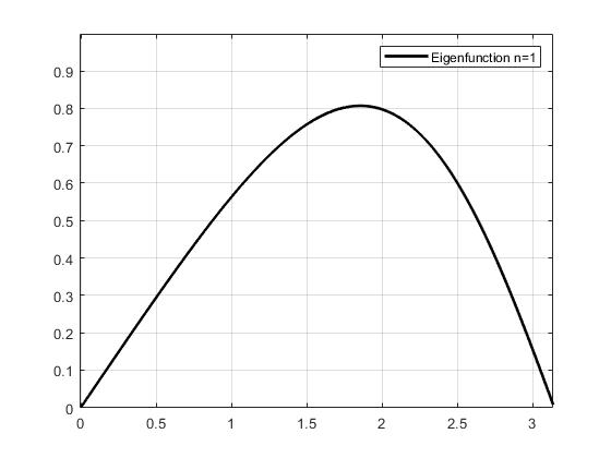
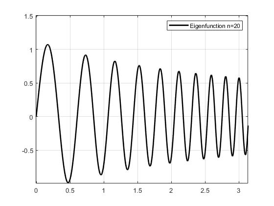
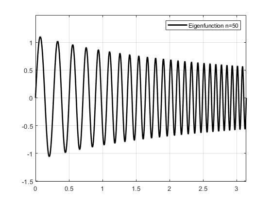
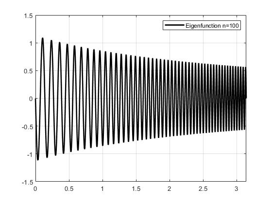
Figure 1: Some eigenfunctions of the Sturm Liouville problem in example 1 with n = 1, 20, 50, 100.

3.2 Example 2:

We consider the Sturm-Liouville eigenvalue problem

$$-\frac{d^{2}y}{dx^{2}}+x^{4}y=\lambda y$$ (12)

with the homogeneous boundary conditions $y(\pm\infty)=0$.

In the study of quantum mechanics, if the potential well $V(x)$ rises monotonically as $x\longrightarrow\pm\infty$, the differential equation

$$\frac{d^{2}y}{dx^{2}}=(V(x)-E)y,$$

describes a particle of energy E confined to a potential well $V(x)$.

The eigenvalue $E$ satisfies

$$\int_{A}^{B}\sqrt{E-V(x)}dx=(n+\frac{1}{2})\pi,$$

where the turning points $A$ and $B$ are the two solutions to the equation $V(x)-E=0$.
The WKB eigenfunctions $y_{n}(x)$ satisfy the formula

$$y_{n}(x)=2\sqrt{\pi}C(\frac{3}{2}S_{0})^{\frac{1}{6}}[V(x)-E]^{-\frac{1}{4}}A_{i}(\frac{3}{2}S_{0})^{\frac{2}{3}},$$

where $S_{0}=\int_{0}^{x}\sqrt{(V(t)-E)}dt$ and $A_{i}$ is the Airy function. ( see  [15])
Thus the eigenvalues of the problem (13) satisfy

$$\lambda_{n}\sim\left[\frac{3\gamma(\frac{3}{4})(n+\frac{1}{2})\sqrt{\pi}}{\gamma(\frac{1}{4})}\right]^{\frac{4}{3}},\quad n\longrightarrow\infty$$

where $\gamma$ is the gamma function.

We use the Chebyshev Collocation Method by discretizing (12) in the interval $[-d,d]$ with the boundary conditions $y(-d)=y(d)=0$:

$$-\frac{d^{2}y}{dx^{2}}+x^{4}y=\lambda y$$ (13)

with the boundary conditions $y(-d)=y(d)=0$.
The collocation approximation to the differential eigenvalue problem (13) is represented by the $(N-1)\times(N-1)$ matrix eigenvalue problem:

$$-D_{N}^{(2)}y+\widetilde{q}y=\lambda y$$ (14)

where $\widetilde{q}=diag(x_{j}^{4})$.

We approximate the solutions of the Sturm-Liouville problem (12) by solving the Matrix eigenvalue problems (13) and (14) using a Chebfun code:

⬇

d = 10;

L = chebop(-d,d);

L . op = @(x,u) - diff(u,2)+(x^4)*u;

L . bc =’dirichlet’;

N = 100;

[V, D] = eigs(L,100);

diag(D)

In table 3, we list the numerical results of this method by computing the first thirty eigenvalues and the relative error between this technique and the WKB approximations by Bender and Orzag  [15]. The numerical results in Table 3 show the high performance of the current technique. Figure 2 shows the numerical computations of relative errors. These results illustrate the high accuracy and efficiency of the algorithms. Figure 3 shows some eigenfunctions of the sturm-liouville problem in example 2 for n = 10, 30, 50 and 100.

Table 3: Computations of the first thirty eigenvalues $\lambda_{n}$ of and the relative error in example 2 with $d=10$

n	$\lambda_{n}$ Current work	$\lambda_{n}^{WKB}$	Relative error $E_{n}=|\frac{\lambda_{n}^{WKB}-\lambda_{n}}{\lambda_{n}^{WKB}}|$
0	1.0603620904849	0.8671453264848	2.22819357E-01
1	3.7996730297979	3.7519199235504	1.27276454E-02
2	7.4556979379858	7.4139882528108	5.62580945E-03
4	11.6447455113774	11.6115253451971	2.86096488E-03
5	16.2618260188517	16.2336146927052	1.73783391E-03
6	21.2383729182367	21.2136533590572	1.16526648E-03
7	26.5284711836832	26.5063355109631	8.35108750E-04
8	32.0985977109688	32.0784641156416	6.27635889E-04
9	37.9230010270330	37.9044718450677	4.88838943E-04
10	43.9811580972898	43.9639483585989	3.91451162E-04
11	50.2562545166843	50.2401523191723	3.20504552E-04
12	56.7342140551754	56.7190570966241	2.67228676E-04
13	63.4030469867205	63.3887079062501	2.26208751E-04
14	70.2523946286162	70.2387714452705	1.93955319E-04
15	77.2732004819871	77.2602101293507	1.68137682E-04
16	84.4574662749449	84.4450400943621	1.47151101E-04
17	91.7980668089950	91.7861473252516	1.29861467E-04
18	99.2886066604955	99.2771452225694	1.15448907E-04
19	106.923307381733	106.912262402219	1.03308819E-04
20	114.696917384982	114.686253003331	9.29874451E-05
21	122.604639001000	122.594324052793	8.41388726E-05
22	130.642068748629	130.632075959854	7.64956746E-05
23	138.805147911395	138.795453260716	6.98484745E-05
24	147.090121257603	147.080703465973	6.40314563E-05
25	155.493502268682	155.484342386656	5.89119257E-05
26	164.012043622866	164.003124693834	5.43826775E-05
27	172.642711962846	172.634018745858	5.03563379E-05
28	181.38266618577	181.374184925625	4.67611207E-05
29	190.229238652464	190.220956887619	4.35376048E-05

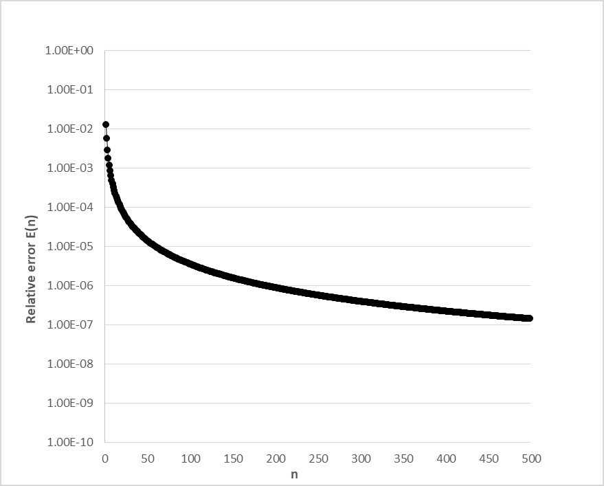
Figure 2: Relative errors E(n) of some high index eigenvalues of the Sturm-Liouville problem in example 2 with $d=10$

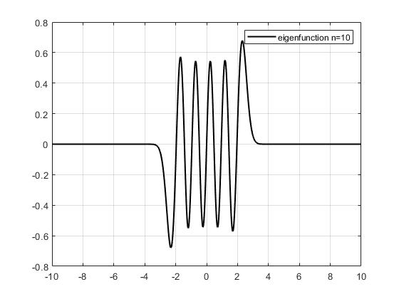
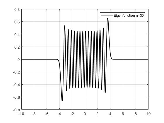
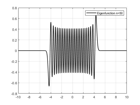
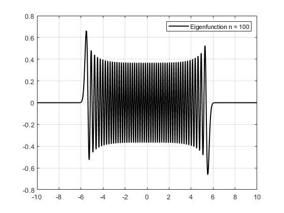
Figure 3: Some eigenfunctions of the Sturm Liouville problem for Example 2 with n = 10, 30, 50, 100 and $d=10$

3.3 Example 3:

We consider the Sturm-Liouville eigenvalue problem

$$-\frac{d^{2}y}{dx^{2}}=\frac{\lambda}{(1+x)^{2}}y$$ (15)

with the boundary conditions $y(0)=y(1)=0$. The exact eigenvalues of the problem (15) satisfy the explicit formula (see  [17]):

$$\lambda_{n}=\frac{1}{4}+(\frac{\pi n}{ln2})^{2},\quad n=1,2,3,...$$

The eigenfunctions $y_{n}(x)$ associated with different eigenvalues $\lambda_{n}$ are given by:

$$y_{n}(x)=\sqrt{1+x}\quad sin(\frac{\pi n}{ln2}ln(1+x)).$$

The collocation approximation of the differential eigenvalue problem (15) is now represented by the $(N-1)\times(N-1)$ matrix eigenvalue problem

$$-D_{N}^{(2)}y=\lambda\widetilde{w}y$$ (16)

where $\widetilde{w}=diag(\frac{1}{(1+x_{j})^{2}})$.
Now, the approximate eigenvalues of the Sturm-Liouville problem (15) are obtained by solving the matrix eigenvalue problem (16) using the Chebyshev Spectral Collocation technique based on Chebfun and Chebop codes.
In table 4, we compute the first thirty eigenvalues and the related absolute error between the numerical calculation and the exact solution

$$E_{n}=\frac{|\lambda_{n}^{exact}-\lambda_{n}|}{|\lambda_{n}^{exact}|}.$$

The eigenvalues obtained are extremely close to the exact eigenvalues. The results show significant improvement in the convergence.
In figure 4, we plot some eigenfunctions in example 3 for $n=1,n=30,n=50$ and $n=80$.

Table 4: Computations of the first thirty eigenvalues $\lambda_{n}$ and the relative error in example 3

n	$\lambda_{n}$ Current work	$\lambda_{n}^{exact}$	Relative error $E_{n}=\frac{|\lambda_{n}^{exact}-\lambda_{n}|}{|\lambda_{n}^{exact}|}$
1	20.79228845522	20.79228845517	2.40469E-12
2	82.4191538209	82.41915382087	3.63913E-13
3	185.13059609701	185.13059609709	4.32157E-13
4	328.92661528358	328.92661528388	9.11961E-13
5	513.8072113806	513.80721137895	3.21132E-12
6	739.77238438806	739.77238439069	3.55512E-12
7	1006.82213430597	1006.82213430587	9.9243E-14
8	1314.95646113432	1314.95646113354	5.93335E-13
9	1664.17536487313	1664.17536487301	7.20502E-14
10	2054.47884552238	2054.47884552193	2.18994E-13
11	2485.86690308208	2485.86690308175	1.32756E-13
12	2958.33953755223	2958.33953755204	6.41739E-14
13	3471.89674893283	3471.89674893313	8.6339E-14
14	4026.53853722387	4026.53853722418	7.70655E-14
15	4622.26490242536	4622.26490242571	7.578E-14
16	5259.0758445373	5259.07584453724	1.13997E-14
17	5936.97136355969	5936.97136355928	6.90036E-14
18	6655.95145949252	6655.95145949275	3.46947E-14
19	7416.0161323358	7416.01613233622	5.65889E-14
20	8217.16538208953	8217.16538208989	4.39108E-14
21	9059.39920875371	9059.3992087539	2.09559E-14
22	9942.71761232833	9942.71761232853	2.00991E-14
23	10867.1205928134	10867.1205928132	1.83894E-14
24	11832.6081502089	11832.6081502087	1.68889E-14
25	12839.1802845148	12839.1802845162	1.09127E-13
26	13886.8369957313	13886.8369957319	4.31718E-14
27	14975.5782838581	14975.5782838589	5.33776E-14
28	16105.4041488954	16105.4041488943	6.82455E-14
29	17276.3145908432	17276.3145908419	7.53159E-14
30	18488.3096097014	18488.3096097008	3.25471E-14

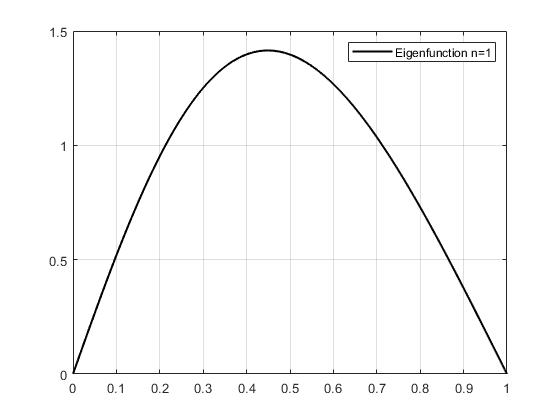
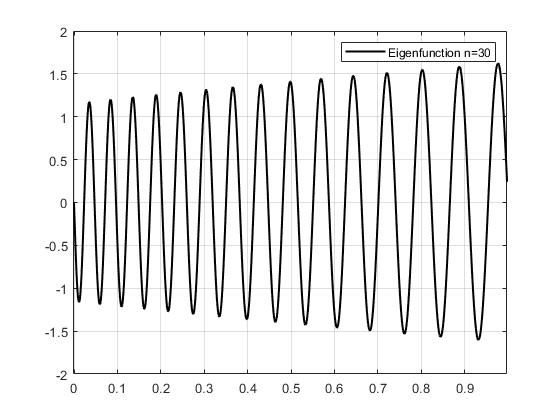
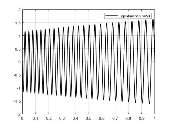
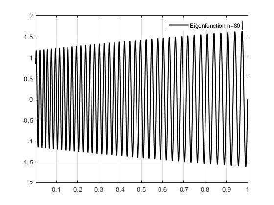
Figure 4: Some eigenfunctions of the Sturm Liouville problem for Example 3 with n = 1, 30, 50, 80.

Conclusion

The numerical computations prove the efficiency of the technique based on the Chebfun and Chebop systems. This technique is unbeatable regarding the accuracy, computation speed, and information it provides on the accuracy of the computational process. Chebfun provides greater flexibility compared to classical spectral methods. However, in the presence of various singularities, the maximum order of approximation can be reached and the Chebfun issues a message that warns about the possible inaccuracy of the computations. The methodology can be used to obtain high-accurate solutions to other Sturm-Liouville problems, generalized differential equations involving higher order derivatives and non-linear partial differential equations in multiple space dimensions.

References

- F. [1994] Siegfried F. Practical quantum mechanics. Classics in Mathematics. (Recherunethoden der Quantentheorie. English).2nd print, 1994.
- George W. Hanson [2002] Alexander B. Yakovlev George W. Hanson. Operator theory for electromagnetics. Springer-Verlag New York, 2002.
- Pryce [1993] J.D Pryce. Numerical solution of sturm–liouville problems. Oxford University Press, New York, 1993.
- Ledoux V. [2005] M.V. Berghe G.V. Ledoux V., Daele. Matslise: a software package for the numerical solution of sturm–liouville and schrödinger problems. ACM Trans. Math. Softw. 31, 532–554, 2005.
- Fulton [1993] Pruess S Fulton, C. Mathematical software for sturm–liouville problems. ACM Trans. Math. Softw.19, 360–376, 1993.
- Bailey [1978] Gordon M. Shampine L. Bailey, P.B. Automatic solution for sturm–liouville problems. ACM Trans.Math. Softw. 4, 193–208, 1978.
- Trefethen [2000] L.N. Trefethen. Spectral methods in matlab. SIAM, 2000.
- Driscoll [2008] Bornemann F. Trefethen L.N. Driscoll, T.A. The chebop system for automatic solution of differential equations. BIT Numerical Mathematics, 2008.
- Aurentz [2017] Trefethen L.N. Aurentz, J.L. Block operators and spectral discretizations. Siam Review. Vol 59.No 2. 423-446, 2017.
- Canuto [1988] M. Y Quarteroni A. ZANG T. A Canuto, C. Hussaini. Spectral methods in fluid dynamics. Springer-Verlag, Berlin, Germany, 1988.
- Fornberg [1996] B. Fornberg. A practical guide to pseudospectral methods. Cambridge University Press, New York, 1996.
- [12] Trefethen L.N. Driscoll T.A., Hale N. Chebfun-numerical computing with functions. http://www.chebfun.org.
- Driscoll T.A. [2014] Trefethen L.N. Driscoll T.A., Hale N. Chebfun guide. Pafnuty publications. Oxford, 2014.
- Weideman [2000] Reddy S.C Weideman, J.A.. A matlab differentiation matrix suite. ACM Trans. Math. Softw. 26, 465–519, 2000.
- Bender and Orszag [1978] C.M. Bender and S.A. Orszag. Advanced mathematical methods for scientists and engineers. McGraw-Hill, New York, 1978.
- E. [1986] Tadmor E. The exponential accuracy of fourier and chebyshev differencing methods. SIAM J. Numer. Anal. 23, 1-10, 1986.
- Akulenko L.D. [2004] Nesterov S.V Akulenko L.D. High-precision methods in eigenvalue problems and their applications. Differential and Integral Equations and Their Applications, Chapman and Hall/CRC, 2004.