Yang-Baxter Hochschild Cohomology

Abstract.

Braided algebras are associative algebras endowed with a Yang-Baxter operator that satisfies certain compatibility conditions involving the multiplication. Along with Hochschild cohomology of algebras, there is also a notion of Yang-Baxter cohomology, which is associated to any Yang-Baxter operator. In this article, we introduce and study a cohomology theory for braided algebras in dimensions 2 and 3, that unifies Hochschild and Yang-Baxter cohomology theories. We show that its second cohomology group classifies infinitesimal deformations of braided algebras. We provide infinite families of examples of braided algebras, including Hopf algebras, tensorized multiple conjugation quandles, and braided Frobenius algebras. Moreover, we derive the obstructions to quadratic deformations, and show that these obstructions lie in the third cohomology group. Relations to Hopf algebra cohomology are also discussed.

1. Introduction

Hochschild homology is defined for associative algebras, and has been studied extensively in deformation theories of algebras [GS]. It corresponds to group homology in discrete case [Brown]. Its 2-dimensional cohomology group, in particular, describes extensions of groups. A counterpart of group homology for self-distributive (SD) structures called racks and quandles has been developed [FR, CJKLS]. The SD structure is related to braiding, and its homology theory has been applied to knot theory [FRS], such as in quandle cohomology theories [CJKLS]. Its 2-dimensional cohomology group describes extensions of racks and quandles as well. Tensor versions of SD structure that correspond to Hochschild homology, and their homology theory, have also been developed [CCES-coalgebra, CCES-adjoint].

The SD structure has been used to construct solutions to the Yang-Baxter equation (YBE) [AZ, CCES-coalgebra]. The YBE has been studied extensively in physics and knot theory as well. In particular in knot theory, solutions to YBE have been employed in the construction of quantum knot invariants. Counterparts of Hochschild homology for the Yang-Baxter equation have been also developed in several ways. A homology theory for set-theoretic YBE, the discrete case, was defined in [CCES1]. Diagrammatic representations have been developed for this theory in [Lebed, PW], through which it was extended to the tensor case. Interpretations of this tensor version do not seem clearly known at this time. A different homology theory for YBE was defined in [Eisermann1, Eisermann] from point of view of the deformation theory. Relations between these two homology theories do not seem to be known. However, a relation between $n$-Lie algebra cohomology, SD cohomology and the Yang-Baxter cohomology of Eisermann has recently been studied in [El-Zap].

Diagrammatics of associative and SD structures have been used effectively in both algebraic and topological context. When a binary operation is represented by a trivalent vertex of a graph, associativity corresponds to the change of tree diagrams called IH-move. As diagrammatic representation of SD operations, crossings of knot diagrams have been employed, that corresponds to the braiding and the YBE.

On the other hand, handlebody-links and surface ribbons (compact orientable surfaces with boundary expressed in knotted ribbon forms) have been represented by spatial trivalent graphs, with sets of moves specified in each context. See [Ishii08, CIST, Matsu]. Thus the idea of using operations that possess both associative and SD (partial) operations has been explored [CIST] in discrete case, and its homology theory has been developed. A tensor version of such structure was proposed in [SZbrfrob], called braided Frobenius algebras, and a construction of such algebras was provided from certain Hopf algebras through quantum heaps.

For both algebraic and knot theoretic perspectives, it naturally arises the question of whether there exists a (co)homology theory for algebras that has both associative and Yang-Baxter (YB) structures, which unifies Hochschild and Yang-Baxter (co)homology theories. Algebras with braiding, called braided algebras, have been defined in [Baez], where a homology theory was also introduced. Homology theories of algebras with braiding present have been studied in contexts different from this paper, for example in [HK, KP]. In this paper we propose a cohomology theory that unifies Yang-Baxter and Hochschild theories. We take an approach from deformation theory, and formulate low dimensional differentials, and show that the cohomology groups play roles in integrability. We point out that our approach differs from [Baez] in that our aim is to obtain a unified theory of Hochschild and YB cohomologies, while in [Baez] the main objective was to encode the braiding operation in the Hochschild homology by replacing the natural switching morphism of the symmetric tensor categories of vector spaces (or modules) by the braiding.

We hereby give a brief overview of the main results of this article. We introduce a chain complex (in low dimensions) that combines Hochschild’s theory of algebra cohomology and Yang-Baxter cohomology, Proposition 3.3. This theory applies to braided algebras, answering in the affirmative the question regarding the existence of a cohomological theory unifying Hochschild cohomology and Yang-Baxter cohomology. We therefore show that the second cohomology group of this cochain complex classifies deformations of braided algebras, which is shown in Theorem 3.8. This result fits in the usual paradigm that the second cohomology group of an algebraic structure with coefficients in itself, controls the deformation theory of the structure. In addition, we derive the obstruction for the existence of quadratic deformations in Theorem 6.5, show that this lies in the third cohomology group in Lemma 6.6 and derive a sufficient condition for the existence of quadratic deformations in Corollary 6.7.

The paper is organized as follows. In Section 2, definitions of braided algebras and examples will be presented, for which the unified cohomology theories of YB and Hochschild can be applied. Yang-Baxter Hochschild homology is defined up to 2-differentials from deformation theory in Section 3. Relations to braided multiplications and Hopf algebra homology are discussed in Sections 4 and 5, respectively. The theory is further extended to 3-differentials using higher deformations in Section 6. Detailed proofs for quadratic deformations are deferred to the appendix.

Throughout the article, following common conventions, we indicate cochain complexes by the letter $C$, cocycles by $Z$ and coboundaries by $B$, all of them with appropriate subscripts and superscripts to indicate the type of complex used, e.g. Hochschild or YB, and the dimension.

2. Braided algebras

In this section we define YI, IY, and braided algebras for which we define Yang-Baxter Hochschild (co)homology, and give examples of such algebras. These are algebras with both multiplication and braiding that satisfy certain compatibility conditions. Throughout this section, and the rest of the article, we assume that all algebras are over a unital commutative ring $\mathbb{k}$, and we use the symbol $\mathbb{1}$ to indicate the identity map. The set ${\rm Hom}_{\mathbb{k}}(V,W)$ of $\mathbb{k}$-module homomorphisms, for $\mathbb{k}$-modules $V$ and $W$, is simply denoted by ${\rm Hom}(V,W)$.

Recall that for an invertible map $R:V\otimes V\rightarrow V\otimes V$ of a ${\mathbb{k}}$-module $V$, the equation

$$(R\otimes{\mathbb{1}})({\mathbb{1}}\otimes R)(R\otimes{\mathbb{1}})=({\mathbb{1}}\otimes R)(R\otimes{\mathbb{1}})({\mathbb{1}}\otimes R)$$

is called the Yang-Baxter equation (YBE), and a solution of it is called a Yang-Baxter (YB) operator.

Definition 2.1.

Let $(V,\mu)$ be a ${\mathbb{k}}$-algebra for a unital ring $\mathbb{k}$, with a YB operator $R:V\otimes V\rightarrow V\otimes V$. We say that $\mu$ and $R$ satisfy the ${\rm YI}$ (resp. ${\rm IY}$) condition if they satisfy

(1) $$(\mu\otimes\mathbb{1})({\mathbb{1}}\otimes R)(R\otimes{\mathbb{1}}) = R\otimes(\mathbb{1}\otimes\mu),$$

(2) $$(\mathbb{1}\otimes\mu)(R\otimes{\mathbb{1}})({\mathbb{1}}\otimes R) = R\otimes(\mu\otimes{\mathbb{1}}),$$

respectively. We call $(V,\mu,R)$ a YI algebra (resp. IY algebra). If $(V,\mu,R)$ satisfies both Equation (1) and Equation (2), we call it a braided algebra.

Definition 2.2.

If $(V_{1},\mu_{1},R_{1})$ and $(V_{2},\mu_{2},R_{2})$ are braided algebras, we say that a linear map $f:V_{1}\rightarrow V_{2}$ is a homomorphism of braided algebras, if $f$ is an algebra homomorphism such that the following diagram commutes

If $f$ admits an inverse that is itself a braided algebra homomorphism, we say that $f$ is a braided isomorphism.

A YB operator and the multiplication $\mu$ are depicted in Figure 1 (A) and (B), respectively, and using these diagrams, Equation (1) and Equation (2) are depicted in (C) and (D), respectively. An array of vertical $n$ edges represents $V^{\otimes n}$, and the diagrams are read from top to bottom, in the direction of homomorphisms. A crossing in (A) represents a YB operator $R:V^{\otimes 2}\rightarrow V^{\otimes 2}$, and a trivalent vertex in (B) represents a multiplication $\mu:V^{\otimes 2}\rightarrow V$.

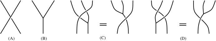
Figure 1.

2.1. Braided algebras from tensorized multiple conjugation quandles

We show that tensorization of multiple conjugation quandles (MCQs) [CIST] produces braided algebras.

First, recall a quandle [Joyce82, Matveev82], is a non-empty set $X$ with a binary operation $*:X\times X\to X$ satisfying the following axioms.

• For any $a\in X$, we have $a*a=a$.

• For any $a\in X$, the map $S_{a}:X\to X$ defined by $S_{a}(x)=x*a$ is a bijection.

• For any $a,b,c\in X$, we have $(a*b)*c=(a*c)*(b*c)$.

A rack is a set with an operation that satisfies (2) and (3).

Definition 2.3 ([Ishii08]).

A multiple conjugation quandle (MCQ) $X$ is the disjoint union of groups $G_{\lambda}$, where $\lambda$ is an element of an index set $\Lambda$, with a binary operation $*:X\times X\to X$ satisfying the following axioms.

• For any $a,b\in G_{\lambda}$, we have $a*b=b^{-1}ab$.

• For any $x\in X$, $a,b\in G_{\lambda}$, we have $x*e_{\lambda}=x$ and $x*(ab)=(x*a)*b$, where $e_{\lambda}$ is the identity element of $G_{\lambda}$.

• For any $x,y,z\in X$, we have $(x*y)*z=(x*z)*(y*z)$ (self-distributivity).

• For any $x\in X$, $a,b\in G_{\lambda}$, we have $(ab)*x=(a*x)(b*x)$ in some group $G_{\mu}$.

We call the group $G_{\lambda}$ a component of the MCQ. An MCQ is a type of quandle that can be decomposed as a union of groups, and the quandle operation in each component is given by conjugation. Moreover, there are compatibilities, (2) and (4), between the group and quandle operations. In [Ishii08], concrete examples of MCQs are presented.

Example 2.4.

Let $X=\sqcup_{\lambda\in\Lambda}G_{\lambda}$ be an MCQ with a quandle operation $*$. Let ${\mathbb{k}}[X]$ be the free ${\mathbb{k}}$-module generated by $X$. Define a multiplication $\mu:{\mathbb{k}}[X]\otimes{\mathbb{k}}[X]\rightarrow{\mathbb{k}}[X]$ on generators by $\mu(x\otimes y):=xy$ if $x,y\in G_{\lambda}$ for some $\lambda\in\Lambda$, and $\mu(x\otimes y):=0$ otherwise, and extended linearly. Define $R:{\mathbb{k}}[X]\otimes{\mathbb{k}}[X]\rightarrow{\mathbb{k}}[X]\otimes{\mathbb{k}}[X]$ on generators $x,y\in X$ by $R(x\otimes y):=y\otimes(x*y)$ and extended linearly. Then ${\mathbb{k}}[X]$ is a braided algebra, as we now proceed to show. If two of $x,y,z\in X$ belong to distinct $G_{\lambda}$’s, then the triple product is $0$, and if all belong to the same $G_{\lambda}$ then it is associative, hence $\mu$ is associative. Equations (1) and (2), respectively, follow from the conditions $(ab)*x=(a*x)(b*x)$ and $x*(ab)=(x*a)*b$ for any $x\in X$, $a,b\in G_{\lambda}$ on generators, and if $a,b$ belong to distinct $G_{\lambda}$ then the values are $0$ for both sides of the equations, hence ${\mathbb{k}}[X]$ is a YI and IY algebra.

Another type of discrete racks with partial multiplication is a rack constructed from a group heap. The following construction is found in [SZframedlinks, SZsfceribbon]. Let $G$ be a group, and consider the ternary operation on $G$ defined by $T(x,y,z):=xy^{-1}z$. A group $G$ with this operation is called a heap, and $T$ satisfies the ternary self-distributive property,

$$T(T(x,y,z),u,v)=T(T(x,u,v),T(y,u,v),T(z,u,v)).$$

By this property, it follows that the binary operation defined on $X=G\times G$ by $(x,y)*(u,v):=(T(x,u,v),T(y,u,v))=(xu^{-1}v,yu^{-1}v)$ is self-distributive. Property (2) above is also satisfied, and $(X,*)$ is a rack. An argument similar to the one in Example 2.4 gives the following.

Example 2.5.

Let $G$ be a group heap, and let $(X,*)$, $X=G\times G$, be a rack defined above. Let ${\mathbb{k}}[X]$ be the free abelian group generated by $X$. Define a multiplication $\mu:{\mathbb{k}}[X]\otimes{\mathbb{k}}[X]\rightarrow{\mathbb{k}}[X]$ on generators $(x,y),(u,v)\in X$ by $\mu((x,y)\otimes(u,v)):=(x,v)$ if $y=u$, and $\mu(x\otimes y):=0$ otherwise, and extended linearly. Define $R:{\mathbb{k}}[X]\otimes{\mathbb{k}}[X]\rightarrow{\mathbb{k}}[X]\otimes{\mathbb{k}}[X]$ on generators $(x,y),(u,v)\in X$ by

$$R((x,y)\otimes(u,v)):=(u,v)\otimes[(x,y)*(u,v)]=(u,v)\otimes(xu^{-1},yu^{-1}v)$$

and extended linearly. Then ${\mathbb{k}}[X]$ is a braided algebra.

2.2. Brief overview of Hopf algebras

Before giving the constructions that constitute the main examples of braided algebras considered in this article, we briefly recall the notion of Hopf algebra. We also recall some of the properties of Hopf algebras needed to apply the results of [SZbrfrob], which we follow in the exposition of this subsection.

A Hopf algebra $(X,\mu,\eta,\Delta,\epsilon,S)$ (a module over a unital ring $\mathbb{k}$, multiplication, unit, comultiplication, counit, antipode, respectively), is defined as follows. First, recall that a bialgebra $X$ is a module endowed with a multiplication $\mu:X\otimes X\rightarrow X$ with unit $\eta$ and a comultiplication $\Delta:X\rightarrow X\otimes X$ with counit $\epsilon$ such that the compatibility conditions

$$\Delta\circ\mu=(\mu\otimes\mu)\circ({\mathbb{1}}\otimes\tau\otimes{\mathbb{1}})\circ(\Delta\otimes\Delta),$$

$$\epsilon\mu=\epsilon\otimes\epsilon,\ \ \ \Delta\eta=\eta\otimes\eta,\ \ \ \epsilon\eta=\mathbb{1}$$

hold, where $\tau$ denotes the transposition $\tau(x\otimes y)=y\otimes x$ for simple tensors. A Hopf algebra is a bialgebra endowed with a map $S:X\rightarrow X$, called antipode, satisfying the equations

$$\mu\circ(\mathbb{1}\otimes S)\circ\Delta=\eta\circ\epsilon=\mu\circ(S\otimes\mathbb{1})\circ\Delta,$$

called the antipode condition. Antipodes are antihomomorphisms.

Any Hopf algebra satisfies the equality $S\circ\mu\circ\tau=\mu\circ(S\otimes S)$. A Hopf algebra is called involutory if $S^{2}={\mathbb{1}}$, the identity. It is known, [Kas] Theorem III.3.4, that if a Hopf algebra is commutative or cocommutative it follows that it is also involutory.

For the comultiplication, we use Sweedler’s notation $\Delta(x)=x^{(1)}\otimes x^{(2)}$ suppressing the summation. Further, we use

$$(\Delta\otimes{\mathbb{1}})\Delta(x)=(x^{(11)}\otimes x^{(12)})\otimes x^{(2)}\quad{\rm and}\quad({\mathbb{1}}\otimes\Delta)\Delta(x)=x^{(1)}\otimes(x^{(21)}\otimes x^{(22)}),$$

both of which are also written as $x^{(1)}\otimes x^{(2)}\otimes x^{(3)}$ from the coassociativity.

A left integral of $X$ is an element $\lambda\in X$ such that $x\lambda=\epsilon(x)\lambda$ for all $x\in X$, where juxtaposition of elements denotes multiplication applied. Right integrals and (two-sided) integrals, are defined similarly. The existence of integrals is a fundamental tool to endow a Hopf algebra with a Frobenius structure. It is known that the set of integrals of a free finite dimensional Hopf algebra over a PID admits a one dimensional space of integrals, see [LS]. More generally, a finitely generated projective Hopf algebra over a ring admits a left integral space of rank one [Par]. Observe that when a Hopf algebra is (co)commutative, it follows that a left integral is also a right integral.

2.3. Braided algebras from Hopf algebras

We now describe an important class of braided algebras related to MCQs derived from Hopf algebras. First, recall [EZ] that given a Hopf algebra $H$, one has a Yang-Baxter operator $R_{H}$ associated to it defined through the left adjoint action of $H$ on itself, which is a generalization of the notion of conjugation in a group:

$$R_{H}:x\otimes y\mapsto y^{(1)}\otimes S(y^{(2)})xy^{(3)},$$

where juxtaposition here indicates multiplication in $H$, and we have employed Sweedler’s notation. Observe that when $H$ is the group algebra of a group $G$, where $S(g)=g^{-1}$ for all $g\in G$, then the YB operator $R_{H}$ coincides with the YB operator obtained by linearizing the group $G$ and endowing the corresponding group algebra with the standard Hopf algebra structure, where the comultiplication is diagonal and the antipode is induced by taking inverses in $G$.

Lemma 2.6.

Let $(H,\mu,\Delta,\eta,\epsilon.S)$ be a Hopf algebra and let $R_{H}$ denote the YB operator defined above. Then $(H,\mu,R_{H})$ is a braided algebra.

Proof.

We show that Equation (2) holds on simple tensors. A similar procedure can be performed for Equation (1). For the left hand side of Equation (2) we have

$$(\mu\otimes\mathbb{1})(\mathbb{1}\otimes R_{H})(R_{H}\otimes\mathbb{1})(x\otimes y\otimes z) = (\mu\otimes\mathbb{1})(\mathbb{1}\otimes R_{H})(y^{(1)})\otimes S(y^{(2)})xy^{(3)}\otimes z$$

$$= (\mu\otimes\mathbb{1})(y^{(1)})\otimes z^{(3)}\otimes S(z^{(2)})S(y^{(2)})xy^{(3)}z^{(3)}$$

$$= y^{(1)}z^{(1)}\otimes S(z^{(2)})S(y^{(2)})xy^{(3)}z^{(3)}$$

while for the right hand side of Equation (2) we have

$$R_{H}(\mathbb{1}\otimes\mu)(x\otimes y\otimes z) = R_{H}(x\otimes yz)$$

$$= (yz)^{(1)}\otimes S((yz)^{(2)})x(yz)^{(3)},$$

The two expressions are easily seen to coincide, using the fact that $\mu$ and $\Delta$ satisfy the Hopf algebra axioms, and the fact that $S$ is a antihomomorphism of algebras. ∎

2.4. Braided Frobenius algebras from (co-)commutative Hopf algebras

In [SZbrfrob], braided Frobenius algebras (i.e. a class of braided algebras) were constructed from commutative and cocommutative Hopf algebras. This is a Hopf algebra version of the heap construction described above. We briefly review the construction.

Let $(X,m,\eta,\Delta,\epsilon,S)$ be a commutative and cocommutative Hopf algebra, where the listed data are multiplication, unit, comultiplication, counit, and the antipode, respectively. Then $V=X\otimes X$ was given a braided Frobenius algebra structure, in particular braided algebra, with the following YB operator and the multiplication.

The YB operator is defined as follows. First, introduce $T:X\otimes X\otimes X\rightarrow X$ by letting $T(x\otimes y\otimes z)$ be defined on simple tensors as $T(x\otimes y\otimes z):=xS(y)z$, where juxtaposition indicates, as before, Hopf algebra multiplication $m$. Note that this corresponds to the operation $xy^{-1}z$ for group heaps. Then the map $R:V^{\otimes 2}\rightarrow V^{\otimes 2}$ is defined for simple tensors by

$$R((x\otimes y)\otimes(z\otimes w)):=(z^{(1)}\otimes w^{(1)})\otimes T(x\otimes z^{(2)}\otimes w^{(2)})\otimes T(y\otimes z^{(3)}\otimes w^{(3)}).$$

It was shown that this $R$ indeed satisfies the YBE.

The multiplication $\mu$ on $V\otimes V$ was defined as follows. There exists an integral $\lambda:V\rightarrow{\mathbb{k}}$ in a Hopf algebra in question, and the map $\cup:V\otimes V\rightarrow{\mathbb{k}}$ is defined by $\cup:=\lambda m({\mathbb{1}}\otimes S)$. Then the multiplication is defined by $\mu={\mathbb{1}}\otimes\cup\otimes{\mathbb{1}}$. It was shown in [SZbrfrob] that these $R$ and multiplication give rise to braided algebras.

In summary, in this section, definitions of YI condition (Equation (1)), IY condition (Equation (2)), braided algebras, and concrete examples of such structures have been presented. In the following sections we propose (co)homology theories for these structures that unify both Hochschild and Yang-Baxter homology theories.

3. Yang-Baxter Hochschild cohomology up to dimension 3 and deformations

In this section we propose low dimensional Yang-Baxter Hochschild cohomology from point of view of deformation theory, and prove the classification theorem for deformations up to equivalence. The main result of this section is Theorem 3.8, which motivates the definition of Yang-Baxter Hochschild chomology of this article, as the algebraic tool controlling infinitesimal deformations.

3.1. Hochschild cohomology

In this section we briefly review deformation theoretic aspects of low dimensional Hochschild cohomology for the simplest case. Let $(V,\mu)$ be an associative algebra over ${\mathbb{k}}$. All homomorphism groups, ${\rm Hom}_{\mathbb{k}}$ over ${\mathbb{k}}$, are denoted by ${\rm Hom}$ for simplicity. The cochain groups of Hochschild cohomology are defined to be $C_{\rm H}^{n}(V,V)={\rm Hom}(V^{\otimes n},V)$ for $n\geq 0$.

The differential in degree zero is given by

$$\delta^{0}_{\rm H}(s)=\mu(\mathbb{1}\otimes s)-\mu(s\otimes\mathbb{1}),$$

for $s:\mathbb{k}\rightarrow V$.

The differentials $\delta^{1}_{\rm H}$ and $\delta^{2}_{\rm H}$ are defined for $f\in C_{\rm H}^{1}(V,V)$ and $\psi\in C_{\rm H}^{2}(V,V)$ by

$$\delta^{1}_{\rm H}(f) = \mu(f\otimes{\mathbb{1}})+\mu({\mathbb{1}}\otimes f)-f\mu,$$

$$\delta^{2}_{\rm H}(\psi) = \mu(\psi\otimes{\mathbb{1}})+\psi(\mu\otimes{\mathbb{1}})-\mu({\mathbb{1}}\otimes\psi)-\psi({\mathbb{1}}\otimes\mu).$$

We note that usual differential for Hochschild cohomology has the opposite sign of $\delta^{2}_{\rm H}$ written above. This convention is for convenience of computations of deformations and diagrams that follow, and also similar to [CCES-coalgebra]. This does not have any implication in the results that follow.

Diagrammatic presentations of the differentials are depicted in Figures 2 and 3. An array of vertical $n$ edges represents $V^{\otimes n}$, and a circle on an edge represents $f:V\rightarrow V$. The diagrams are read from top to bottom, in the direction of a homomorphism. A trivalent vertex represents a multiplication $\mu:V^{\otimes 2}\rightarrow V$, and a circled trivalent vertex represent $\psi$.

Figure 2.

Figure 3.

Let $(V,\mu)$ be an algebra over $\mathbb{k}$. We say that an algebra $(V^{\prime},\mu^{\prime})$ over the power series $\mathbb{k}[[\hbar]]$ is a deformation of $V$ if the quotient algebra $(V^{\prime}/(\hbar)V^{\prime},\mu^{\prime})$ coincides with $(V,\mu)$.

Let $(V,\mu)$ be an associative algebra, $\tilde{V}=V\otimes_{\mathbb{k}}{\mathbb{k}}[[\hbar]]/(\hbar^{2})\cong V\oplus\hbar V$, and $\psi\in Z^{2}_{\rm H}(V,V)$. Then, setting $\tilde{\mu}=\mu+\hbar\psi$, $(\tilde{V},\tilde{\mu})$ is an algebra if and only if the equations $\delta^{2}_{\rm H}(\psi)=0$ hold. This is seen by computing the associativity in $\tilde{V}$,

$$\tilde{\mu}(\tilde{\mu}\otimes{\mathbb{1}}) = (\mu+\hbar\psi)((\mu+\hbar\psi)\otimes{\mathbb{1}})$$

$$= \mu(\mu\otimes{\mathbb{1}})+\hbar[\mu(\psi\otimes{\mathbb{1}})+\psi(\mu\otimes{\mathbb{1}})],$$

$$\tilde{\mu}({\mathbb{1}}\otimes\tilde{\mu}) = (\mu+\hbar\psi)({\mathbb{1}}\otimes(\mu+\hbar\psi)$$

$$= \mu({\mathbb{1}}\otimes\mu)+\hbar[\mu({\mathbb{1}}\otimes\psi)+\psi({\mathbb{1}}\otimes\mu)].$$

In this case, we also have $\tilde{\mu}\equiv_{(\hbar)}\mu$, meaning that $\tilde{\mu}$ coincides with $\mu$ modulo $(\hbar)$, and we say that $(\tilde{V},\tilde{\mu})$ is an infinitesimal deformation of $(V,\mu)$. Thus we say that the primary obstruction to the infinitesimal deformation vanishes if and only if $\delta^{2}_{\rm H}(\psi)=0$.

3.2. Yang-Baxter cohomology up to dimension 3

In this section we define Yang-Baxter (deformation) cohomology. Let $(V,R)$ be a ${\mathbb{k}}$-module with the YB operator $R:V^{\otimes 2}\rightarrow V^{\otimes 2}$. The cochain groups are defined by $C^{0}_{\rm YB}(V,V)=0$ and $C^{n}_{\rm YB}(V,V)={\rm Hom}(V^{\otimes n},V^{\otimes n})$ for $n>0$. We define the differentials for $f\in C^{1}_{\rm YB}(V,V)$ and $\phi\in C^{2}_{\rm YB}(V,V)$ by

$$\delta^{1}_{\rm YB}(f) = R(f\otimes{\mathbb{1}})+R({\mathbb{1}}\otimes f)-(f\otimes{\mathbb{1}})R-({\mathbb{1}}\otimes f)R,$$

$$\delta^{2}_{\rm YB}(\phi) = (R\otimes{\mathbb{1}})({\mathbb{1}}\otimes R)(\phi\otimes{\mathbb{1}})+(R\otimes{\mathbb{1}})({\mathbb{1}}\otimes\phi)(R\otimes{\mathbb{1}})+(\phi\otimes{\mathbb{1}})({\mathbb{1}}\otimes R)(R\otimes{\mathbb{1}})$$

$$-({\mathbb{1}}\otimes R)(R\otimes{\mathbb{1}})({\mathbb{1}}\otimes\phi)-({\mathbb{1}}\otimes R)(\phi\otimes{\mathbb{1}})({\mathbb{1}}\otimes R)-({\mathbb{1}}\otimes\phi)(R\otimes{\mathbb{1}})({\mathbb{1}}\otimes R).$$

The differentials are depicted in Figures 4 and 5. The cochains $f$ and $\phi$ are represented by circles on an edge and a crossing, respectively.

Figure 4.

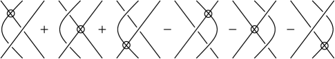
Figure 5.

Lemma 3.1.

The sequence $C^{0}_{\rm YB}(V,V)\rightarrow C^{1}_{\rm YB}(V,V)\stackrel{{\scriptstyle\delta^{1}_{\rm YB}}}{{\longrightarrow}}C^{2}_{\rm YB}(V,V)\stackrel{{\scriptstyle\delta^{2}_{\rm YB}}}{{\longrightarrow}}C^{2}_{\rm YB}(V,V)$ defines a cochain complex.

Proof.

Let $f$ be a YB $1$-cochain. Then, the lemma is proved by showing that $\delta^{2}_{\rm YB}(\phi)=0$ when $\phi=\delta^{1}_{\rm YB}(f)$. Diagrammatically, when $\delta^{1}_{\rm YB}(f)$ is substituted in $\phi$, the circles crossing representing $\phi$ are replaced by four terms with circles placed at the four edges adjacent to the crossing. For example, the first term of $\delta^{2}_{\rm YB}(\phi)$ is shown in Figure 6 left top, and the replacement representing the substitution is depicted in the right of the top row. Similar diagrams are shown in the middle row for the second term of $\delta^{2}_{\rm YB}(\phi)$. One sees that the terms labeled (B) and (C) in the top and the middle row cancel with opposite signs. This cancelation principle is explained by the fact that each edge is shared by two crossings. In Figure 6, the terms labeled (A) in the top row and (D) in the bottom row have the circles for $f$ placed at the end edge (top). They are canceled by opposite signs after applying the YBE (in diagrammatic form). Hence in both cases (the circle placed inside or end edges), two terms cancel with opposite signs, and we obtain $\delta^{2}_{\rm YB}(\phi)=0$. ∎

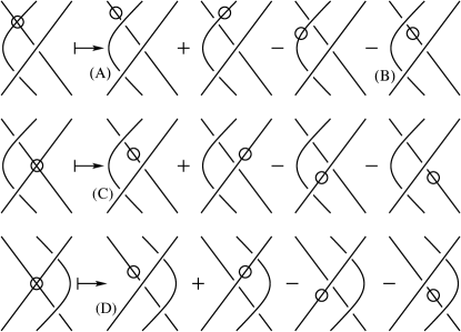
Figure 6.

Remark 3.2.

Deformation cohomology theory was developed in [Eisermann] for all dimensions. The cochains in [Eisermann] differ from ours by compositions of YB operators. For example, the 2-cochain $c^{\prime}$ in [Eisermann] is written as $Rc$ for our 2-cochain $c$. We adopt our definition and diagrammatics along the line of [CCES-coalgebra, CCES-adjoint] for the purpose of unifying Yang-Baxter cohomology with algebra cohomology.

3.3. Yang-Baxter Hochschild cohomology up to dimension $3$

Let $V$ be a braided algebra with coefficient unital ring ${\mathbb{k}}$. We define the cochain groups for a braided algebra $V$ with coefficients in itself up to degree $3$ as follows. We set $C_{\rm YBH}^{0}(V,V)=0$, and $C^{n,k}_{\rm YBH}(V,V)={\rm Hom}(V^{\otimes n},V^{\otimes k})$ for $n,k>0$. We also use different subscripts

$$C^{n,k}_{\rm YI}(V,V)={\rm Hom}(V^{\otimes n},V^{\otimes k})=C^{n,k}_{\rm IY}(V,V)$$

to distinguish different isomorphic direct summands. Define

$$C_{\rm YBH}^{1}(V,V) = C^{1,1}_{\rm YBH}(V,V)={\rm Hom}(V,V),$$

$$C^{2}_{\rm YBH}(V,V) = C^{2,2}_{\rm YBH}(V,V)\oplus C^{2,1}_{\rm YBH}(V,V),\quad{\rm and}$$

$$C^{3}_{\rm YBH}(V,V) = C^{3,3}_{\rm YBH}(V,V)\oplus C^{3,2}_{\rm YI}(V,V)\oplus C^{3,2}_{\rm IY}(V,V)\oplus C^{3,1}_{\rm YBH}(V,V).$$

We define differentials as follows. We set $\delta^{1}_{\rm YBH}$ to be the direct sum $\delta^{1}_{\rm YB}\oplus\delta^{1}_{\rm H}$.

The second differential $\delta^{2}_{\rm YBH}$ is defined to be the direct sum of four terms $\delta^{2}_{\rm YB}\oplus\delta^{2}_{\rm YI}\oplus\delta^{2}_{\rm IY}\oplus\delta^{2}_{\rm H}$ where $\delta^{2}_{\rm YB}$ and $\delta^{2}_{\rm H}$ map in the first ($C^{3,3}_{\rm YBH}(V,V)={\rm Hom}(V^{\otimes 3},V^{\otimes 3})$) and last $(C^{3,1}_{\rm YBH}(V,V)={\rm Hom}(V^{\otimes 3},V)$) copies of $C^{3}_{\rm YBH}(V,V)$, respectively, while $\delta^{2}_{\rm YI}$ and $\delta^{2}_{\rm IY}$ map to the middle two factors $C^{3,2}_{\rm YI}(V,V)$ and $C^{3,2}_{\rm IY}(V,V)$, respectively. Each differential is defined as follows.

$$\delta^{2}_{\rm YI}(\phi\oplus\psi) = (\mathbb{1}\otimes\psi)(R\otimes\mathbb{1})(\mathbb{1}\otimes R)+(\mathbb{1}\otimes\mu)(\phi\otimes\mathbb{1})(\mathbb{1}\otimes R)$$

$$+(\mathbb{1}\otimes\mu)(R\otimes\mathbb{1})(\mathbb{1}\otimes\phi)-R(\psi\otimes\mathbb{1})-\phi(\mu\otimes\mathbb{1}).$$

$$\delta^{2}_{\rm IY}(\phi\oplus\psi) = (\psi\otimes\mathbb{1})(\mathbb{1}\otimes R)(R\otimes\mathbb{1})+(\mu\otimes\mathbb{1})(\mathbb{1}\otimes\phi)(R\otimes\mathbb{1})$$

$$+(\mu\otimes\mathbb{1})(\mathbb{1}\otimes R)(\phi\otimes\mathbb{1})-R(\mathbb{1}\otimes\psi)-\phi(\mathbb{1}\otimes\mu).$$

The differential $\delta^{2}_{\rm IY}(\phi\oplus\psi)$ is represented diagrammatically in Figure 7, where 2-cochains $\phi\in C^{2,2}_{\rm YBH}(V,V)$ and $\psi\in C^{3,1}_{\rm YBH}(V,V)$ are represented by 4-valent (resp. 3-valent) vertices with circles. The YI and IY components of the cochain complex above are included to enforce the coherence axioms between deformed algebra structure, and deformed YB operator. In other words, they ensure that YBH $2$-cocycles satisfy Equation (1) and Equation (2), respectively.

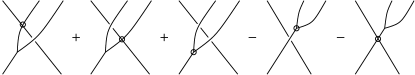
Figure 7.

Proposition 3.3.

The sequence

$$C_{\rm YBH}^{0}(V,V)\rightarrow C_{\rm YBH}^{1}(V,V)\stackrel{{\scriptstyle\delta^{1}_{\rm YBH}}}{{\longrightarrow}}C_{\rm YBH}^{2}(V,V)\stackrel{{\scriptstyle\delta^{2}_{\rm YBH}}}{{\longrightarrow}}C_{\rm YBH}^{3}(V,V)$$

defines a cochain complex.

Proof.

Let $f$ be a YBH $1$-cochain. Setting $\psi=\delta^{1}_{\rm H}(f)$ and $\phi=\delta^{1}_{\rm YB}(f)$, we show that $\delta^{2}_{i}(\phi\oplus\psi)=0$ for $i={\rm YI},{\rm IY}$. The procedure showing that $\delta^{2}_{\rm YI}(\phi\oplus\psi)=0$ is depicted in Figures 8 and 9, and similar to the proof of Lemma 3.1. In the right column of Figure 8, the positive terms of $\delta^{2}_{\rm IY}(\phi\oplus\psi)$ depicted in Figure 7 are shown. Circled vertices represent $\psi$ (3-valent vertices) and $\phi$ (4-valent ones). Under the assumption $\psi=\delta^{1}_{\rm H}(f)$ and $\phi=\delta^{1}_{\rm YB}(f)$, each vertex is replaced by a linear combination of the diagrams with circles (representing $f$) on edges, according to the definition of $\delta^{1}(f)$ (Figure 2). Such linear combinations for each term in the left column of Figure 8 are depicted in the right column of the figure. Thus $\psi=\delta^{1}_{\rm H}(f)$ and $\phi=\delta^{1}_{\rm YB}(f)$ is represented by replacing the positive terms in Figure 7 by the right columns in Figure 8. The negative terms are similarly replaced by the right columns in Figure 9. With signs one sees that all terms cancel, indicating $\delta^{2}_{\rm IY}(\phi\oplus\psi)=0$. The case $\delta^{2}_{\rm YI}(\phi\oplus\psi)=0$ is similar. The other differentials for YBE and Hochschild are similar as well. ∎

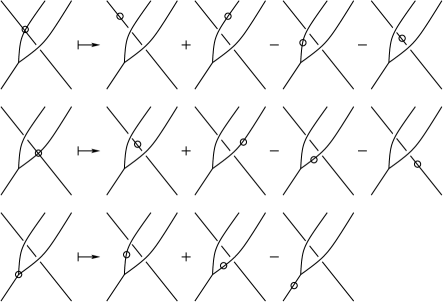
Figure 8.

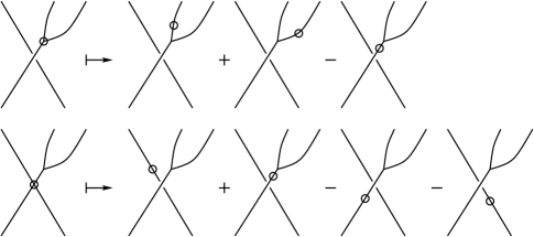
Figure 9.

3.4. Infinitesimal deformations of braided algebras

Let $(V,\mu,R)$ be a braided algebra over $\mathbb{k}$. Let us consider the power series ring $\mathbb{k}[[\hbar]]$ over the formal variable $\hbar$, and let $(\hbar)$ denote the ideal of $\mathbb{k}[[\hbar]]$ generated by $\hbar$.

Definition 3.4.

Let $(V,\mu,R)$ be a braided algebra over ${\mathbb{k}}$. Extend $\mu$ and $R$ to $\tilde{V}=V\otimes_{\mathbb{k}}{\mathbb{k}}[[\hbar]]/(\hbar^{2})\cong V\oplus\hbar V$ by linearly extending on $\hbar V$ and use the same notation $\mu$ and $R$ on $\tilde{V}$. We say that $(\tilde{V},\tilde{\mu},\tilde{R})$ is an infinitesimal deformation of $(V,\mu,R)$ if ${\rm Im}(\tilde{\mu}-\mu)\subset\hbar V$ and ${\rm Im}(\tilde{R}-R)\subset\hbar(V\otimes V)$. Similar definitions hold for YI algebras and IY algebras.

Let $(V,\mu,R)$ be a braided algebra, and let $(\tilde{V},\tilde{\mu},\tilde{R})$ and $(\hat{V},\hat{\mu},\hat{R})$ be two infinitesimal deformations of $V$. Let $\tilde{f}:\tilde{V}\rightarrow\hat{V}$ be a homomorphism of braided algebras (Definition 2.2). Then, we say that $f$ is a homomorphism of infinitesimal deformations if $\tilde{f}|_{V}:V\rightarrow V$ is the identity map $\mathbb{1}_{V}$. A homomorphism of infinitesimal deformations that is invertible through a homomorphism of infinitesimal deformations is said to be an isomorphism of infinitesimal deformations.

If $(\tilde{V},\tilde{\mu},\tilde{R})$ is an infinitesimal deformation of $(V,\mu,R)$, then we can write

$$\tilde{\mu} = \mu+\hbar\psi$$

$$\tilde{R} = R+\hbar\phi,$$

where $\psi:V\otimes V\rightarrow V$ and $\phi:V\otimes V\rightarrow V\otimes V$.

Remark 3.5.

Recall that in order for $\tilde{\mu}$ to satisfy the associativity condition, $\psi$ needs to be a Hochschild $2$-cocycle, while $\tilde{R}$ is a YB operator if and only if $\phi$ is a YB $2$-cocycle.

Since the latter fact is not found as commonly in the literature as the former, we give a brief proof of it. See also [Eisermann, Eisermann1]. We set $\phi_{0}:=R$ and $\phi_{1}:=\phi$ for notational convenience. The YBE for $\tilde{R}$ then gives us for the left hand side (modulo terms of quadratic order or higher in $\hbar$)

$$(\tilde{R}\otimes\mathbb{1})(\mathbb{1}\otimes\tilde{R})(\tilde{R}\otimes\mathbb{1}) = (\phi_{0}\otimes\mathbb{1})(\mathbb{1}\otimes\phi_{0})(\phi_{0}\otimes\mathbb{1})+\hbar\sum_{i+j+k=1}(\phi_{i}\otimes\mathbb{1})(\mathbb{1}\otimes\phi_{j})(\phi_{k}\otimes\mathbb{1}).$$

Similarly, for the right hand side of the YBE, modulo terms at least quadratic in $\hbar$ we have

$$(\mathbb{1}\otimes\tilde{R})(\tilde{R}\otimes\mathbb{1})(\mathbb{1}\otimes\tilde{R}) = (\mathbb{1}\otimes\phi_{0})(\phi_{0}\otimes\mathbb{1})(\mathbb{1}\otimes\phi_{0})+\hbar\sum_{i+j+k=1}(\mathbb{1}\otimes\phi_{i})(\phi_{j}\otimes\mathbb{1})(\mathbb{1}\otimes\phi_{k}).$$

Therefore, the YBE holds for $\tilde{R}$ if and only if

$$0 = \sum_{i+j+k=1}(\phi_{i}\otimes\mathbb{1})(\mathbb{1}\otimes\phi_{j})(\phi_{k}\otimes\mathbb{1})-\sum_{i+j+k=1}(\mathbb{1}\otimes\phi_{i})(\phi_{j}\otimes\mathbb{1})(\mathbb{1}\otimes\phi_{k})$$

$$= (\phi_{1}\otimes\mathbb{1})(\mathbb{1}\otimes\phi_{0})(\phi_{0}\otimes\mathbb{1})+(\phi_{0}\otimes\mathbb{1})(\mathbb{1}\otimes\phi_{1})(\phi_{0}\otimes\mathbb{1})+(\phi_{0}\otimes\mathbb{1})(\mathbb{1}\otimes\phi_{0})(\phi_{1}\otimes\mathbb{1})$$

$$-(\mathbb{1}\otimes\phi_{1})(\phi_{0}\otimes\mathbb{1})(\mathbb{1}\otimes\phi_{0})-(\mathbb{1}\otimes\phi_{0})(\phi_{1}\otimes\mathbb{1})(\mathbb{1}\otimes\phi_{0})-(\mathbb{1}\otimes\phi_{0})(\phi_{0}\otimes\mathbb{1})(\mathbb{1}\otimes\phi_{1})$$

which is exactly the $2$-cocycle condition for YB cohomology.

Lemma 3.6.

Let $(V,\mu,R)$ be a braided algebra, and let $\psi$ and $\phi$ denote an algebra $2$-cocycle and a YB $2$-cocycle, respectively. Then, setting $\tilde{\mu}=\mu+\hbar\psi$ and $\tilde{R}=R+\hbar\phi$, $(\tilde{V},\tilde{\mu},\tilde{R})$ is an infinitesimal braided algebra deformation of $(V,\mu,R)$ if and only if the equations $\delta^{2}_{\rm YBH}(\phi\oplus\psi)=0$ hold.

Proof.

Since $\psi$ and $\phi$ are algebra and YB $2$-cocycles, respectively, it follows that $\tilde{\mu}$ is associative, and that $\tilde{R}$ is a YB operator. Now, we need to show that $\tilde{\mu}$ and $\tilde{R}$ satisfy the defining axioms of YI and IY algebras if and only if they satisfy the equations given in the statement. Let us consider the equation $(\tilde{\mu}\otimes\mathbb{1})(\mathbb{1}\otimes\tilde{R})(\tilde{R}\otimes\mathbb{1})=\tilde{R}\otimes(\mathbb{1}\otimes\tilde{\mu})$ in $\tilde{V}=V\otimes{\mathbb{k}}[[\hbar]]/(\hbar^{2})$. We have for Equation (2)

$$(\tilde{\mu}\otimes\mathbb{1})(\mathbb{1}\otimes\tilde{R})(\tilde{R}\otimes\mathbb{1}) = (\mu\otimes\mathbb{1})(\mathbb{1}\otimes R)(R\otimes\mathbb{1})+\hbar(\psi\otimes\mathbb{1})(\mathbb{1}\otimes R)(R\otimes\mathbb{1})+$$

$$\hbar(\mu\otimes\mathbb{1})(\mathbb{1}\otimes\phi)(R\otimes\mathbb{1})+\hbar(\mu\otimes\mathbb{1})(\mathbb{1}\otimes R)(\phi\otimes\mathbb{1})$$

and also

$$\tilde{R}\otimes(\mathbb{1}\otimes\tilde{\mu}) = R\otimes(\mathbb{1}\otimes\mu)+\hbar\phi\otimes(\mathbb{1}\otimes\mu)+\hbar R\otimes(\mathbb{1}\otimes\psi).$$

Using the fact that $(V,\mu,R)$ is an IY algebra, we find that $(\tilde{\mu}\otimes\mathbb{1})(\mathbb{1}\otimes\tilde{R})(\tilde{R}\otimes\mathbb{1})=\tilde{R}\otimes(\mathbb{1}\otimes\tilde{\mu})$ holds true if and only if $\delta^{2}_{\rm IY}(\phi\oplus\psi)=0$ is satisfied. One can then proceed analogously to show that the equation $(\mathbb{1}\otimes\tilde{\mu})(\tilde{R}\otimes\mathbb{1})(\mathbb{1}\otimes\tilde{R})=\tilde{R}\otimes(\tilde{\mu}\otimes\mathbb{1})$ if and only if $\delta^{2}_{\rm YI}(\phi\oplus\psi)=0$ holds, up to higher order terms in $\hbar$. ∎

Remark 3.7.

Results analogous to the one given in Lemma 3.6 hold for YI and IY algebras, where just one of the mixed differentials $\delta^{2}_{\rm YI}$ and $\delta^{2}_{\rm IY}$ map to zero, respectively.

Theorem 3.8.

Let $(V,\mu,R)$ be a braided algebra. Then the Yang-Baxter Hochschild second cohomology group classifies the infinitesimal deformations of $(V,\mu,R)$.

Proof.

To prove the theorem, we need to show two facts. First, that Yang-Baxter Hochschild $2$-cocycles define infinitesimal deformations, and that cobounded $2$-cocycles produce equivalent deformations. Second, that each infinitesimal deformation arises from a $2$-cocycle, and that if two deformations are isomorphic, then the corresponding $2$-cocycles are cobounded in Yang-Baxter Hochschild cohomology. The first part, that a Yang-Baxter Hochschild $2$-cocycle gives a Yang-Baxter Hochschild infinitesimal deformation, follows from Lemma 3.6.

Suppose that $(\phi,\psi)$ is cobounded in the Yang-Baxter Hochschild cohomology, where $\phi:V\otimes V\rightarrow V\otimes V$ and $\psi:V\otimes V\rightarrow V$. We show that the induced infinitesimal deformation is equivalent to the original. By definition of first differential, the assumption means that $\phi=\delta_{\rm YB}f$ and $\psi=\delta_{\rm H}f$ for some $f:V\rightarrow V$. Then, $\tilde{R}$ is the trivial YB deformation and $\tilde{\mu}$ is the trivial algebra deformation. Then, we can construct the map $\tilde{f}=\mathbb{1}+\hbar f$. This is invertible in $V\otimes\mathbb{k}[[\hbar]]/(\hbar^{2})$ with inverse $\tilde{f}^{-1}=\mathbb{1}-\hbar f$. Also, we now show that both $\tilde{f}$ and $\tilde{f}^{-1}$ are braided algebra homomorphisms between the undeformed braided algebra $(V,\mu,R)$ and the deformed braided algebra $(\tilde{V},\tilde{\mu},\tilde{R})$. We show that $(\tilde{f}\otimes\tilde{f})R=\tilde{R}(\tilde{f}\otimes\tilde{f})$. For the left hand side of the previous equation we have, up to terms of higher order in $\hbar$,

$$(\tilde{f}\otimes\tilde{f})R=R+\hbar(f\otimes\mathbb{1})R+\hbar(\mathbb{1}\otimes f)R,$$

while for the right hand side we obtain

$$\tilde{R}(\tilde{f}\otimes\tilde{f})=R+\hbar\phi+\hbar R(f\otimes\mathbb{1})+\hbar R(\mathbb{1}\otimes f).$$

The two terms are seen to be equal since $\delta^{1}_{\rm YB}f=\phi$. A similar inspection of the homomorphism condition for associative algebras shows also that $\tilde{f}\tilde{\mu}=\mu(\tilde{f}\otimes\tilde{f})$. A similar procedure shows that the inverse of $\tilde{f}$ is a braided algebra homomorphism, completing the first part of the proof.

The statement that if $\tilde{R}$ and $\tilde{\mu}$ produce an infinitesimal deformation of braided algebras, then $(\phi,\psi)$ is a Yang-Baxter Hochschild $2$-cocycle, was shown in Lemma 3.6.

To complete the proof, we only need to show that if $(\phi_{1},\psi_{1})$ and $(\phi_{2},\psi_{2})$ give rise to equivalent deformations, then they are cohomologous. Let $\tilde{f}$ be a map that gives the isomorphism between the braided algebra structures associated to $(\phi_{1},\psi_{1})$ and $(\phi_{2},\psi_{2})$. Then, since $\tilde{f}$ is an isomorphism that fixes the degree zero braided algebra structure, it follows that $\tilde{f}=\mathbb{1}+\hbar f$ for some $f$. Now, up to degrees higher than $1$ in $\hbar$ we have that $\tilde{f}^{-1}={\mathbb{1}}-\hbar f$. Since $\tilde{f}$ is a homomorphism of braided algebra structures it follows that

(3) $$\tilde{R}_{1} = (\tilde{f}^{-1}\otimes\tilde{f}^{-1})\tilde{R}_{2}(\tilde{f}\otimes\tilde{f}),$$

essentially following the same steps as in the first part of the proof backward, where $\tilde{R}_{1}$ and $\tilde{R}_{2}$ are the YB operators deformed by $\psi_{1}$ and $\psi_{2}$, respectively. Moreover, we have

(4) $$\tilde{\mu}_{1} = \tilde{f}^{-1}\tilde{\mu}_{2}(\tilde{f}\otimes\tilde{f}),$$

where $\tilde{\mu}_{1}$ and $\tilde{\mu}_{2}$ are the associative multiplications induced by $\phi_{1}$ and $\phi_{2}$, respectively. From Equation (3), considering only terms up to degree $1$ in $\hbar$ we find that $\delta^{1}_{\rm YB}f=\psi_{1}-\psi_{2}$. From Equation (4), considering terms up to degree $1$ we find that $\delta^{1}_{\rm H}f=\phi_{1}-\phi_{2}$. This completes the proof. ∎

4. Braided multiplication and deformation cohomology

In this and the next sections, we discuss nontriviality of the second Yang-Baxter Hochschild cohomology groups. The third YBH cohomology groups are defined in Section 6 and independent from these two sections. The reader who would like to proceed to the third cohomology groups can go directly to Section 6.

Let $(V,\mu,R)$ be a braided algebra. In [Baez] it is pointed out that the braided multiplication $\mu R$ provides an associative multiplication, hence $(V,\mu R)$ is an associative algebra. The diagrammatic proof is reproduced in Figure 10. Furthermore, it follows that $(V,\mu R,R)$ is a braided algebra. In this section we provide a monomorphism in second cohomology between them. For short we denote $(V,\mu,R)$ by simply $V$ and refer $(V,\mu R,R)$ to $V_{R}$. Moreover, for a given braided algebra $V$ we denote by $V_{R^{n}}$ the braided algebra where multiplication is defined as $\mu_{R^{n}}:=\mu\circ R^{n}$ and the YB operator is the same as for $V$, i.e. $R$.

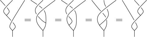
Figure 10.

Theorem 4.1.

There is a monomorphism $\iota_{R}:H^{2}_{\rm YBH}(V,V)\rightarrow H^{2}_{\rm YBH}(V_{R},V_{R})$.

Proof.

For $(\phi,\psi)\in C^{2}_{\rm YBH}(V,V)$ of $(V,\mu,R)$, define 2-cochains $(\phi_{R},\psi_{R})$ of $(V,\mu R,R)$ by $\psi_{R}:=\mu\phi+\psi R$ and $\phi_{R}:=\phi$, $(\psi_{R},\phi_{R})\in C^{2}_{\rm YBH}(V_{R},V_{R})$, as well as $f_{R}\in C^{1}_{\rm YBH}(V_{R},V_{R})$ by $f_{R}:=f$ for $f\in C^{1}_{\rm YBH}(V,V)$.

First we show that $(\phi_{R},\psi_{R})\in Z^{2}_{\rm YBH}(V_{R},V_{R})$. Each of associativity, Equation (1), and Equation (2) for $V_{R}$ follow from those of $V$. In the infinitesimal deformation $\tilde{V}$ of $V$, $(\mu+\hbar\psi,R+\hbar\phi)$ satisfies these relations, from the 2-cocycle relations of $(\phi,\psi)$. In order to show that $(\phi_{R},\psi_{R})$ satisfies the 2-cocycle conditions, it is sufficient to show that the infinitesimal deformation $\tilde{V}_{R}$ of $V_{R}$, $(\mu_{R}+\hbar\psi_{R},R+\hbar\phi_{R})$ satisfy the associativity, Equation (1) and Equation (2). We note that

$$\mu_{R}+\hbar\psi_{R}=\mu R+\hbar(\mu\phi+\psi R)\equiv(\mu+\hbar\psi)(R+\hbar\phi)\quad{\rm modulo}\quad(\hbar^{2}),$$

and $R+\hbar\phi_{R}=R+\hbar\phi$. Therefore the fact that the infinitesimal deformation $(\mu_{R}+\hbar\psi_{R},R+\psi_{R})$ giving a braided algebra modulo $(\hbar^{2})$ follows from the assumption that $(\mu+\hbar\psi,R+\hbar\phi)$ giving the infinitesimal deformation that is a braided algebra. Hence the claim follows.

Alternatively, it can be directly verified that 2-cocycle conditions for $(\phi,\psi)$ implies those for $(\phi_{R},\psi_{R})$ diagrammatically. For example, such computations for the Hochschild (associative) 2-cocycle condition are depicted in Figure 11. In the figure, the equalities $(A)$, $(B)$, $(C)$, $(D)$ are, respectively, the YI, Hochschild, Yang-Baxter, and IY 2-cocycle conditions.

To show that $\iota_{R}$ descends to cohomology, for $(\phi,\psi)=(\delta^{1}_{\rm YB}(f),\delta^{1}_{\rm H}(f))$, we compute

$$\psi_{R} = \iota_{R}(\delta^{1}_{\rm YB}(f),\delta^{1}_{\rm H}(f))$$

$$= [\mu R(f\otimes{\mathbb{1}})+\mu R({\mathbb{1}}\otimes f)-\mu(f\otimes{\mathbb{1}})R-\mu({\mathbb{1}}\otimes f)R]$$

$$+[\mu(f\otimes{\mathbb{1}})R+\mu({\mathbb{1}}\otimes f)R-f\mu R]$$

$$= \mu R(f\otimes{\mathbb{1}})+\mu R({\mathbb{1}}\otimes f)-f\mu R$$

$$= \delta^{1}_{\rm YBH}(f)$$

as desired. It is also clear that $\iota_{R}$ is a $\mathbb{k}$-module homomorphism. To show injectivity, assume that $(\phi_{R},\psi_{R})$ is a coboundary, that is, $\psi_{R}=\delta^{1}_{\rm H}(f)$ and $\phi_{R}=\delta^{1}_{\rm YB}(f)$. Since $\phi_{R}=\phi$, we have $\phi=\delta^{1}_{\rm YB}(f)$. From $\psi_{R}=\delta^{1}_{\rm H}(f)$ we obtain $\phi\mu+\psi R=\mu R(f\otimes{\mathbb{1}})+\mu R({\mathbb{1}}\otimes f)-f\mu R$. Substituting $\phi=\delta^{1}_{\rm YB}(f)$ in the left hand side, we obtain

$$[\mu R(f\otimes{\mathbb{1}})+\mu R({\mathbb{1}}\otimes f)-\mu(f\otimes{\mathbb{1}})R-\mu({\mathbb{1}}\otimes f)R]+\psi R=\mu R(f\otimes{\mathbb{1}})+\mu R({\mathbb{1}}\otimes f)-f\mu R,$$

which gives $\psi R=\mu(f\otimes{\mathbb{1}})R+\mu({\mathbb{1}}\otimes f)R-f\mu R$, and canceling the invertible $R$, we obtain $\psi=\delta^{1}_{\rm H}(f)$, thus $(\phi,\psi)$ is a coboundary. ∎

Inductively, we have the following.

Corollary 4.2.

If $H^{2}_{\rm YBH}(V,V)\neq 0$, then for all $n>0$, we have $H^{2}_{\rm YBH}(V_{R^{n}},V_{R^{n}})\neq 0$

Remark 4.3.

Corollary 4.2 shows that whenever we find a braided algebra $V$ with nontrivial YBH cohomology (as we do in Section 5), there are infinitely many braided algebras $V_{R^{n}}$ whose second YBH cohomology group is nontrivial as well.

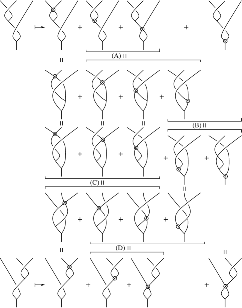
Figure 11.

5. Hopf algebra cohomology and braided algebra cohomology

In this section we construct a homomorphism between the second cohomology group of Hopf algebras and the second YBH cohomology of their corresponding braided algebras. Recall ([ChariPressley], Chapter 6) that the Hopf algebra second cohomology group with coefficients in $H$ characterizes Hopf algebra deformations. Roughly speaking, a $2$-cocycle for a Hopf algebra consists of a pair of cochains $(\xi,\zeta)$ such that $\xi$ deforms the algebra structure, $\zeta$ deforms the coalgebra structure, and such deformations are compatible.

We adopt the symbols $(\phi,\psi)$ for YBH 2-cocycles, and use $(\xi,\zeta)$ for Hopf algebra 2-cocycles, where $\xi\in{\rm Hom}(V^{\otimes 2},V)$ is a deformation 2-cocycle of a Hopf algebra multiplication $\mu$, and $\zeta\in{\rm Hom}(V,V^{\otimes 2})$ is a deformation 2-cocycle of a comultiplication $\Delta$. Both multiplications for braided algebras and Hopf algebras share the same symbol $\mu$, as it causes little confusion.

More specifically, Hopf algebra 2-cochain groups with coefficient group $H$ are defined as

$$C^{2}_{\rm Hf}(H,H)=C^{2,1}_{\rm Hf}(H,H)\oplus C^{2,2}_{\rm Hf}(H,H),$$

where $C^{2,1}_{\rm Hf}(H,H)={\rm Hom}(H,H^{\otimes 2})$ and $C^{2,2}_{\rm Hf}(H,H)={\rm Hom}(H^{\otimes 2},H)$. If $\mu$ and $\Delta$ denote the multiplication and comultiplication of a Hopf algebra $H$, the 2-cocycles $\xi\in Z^{2,1}_{\rm Hf}(H,H)$ and $\zeta\in Z^{2,2}_{\rm Hf}(H,H)$ deform $\mu$ and $\Delta$, respectively, so that $\tilde{\mu}=\mu+\hbar\xi$ and $\tilde{\Delta}=\Delta+\hbar\zeta$ defines a Hopf algebra structure on $H\otimes{\mathbb{k}}[[\hbar]]/(\hbar^{2})$. This condition requires that $(\xi,\zeta)$ satisfies the compatibility condition needed to guarantee that $\tilde{\Delta}\tilde{\mu}=(\tilde{\mu}\otimes\tilde{\mu})(\mathbb{1}\otimes\tau\otimes\mathbb{1})(\tilde{\Delta}\otimes\tilde{\Delta})$, where $\tau$ indicates transposition of tensor factors as before.

Let $H$ be a Hopf algebra and let $(\xi,\zeta)$ be a $2$-cocycle with coefficients in $H$. The $2$-cocycle condition for $\xi$ with coefficients in $H$ takes the form (on simple tensors)

$$\xi(x\otimes y)z+\xi(xy\otimes z)=x\xi(y\otimes z)+\xi(x\otimes yz).$$

The morphism $\zeta:H\rightarrow H\otimes H$ is a coalgebra cocycle (see [Doi]). That is, for every $x\in H$, $\zeta$ satisfies the equation

$$x^{(1)}\otimes\zeta(x^{(2)})+(\mathbb{1}\otimes\Delta)\zeta(x)=\zeta(x^{(1)})\otimes x^{(2)}+(\Delta\otimes\mathbb{1})\zeta(x).$$

Additionally, from imposing that the infinitesimal deformations $\xi$ and $\zeta$ are compatible – i.e. they define a bialgebra structure, one gets a compatibility condition involving both maps, namely

$$\Delta(\xi(x\otimes y))+\zeta(xy)=(\mu\otimes\xi+\xi\otimes\mu)\Delta^{13}(x)\Delta^{24}(y)+\zeta(x)\Delta(y)+\Delta(x)\zeta(y),$$

where we have used the definition $\Delta^{ij}(x)$ to indicate the $4$ components tensor with $\Delta(x)$ at entries $i$ and $j$, and $1$ elsewhere.

Remark 5.1.

Suppose that $(\xi,\zeta)$ is a Hopf algebra $2$-cocycle. Then, if $\tilde{\mu}$ and $\tilde{\Delta}$ are the corresponding deformed structures, from the property of the antipode of a Hopf algebra, which holds true for the deformed structure as well, we have that $\tilde{\mu}(\mathbb{1}\otimes S)\tilde{\Delta}(x)=\tilde{\mu}(S\otimes\mathbb{1})\tilde{\Delta}=\xi(1)$, which in degree $1$ in $\hbar$ gives the equality

$$\xi(x^{(1)}\otimes S(x^{(2)}))+\mu(\mathbb{1}\otimes S)\zeta(x)=\xi(S(x^{(1)})\otimes x^{(2)})+\mu(S\otimes\mathbb{1})\zeta(x)=0.$$

Observe that in the case $\zeta=0$ this gives us that $\xi(x^{(1)}\otimes S(x^{(2)}))=\xi(S(x^{(1)})\otimes x^{(2)})=0$.

For ease of notation, we will denote $\zeta(x)$ in Sweedler notation as for $\Delta$, the only difference being that we will use lower scripts for $\zeta$, while upper scripts for $\Delta$. Therefore, we will have $\zeta(x)=x_{(1)}\otimes x_{(2)}$. Since $(\Delta\otimes\mathbb{1})\zeta$ and $(\zeta\otimes\mathbb{1})\Delta$ are in general not the same, we introduce further a notation to distinguish the consecutive application of $\Delta$ and $\zeta$. We set

$$(\mathbb{1}\otimes\Delta)\zeta(x)=(\mathbb{1}\otimes\Delta)(x_{(1)}\otimes x_{(2)})=(x_{(1)})^{(1)}\otimes(x_{(1)})^{(2)}\otimes x_{(2)}=:\prescript{}{(1)}{x}\otimes\prescript{}{(2)}{x}\otimes\prescript{}{(3)}{x},$$

and similarly we set $(\mathbb{1}\otimes\zeta)\Delta(x)=:\prescript{(1)}{}{x}\otimes\prescript{(2)}{}{x}\otimes\prescript{(3)}{}{x}$. This notation allows us to forget the brackets that determine whether the internal index is lower or upper – i.e. whether we have applied $\Delta$ or $\zeta$ first.

Let $H$ denote a Hopf algebra and let $R_{H}$ be the YB operator defined through the adjoint map as in Section 2.3. Let $(\xi,\zeta)$ denote a Hopf algebra $2$-cocycle as described above. We define the cochain $\Psi_{\zeta}(\xi):H\otimes H\rightarrow H\otimes H$ as

$$\Psi_{\zeta}(\xi)(x\otimes y) = y^{(1)}\otimes S(y^{(2)})\xi(x\otimes y^{(3)})+y^{(1)}\otimes\xi(S(y^{(2)})\otimes xy^{(3)})$$

$$+\prescript{}{(1)}{y}\otimes S(\prescript{}{(2)}{y})x\prescript{}{(3)}{y}+\prescript{(1)}{}{y}\otimes S(\prescript{(2)}{}{y})x\prescript{(3)}{}{y}.$$

Definition 5.2.

Let $H$ be a Hopf algebra with an antipode $S$. A 1-cochain $f\in C^{1}_{\rm Hf}(H,H)$ is called $S$-commuting if it satisfies $fS=Sf:H\rightarrow H$. The set of all $S$-commutative 1-cochains form a subgroup, called $S$-commutative 1-cochain group and is denoted by $C^{1}_{\rm HfS}(H,H)$. The quotient $Z^{2,i}_{\rm Hf}(H,H)/\delta^{1}_{\rm H}(C^{1}_{\rm HfS}(H,H))$ is denoted by $H^{2}_{\rm HfS}(H,H)$, and it is called the $S$-commuting Hopf algebra 2-cohomology group. Similar names and notations apply to boundary and cocycle groups.

Lemma 5.3.

If $\xi\in Z^{2,1}_{\rm Hf}(H,H)$ and $\zeta\in Z^{2,2}_{\rm H}(H,H)$ are cobounded by an $S$-commuting $1$-cochain, i.e. $\xi=\delta^{1,1}_{\rm Hf}(f)$ and $\zeta=\delta^{1,2}_{\rm Hf}(f)$ for some $f\in C^{1}_{\rm HfS}(H,H)$, where $\delta^{1,1}_{\rm Hf}\in{\rm Hom}(H^{\otimes 2},H)$ and $\delta^{1,2}_{\rm Hf}\in{\rm Hom}(H,H^{\otimes 2})$, then $(\Psi_{\zeta}(\xi),\xi)$ is cobounded by $f$, $\Psi_{\zeta}(\xi)=\delta^{1}_{\rm YB}(f)$.

Proof.

One computes

$$\Psi_{\delta^{1,1}_{\rm Hf}(f)}(\delta^{1,2}_{\rm Hf}(f))(x\otimes y)$$

$$= [y^{(1)}\otimes S(y^{(2)})f(x)y^{(3)}+y^{(1)}\otimes S(y^{(2)})xf(y^{(3)})-y^{(1)}S(y^{(2)})xf(y^{(3)})]$$

$$+[y^{(1)}\otimes f(S(y^{(2)}))xy^{(3)}+y^{(1)}S(y^{(2)})xf(y^{(3)})-y^{(1)}\otimes f(S(y^{(2)})y^{(3)})]$$

$$+[y^{(1)}\otimes S(f(y^{(2)})^{(1)})xf(y^{(2)})^{(2)}-y^{(1)}\otimes S(f(y^{(2)}))xy^{(3)}-y^{(1)}\otimes S(y^{(2)})xf(y^{(3)})]$$

$$+[f(y)^{(1)}\otimes S(f(y)^{(2)})xf(y^{(2)})^{(2)}-y^{(1)}\otimes S(f(y^{(2)})^{(1)})xf(y^{(3)})-f(y^{(1)})\otimes S(y^{(2)})xy^{(3)}]$$

$$= \delta^{1}_{\rm YB}(f)(x\otimes y).$$

The terms $y^{(1)}\otimes f(S(y^{(2)}))xy^{(3)}$ and $y^{(1)}\otimes S(f(y^{(2)})^{(1)})xf(y^{(3)})$ cancel due to the $S$-commuting condition on $f$. The remaining terms can be seen to constitute $\delta^{1}_{\rm YB}(\Psi_{\zeta}(\xi))$, completing the proof. ∎

We note that this does not imply that $\Psi$ provides a chain map, since $f$ is restricted to $S$-commuting 1-cochains.

Theorem 5.4.

Let $H$, $(\xi,\zeta)$ and $\Psi_{\zeta}$ be as above. Then, for each $\zeta$, $\Psi_{\zeta}$ induces a well defined morphism of cohomology groups $H^{2}_{\rm HfS}(H,H)\rightarrow H^{2}_{\rm YBH}(H,H)$ between $S$-commuting Hopf cohomology and YBH cohomology.

Proof.

Since $\xi\in H^{2}_{\rm Hf}(H,H)$ is mapped to $\psi\in H^{2}_{\rm YBH}(H,H)$, and

$$\delta^{2,1}_{\rm Hf}(\xi)=\delta^{2}_{\rm H}(\psi),$$

if $\xi$ is a 2-cocycle, the corresponding $\psi$ is also a 2-cocycle.

We note that a $2$-cochain $\pi:H\otimes H\rightarrow H\otimes H$ is a YB $2$-cocycle for $R_{H}$ if and only if it is an infinitesimal deformation, i.e. if and only if $\tilde{R}=R_{H}+\hbar\pi$ is a YB operator for $H\otimes\mathbb{k}[[\hbar]]/(\hbar^{2})$. Let us consider the deformed structures $\tilde{\mu}=\mu+\hbar\xi$ and $\tilde{\Delta}=\Delta+\hbar\zeta$. They define a Hopf algebra structure (the infinitesimal deformation of $H$) since $(\xi,\zeta)$ is a Hopf $2$-cocycle by definition. Let $R_{\tilde{H}}$ be the YB operator defined through the adjoint map as in Section 2.3. Since $R_{\tilde{H}}$ can be written as $R_{\tilde{H}}=R_{H}+\hbar\Psi_{\zeta}(\xi)$ we have that $\Psi_{\zeta}(\xi)$ satisfies the YB $2$-cocycle condition, which shows that $(\Psi(\xi),\xi)$ is a braided algebra $2$-cocycle.

We apply the same argument to show that $(\Psi_{\zeta}(\xi),\xi)$ satisfy the YI and IY $2$-cocycle conditions. By Lemma 3.6, the deformations $\tilde{\mu}=\mu+\hbar\psi=\mu+\hbar(\xi)$ and $\tilde{R}=R+\hbar\Psi_{\zeta}(\xi)$ define a braided algebra if and only if $(\Psi_{\zeta}(\xi),\xi)$ is a YI and IY 2-cocycle. By Lemma 2.6, if $\tilde{\mu}$ and $\tilde{\Delta}$ define a (infinitesimal) Hopf algebra, then $\mu$ and the adjoint YB operator $\tilde{R}$ define a braided algebra. Hence $(\Psi_{\zeta}(\xi),\xi)$ is a YI and IY 2-cocycle. ∎

Remark 5.5.

We observe that although the map in Theorem 5.4 relates $S$-commuting Hopf cohomology group and YBH cohomology, a substantially identical proof shows that the same correspondence maps nontrivial Hopf algebra $2$-cocycles to nontrivial YBH $2$-cocycles. However, this mapping might not descend to a well defined map between cohomology groups. This observation is useful in the examples below.

Example 5.6.

By Theorem 3.8, if a cocycle deformation of a braided algebra by a pair of 2-cocycles $(\phi,\psi)$ defines a nontrivial deformation, then $(\phi,\psi)$ is a non-coboundary. While it is known that over fields of characteristic zero there are no nontrivial deformations for the group algebra [ChariPressley], for group algebras over more general rings there exist nontrivial deformations [SiegelWith]. Therefore, the corresponding braided algebras are deformed nontrivially. Hence in such cases the second cohomology group of YBH cohomology is nontrivial.

Example 5.7.

Let us now consider a more general setting than that of Example 5.6 above. For an algebraic group $G$, let $\mathcal{F}(G)$ denote the algebra of regular functions. Then it is known (see [ChariPressley]) that there are nontrivial deformations of $\mathcal{F}(G)$ as a Hopf algebra, though the coalgebra structure has trivial deformation. Applying Remark 5.5 we obtain nontrivial deformations (and therefore nontrivial elements in the braided algebra second cohomology group according to Theorem 3.8) of the associated braided algebra.

6. Third cohomology and quadratic deformations

In this section we consider the problem of extending an infinitesimal deformation to higher degrees in $\hbar$. In the case of associative algebras [Gerst] and Lie algebras [Nij-Rich], it is well known that the obstruction to extending an infinitesimal deformation to higher degrees lies in the third cohomology group of the algebra, therefore giving a simple criterion for the existence of such extensions. In fact, if the third cohomology group is trivial, it follows that any infinitesimal deformation can be extended. In this situation it is also said that the deformation is integrable. This holds true also when dealing with YB cohomology [Eisermann].

First we define the third cohomology groups for braided algebras, and then give their interpretation as obstructions to deformations.

6.1. The third differentials

Let $V$ be a braided algebra. We define

$$C^{4}_{\rm YI}(V,V)=C^{4,4}_{\rm YBH}(V,V)\oplus C^{4,3}_{\rm YI}(V,V)\oplus C^{4,2}_{\rm YI}(V,V)\oplus C^{4,2}_{\rm IY}(V,V)\oplus C^{4,1}_{\rm YBH}(V,V).$$

We define $\delta^{3}_{\rm YI}(V,V):C^{3}_{\rm YI}(V,V)\rightarrow C^{4}_{\rm YI}(V,V)$ by $\delta^{3}_{\rm YI}=\delta^{3}_{\rm YB}\oplus\delta^{3,1}_{\rm YI}\oplus\delta^{3,2}_{\rm YI}\oplus\delta^{3,3}_{\rm YI}\oplus\delta^{3}_{\rm H}$, where each direct summand of the differential is defined as follows. For $\alpha\in C^{3,2}_{\rm YI}(V,V)$ and $\beta\in C^{3,3}_{\rm YBH}(V,V)$, define $\delta^{3,1}_{\rm YI}:C^{3,3}_{\rm YBH}(V,V)\oplus C^{3,2}_{\rm YI}(V,V)\rightarrow C^{4,3}_{\rm YI}(V,V)$ by

$$\delta^{3,1}_{\rm YI}(\beta\oplus\alpha) = ({\mathbb{1}}\otimes R)(\alpha\otimes{\mathbb{1}})({\mathbb{1}}^{\otimes 2}\otimes R)+({\mathbb{1}}\otimes\alpha)(R\otimes{\mathbb{1}}^{\otimes 2})({\mathbb{1}}\otimes R\otimes{\mathbb{1}})({\mathbb{1}}^{\otimes 2}\otimes R)$$

$$+({\mathbb{1}}^{\otimes 2}\otimes\mu)({\mathbb{1}}\otimes R\otimes{\mathbb{1}})(R\otimes{\mathbb{1}}^{\otimes 2})({\mathbb{1}}\otimes\beta)+({\mathbb{1}}^{\otimes 2}\otimes\mu)(\beta\otimes{\mathbb{1}})({\mathbb{1}}^{\otimes 2}\otimes R)({\mathbb{1}}\otimes R\otimes{\mathbb{1}})$$

$$-\beta(\mu\otimes{\mathbb{1}}^{\otimes 2})-({\mathbb{1}}\otimes R)(R\otimes{\mathbb{1}})(\alpha\otimes{\mathbb{1}})-(R\otimes\mathbb{1})(\mathbb{1}\otimes\alpha)(R\otimes\mathbb{1}^{\otimes 2})(\mathbb{1}\otimes R\otimes\mathbb{1}).$$

Define $C^{3,2}_{\rm YI}(V,V)\oplus C^{3,2}_{\rm IY}(V,V)\rightarrow C^{4,2}_{\rm IY}(V,V)$ for $\alpha\in C^{3,2}_{\rm YI}(V,V)$ and $\alpha^{\prime}\in C^{3,2}_{\rm IY}(V,V)$ by

$$\delta^{3,2}_{\rm YI}(\alpha\oplus\alpha^{\prime}) = (\mu\otimes{\mathbb{1}}^{\otimes 2})\alpha^{\prime}+(\alpha\otimes{\mathbb{1}})({\mathbb{1}}\otimes R)((\mu\otimes{\mathbb{1}})+({\mathbb{1}}\otimes R\otimes{\mathbb{1}})(R\otimes{\mathbb{1}}^{\otimes 2}))({\mathbb{1}}\otimes\alpha)(\mu\otimes{\mathbb{1}})$$

$$-({\mathbb{1}}^{\otimes 2}\otimes\mu)\alpha-({\mathbb{1}}\otimes\alpha^{\prime})(R\otimes{\mathbb{1}})({\mathbb{1}}\otimes\mu)-({\mathbb{1}}\otimes R\otimes{\mathbb{1}})({\mathbb{1}}^{\otimes 2}\otimes R)(\alpha^{\prime}\otimes{\mathbb{1}})({\mathbb{1}}\otimes\mu).$$

Define further $\delta^{3,3}_{\rm YI}:C^{3,2}_{\rm YBH}(V,V)\oplus C^{3,1}_{\rm YBH}(V,V)\rightarrow C^{4,2}_{\rm YBH}(V,V)$ for $\alpha\in C^{3,2}_{\rm YBH}(V,V)$ and $\gamma\in C^{3,1}_{\rm YBH}(V,V)$ by

$$\delta^{3,3}_{\rm YI}(\alpha\oplus\gamma) = (\gamma\otimes{\mathbb{1}})R+({\mathbb{1}}\otimes\mu)\alpha+({\mathbb{1}}\otimes\alpha)(R\otimes{\mathbb{1}})\mu$$

$$-(\mu\otimes{\mathbb{1}})\alpha-({\mathbb{1}}^{\otimes 2}\otimes R)(\alpha\otimes{\mathbb{1}}^{\otimes 2})\mu-({\mathbb{1}}^{\otimes 2}\otimes R)({\mathbb{1}}\otimes R\otimes{\mathbb{1}})(R\otimes{\mathbb{1}}^{\otimes 2})\gamma.$$

The differentials $\delta^{3,i}_{\rm YI}$, $i=1,2,3$, have diagrammatic representations depicted in Figures 12, 13, and 14, respectively. In Figure 12, from the top initial diagram labeled (I) to the bottom terminal figure labeled (T) there are two sequences of equalities that use Equation (1) . The two sequences are labeled for left hand side and right hand side by $(L1)$, $(L2)$, $(L3)$ and $(R1)$, $(R2)$, respectively. Between (I) and (L1), a trivalent vertex goes through an over-arc at a crossing, introducing two crossings in (L1). At the moment when the trivalent vertex and a crossing merge, a 5-valent vertex appears as depicted in (LD1) marked by a small circle. This circled 5-valent vertex with top 3 edges and bottom 2 segments represents $\alpha\in C^{3,2}_{\rm YBH}(V,V)={\rm Hom}_{\mathbb{k}}(V^{\otimes 3},V^{\otimes 2})$. When the diagram of (LD1) is read from top to bottom, there is a crossing at the top with two parallel lines to its left. This represents the first factor $({\mathbb{1}}\otimes R)$ in the first term of $\delta^{3,1}_{\rm YI}(\beta\oplus\alpha)$. The second factor $(\alpha\otimes{\mathbb{1}})$ represents the 5-valent vertex with one string to the right, and the last factor $({\mathbb{1}}^{\otimes 2}\otimes R)$ represents the crossing at the bottom of (LD1). The four positive terms in $\delta^{3,1}_{\rm YI}(\beta\oplus\alpha)$ are represented by (LD$n$) for $n=1,2,3,4$ in this order, and the negative terms are represented by the right hand side diagrams (RD$n$) for $n=1,2$.

Figure 12.

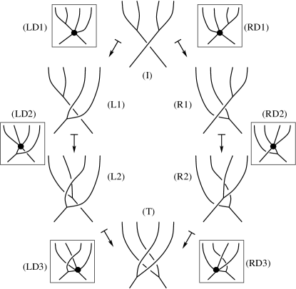
Figure 13.

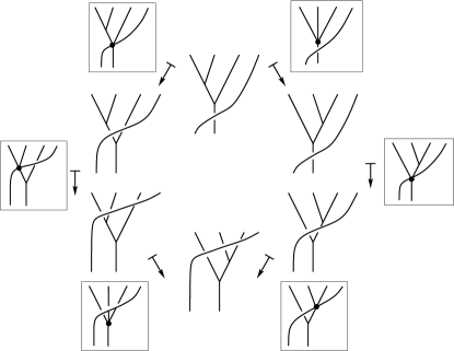
Figure 14.

Proposition 6.1.

The sequence

$$C_{\rm YBH}^{2}(V,V)\stackrel{{\scriptstyle\delta^{2}_{\rm YBH}}}{{\longrightarrow}}C_{\rm YBH}^{3}(V,V)\stackrel{{\scriptstyle\delta^{3}_{\rm YI}}}{{\longrightarrow}}C_{\rm YI}^{4}(V,V)$$

forms a cochain complex.

Proof.

We show that $\delta^{3,2}_{\rm YI}(\alpha\oplus\alpha^{\prime})=0$, $\alpha=\delta^{2}_{\rm YI}(\psi\oplus\phi)$ and $\alpha^{\prime}=\delta^{2}_{\rm IY}(\psi\oplus\phi)$. We use the diagrammatics in Figure 15. The 3-cochain $\alpha^{\prime}$ is represented by a circled 4-valent (3 in, 1 out) vertex in the diagram (1). The assumption $\alpha^{\prime}=\delta^{2}_{\rm IY}(\psi\oplus\phi)$ is represented by the right side of the figure with labels (1-1), (1-2), (2-1), (2-2) and (2-3), where the linear combination of the terms (1-1) $+$ (1-2) $-$ (2-1) $-$ (2-2) $-$ (2-3) represents the assumed 2-cocycle condition. Similarly (2) represents $\alpha$ and (2-4) $+$ (2-5) $-$ (3-1) $-$ (3-2) $-$ (3-3) represents $\alpha=\delta^{2}_{\rm YI}(\psi\oplus\phi)$. One finds the canceling pair (2-1) and (2-5). One finds each circled 4-valent vertex appearing in the same position twice, they cancel in pairs, indicating $\delta^{3,2}_{\rm IY}(\alpha\oplus\alpha^{\prime})=0$. The other cases are similar. ∎

Similar definitions where the IY condition is used instead of the YI condition give a differential $\delta^{3}_{\rm IY}$. As it will be proved below, they contain the obstructions to higher order deformations corresponding to Equation (1) and Equation (2), respectively.

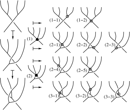
Figure 15.

6.2. Quadratic deformation for Hochschild cohomology

In this section we review the second degree deformations and the third cohomology group of associative algebras [Gerst]. These methods are applied in the following section to develop an analogous theory for Yang-Baxter Hochschild cohomology. We provide a diagrammatic proof of a known result in Appendix A, which will be used to prove the results of Section 6.3.

Let $(V,\mu)$ be an algebra over ${\mathbb{k}}$, and let $\psi=\psi_{1}$ denote a Hochschild $2$-cocycle, $\psi_{1}\in Z^{2}_{\rm H}(V,V)$. As before we set $(\tilde{V},\tilde{\mu})$, where $\tilde{V}=V\otimes{\mathbb{k}}[[\hbar]]/(\hbar^{2})$ and $\tilde{\mu}=\mu+\hbar\psi_{1}$. Next we consider $(\hat{V},\hat{\mu})$ where $\hat{V}=V\otimes{\mathbb{k}}[[\hbar]]/(\hbar^{3})$ and $\hat{\mu}=\mu+\hbar\psi_{1}+\hbar^{2}\psi_{2}$. One computes the degree two term of $\hbar$ to be

$$\hbar^{2}[\{\mu(\psi_{2}\otimes\mathbb{1})+\psi_{2}(\mu\otimes\mathbb{1})-\mu(\mathbb{1}\otimes\psi_{2})-\psi_{2}(\mathbb{1}\otimes\mu))\}+\{\psi_{1}(\psi_{1}\otimes\mathbb{1})-\psi_{1}(\mathbb{1}\otimes\psi_{1}))\}]$$

$$=\hbar^{2}[\delta^{2}(\psi_{2})+\{\psi_{1}(\psi_{1}\otimes\mathbb{1})-\psi_{1}(\mathbb{1}\otimes\psi_{1})\}].$$

Set $\Theta_{2}(\psi_{1})=\psi_{1}(\psi_{1}\otimes\mathbb{1})-\psi_{1}(\mathbb{1}\otimes\psi_{1})$. Then this computation shows the following.

Lemma 6.2.

The above defined $(\hat{V},\hat{\mu})$ is an algebra such that $\hat{\mu}\equiv_{(\hbar^{2})}\mu$ if and only if $\delta^{2}(\psi_{2})+\Theta_{2}(\psi_{1})=0$.

In this case we say that $(\hat{V},\hat{\mu})$ is a degree 2 deformation of $(V,\mu)$. Next, we recall the following.

Lemma 6.3 ([Gerst]).

$\delta^{3}_{\rm H}\Theta_{2}(\psi_{1})=0$.

By this lemma, $\Theta_{2}(\psi_{1})$ is a Hochschild 3-cocycle, representing an element $[\Theta_{2}(\psi_{1})]\in H^{3}_{\rm H}(V,V)$. If $\delta^{2}(\psi_{2})+\Theta_{2}(\psi_{1})=0$ as in Lemma 6.2, then $\Theta_{2}(\psi_{1})$ is a coboundary, $[\Theta_{2}(\psi_{1})]=0$, and the degree 1 deformation $(\tilde{V},\tilde{\mu})$ of $(V,\mu)$ further deforms to $(\hat{V},\hat{\mu})$. In particular, if $H^{3}(V,V)=0$, then $(V,\mu)$ deforms to $(\hat{V},\hat{\mu})$. Thus $H^{3}(V,V)$ can be regarded as obstruction to quadratic deformation.

We provide a diagrammatic proof of Lemma 6.3 in Appendix A. We use similar techniques for the third Yang-Baxter Hochschild cohomology group in the following section.

Lastly, we hereby recall the obstruction to higher degree deformations for associative algebras, as it motivates some of the results found below (see Theorem 6.5). In fact, suppose $(A,\mu)$ is an algebra and $\hat{\mu}=\sum_{i=0}^{k}\hbar^{i}\mu_{i}$ is a deformation of degree $k$ (here $\mu_{0}=\mu$). Consider the degree $k+1$ deformation $\tilde{\mu}=\hat{\mu}+\hbar^{k+1}\mu_{k+1}$. Then, the associativity condition for $\tilde{\mu}$ is automatically satisfied in degree at most $k$, while in degree $k+1$ takes the form

$$\sum_{t=1}^{k}\mu_{t}(\mu_{k+1-t}\otimes\mathbb{1})+\mu_{0}(\mu_{k+1}\otimes\mathbb{1})+\mu_{k+1}(\mu_{0}\otimes\mathbb{1})$$

$$= \sum_{t=1}^{k}\mu_{t}(\mathbb{1}\otimes\mu_{k+1-t})+\mu_{0}(\mathbb{1}\otimes\mu_{k+1})+\mu_{k+1}(\mathbb{1}\otimes\mu_{0}),$$

which can be rewritten as

$$\delta_{H}^{2}(\mu_{k+1})+\Theta_{k+1}=0,$$

where $\Theta_{k+1}$ contains terms not involving $\mu_{k+1}$. Similarly as above, it holds that $\delta^{3}_{H}(\Theta_{k+1})=0$, and the obstruction to extend a degree $k$ deformation to a degree $k+1$ deformation lies in the third cohomology group [Gerst].

In this case we do not provide a diagrammatic proof of these classic results, as the analogue approach for braided algebras becomes increasingly complicated to handle. However, we expect that the results below that show that the obstruction for degree $2$ deformations lie in the third cohomology group of braided algebras, would extend to the case of higher degree deformations as in the case of associative algebras.

6.3. Higher order deformations for Yang-Baxter Hochschild homology

We investigate the obstructions to higher deformations for braided algebras, and obtain integrability criteria at least in some special cases of interest. This requires additional obstructions for the compatibility among higher degree deformation terms lying in the third YBH cohomology groups. First, we pose the following inductive definition, where Defintion 3.4 serves as the base case $n=1$.

Definition 6.4.

Let $(V,\mu,R)$ be a braided algebra, and let $(\tilde{V},\tilde{\mu},\tilde{R})$ be a deformation of degree $n$. Then, we say that $(\hat{V},\hat{\mu},\hat{R},)$ is a deformation of $(V,\mu,R)$ of order $n+1$ if it is a braided algebra over the ring $\mathbb{k}[[\hbar]]/(\hbar^{n+2})$ and, in addition, $\hat{R}\cong_{(\hbar^{n+1})}\tilde{R}$ and $\hat{\mu}\cong_{(\hbar^{n+1})}\tilde{\mu}$.

We will use the notation $R_{n}=\sum_{i=0}^{n}\hbar^{i}\phi_{i}$ and $\mu_{n}=\sum_{i=0}^{n}\hbar^{i}\psi_{i}$, where $\phi_{0}:=R$ and $\psi_{0}:=\mu$. For all $r\geq 2$ we also set the triples of integers

$$\Gamma_{r}:=\{(i,j,k)\ |\ i+j+k=r,\ i,j,k\geq 0,\ i,j,k\neq r\}.$$

Then, we define

$$\Xi^{\rm YI}_{r}:=\sum_{(i,j,k)\in\Gamma_{r}}(\psi_{i}\otimes\mathbb{1})(\mathbb{1}\otimes\phi_{j})(\phi_{k}\otimes 1), \Omega^{\rm YI}_{r}:=\sum_{(p,q,0)\in\Gamma_{r}}\phi_{p}(\mathbb{1}\otimes\psi_{q}),$$

$$\Xi^{\rm IY}_{r}:=\sum_{(i,j,k)\in\Gamma_{r}}(\mathbb{1}\otimes\psi_{i})(\phi_{j}\otimes\mathbb{1})(\mathbb{1}\otimes\phi_{k}), \Omega^{\rm IY}_{r}:=\sum_{(p,q,0)\in\Gamma_{r}}\phi_{p}(\psi_{q}\otimes\mathbb{1}).$$

Lastly, we define

$$\Theta_{r}=\sum_{(i,j,k)\in\Gamma_{r}}(\phi_{i}\otimes\mathbb{1})(\mathbb{1}\otimes\phi_{j})(\phi_{k}\otimes\mathbb{1})-(\mathbb{1}\otimes\phi_{i})(\phi_{j}\otimes\mathbb{1})(\mathbb{1}\otimes\phi_{k})$$

and $\Lambda_{r}=\sum_{(p,q,0)\in\Gamma_{r}}\mu_{p}(\mu_{q}\otimes\mathbb{1})-\mu_{p}(\mathbb{1}\otimes\mu_{q})$.

Theorem 6.5.

Let $(V,\mu,R)$ be a braided algebra, and let $(\tilde{V},\mu_{n},R_{n})$ be a deformation of degree $n$. Then $(V,\mu_{n+1},R_{n+1})$ is a deformation of $(V,\mu,R)$ of order $n+1$ if and only if

$\begin{cases}\delta^{2}_{\rm YB}\phi_{n+1}+\Theta_{n+1}=0\\ \delta^{2}_{\rm YI}(\phi_{n+1},\psi_{n+1})+\Xi^{\rm YI}_{n+1}-\Omega^{\rm YI}_{n+1}=0\\ \delta^{2}_{\rm IY}(\phi_{n+1},\psi_{n+1})+\Xi^{\rm IY}_{n+1}-\Omega^{\rm IY}_{n+1}=0\\ \delta^{2}_{\rm H}\psi_{n+1}+\Lambda_{n+1}=0.\end{cases}$

Proof.

The proof consists of some straightforward, albeit long, computations. We show some details regarding the second equation. We set $R_{n+1}=\sum_{i=0}^{n+1}\hbar^{i}\phi_{i}$ and $\mu_{n+1}=\sum_{i=0}^{n+1}\hbar^{i}\mu_{i}$, as above. Since by hypothesis $(R_{n},\mu_{n})$ defines a braided algebra deformation of $(V,\mu,R)$, Equation (1) on $R_{n+1}$ and $\mu_{n+1}$ gives an obstruction only on terms of degree $n+1$ in $\hbar$. Then, writing only the terms of degree $n+1$ in $\hbar$ we have

$$0 = (\psi_{n+1}\otimes\mathbb{1})(\mathbb{1}\otimes\phi_{0})(\phi_{0}\otimes\mathbb{1})+(\psi_{0}\otimes\mathbb{1})(\mathbb{1}\otimes\phi_{n+1})(\phi_{0}\otimes\mathbb{1})+(\psi_{0}\otimes\mathbb{1})(\mathbb{1}\otimes\phi_{0})(\phi_{n+1}\otimes\mathbb{1})$$

$$+\sum_{(i,j,k)\in\Gamma_{n+1}}(\psi_{i}\otimes\mathbb{1})(\mathbb{1}\otimes\phi_{j})(\phi_{k}\otimes\mathbb{1})-\sum_{(p,q,0)\in\Gamma_{n+1}}\phi_{p}(\mathbb{1}\otimes\psi_{q})$$

$$= \delta^{2}_{\rm IY}(\phi,\psi)+\Xi^{\rm IY}_{n+1}-\Omega^{\rm IY}_{n+1},$$

which is the second equation. Therefore, $(V,\mu_{n+1},R_{n+1})$ satisfies Equation 1 if and only if

$$\delta^{2}_{\rm YI}(\phi_{n+1},\psi_{n+1})+\Xi^{\rm YI}_{n+1}-\Omega^{\rm YI}_{n+1}=0$$

is satisfied. The other cases are treated analogously by direct inspection. ∎

Lemma 6.6.

The obstruction to extending an infinitesimal deformation of braided algebras to a quadratic deformation lies in the third YBH cohomology group. More concisely, we have

$$\delta_{\rm YBH}^{3}(\Theta_{2})=\delta_{\rm YBH}^{3}(\Xi^{\rm YI}_{2}-\Omega^{\rm YI}_{2})=\delta_{\rm YBH}^{3}(\Xi^{\rm IY}_{2}-\Omega^{\rm IY}_{2})=\delta_{\rm YBH}^{3}(\Lambda_{2})=0.$$

Proof.

The proof is given in Appendix B. ∎

The following result follows immediately from Lemma 6.6.

Corollary 6.7.

If $H_{\rm YBH}^{3}(V,V)=0$, then any infinitesimal deformation can be extended to a quadratic deformation.

Proof.

By Lemma 6.6, $\Theta_{2}$, $\Xi^{\rm YI}_{2}-\Omega^{\rm YI}_{2}$, $\Xi^{\rm IY}_{2}-\Omega^{\rm IY}_{2}$, and $\Lambda_{2}$ are 3-cocycles, representing elements of $H^{3}_{\rm YBH}(V,V)$. If the equalities in Theorem 6.5 hold, then these 3-cocycles are coboundaries. In particular, if $H_{\rm YBH}^{3}(V,V)=0$, then $(V,\mu,R)$ deforms to $(\hat{V},\hat{\mu},\hat{R})$. Thus, if $H^{3}_{\rm YBH}(V,V)=0$ there is no obstruction to extending an infinitesimal deformation to a quadratic deformation. ∎

Appendix A Proof of Lemma 6.3

This is a well known result in the literature, and the innovative component of this proof is a purely diagrammatic approach, which is employed extensively in the proofs in Appendix B.

In Figure 16, the pentagonal diagram is depicted that represents the Hochschild 3-cocycle condition. The leftmost tree represents the parenthesis structure $((xy)z)w$ for algebra monomials $x,y,z,w$, and the vertices of the pentagon list all possibilities of parentheses structures. Applying associativity corresponds to each directed edge, which represents a 3-cocycle $\alpha$ as depicted. The arguments involved in the associativity, $x,y,z$, are substituted in the 3-cocycle as depicted. The figure indicates that the Hochschild 3-cocycle condition corresponds to this figure.

\begin{overpic}[width=180.67499pt]{figures/hoch3}\put(-1.0,39.0){$x\ \,y\ \,z\ \,w$} \put(-5.0,69.0){$\alpha(x\otimes y\otimes z)w$} \put(31.0,80.0){$\alpha(x\otimes yz\otimes w)$} \put(66.0,69.0){$x\alpha(y\otimes z\otimes w)$} \put(7.0,-4.5){$\alpha(xy\otimes z\otimes w)$} \put(58.0,-4.5){$\alpha(x\otimes y\otimes zw)$} \end{overpic}

Figure 16.

Figure 17.

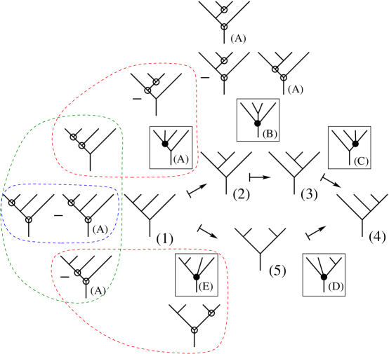
Figure 18.

Figure 19.

In Figure 17 (1), the substitution of the term $\psi_{1}(\psi_{1}\otimes{\mathbb{1}})-\psi_{1}({\mathbb{1}}\otimes\psi_{1})$ into a 3-cocycle, $\alpha(\psi_{1})=\psi_{1}(\psi_{1}\otimes{\mathbb{1}})-\psi_{1}({\mathbb{1}}\otimes\psi_{1})$, is depicted, where a white circle represents $\psi_{1}$. At each tree diagram of the pentagon, we place all possible pairs of circles to trivalent vertices, as depicted in (2), and make a formal linear combination with $\pm$ signs. In (2), the first two terms appear as the first term of (1), the second term appears in the $3$-cocycle labeled (E) in Figure 18, and the last two canceling pairs do not appear in 3-cocycle terms. All terms cancel as follows.

In Figure 18, the circled tree diagrams are depicted at the left most tree diagram. The red dotted circle at the 3-cocycle diagram represents the group of two diagrams in Figure 17 (1). One of them is a circled diagram of the tree (1) in Figure 18, and the other term corresponds to the tree (2). The blue dotted circle groups a canceling pair. The green dotted circle represents all circled tree diagrams of the tree (1), as depicted in Figure 17 (2). The bottom red circle represents the substitution of the 3-cocycle condition depicted in (E).

In Figure 19, all circled diagrams from all tree diagrams are depicted. The formal sum of all these terms corresponds to the differential of $\Theta_{2}(\psi_{1})$, and we show that this sum vanishes. This follows from the 2-cocycle condition of $\psi_{1}$. An incident of a 2-cocycle condition is depicted in Figure 17 (3), for the tree diagram Figure 18 (1). In Figure 17 (4), the 2-cocycle condition with an additional circle is depicted, which also vanishes. This vanishing equality (4) corresponds to Figure 18 (A), and its terms are depicted in Figure 18 with label (A). Thus the sum of the four circled tree diagrams labeled in Figure 18 vanishes by the 2-cocycle condition.

In Figure 19, all terms on the right-hand side are labeled by (A) through (E). The four terms together labeled by the same letter, then, vanish by the 2-cocycle condition, completing the proof.

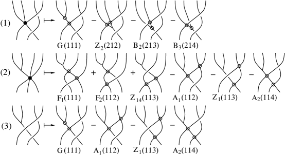
Figure 20.

Appendix B Proof of Lemma 6.6

The proof follows an argument similar to Lemma 6.2. The 3-cocycle $\alpha$ and $\beta$ are represented by black vertices of valency 2 and 3, respectively, in square-framed diagrams in Figure 12. The first term $(LD1)$ of the differential on the left hand side represents $({\mathbb{1}}\otimes R)(\alpha\otimes{\mathbb{1}})({\mathbb{1}}^{\otimes 2}\otimes R)$. The 3-cocycle condition $\delta^{3}_{\rm YI}(\beta\oplus\alpha)=0$ is represented by the expression $(LD1)+(LD2)+(LD3)+(LD4)-(RD1)-(RD2)-(RD3)$.

In Figure 20 (1), the first term $(LD1)$ in Figure 12 for a 3-cocycle condition of YI algebra is depicted at the left hand side. The labels are used later. We substitute $\Xi^{\rm YI}_{2}-\Omega^{\rm YI}_{2}$ for $\alpha$ in the term $(LD1)$, then we obtain maps represented by the right hand side of Figure 20 (1). Similarly, when we substitute $\Xi^{\rm YI}_{2}-\Omega^{\rm YI}_{2}$ for $\beta$ in $(RD1)$ in Figure 12, then we obtain the right hand side of Figure 20 (2). When these terms in (1) and (2) that have two circles on the diagrams in $(I)$, in Figure 12, then we obtain the right hand side of Figure 20 (3). This list in the right hand side of Figure 20 (3) appear in Figure 21 at the top left, above the dotted line. Below the dotted line are canceling pairs that are used to apply 3-cocycle conditions.

All terms, represented by square-framed diagrams in Figure 12, that appear in the 3-cocycle condition, are substituted with $\Xi^{\rm YI}_{2}-\Omega^{\rm YI}_{2}$, and grouped together according to each diagram of Figure 12, from the initial diagram (I) to the terminal diagram (T) through $(L1)$ through $(L3)$ and back to (I) through $(R2),(R1)$, in Figures 21 through 23 above the dotted lines. The terms in the right hand side $(R1)$ and $(R2)$ receive negative signs (left hand side - right hand side).

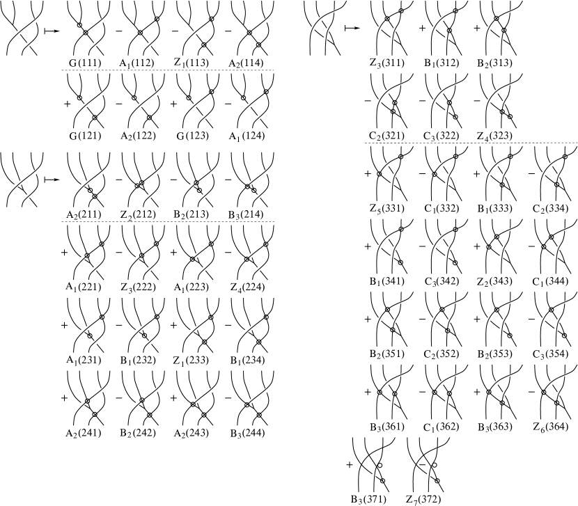
Figure 21.

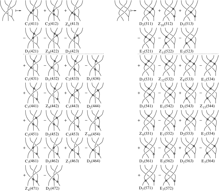
Figure 22.

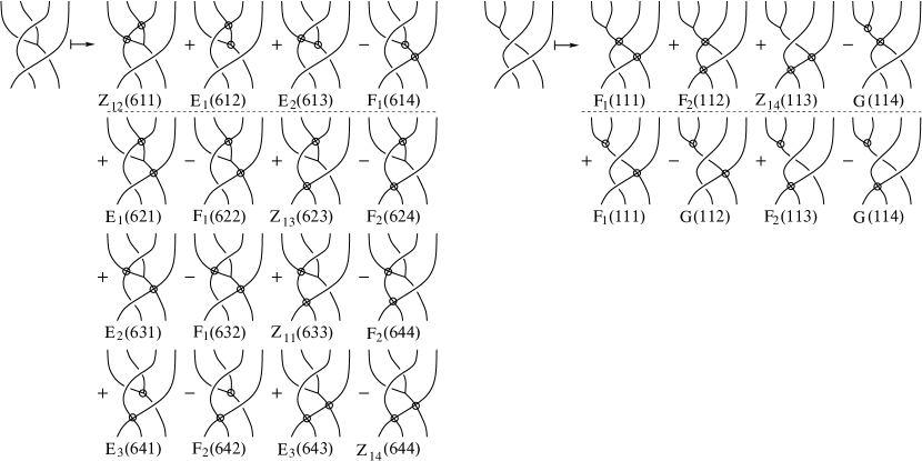
Figure 23.

In Figure 24, are listed the 3-cocycle conditions that are used to show that the sum of all terms vanish. In Figure 25, two examples (top two rows) of these 3-cocycle conditions are depicted in the right hand side. Each term is labeled as follows. The first letter $(A_{1})$ represents which 3-cocycle condition is used. The leftmost digit of the three digits represents the figure number counted from Figure 21 through Figure 23. The remaining two digits represent the row-column position. Therefore the labels in the terms in Figure 21 through Figure 23 shows that all these terms cancel by the 3-cocycle conditions, and cancelations with opposite signs such as the pair depicted in Figure 25 bottom row. These canceling terms are labeled by $Z$ with subscripts. Thus the vanishing of the total sum is checked by labels of diagrams, and the other cases are similarly checked.

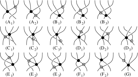
Figure 24.

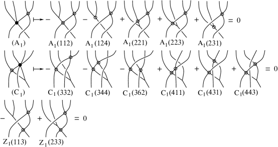
Figure 25.

References

- [1] 3-lie algebras, ternary nambu-lie algebras and the yang-baxter equationAbramovViktorZappalaEmanueleJ. Geom. Phys.183Paper No. 104687, 19pp2023Elsevier@article{AZ, title = {3-Lie algebras, ternary Nambu-Lie algebras and the Yang-Baxter equation}, author = {Abramov, Viktor}, author = {Zappala, Emanuele}, journal = {J. Geom. Phys.}, volume = {183}, pages = {Paper No. 104687, 19pp}, year = {2023}, publisher = {Elsevier}}
- [3] Hochschild homology in a braided tensor categoryBaezJohn C.Trans. Amer. Math. Soc.3442885–9061994@article{Baez, title = {Hochschild homology in a braided tensor category}, author = {Baez, John C.}, journal = {Trans. Amer. Math. Soc.}, volume = {344}, number = {2}, pages = {885–906}, year = {1994}}
- [5] BrownKenneth S.Cohomology of groupsGraduate Texts in Mathematics87Corrected reprint of the 1982 originalSpringer-Verlag, New York1994@book{Brown, author = {Brown, Kenneth S.}, title = {Cohomology of groups}, series = {Graduate Texts in Mathematics}, volume = {87}, note = {Corrected reprint of the 1982 original}, publisher = {Springer-Verlag, New York}, year = {1994}}
- [7] CarterJ. ScottCransAlissa S.ElhamdadiMohamedSaitoMasahicoCohomology of categorical self-distributivityJ. Homotopy Relat. Struct.Journal of Homotopy and Related Structures32008113–63@article{CCES-coalgebra, author = {Carter, J. Scott}, author = {Crans, Alissa S.}, author = {Elhamdadi, Mohamed}, author = {Saito, Masahico}, title = {Cohomology of categorical self-distributivity}, journal = {J. Homotopy Relat. Struct.}, fjournal = {Journal of Homotopy and Related Structures}, volume = {3}, year = {2008}, number = {1}, pages = {13–63}}
- [9] CarterJ. ScottCransAlissa S.ElhamdadiMohamedSaitoMasahicoCohomology of the adjoint of Hopf algebrasJ. Gen. Lie Theory Appl.Journal of Generalized Lie Theory and Applications22008119–34@article{CCES-adjoint, author = {Carter, J. Scott}, author = {Crans, Alissa S.}, author = {Elhamdadi, Mohamed}, author = {Saito, Masahico}, title = {Cohomology of the adjoint of {H}opf algebras}, journal = {J. Gen. Lie Theory Appl.}, fjournal = {Journal of Generalized Lie Theory and Applications}, volume = {2}, year = {2008}, number = {1}, pages = {19–34}}
- [11] CarterJ. ScottCransAlissa S.ElhamdadiMohamedSaitoMasahicoHomology theory for the set-theoretic Yang-Baxter equation and knot invariants from generalizations of quandlesFund. Math.Fundamenta Mathematicae184200431–54@article{CCES1, author = {Carter, J. Scott}, author = {Crans, Alissa S.}, author = {Elhamdadi, Mohamed}, author = {Saito, Masahico}, title = {Homology theory for the set-theoretic {Y}ang-{B}axter equation and knot invariants from generalizations of quandles}, journal = {Fund. Math.}, fjournal = {Fundamenta Mathematicae}, volume = {184}, year = {2004}, pages = {31–54}}
- [13] Quandle cohomology and state-sum invariants of knotted curves and surfacesCarterJ. ScottJelsovskyDanielKamadaSeiichiLangfordLaurelSaitoMasahicoTrans. Amer. Math. Soc.355103947–39892003@article{CJKLS, title = {Quandle cohomology and state-sum invariants of knotted curves and surfaces}, author = {Carter, J. Scott}, author = {Jelsovsky, Daniel}, author = {Kamada, Seiichi}, author = {Langford, Laurel}, author = {Saito, Masahico}, journal = {Trans. Amer. Math. Soc.}, volume = {355}, number = {10}, pages = {3947–3989}, year = {2003}}
- [15] CarterJ. ScottIshiiAtsushiSaitoMasahicoTanakaKokoroHomology for quandles with partial group operationsPacific J. Math.Pacific Journal of Mathematics2872017119–48@article{CIST, author = {Carter, J. Scott}, author = {Ishii, Atsushi}, author = {Saito, Masahico}, author = {Tanaka, Kokoro}, title = {Homology for quandles with partial group operations}, journal = {Pacific J. Math.}, fjournal = {Pacific Journal of Mathematics}, volume = {287}, year = {2017}, number = {1}, pages = {19–48}}
- [17] A guide to quantum groupsChariVyjayanthiPressleyAndrew1995Cambridge university press@book{ChariPressley, title = {A guide to quantum groups}, author = {Chari, Vyjayanthi}, author = {Pressley, Andrew}, year = {1995}, publisher = {Cambridge university press}}
- [19] Homological coalgebraDoiYukioJ. Math. Soc. Japan33131–501981@article{Doi, title = {Homological coalgebra}, author = {Doi, Yukio}, journal = {J. Math. Soc. Japan}, volume = {33}, number = {1}, pages = {31–50}, year = {1981}}
- [21] EisermannMichaelYang-Baxter deformations and rack cohomologyTrans. Amer. Math. Soc.3662014105113–5138@article{Eisermann, author = {Eisermann, Michael}, title = {Yang-{B}axter deformations and rack cohomology}, journal = {Trans. Amer. Math. Soc.}, volume = {366}, year = {2014}, number = {10}, pages = {5113–5138}}
- [23] Yang–baxter deformations of quandles and racksEisermannMichaelAlgebr. Geom. Topol.52537–5622005Mathematical Sciences Publishers@article{Eisermann1, title = {Yang–Baxter deformations of quandles and racks}, author = {Eisermann, Michael}, journal = {Algebr. Geom. Topol.}, volume = {5}, number = {2}, pages = {537–562}, year = {2005}, publisher = {Mathematical Sciences Publishers}}
- [25] Deformations of yang-baxter operators via -lie algebra cohomologyElhamdadiMohamedZappalaEmanueleNuclear Phys. B9952023Paper No. 116331, 29pp@article{El-Zap, title = {Deformations of Yang-Baxter operators via $ n $-Lie algebra cohomology}, author = {Elhamdadi, Mohamed}, author = {Zappala, Emanuele}, journal = {Nuclear Phys. B}, volume = {995}, year = {2023}, pages = {Paper No. 116331, 29pp}}
- [27] FennRogerRourkeColinRacks and links in codimension two J. Knot Theory Ramifications141992343–406@article{FR, author = {Fenn, Roger}, author = {Rourke, Colin}, title = {Racks and Links in Codimension Two}, journal = { J. Knot Theory Ramifications}, volume = {1}, number = {4}, date = {1992}, pages = {343–406}}
- [29] FennRogerRourkeColinSandersonBrianJames bundlesProc. London Math. Soc. (3)8920041217–240@article{FRS, author = {Fenn, Roger}, author = {Rourke, Colin}, author = {Sanderson, Brian}, title = {James bundles}, journal = {Proc. London Math. Soc. (3)}, volume = {89}, year = {2004}, number = {1}, pages = {217–240}}
- [31] GerstenhaberMurraySchackSamuel D.Algebraic cohomology and deformation theoryDeformation theory of algebras and structures and applications (Il Ciocco, 1986)NATO Adv. Sci. Inst. Ser. C: Math. Phys. Sci.247Kluwer Acad. Publ., Dordrecht11–2641988@incollection{GS, author = {Gerstenhaber, Murray}, author = {Schack, Samuel D.}, title = {Algebraic cohomology and deformation theory}, booktitle = {Deformation theory of algebras and structures and applications ({I}l {C}iocco, 1986)}, series = {NATO Adv. Sci. Inst. Ser. C: Math. Phys. Sci.}, volume = {247}, pages = {11–264}, publisher = {Kluwer Acad. Publ., Dordrecht}, year = {1988}}
- [33] On the deformation of rings and algebrasGerstenhaberMurrayAnn. of Math.59–1031964JSTOR@article{Gerst, title = {On the deformation of rings and algebras}, author = {Gerstenhaber, Murray}, journal = {Ann. of Math.}, pages = {59–103}, year = {1964}, publisher = {JSTOR}}
- [35] Braided homology of quantum groupsHadfieldTomKrähmerUlrichJ. K-Theory42299–3322009Cambridge University Press@article{HK, title = {Braided homology of quantum groups}, author = {Hadfield, Tom}, author = {Kr{\"a}hmer, Ulrich}, journal = {J. K-Theory}, volume = {4}, number = {2}, pages = {299–332}, year = {2009}, publisher = {Cambridge University Press}}
- [37] IshiiAtsushiMoves and invariants for knotted handlebodiesAlgebr. Geom. Topol.8200831403–1418@article{Ishii08, author = {Ishii, Atsushi}, title = {Moves and invariants for knotted handlebodies}, journal = {Algebr. Geom. Topol.}, volume = {8}, year = {2008}, number = {3}, pages = {1403–1418}}
- [39] JoyceDavidA classifying invariant of knots, the knot quandleJ. Pure Appl. AlgebraJournal of Pure and Applied Algebra231982137–65@article{Joyce82, author = {Joyce, David}, title = {A classifying invariant of knots, the knot quandle}, journal = {J. Pure Appl. Algebra}, fjournal = {Journal of Pure and Applied Algebra}, volume = {23}, year = {1982}, number = {1}, pages = {37–65}}
- [41] Quantum groupsKasselChristianGraduate Texts in Mathematics155Springer-Verlag, New York1995@book{Kas, title = {Quantum groups}, author = {Kassel, Christian}, series = {Graduate Texts in Mathematics}, volume = {155}, publisher = {Springer-Verlag, New York}, year = {1995}}
- [43] Hopf cyclic cohomology in braided monoidal categoriesKhalkhaliMasoudPourkiaArash2010Homology Homotopy Appl.122010111–155@article{KP, title = {Hopf cyclic cohomology in braided monoidal categories}, author = {Khalkhali, Masoud}, author = {Pourkia, Arash}, year = {2010}, journal = {Homology Homotopy Appl.}, volume = {12}, year = {2010}, pages = {111–155}}
- [45] An associative orthogonal bilinear form for hopf algebrasLarsonRichard G.SweedlerMoss E.Amer. J. Math.91175–941969JSTOR@article{LS, title = {An associative orthogonal bilinear form for Hopf algebras}, author = {Larson, Richard G.}, author = {Sweedler, Moss E.}, journal = {Amer. J. Math.}, volume = {91}, number = {1}, pages = {75–94}, year = {1969}, publisher = {JSTOR}}
- [47] LebedVictoriaQualgebras and knotted 3-valent graphsFund. Math.Fund. Math.23020152167–204@article{Lebed, author = {Lebed, Victoria}, title = {Qualgebras and knotted 3-valent graphs}, journal = {Fund. Math.}, fjournal = {Fund. Math.}, volume = {230}, year = {2015}, number = {2}, pages = {167–204}}
- [49] Homology of left non-degenerate set-theoretic solutions to the yang–baxter equationLebedVictoriaVendraminLeandroAdv. Math.3041219–12612017Elsevier@article{LeVe, title = {Homology of left non-degenerate set-theoretic solutions to the Yang–Baxter equation}, author = {Lebed, Victoria}, author = {Vendramin, Leandro}, journal = {Adv. Math.}, volume = {304}, pages = {1219–1261}, year = {2017}, publisher = {Elsevier}}
- [51] A diagrammatic presentation and its characterization of non-split compact surfaces in the 3-sphereMatsuzakiShosakuJ. Knot Theory Ramifications300921500712021World Scientific@article{Matsu, title = {A diagrammatic presentation and its characterization of non-split compact surfaces in the 3-sphere}, author = {Matsuzaki, Shosaku}, journal = {J. Knot Theory Ramifications}, volume = {30}, number = {09}, pages = {2150071}, year = {2021}, publisher = {World Scientific}}
- [53] MatveevSergei V.Distributive groupoids in knot theoryMat. Sb. (N.S.)Matematicheski\u{\i} Sbornik. Novaya Seriya119(161)1982178–88, 160@article{Matveev82, author = {Matveev, Sergei V.}, title = {Distributive groupoids in knot theory}, journal = {Mat. Sb. (N.S.)}, fjournal = {Matematicheski\u{\i} Sbornik. Novaya Seriya}, volume = {119(161)}, year = {1982}, number = {1}, pages = {78–88, 160}}
- [55] Deformations of lie algebra structuresNijenhuisAlbertRichardsonRoger W.J. Math. Mech.17189–1051967JSTOR@article{Nij-Rich, title = {Deformations of Lie algebra structures}, author = {Nijenhuis, Albert}, author = {Richardson, Roger W.}, journal = {J. Math. Mech.}, volume = {17}, number = {1}, pages = {89–105}, year = {1967}, publisher = {JSTOR}}
- [57] When hopf algebras are frobenius algebrasPareigisBodoJ. Algebra184588–5961971Elsevier@article{Par, title = {When Hopf algebras are Frobenius algebras}, author = {Pareigis, Bodo}, journal = {J. Algebra}, volume = {18}, number = {4}, pages = {588–596}, year = {1971}, publisher = {Elsevier}}
- [59] PrzytyckiJózef H.WangXiaoEquivalence of two definitions of set-theoretic Yang-Baxter homology and general Yang-Baxter homologyJ. Knot Theory RamificationsJournal of Knot Theory and its Ramifications27201871841013, 15pp@article{PW, author = {Przytycki, J\'{o}zef H.}, author = {Wang, Xiao}, title = {Equivalence of two definitions of set-theoretic {Y}ang-{B}axter homology and general {Y}ang-{B}axter homology}, journal = {J. Knot Theory Ramifications}, fjournal = {Journal of Knot Theory and its Ramifications}, volume = {27}, year = {2018}, number = {7}, pages = {1841013, 15pp}}
- [61] Fundamental heap for framed links and ribbon cocycle invariantsauthor=Zappala, EmanueleSaito, MasahicoJ. Knot Theory Ramifications3220235Paper No. 2350040, 45pp@article{SZframedlinks, title = {Fundamental heap for framed links and ribbon cocycle invariants}, author = {{Saito, Masahico} author={Zappala, Emanuele}}, journal = {J. Knot Theory Ramifications}, volume = {32}, year = {2023}, number = {5}, pages = {Paper No. 2350040, 45pp}}
- [63] Braided frobenius algebras from certain hopf algebrasauthor=Zappala, EmanueleSaito, MasahicoJ. Algebra Appl.2220231Paper No. 2350012, 23pp@article{SZbrfrob, title = {Braided Frobenius algebras from certain Hopf algebras}, author = {{Saito, Masahico} author={Zappala, Emanuele}}, journal = {J. Algebra Appl.}, volume = {22}, year = {2023}, number = {1}, pages = {Paper No. 2350012, 23pp}}
- [65] author=Zappala, EmanueleSaito, MasahicoFundamental heaps for surface ribbons and cocycle invariantsarXiv:2109.07569@article{SZsfceribbon, author = {{Saito, Masahico} author={Zappala, Emanuele}}, title = {Fundamental heaps for surface ribbons and cocycle invariants}, journal = {arXiv:2109.07569}}
- [67] The hochschild cohomology ring of a group algebraSiegelStephen F.WitherspoonSarah J.Proc. London Math. Soc.791131–1571999Cambridge University Press@article{SiegelWith, title = {The Hochschild cohomology ring of a group algebra}, author = {Siegel, Stephen F.}, author = {Witherspoon, Sarah J.}, journal = {Proc. London Math. Soc.}, volume = {79}, number = {1}, pages = {131–157}, year = {1999}, publisher = {Cambridge University Press}}
- [69] Quantum invariants of framed links from ternary self-distributive cohomologyZappalaEmanueleOsaka J. Math.594777–8202022Osaka University and Osaka City University, Departments of Mathematics@article{EZ, title = {Quantum invariants of framed links from ternary self-distributive cohomology}, author = {Zappala, Emanuele}, journal = {Osaka J. Math.}, volume = {59}, number = {4}, pages = {777–820}, year = {2022}, publisher = {Osaka University and Osaka City University, Departments of Mathematics}}
- [71]