Long-range interactions between rubidium and potassium Rydberg atoms

Abstract

We investigate the long-range, two-body interactions between rubidium and potassium atoms in highly excited $(n=70)$ Rydberg states. After establishing properly symmetrized asymptotic basis states, we diagonalize an interaction Hamiltonian consisting of the standard Coulombic potential expansion and atomic fine structure to calculate electronic potential energy curves. We find that when both atoms are excited to either the $70s$ state or the $70p$ state, both the $\Omega=0+$ symmetry interactions and the $\Omega=0-$ symmetry interactions demonstrate a deep potential well capable of supporting many bound levels; the size of the corresponding dimer states are on the order of 2.25 $\mu$m. We establish $n$-scaling relations for the equilibrium separation $R_{e}$ and the dissociation energy $D_{e}$ and find these relations to be consistent with similar calculations involving the homonuclear interactions between rubidium and cesium. We discuss the specific effects of $\ell$-mixing and the exact composition of the calculated potential well via the expansion coefficients of the asymptotic basis states. Finally, we apply a Landau-Zener treatment to show that the dimer states are stable with respect to predissociation.

I Introduction

With the advent of laser cooling and atomic trapping, the investigation of Rydberg atoms experienced a renaissance in the late 20^th century, which has led to many experimental discoveries and theoretical predictions. Exaggerated properties (long lifetimes, large cross sections, very large polarizabilities, etc.) Gallagher (1994) makes the Rydberg atom especially responsive to external electric and magnetic fields, as well as to other Rydberg atoms.

Under ultracold conditions, the dipole-dipole interactions between two Rydberg atoms is not masked by thermal motion, and so interactions can occur at very long-range Anderson et al. (1998a); Mourachko et al. (1998). These interactions have manifested in a variety of results including molecular resonance excitation spectra Farooqi et al. (2003); Overstreet et al. (2007), “exotic” molecules (trilobite states Greene et al. (2000); Bendowsky et al. (2009) and macrodimer states Boisseau et al. (2002); Samboy et al. (2011); Samboy and Côté (2011); Overstreet et al. (2009)), and the excitation-blockade effect Lukin et al. (2001). All of these works uniquely illustrate the potential for applications in quantum information processes (see Saffman et al. (2010), and more recently Marcassa and Shaffer (2014), for excellent comprehensive reviews of Rydberg physics research).

Within the last few years, the focus of study involving Rydberg systems has moved toward few-body interactions. For example, there have been proposals for the long-range interactions between one Rydberg atom and multiple ground state atoms Rittenhouse et al. (2011); Rittenhouse and Sadeghpour (2010); Liu and Rost (2006); Liu et al. (2009), as well as for bound states between three Rydberg atoms Samboy and Côté (2013); Kiffner et al. (2013, 2014). Currently, Rydberg states involving alkaline-earth elements are also being investigated Vaillant et al. (2012); Ye et al. (2013); Camargo et al. (2016), with the goal of forming Rydberg-Rydberg pairs at large interatomic separations. The inner valence electrons in each atom of such a dimer would offer a new approach to probe and manipulate Rydberg systems.

The works mentioned here have all been with regard to homonuclear interactions; to the author’s knowledge, Rydberg interactions between multiple species has not yet been considered. Fairly recently, photoassociation between different alkali species in the ground state (³⁹K⁸⁵Rb) was achieved Banerjee et al. (2013a, b). In principle, such techniques could be applied to Rydberg states of these atoms to probe resonance features; this paper aims to assist in such an effort.

We discuss an approach for calculating long-range Rydberg interactions between two different alkali atoms; although we specifically discuss calculations involving rubidium and potassium, the theory can be applied to any heteronuclear alkali pairing. Such results are relevant to the continuing work in ultracold physics and chemistry, specifically with regard to the “exotic” Rydberg dimer states. Please note: Except where otherwise indicated, atomic units are used throughout.

II Long-range Interactions

Neutral, alkali Rydberg atoms are convenient to explore because they are well-treated using the semi-classical Bohr model (with the quantum defect correction) Gallagher (1994). In addition, the neutrality of the atoms ensures minimal interactions with the environment while in the ground state Calarco et al. (2000); Vollbrecht et al. (2004), and the translational motion of the nuclei can be neglected at ultracold temperatures Mourachko et al. (1998); Anderson et al. (1998b).

When the distance between the two interacting Rydberg atoms is greater than the Le-Roy radius LeRoy (1974):

$$R_{LR}=2\,[\langle n_{1}\ell_{1}|r^{2}|n_{1}\ell_{1}\rangle^{1/2}+\langle n_{2}\ell_{2}|r^{2}|n_{2}\ell_{2}\rangle^{1/2}]\,\,,$$ (1)

the interactions are considered “long-range” and there is no overlap of the two electron clouds. The potential energy of the interaction is then described by that of two, well-separated charge distributions. For the case of Rydberg atoms, each charge distribution is effectively a two particle system: a $+1$ nuclear core and a single, highly excited valence electron.

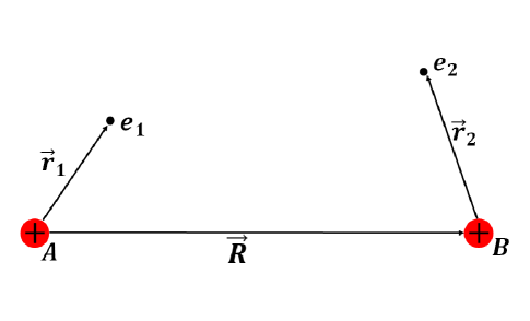
Figure 1: Two Rydberg atoms well separated from each other; each consists of a $+1$ nuclear core and a single, highly excited valence electron $e_{i}$. Here, the nuclear distance $R$ is greater than the LeRoy radius (see text) and thus much larger than either electron’s distance $r_{i}$ from its respective nuclear core.

Figure 1 schematically represents two such interacting Rydberg atoms: electron 1 is a distance $r_{1}$ from core $A$, and electron 2 is a distance $r_{2}$ from core $B$. In the long-range scenario, the nuclear distance $R$ is much larger than both $r_{1}$ and $r_{2}$. When the two nuclear cores are assumed to be fixed in space (no kinetic energy), then the interaction Hamiltonian is expressed in atomic units as:

$$\hat{H}=\hat{H}_{A}+\hat{H}_{B}+\hat{V}_{\rm int}\,\,,$$ (2)

where $\hat{H}_{i}$ contains the kinetic and potential energies of atom $i$ and $\hat{V}_{\rm int}$ is the Coulombic potential energy combinations of the two nuclei and the two electrons, given in atomic units as:

$$\hat{V}_{\rm int}=\dfrac{1}{R}-\dfrac{1}{|\vec{\boldsymbol{R}}+\vec{\boldsymbol{r}}_{2}|}-\dfrac{1}{|\vec{\boldsymbol{R}}-\vec{\boldsymbol{r}}_{1}|}+\dfrac{1}{|\vec{\boldsymbol{R}}+\vec{\boldsymbol{r}}_{2}-\vec{\boldsymbol{r}}_{1}|}\,\,.$$ (3)

II.1 Basis States

Given a non-relativistic Schrödinger equation, the fine-structure energy splitting is a result of the spin-orbit coupling between the total spin angular momentum of the dimer $\vec{\boldsymbol{S}}$ and the total orbital angular momentum of the dimer $\vec{\boldsymbol{L}}$. When nuclear rotation is neglected, Hund’s case (c) is the appropriate molecular basis where the good quantum numbers are the total angular momentum of the dimer $\vec{\boldsymbol{J}}=\vec{\boldsymbol{L}}+\vec{\boldsymbol{S}}$ and its projection $\Omega$ along the internuclear axis.

We adopt a typical approach and assume the dimer wave function to be a product of two atomic wave functions. Under the Born-Oppenheimer approximation, each atomic wave function is solely described by the quantum state of its valence electron 1 (2) about respective nucleus $A$ ($B$). In the coupled basis representation, each atom possesses total atomic angular momentum $\vec{\boldsymbol{j}}_{i}=\vec{\boldsymbol{\ell}}_{i}+\vec{\boldsymbol{s}}_{i}$, where $\vec{\boldsymbol{\ell}}_{i}$ is the orbital angular momentum of atom $i$ and $\vec{\boldsymbol{s}}_{i}$ is the spin angular momentum of atom $i$. The dimer wave functions are thus expressed as: $|1A\rangle\equiv|n_{1},\ell_{1},j_{1},m_{j_{1}}\rangle_{A}$ and $|2B\rangle\equiv|n_{2},\ell_{2},j_{2},\Omega-m_{j_{1}}\rangle_{B}$. Here $n_{i}$ is the principal quantum number of atom $i$, $\ell_{i}$ is the orbital angular momentum quantum number of atom $i$, and $m_{j_{i}}$ is the projection of the total atomic angular momentum $\vec{\boldsymbol{j}}_{i}$ of atom $i$ onto the internuclear axis (chosen in the $z$-direction for convenience).

For the interactions considered here, the fine-structure energies are too large for perturbation theory to be applicable. Thus, we directly diagonalize the interaction Hamiltonian at successive values of $R$ to compute electronic potential energy curves, as was done in Stanojevic et al. (2006, 2008). Such an approach has shown to be more successful at explaining experimental resonance features Farooqi et al. (2003) because it more accurately describes the intricate mixing of the electrons’ angular momentum characters ($\ell$-mixing).

To facilitate faster computational times, we exploit molecular symmetries to construct symmetrized molecular wave functions, as was done in Stanojevic et al. (2006, 2008); Samboy et al. (2011); Samboy and Côté (2011). Although the heteronuclear dimer does not possess the inversion symmetry of its homonuclear counterpart, the total wave function does remain anti-symmetric with respect to electron exchange. Therefore, as long as Equation (1) is satisfied, the properly symmetrized molecular wave function is given by:

$$|1A,2B;\Omega\rangle\sim\frac{1}{\sqrt{2}}\left(|1A\rangle|2B\rangle-|2B\rangle|1A\rangle\right).$$ (4)

For $\Omega=0$, reflection of the dimer through a plane containing the internuclear axis leads to wave functions that are either symmetric or anti-symmetric with respect to the reflection operator $\hat{\sigma}_{\nu}$. Furthermore, these wave functions have non-degenerate energy values and must be uniquely defined. We distinguish between the two based on how $\hat{\sigma}_{\nu}$ operates on (4):

$$|1A,2B;\Omega=0^{\pm}\rangle=\left(\dfrac{1\pm\hat{\sigma}_{\nu}}{\sqrt{2}}\right)|1A,2B;\Omega=0\rangle\,\,,$$ (5)

where $\hat{\sigma}_{\nu}$ behaves according to the following rules Bernath (2005); Brown and Carrington (2003):

$$\hat{\sigma}_{\nu}|\Lambda\rangle = (-1)^{\Lambda}|-\Lambda\rangle$$ (6)

$$\hat{\sigma}_{\nu}|S,M_{S}\rangle = (-1)^{S-M_{S}}|S,-M_{S}\rangle\,.$$ (7)

II.2 Basis sets

In general, any basis set (defined by $\Omega$) will consist of molecular states corresponding to those asymptotes with significant coupling to both the Rydberg-Rydberg asymptotic level being considered and to other nearby states. We gauge the relative interaction strengths of local asymptotes based on their contributions to the the $C_{6}\sim\dfrac{(\langle\phi_{1}|r|\phi_{2}\rangle\langle\phi_{3}|r|\phi_{4}\rangle)^{2}}{(E_{1}+E_{3})-(E_{2}+E_{4})}$ (dipole-dipole) and $C_{5}\sim\langle\phi_{1}|r^{2}|\phi_{2}\rangle\langle\phi_{3}|r^{2}|\phi_{4}\rangle$ (quadrupole-quadrupole) coefficients of the molecular Rydberg state being considered. In these expressions, each $E_{i}$ is the asymptotic energy of atom $i$ in state $\phi_{i}$ and $\langle\phi_{i}|r^{k}|\phi_{j}\rangle$ is the radial matrix element between atoms $i$ and $j$.

As mentioned before, the $C_{i}$ coefficients (perturbation theory) are not sufficient to properly describe the long-range Rydberg-Rydberg interaction picture detailed in this work; however, such analysis does accurately assess which asymptotes provide strong coupling and which do not. For example, if we consider the $70^{(\rm K)}s+70^{(\rm Rb)}s$ Rydberg level the largest contribution to the $C_{6}$ coefficient comes from the $69^{(\rm K)}p+70^{(\rm Rb)}p$ state ($8.89317\times 10^{14}$), while the largest contribution to the $C_{5}$ coefficient comes from the $67^{(\rm K)}d+69^{(\rm Rb)}d$ state ($3.8039\times 10^{15}$) and the $68^{(\rm K)}d+70^{(\rm Rb)}d$ state ($2.4682\times 10^{15}$). To provide some contrast, the contribution of the $71^{(\rm K)}p+71^{(\rm Rb)}p$ state to the $C_{6}$ coefficient is $2.51707\times 10^{9}$, while the contribution of the $72^{(\rm K)}d+72^{(\rm Rb)}d$ state to the $C_{5}$ coefficient is $3.80343\times 10^{11}$. Since the contributions of these states are 4 or 5 orders of magnitude smaller, they are not included in the basis.

To construct a more complete basis set, we examine asymptotes in the vicinity $(\sim\pm 20$ GHz) of the molecular Rydberg level being considered and we find in Table 1 that the dipole strength between two atomic Rydberg states decays rapidly with the relative difference in their principal quantum numbers: $\Delta n\equiv|n_{1}-n_{2}|$. Note: This table details specific results for transitions from rubidium in the $70s$ state and from potassium in the $70s$ state, but similar behaviors are found for transitions from any excited $n\ell$ Rydberg state. Due to the sharp decline in the coupling strengths, we only consider nearby asymptotic levels whose two constituent atoms have $n_{i}$ values in the range $(n-3)\leq n_{i}\leq(n+3)$, where $n$ is the principal quantum number of the excited Rydberg state for each atom ($n=70$ for all tabulated results in this paper).

Table 1: Dipole matrix elements for atomic transitions from (left) Rb $70s$ and (right) K $70s$. We highlight the two largest elements for each atomic species and note the rapid decrease in coupling strength as $\Delta n=|n_{1}-n_{2}|$ increases.

Rubidium			Potassium
$\langle 70s|r|74p_{3/2}\rangle$	$=$	94.064	$\langle 70s|r|74p_{3/2}\rangle$	$=$	87.093
$\langle 70s|r|73p_{3/2}\rangle$	$=$	-144.19	$\langle 70s|r|73p_{3/2}\rangle$	$=$	-134.41
$\langle 70s|r|72p_{3/2}\rangle$	$=$	258.08	$\langle 70s|r|72p_{3/2}\rangle$	$=$	243.23
$\langle 70s|r|71p_{3/2}\rangle$	$=$	-639.57	$\langle 70s|r|71p_{3/2}\rangle$	$=$	-616.30
$\langle 70s|r|70p_{3/2}\rangle$	$=$	5081.6	$\langle 70s|r|70p_{3/2}\rangle$	$=$	5353.1
$\langle 70s|r|69p_{3/2}\rangle$	$=$	4807.8	$\langle 70s|r|69p_{3/2}\rangle$	$=$	4810.7
$\langle 70s|r|68p_{3/2}\rangle$	$=$	-649.29	$\langle 70s|r|68p_{3/2}\rangle$	$=$	-696.92
$\langle 70s|r|67p_{3/2}\rangle$	$=$	262.07	$\langle 70s|r|67p_{3/2}\rangle$	$=$	285.92
$\langle 70s|r|66p_{3/2}\rangle$	$=$	-144.50	$\langle 70s|r|66p_{3/2}\rangle$	$=$	-158.83

Table 2 lists the relevant molecular levels near the $70s+70s$ asymptote and the $70p+70p$ asymptote; the properly symmetrized states corresponding to these molecular levels comprise the appropriate basis sets.

Table 2: Molecular asymptotes included in the basis sets for the long-range interactions between rubidium and potassium: (left) each atom excited to the $70s$ Rydberg state, and (right) each atom excited to the $70p$ Rydberg state.

K$(70s)$-Rb$(70s)$	K$(70p)$-Rb$(70p)$
$68^{(\rm K)}d+70^{(\rm Rb)}s$	$67^{(\rm K)}f+71^{(\rm Rb)}p$
$69^{(\rm K)}s+69^{(\rm Rb)}d$	$68^{(\rm K)}f+70^{(\rm Rb)}p$
$68^{(\rm K)}p+71^{(\rm Rb)}p$	$68^{(\rm K)}d+69^{(\rm Rb)}d$
$69^{(\rm K)}p+70^{(\rm Rb)}p$	$69^{(\rm K)}s+70^{(\rm Rb)}d$
$69^{(\rm K)}s+71^{(\rm Rb)}s$	$67^{(\rm K)}d+72^{(\rm Rb)}s$
$70^{(\rm K)}s+70^{(\rm Rb)}s$	$69^{(\rm K)}d+70^{(\rm Rb)}s$
$68^{(\rm K)}d+69^{(\rm Rb)}d$	$68^{(\rm K)}d+71^{(\rm Rb)}s$
	$69^{(\rm K)}p+71^{(\rm Rb)}p$
	$70^{(\rm K)}p+70^{(\rm Rb)}p$
	$69^{(\rm K)}s+72^{(\rm Rb)}s$
	$70^{(\rm K)}s+71^{(\rm Rb)}s$
	$67^{(\rm K)}f+69^{(\rm Rb)}f$
	$68^{(\rm K)}f+68^{(\rm Rb)}f$

II.3 Interaction Hamiltonian

Under the Born-Oppenheimer approximation, diagonalization of the interaction Hamiltonian (Eq. (2)) results in a set of electronic energies with regard to a fixed nuclear separation $R$. A complete set of electronic energy curves can be calculated by diagonalizing a unique Hamiltonian matrix at varying values of $R$.

A convenient approach for long-range Rydberg investigations is to express the Coulombic potential energy expression (Eq. (3)) as a multipole expansion in inverse powers of $R$ Rose (1958); Buehler and Hirschfelder (1951); Carlson and Rushbrooke (1950); the expansion is further simplified if we assume $\vec{\boldsymbol{R}}$ lies along a $z-$axis, common to both Rydberg atoms Fontana (1961):

$$\hat{V}_{\rm int}\equiv V_{L}(R) ={\displaystyle\sum_{L=0}^{\infty}}(-1)^{L}\dfrac{4\pi}{R^{2L+1}(2L+1)}r_{1}^{L}r_{2}^{L}$$

$$\times{\displaystyle\sum_{m=-L}^{L}}B_{2L}^{L+m}\,Y_{L}^{m}(\hat{\boldsymbol{r}}_{1})\,Y_{L}^{-m}(\hat{\boldsymbol{r}}_{2})\,\,.$$ (8)

Here, $B_{n}^{k}\equiv\frac{n!}{k!(n-k)!}$ is the binomial coefficient, $Y_{L}^{m}(\hat{\boldsymbol{r}}_{i})$ is a spherical harmonic describing the angular position of electron $i$ with position $\vec{\boldsymbol{r}}_{i}$ from its nuclear center, $L$ labels the ($2^{L}$) multi-pole moment ($L=1$ for dipolar, $L=2$ for quadrupolar, etc.), and $R$ is the internuclear distance. The advantage to such an expansion is that the expression can be truncated such that only meaningful terms are kept; this significantly reduces computation time.

When the Hamiltonian is diagonalized, the expectation value of each term in the energy expansion is proportional to $\dfrac{\langle r_{1}^{L}\rangle\langle r_{2}^{L}\rangle}{R^{2L+1}}$; for Rydberg atoms, each radial element scales as $\langle r^{L}\rangle\sim n^{2L}$Gallagher (1994). Thus, dipole-dipole interactions scale as $\sim\dfrac{n^{4}}{R^{3}}$, quadrupole-quadrupole interactions scale as $\sim\dfrac{n^{8}}{R^{5}}$ and so on. For the internuclear spacings considered here, $R\approx n^{5/2}$, so the dipole-dipole coupling strength is $\sim n^{-7/2}$ and the quadrupole-quadrupole coupling strength is $\sim n^{-9/2}$.

Typically, dipole-dipole interactions dominate the long-range Rydberg-Rydberg interactions, but it has been shown Stanojevic et al. (2008); Schwettmann et al. (2006) that quadrupole-quadrupole couplings can also be significant to the interaction picture. To date, octupole-octupole interactions have not been shown to be relevant in long-range Rydberg interactions, so we do not consider them here. Based on the scaling relations shown above, such a term would be a factor of $n^{-1}$ less than the quadrupole-quadrupole term and a factor of $n^{-2}$ less than the dipole-dipole term.

Because the molecular basis states are linear combinations of atomic states determined through symmetry considerations (see Eq. (4)), each matrix element in the interaction Hamiltonian is actually a combination of multiple interaction terms:

$$\langle 1A,2B;\Omega| \hat{H}|3A,4B;\Omega\rangle\sim$$

$$\langle 1A,2B|\hat{H}|3A,4B\rangle$$

$$- \langle 1A,2B|\hat{H}|4A,3B\rangle$$ (9)

$$- \langle 2A,1B|\hat{H}|3A;4B\rangle$$

$$+ \langle 2A,1B|\hat{H}|4A;3B\rangle\;.$$

For the $\Omega=0$ case, equation (5) is also applied, resulting in additional terms. Since the normalization factor varies with state definitions and symmetry considerations, it is not stated explicitly in (II.3). Normalization factors are included in calculations, however. In this notation,
$|1A,2B\rangle=|n_{1},\ell_{1},j_{1},m_{j_{1}}\rangle_{A}|n_{2},\ell_{2},j_{2},\Omega-m_{j_{1}}\rangle_{B}$, and so on.

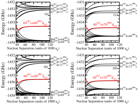
Figure 2: (Color online) Long-range potential energy curves corresponding to the interactions between one rubidium atom and one potassium atom excited to the same state. The curves in panel (a) correspond to the $\Omega=0^{+}$ symmetry with both atoms excited to the $70s$ state, the curves in panel (b) correspond to the $\Omega=0^{-}$ symmetry with both atoms excited to the $70s$ state, the curves in panel (c) correspond to the $\Omega=0^{+}$ symmetry with both atoms excited to the $70p$ state and the curves in panel (d) correspond to the $\Omega=0^{-}$ symmetry with both atoms excited to the $70p$ state. We highlight the potential energy wells in red and label their respective asymptotic states.

An analytical expression for any given term in the matrix element is found to be:

$$\langle 1A,2B|V_{L}(R)|3A,4B\rangle=$$

$$(-1)^{L-1-\Omega+j_{\rm tot}}\sqrt{\hat{\ell}_{1}\hat{\ell}_{2}\hat{\ell}_{3}\hat{\ell}_{4}\hat{j}_{1}\hat{j}_{2}\hat{j}_{3}\hat{j}_{4}}\;\dfrac{\mathcal{R}_{13,A}^{L}\;\mathcal{R}_{24,B}^{L}}{R^{2L+1}}$$

$$\times\left(\begin{array}[]{ccc}\ell_{1}&L&\ell_{3}\\ 0&0&0\\ \end{array}\right)\left(\begin{array}[]{ccc}\ell_{2}&L&\ell_{4}\\ 0&0&0\\ \end{array}\right)$$ (14)

$$\times\left\{\begin{array}[]{ccc}j_{1}&L&j_{3}\\ \ell_{3}&\frac{1}{2}&\ell_{1}\\ \end{array}\right\}\left\{\begin{array}[]{ccc}j_{2}&L&j_{4}\\ \ell_{4}&\frac{1}{2}&\ell_{2}\\ \end{array}\right\}$$ (19)

$$\times{\displaystyle\sum_{m=-L}^{L}}B_{2L}^{L+m}\left(\begin{array}[]{ccc}j_{1}&L&j_{3}\\ -m_{j_{1}}&m&m_{j_{3}}\\ \end{array}\right)$$ (22)

$$\times\left(\begin{array}[]{ccc}j_{2}&L&j_{4}\\ -m_{j_{2}}&-m&m_{j_{4}}\\ \end{array}\right)\,\,,$$ (25)

where $j_{\rm tot}=j_{1}+j_{2}+j_{3}+j_{4}$, $\hat{\ell}_{i}=2\ell_{i}+1$, $\hat{j}_{i}=2j_{i}+1$, and $\mathcal{R}_{ij,Q}^{L}=\langle i|r^{L}|j\rangle_{Q}$ is the radial matrix element of atom $Q$. The $(\cdots)$ expressions represent Wigner-$3j$ symbols, and the $\{\cdots\}$ represent Wigner-$6j$ symbols.

The diagonal elements, i.e. $|1A,2B\rangle~{}=~{}|3A,4B\rangle$ are given by:

$$\langle 1A,2B;\Omega|\hat{H}| 1A,2B;\Omega\rangle=$$

$$\langle 1A,2B;\Omega|V_{L}(R)|1A,2B;\Omega\rangle$$

$$+ \,\,E_{1A}+E_{2B}\,,$$ (26)

where $\langle 1A,2B;\Omega|V_{L}(R)|1A,2B;\Omega\rangle$ follows (II.3) and (II.3), and each $E_{iQ}$ is the asymptotic energy of the atomic Rydberg state $|n_{i},\ell_{i},j_{i},m_{j_{i}}\rangle_{Q}$:

$$E_{iQ}=-\dfrac{1}{2(n_{iQ}-\delta_{\ell_{i}Q})}\,\,.$$ (27)

In this expression, $n_{iQ}$ is the principal quantum number of atom $Q$ and $\delta_{\ell_{i}Q}$ is the quantum defect for atom $Q$ (values given in Gallagher (1994); Li et al. (2003); Han et al. (2006)).

III Interaction Curves

After investigating all possible $\Omega$-symmetries for the $70s+70s$ and $70p+70p$ excitations of rubidium and potassium, we found that in both cases the $\Omega=0^{+}$ and the $\Omega=0^{-}$ symmetries resulted in potential wells capable of supporting bound states. In Figure 2, we plot the interaction energies for these four cases against the Bohr radius ($a_{0}$) and highlight the resulting potential wells in red; we also label the wells’ corresponding asymptotic energy levels.

For all four of these wells, we explored scaling relations, composition, and stability. We provide a visual example in Figure 3(a), where the potential well corresponding to the $\Omega=0^{+}$ symmetry for both atoms excited to the $70s$ state is isolated. This well is $\sim 600$ MHz deep and supports $\sim 630$ bound vibrational states. In Table 4, we present the first few bound state vibrational energies (as measured from the bottom of the well) for all four wells, as well as the classical turning points, indicating the large size of these dimer states. Given that the equilibrium separation $R_{e}$ for all four wells is between 41,000 $a_{0}$ and 46,000 $a_{0}$ $(\sim 2.25$ $\mu$m), these bound states are very extended, consistent with the macrodimer classification.

The inset of Figure 3(a) shows that the deepest part of the wells can be well-modeled as a harmonic potential; the first few bound levels for each well are consistently spaced (see Table 4). The bound energies and corresponding wave functions were calculated using the mapped Fourier Grid Method Kokoouline et al. (1999) for each potential well individually.

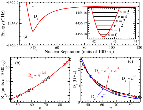
Figure 3: (Color online) (a) Long-range potential energy curves corresponding to the $\Omega=0^{+}$ symmetry interactions of one potassium Rydberg atom and one rubidium Rydberg atom; both atoms have been excited to the 70$s$ state. We note the existence of a $\sim$ 600 MHz deep well (associated with the $69^{(\rm K)}s+69^{(\rm Rb)}d_{5/2}$ asymptotic level), capable of supporting many bound states. We explicitly label the equilibrium separation $R_{e}$ and the dissociation energy $D_{e}$. Inset: Zoom of the deepest part of the well, showing the first few bound vibrational levels; corresponding energies and classical turning points are given in Table 4. (b) Scaling relations for the equilibrium separation $R_{e}$ vs. principal quantum number $n$: $R_{e}\sim n^{12/5}$. (c) Scaling relations for the dissociation energy $D_{e}$ vs. principal quantum number $n$. Three different results (see text) are shown: $D_{e}\sim n^{-4}$ (blue) gives poor agreement, $D_{e}\sim n^{-3}$ (black-dashed) gives good agreement, but $D_{e}\sim n^{-3}+n^{-4}$ (red) gives the best agreement.

III.1 Scaling Relations

The dissociation energy $D_{e}$ and the equilibrium separation $R_{e}$ for the potential wells were were calculated for various values of the principal quantum number $n$. In panels (b) and (c) of Figure 3, we show the results for the $\Omega=0^{+}$ symmetry with both atoms excited to the $70s$ state. In panel (b), we see that the equilibrium separation scales as $n^{12/5}$, and in panel (c), we present different “best-fit” curves corresponding to different values of $n$-scaling for the dissociation energy. For pure dipole-dipole coupling, one would expect the dissociation energy to scale as the energy difference between energy levels ($n^{-3}$ for Rydberg atoms Gallagher (1994)). We see that this result gives pretty good agreement, but the results suggest that $D_{e}$ actually scales as $\sim n^{-4}+n^{-3}$. Although it gives poor agreement, we also include the curve of $n^{-4}$ for completeness. In Table 3, we present the scaling results for all four of the potential wells identified in Figure 2. We note that the scaling results obtained here for $R_{e}$ and $D_{e}$ are consistent with the results for homonuclear macrodimers, presented in Samboy and Côté (2011). A thorough derivation for these scaling relations was also performed in that work; we do not republish them here.

Table 3: $n$-scaling relations for the equilibrium separation $R_{e}$ and the dissociation energy $D_{e}$ for the four potential wells discussed in this work (see Figure 2). Both results are consistent with previous work regarding homonuclear macrodimers (see text).

Threshold energy (well)	Symmetry	$R_{e}$ scaling	$D_{e}$ scaling
$69^{(\rm K)}s+69^{(\rm Rb)}d_{5/2}$	$\Omega=0^{+}$	$n^{2.4}$ ($n^{12/5}$)	$n^{-3}+n^{-4}$
$69^{(\rm K)}s+69^{(\rm Rb)}d_{5/2}$	$\Omega=0^{-}$	$n^{2.4}$ ($n^{12/5}$)	$n^{-3}+n^{-4}$
$69^{(\rm K)}s+70^{(\rm Rb)}d_{5/2}$	$\Omega=0^{+}$	$n^{2.3}$	$n^{-3}+n^{-4}$
$69^{(\rm K)}s+70^{(\rm Rb)}d_{5/2}$	$\Omega=0^{-}$	$n^{2.3}$	$n^{-3}+n^{-4}$

III.2 Well composition and stability

Due to the electronic $\ell$-mixing, each potential energy curve $U_{\lambda}(R)$ is described by an electronic wave function $|\chi_{\lambda}(R)\rangle$, which itself is a superposition of the asymptotic molecular wave functions (4):

$$|\chi_{\lambda}(R)\rangle={\displaystyle\sum_{j}c_{j}^{(\lambda)}(R)}|j\rangle\,\,.$$ (28)

The exact amount of mixing varies with $R$, and is completely described by the $c_{j}^{(\lambda)}(R)$ coefficients: the eigenvectors after diagonalization. The $|j\rangle$ are the corresponding symmetrized basis states $|1A,2B;\Omega\rangle$, defined earlier (4). As an example of the $R$-dependence of the mixing, in Figure 4(b) we illustrate the composition of the potential well highlighted in Figures 3(a) and 4(a). This potential curve corresponds to the $69^{(\rm K)}s+69^{(\rm Rb)}d_{5/2}$ asymptote.

As would be expected, this well is mainly composed of the $69^{(\rm K)}s+69^{(\rm Rb)}d_{5/2}$ state. However, in the region of the actual well, we also see significant contributions from the $69^{(\rm K)}s+69^{(\rm Rb)}d_{3/2}$ directly below the well, and even from some deeper $nd+n^{\prime}d$ states. In Figure 4(a), we highlight and label the four states most relevant to $\ell$-mixing; the corresponding probabilities $\left|c_{j}(R)\right|^{2}$ of these states are plotted against $R$ in Figure 4(b) to explicitly describe the $R$-dependence. We note that the effects from $\ell$-mixing cease when the nuclear separation is about 60,000 $a_{0}$. This is obvious by the probability coefficient of the $69^{(\rm K)}s+69^{(\rm Rb)}d_{5/2}$ state approaching one, while all other coefficients approach zero. Also of note is the switch in probabilities of the $69^{(\rm K)}s+69^{(\rm Rb)}d_{5/2}$ and $69^{(\rm K)}s+69^{(\rm Rb)}d_{3/2}$ states between $\sim$ 55,000 $a_{0}$ and $\sim$ 57,000 $a_{0}$. Although perhaps not visually obvious in the Figure 4(a) panel, these two curves do appear to experience an avoided crossing in this general vicinity: one can observe a slight deviation in the line shapes of these two curves as they meet. Such a crossing would be consistent with the behavior of the probabilities.

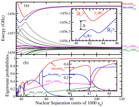
Figure 4: (Color Online) (a) $\Omega=0^{+}$ potential energy curves describing the interactions between one potassium Rydberg atom and one rubidium Rydberg atom: both atoms have been excited to the $70s$ state. We highlight those curves corresponding to the electronic states that contribute the most to the formation of the well (see text). Inset: Zoom of the region near the avoided crossing, indicating the relevant features of the Landau-Zener treatment: $\Delta$ is the energy gap between the adiabatic energies $\epsilon_{1}$ and $\epsilon_{2}$ at closest approach; these adiabatic energies correspond to the two adiabatic states $|\chi_{1}\rangle$ and $|\chi_{2}\rangle$ at the avoided crossing. (b) Probabilities $\left|c_{j}(R)\right|^{2}$ of the electronic basis states $|j\rangle$ most responsible for the formation of the well (see text). After $\sim$ 60,000 $a_{0}$, the $\ell$-mixing is negligible: the probability coefficient corresponding to $69^{\rm(K)}s+^{(\rm Rb)}70d_{5/2}$ approaches one (see dashed line) and all other probability coefficients decay to zero. Inset: Zoom of the region near the avoided crossing. All panels use the same labeling/color scheme.

For potential energy wells formed via some avoided crossing between curves, predissociation of bound energy levels can be a concern. In general, avoided crossings can lead to predissociation if the (meta-)stable state has strong coupling to the unstable state below it. From the eigenvector plot in Figure 4(b), we see that there is significant coupling between the potential well and the curves that lie below it. Therefore, the long-term stability of these wells could be compromised.

Table 4: Energies of the deepest bound levels (measured from the bottom of the well), classical turning points ($R_{1}$, $R_{2}$), and dimer lifetimes $\tau$ (see text) for the four potential wells identified in Figure 2.

Excited Rydberg pair	spThreshold energy (well)sp	Symmetry	$v$	Energy (MHz)	$R_{1}$ (a.u.)	$R_{2}$ (a.u.)	$\tau$ (s)
$70^{(\rm K)}s+70^{(\rm Rb)}s$	$69^{(\rm K)}s+69^{(\rm Rb)}d_{5/2}$	$\Omega=0^{+}$	0	002.2240	42 175	42 783	$\infty$
			1	006.6490	42 175	42 784	$\infty$
			2	010.9194	42 095	42 891	$\infty$
			3	015.0636	42 031	42 985	$\infty$
			4	019.0879	41 976	43 070	$\infty$
			5	023.0177	41 926	43 149	$\infty$
			$\vdots$	$\vdots$	$\vdots$	$\vdots$	$\vdots$
			627	591.9279	37 967	226 597	$\infty$
$70^{(\rm K)}s+70^{(\rm Rb)}s$	$69^{(\rm K)}s+69^{(\rm Rb)}d_{5/2}$	$\Omega=0^{-}$	0	001.7120	41 591	41 983	$\infty$
			1	005.1375	41 456	42 145	$\infty$
			2	008.5053	41 366	42 260	$\infty$
			3	011.8269	41 292	42 360	$\infty$
			4	015.0967	41 232	42 447	$\infty$
			5	018.3146	41 177	42 527	$\infty$
			$\vdots$	$\vdots$	$\vdots$	$\vdots$	$\vdots$
			608	564.7000	37 067	157 474	$\infty$
$70^{(\rm K)}p+70^{(\rm Rb)}p$	$69^{(\rm K)}s+70^{(\rm Rb)}d_{5/2}$	$\Omega=0^{+}$	0	001.3422	45 088	45 535	$\infty$
			1	003.9897	44 937	45 718	$\infty$
			2	006.5859	44 834	45 854	$\infty$
			3	009.1309	44 750	45 970	$\infty$
			4	011.6247	44 681	46 073	$\infty$
			5	014.0752	44 620	46 169	$\infty$
			$\vdots$	$\vdots$	$\vdots$	$\vdots$	$\vdots$
			470	335.6738	40 716	181 441	$\infty$
$70^{(\rm K)}p+70^{(\rm Rb)}p$	$69^{(\rm K)}s+70^{(\rm Rb)}d_{5/2}$	$\Omega=0^{-}$	0	001.3682	45 072	45 512	$\infty$
			1	004.0782	44 921	45 696	$\infty$
			2	006.7330	44 821	45 832	$\infty$
			3	009.3245	44 739	45 947	$\infty$
			4	011.8687	44 670	46 050	$\infty$
			5	014.3575	44 608	46 147	$\infty$
			$\vdots$	$\vdots$	$\vdots$	$\vdots$	$\vdots$
			473	337.7708	40 746	158 929	$\infty$

For curves that are less intricate, a simple Landau-Zener Landau and Lifshitz (1997); Zener (1932) treatment would be desirable. However, such an approach depends on detailed knowledge of the diabatic crossing behavior, including which diabatic states actually correspond to the crossing potential energy curves; for the complicated curve mixings that we demonstrate, defining these diabatic states becomes difficult. Instead, we adopt the approach taken by Clark Clark (1979), in which the parameters defining the Landau-Zener probability are obtained from the adiabatic $P$-matrix coupling. Specifically, the $P$-matrix is defined through the off-diagonal derivative of the interaction potential between the crossing states:

$$P_{12}(R)=\dfrac{\langle\chi_{1}|(\partial/\partial R)V(R)|\chi_{2}\rangle}{\left(\varepsilon_{1}(R)-\varepsilon_{2}(R)\right)}\,\,.$$ (29)

Here, $\varepsilon_{i}(R)$ is the energy value of the adiabatic potential curve described by state $|\chi_{i}\rangle$, and $V(R)$ is defined by equation (II.3). As the nuclear separation is varied, the value of the $P$-matrix peaks when the adiabatic curves are at their closest approach (corresponding to $\varepsilon_{1}(R)-\varepsilon_{2}(R)$ being a minimum). Clark showed that by fitting the $P$-matrix to a Lorentzian function, the probability $P_{LZ}$ to make a non-adiabatic transition from the electronic state $|\chi_{1}\rangle$ to the electronic state $|\chi_{2}\rangle$ is given by:

$$P_{LZ}=\exp{\left(-\dfrac{2\pi}{v}\dfrac{\Delta}{8\,P_{\rm max}}\right)}\,\,,$$ (30)

where $v$ is the relative velocity of the two nuclei determined from the bound levels of the molecule, $\Delta$ is the energy gap between the two adiabatic curves at closest approach, and $P_{\rm max}$ is the peak value of the $P$-matrix. The inset of Figure 4(a) shows a close-up of the avoided crossing between the $|\chi_{1}\rangle\equiv 69^{(\rm K)}s+69^{(\rm Rb)}d_{5/2}$ and $|\chi_{2}\rangle\equiv 69^{(\rm K)}s+69^{(\rm Rb)}d_{3/2}$ electronic states; the energy gap $\Delta$ is also indicated.

Since $P_{LZ}$ represents the likelihood of transitioning from $|\chi_{1}\rangle$ to $|\chi_{2}\rangle$ (and thus predissociating into two free atoms), then $1-P_{LZ}$ is the probability that the macrodimer will remain in $|\chi_{1}\rangle$ and not predissociate. We match this probability to an exponential decay over the time $t$ for a full oscillation inside the well: $1-P_{LZ}=e^{-t/\tau}$ and find $\tau$, the “lifetime” of the dimer; the results are summarized in Table 4.

Our calculations show that all of the bound states have near-zero $P_{LZ}$ values and thus near-infinite lifetimes. Although there is strong coupling between the well and the states below it, the energy gap between the well and the lower curves is too large for dissociation to occur. In addition, the oscillation speeds of the dimers are too slow for diabatic transitions. We therefore conclude that these dimers are stable with respect to predissociation and so their lifetime is limited only by the Ryberg atoms themselves ($t_{\rm Ryd}\sim 700$ $\mu$s for $n=70$) Beterov et al. (2009).

IV Conclusions

In this paper, we investigated the long-range interactions between rubidium and potassium, where both atoms are excited to high-$n$ Rydberg states. We explored all possible $\Omega$-symmetries for both atoms being excited to the $70s$ state and the $70p$ state. Our calculations showed that due to the effects of electronic $\ell$-mixing, the potential energy curves describing these interactions are intricate and complicated, particularly when the nuclear separations are in the 40,000 $a_{0}$ - 60,000 $a_{0}$ range. In addition, when both atoms are excited to either the $70s$ state or the $70p$ state, both the $\Omega=0^{+}$ symmetry interactions and the $\Omega=0^{-}$ symmetry interactions result in potential wells capable of supporting many bound states. We analyzed these wells in detail, calculating the bound vibrational levels, the stability of these levels, and various $n$-scaling relations.

Given the interest in photoassociation experiments between different alkali species, these results could be useful to further ultracold experiments, quantum chemistry calculations, and/or quantum information research. Furthermore, it might be possible to exploit the $\ell$-mixing for application to “dressed” Rydberg states Johnson and Rolston (2010); Helmrich et al. (2016).

References

- Gallagher (1994) T. Gallagher, Rydberg Atoms (Cambridge University Press, Cambridge, United Kingdom, 1994).
- Anderson et al. (1998a) W. R. Anderson, J. R. Veale, and T. F. Gallagher, Phys. Rev. Lett. 80, 249 (1998a).
- Mourachko et al. (1998) I. Mourachko, D. Comparat, F. de Tomasi, A. Fioretti, P. Nosbaum, V. M. Akulin, and P. Pillet, Phys. Rev. Lett. 80, 253 (1998).
- Farooqi et al. (2003) S. M. Farooqi, D. Tong, S. Krishnan, J. Stanojevic, Y. P. Zhang, J. R. Ensher, A. S. Estrin, C. Boisseau, R. Côté, E. E. Eyler, and P. L. Gould, Phys. Rev. Lett. 91, 183002 (2003).
- Overstreet et al. (2007) K. R. Overstreet, A. Schwettmann, J. Tallant, and J. P. Shaffer, Phys. Rev. A 76, 011403 (2007).
- Greene et al. (2000) C. H. Greene, A. S. Dickinson, and H. R. Sadeghpour, Phys. Rev. Lett. 85, 2458 (2000).
- Bendowsky et al. (2009) V. Bendowsky, B. Butscher, J. Nipper, J. P. Shaffer, R. Löw, and T. Pfau, Nature 458, 1005 (2009).
- Boisseau et al. (2002) C. Boisseau, I. Simbotin, and R. Côté, Phys. Rev. Lett. 88, 133004 (2002).
- Samboy et al. (2011) N. Samboy, J. Stanojevic, and R. Côté, Phys. Rev. A 83, 050501 (2011).
- Samboy and Côté (2011) N. Samboy and R. Côté, Journal of Physics B: Atomic, Molecular and Optical Physics 44, 184006 (2011).
- Overstreet et al. (2009) K. R. Overstreet, A. Schwettmann, J. Tallant, D. Booth, and J. P. Shaffer, Nature Physics 5, 581 (2009).
- Lukin et al. (2001) M. D. Lukin, M. Fleischhauer, R. Cote, L. M. Duan, D. Jaksch, J. I. Cirac, and P. Zoller, Phys. Rev. Lett. 87, 037901 (2001).
- Saffman et al. (2010) M. Saffman, T. G. Walker, and K. Mølmer, Rev. Mod. Phys. 82, 2313 (2010).
- Marcassa and Shaffer (2014) L. G. Marcassa and J. P. Shaffer (Academic Press, 2014) pp. 47 – 133.
- Rittenhouse et al. (2011) S. T. Rittenhouse, M. Mayle, P. Schmelcher, and H. R. Sadeghpour, Journal of Physics B: Atomic, Molecular and Optical Physics 44, 184005 (2011).
- Rittenhouse and Sadeghpour (2010) S. T. Rittenhouse and H. R. Sadeghpour, Phys. Rev. Lett. 104, 243002 (2010).
- Liu and Rost (2006) I. C. H. Liu and J. M. Rost, Eur. Phys. J. D 40, 65 (2006).
- Liu et al. (2009) I. C. H. Liu, J. Stanojevic, and J. M. Rost, Phys. Rev. Lett. 102, 173001 (2009).
- Samboy and Côté (2013) N. Samboy and R. Côté, Phys. Rev. A 87, 032512 (2013).
- Kiffner et al. (2013) M. Kiffner, W. Li, and D. Jaksch, Phys. Rev. Lett. 111, 233003 (2013).
- Kiffner et al. (2014) M. Kiffner, M. Huo, W. Li, and D. Jaksch, Phys. Rev. A 89, 052717 (2014).
- Vaillant et al. (2012) C. L. Vaillant, M. P. A. Jones, and R. M. Potvliege, Journal of Physics B: Atomic, Molecular and Optical Physics 45, 135004 (2012).
- Ye et al. (2013) S. Ye, X. Zhang, T. C. Killian, F. B. Dunning, M. Hiller, S. Yoshida, S. Nagele, and J. Burgdörfer, Phys. Rev. A 88, 043430 (2013).
- Camargo et al. (2016) F. Camargo, J. D. Whalen, R. Ding, H. R. Sadeghpour, S. Yoshida, J. Burgdörfer, F. B. Dunning, and T. C. Killian, Phys. Rev. A 93, 022702 (2016).
- Banerjee et al. (2013a) J. Banerjee, D. Rahmlow, R. Carollo, M. Bellos, E. E. Eyler, P. L. Gould, and W. C. Stwalley, The Journal of Chemical Physics 139, 174316 (2013a), http://dx.doi.org/10.1063/1.4826653.
- Banerjee et al. (2013b) J. Banerjee, D. Rahmlow, R. Carollo, M. Bellos, E. E. Eyler, P. L. Gould, and W. C. Stwalley, The Journal of Chemical Physics 138, 164302 (2013b), http://dx.doi.org/10.1063/1.4801441.
- Calarco et al. (2000) T. Calarco, H. Briegel, D. Jaksch, J. Cirac, and P. Zoller, J. Mod. Opt. 47, 2137 (2000).
- Vollbrecht et al. (2004) K. G. H. Vollbrecht, E. Solano, and J. I. Cirac, Phys. Rev. Lett. 93, 220502 (2004).
- Anderson et al. (1998b) W. R. Anderson, J. R. Veale, and T. F. Gallagher, Phys. Rev. Lett. 80, 249 (1998b).
- LeRoy (1974) R. J. LeRoy, Can. J. Phys. 52, 246 (1974).
- Stanojevic et al. (2006) J. Stanojevic, R. Côté, D. Tong, S. Farooqi, E. Eyler, and P. Gould, Eur. Phys. J. D 40, 3 (2006).
- Stanojevic et al. (2008) J. Stanojevic, R. Côté, D. Tong, E. E. Eyler, and P. L. Gould, Phys. Rev. A 78, 052709 (2008).
- Bernath (2005) P. Bernath, Spectra of Atoms and Molecules (Oxford University Press, New York, New York, 2005).
- Brown and Carrington (2003) J. Brown and A. Carrington, Rotational Spectroscopy of Diatomic Molecules (Cambridge University Press, Cambridge, United Kingdom, 2003).
- Rose (1958) M. E. Rose, J. Phys. Math 37, 215 (1958).
- Buehler and Hirschfelder (1951) R. J. Buehler and J. O. Hirschfelder, Phys. Rev. 83, 628 (1951).
- Carlson and Rushbrooke (1950) B. C. Carlson and G. S. Rushbrooke, Mathematical Proceedings of the Cambridge Philosophical Society 46, 626 (1950).
- Fontana (1961) P. R. Fontana, Phys. Rev. 123, 1865 (1961).
- Schwettmann et al. (2006) A. Schwettmann, J. Crawford, K. R. Overstreet, and J. P. Shaffer, Phys. Rev. A 74, 020701 (2006).
- Li et al. (2003) W. Li, I. Mourachko, M. W. Noel, and T. F. Gallagher, Phys. Rev. A 67, 052502 (2003).
- Han et al. (2006) J. Han, Y. Jamil, D. V. L. Norum, P. J. Tanner, and T. F. Gallagher, Phys. Rev. A 74, 054502 (2006).
- Kokoouline et al. (1999) V. Kokoouline, O. Dulieu, R. Kosloff, and F. Masnou-Seeuws, Journal of Chemical Physics 110, 9865 (1999).
- Landau and Lifshitz (1997) L. Landau and E. Lifshitz, Quantum Mechanics (Non-relativistic Theory), Third Edition (Pergamon Press Ltd., Oxford, Great Britain, 1997).
- Zener (1932) C. Zener, Proc. R. Lond. A 137, 696 (1932).
- Clark (1979) C. W. Clark, Physics Letters 70A, 295 (1979).
- Beterov et al. (2009) I. I. Beterov, I. I. Ryabtsev, D. B. Tretyakov, and V. M. Entin, Phys. Rev. A 79, 052504 (2009).
- Johnson and Rolston (2010) J. E. Johnson and S. L. Rolston, Phys. Rev. A 82, 033412 (2010).
- Helmrich et al. (2016) S. Helmrich, A. Arias, N. Pehoviak, and S. Whitlock, Journal of Physics B: Atomic, Molecular and Optical Physics 49, 03LT02 (2016).