Continuously Monitored Quantum Systems Beyond Lindblad Dynamics

Abstract

The dynamics of a quantum system, undergoing unitary evolution and continuous monitoring, can be described in term of quantum trajectories. Although the averaged state fully characterises expectation values, the entire ensamble of stochastic trajectories goes beyond simple linear observables, keeping a more attentive description of the entire dynamics. Here we go beyond the Lindblad dynamics and study the probability distribution of the expectation value of a given observable over the possible quantum trajectories. The measurements are applied to the entire system, having the effect of projecting the system into a product state. We develop an analytical tool to evaluate this probability distribution at any time $t$. We illustrate our approach by analyzing two paradigmatic examples: a single qubit subjected to magnetization measurements, and a free hopping particle subjected to position measurements.

• 29th February 2024

1 Introduction

Quantum mechanics is a fundamental milestone of the human comprehension of natural world [1]. One of its most enigmatic and controversial features is the role played by measurements [1, 2, 3, 4, 5]. While in a classical perspective measurements are trivially a way of extracting information from a system, in quantum mechanics the meaning of measurements is much more profound [6]. When a quantum system is measured, its wave function undergoes a non-deterministic collapse and the system is projected into a specific state [7]. Recent technological advancements have enabled increasingly accurate and fast measurements on quantum systems [8, 9]. These advances have opened up new avenues for exploring the fundamental principles of quantum mechanics [10, 11, 12] and have led to the development of novel applications in fields such as quantum information processing [13, 14] and quantum thermodynamics [15, 16, 17, 18, 19, 20, 21, 22, 23]. However, the dynamics of continuously monitored quantum systems are often difficult to analyze, and there is a need for theoretical approaches that can provide insights into the behavior of these systems

Great interest has been shown in measurement-induced criticality, which has emerged as a prominent topic in the study of continuously monitored quantum systems [24, 35, 43, 44, 45, 46, 47, 48, 49, 25, 26, 27, 28, 29, 30, 31, 32, 33, 34, 36, 37, 38, 39, 40, 41, 42]. Indeed, continuous measurements of a quantum system can create a feedback loop that leads to a non-equilibrium steady state. In this steady state, the system can exhibit different phases depending on the strength and type of measurement. For example, in the quantum Zeno phase, frequent measurements can suppress quantum fluctuations, leading to a phase where the system behaves as if it were frozen [50, 51]. Conversely, when measurements are less frequent or weaker, the system can enter a volume law phase, where the entanglement entropy grows linearly with the system size. Nonetheless, in experiments on measurement-induced criticality, post-selection is often required to reveal the underlying physics hidden in quantum trajectories [52, 53].

In this article, we consider quantum systems that are coupled to a measuring apparatus, examining their evolution according to their unitary dynamics, which is interrupted by projective measurements with a fixed rate $\gamma$. The measurements are applied to the entire Hilbert space, thus projecting the system onto an eigenstate of the measured observable. To illustrate our approach, we derive analytical results for two paradigmatic examples: a single qubit measuring its magnetization and a free hopping particle measuring its position. We therefore provide an exact method for computing the probability distribution of the expectation value of observables averaged over the set of quantum trajectories.

The approach we present here goes beyond a Lindblad master equation description. Indeed, the Lindblad equation describes the dynamics of a quantum system subjected to quantum jumps by considering the density matrix averaged over all possible outcomes, which is a non-selective state [54, 55, 56, 6]. In the case of a continuously measured system, the Lindblad approach neglects the outcome of the measurements and averages over all possible outcomes. In contrast, our approach is selective, as we keep the information contained in individual quantum trajectories. This allows us to uncover the physics that is neglected in the average state.

2 Protocol

Let us consider an $N$-level quantum system described by a time-independent hamiltonian $H$, whose unitary evolution is governed by $U(t)=e^{-iHt}$. In addition, all along the evolution, we couple the system to a measuring apparatus that project, with a fixed measurement rate $\gamma$, the evolved state in to an eigenstate of the observable

$$A=\sum_{a=1}^{N}\nu_{a}\outerproduct{a}{a},$$ (1)

such that $[A,H]\neq 0$. At time $t=0$ the system has been prepared in a fixed state $\ket{\psi(0)}$ corresponding to an eigenstate $\ket{a_{0}}$ of $A$. We are interested in evaluating the probability distribution of the expectation value of a generic observable $O=\sum_{a}o_{a}\outerproduct{a}{a}$ commuting with $A$, i.e.

$$P_{O}(x;t)=\overline{\delta\left(\expectationvalue{O}{\psi_{\xi}(t)}-x\right)}\,,$$ (2)

with $t>0$. Here, the over-line is indicating the average over the quantum trajectories, which are labelled by the integer $\xi$. A sketch of our dynamical protocol is shown in Figure 1. We can split this average by putting apart the contributions for different $n$ clicks of the measuring apparatus. For each $n$ the system is projected in one of the eigenstates of $A$ at times $\{s_{j}\}$, with $j=1,\dots,n$ such that $0<s_{1}<\dots<s_{n}<t$. We define

$$P_{O}(x;t)=P^{(n>0)}_{O}(x;t)+P^{(0)}_{O}(x;t)\,,$$ (3)

where $P^{(0)}$, $P^{(n>0)}$ are respectively the no-click ($n=0$) and click ($n>0$) contributions to the probability distribution of $\expectationvalue{O}{\psi_{\xi}(t)}$. Now we can write down these object as follows

$$\begin{cases}P^{(0)}_{O}(x;t)=e^{-\gamma t}\mathscr{D}(x,a_{0},t)\\ \quad\\ P^{(n>0)}_{O}(x;t)=\sum_{n=1}^{\infty}\gamma^{n}e^{-\gamma t}\sum_{a_{1},\dots,a_{n}}\mathcal{T}\int_{0}^{t}\differential s_{1}\dots\differential s_{n}\,\,p(x,t|s_{n},a_{n};\dots;s_{1},a_{1};0,a_{0}),\end{cases}$$ (4)

where

$$\mathscr{D}(x,a,t)\equiv\delta\left(x-\matrixelement{a}{{U}^{\dagger}(t){O}{U}(t)}{a}\right)$$ (5)

and $p(x,t|s_{n},a_{n};...;s_{1},a_{1};0,a_{0})$ is the conditional probability density of getting the average value $x$ at the final time $t$, given that the system was found in the eigenstates $\{\ket{a_{j}}\}$ of ${A}$ at times $\{s_{j}\}$. $\mathcal{T}$ denotes the time-ordered product. The term $\gamma^{n}e^{-\gamma t}$ is the Poisson weight associated to the $n-$measurements events (the factor $1/n!$ is removed since inside the time-ordered integral the events labelled by $1,2...\,n$ occurs at fixed times $s_{1}<s_{2}<...\,<s_{n}$). Since the measurement process is Markovian, we have that

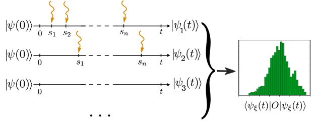
Figure 1: Scheme of the dynamical protocol. We consider a system prepared in a fixed initial state $\ket{\psi(0)}=\ket{a_{0}}$, undergoing random projective measurements of an observable $A$ (see Eq. (1)). Measurements occur with a fixed rate $\gamma$ at times $s_{1}<s_{2}<...$, whereas in the intervals $(s_{j},s_{j+1})$ the system follows an unitary time evolution. Different quantum trajectories are labelled by the integer $\xi$. The ensemble of states $\ket{\psi_{\xi}(t)}$ defines the probability distribution function of $\expectationvalue{O}{\psi_{\xi}(t)}$ (right).

$$p(x,t|s_{n},a_{n};\dots;s_{1},a_{1};0,a_{0})=\mathscr{D}(x,a_{n},t-s_{n})p(s_{n},a_{n}|s_{n-1},a_{n-1})\dots p(s_{1},a_{1}|0,a_{0}),$$ (6)

where the delta contribution can be rewritten as

$$\mathscr{D}(x,a,t)=\delta\big{(}x-\sum_{a^{\prime}=1}^{N}o_{a^{\prime}}\,p(t,a^{\prime}|0,a)\big{)},$$ (7)

and gives the contribution to the probability due to the last time-interval $(s_{n},t)$. In addition, the transition probabilities between eigenstates of ${A}$ read

$$p(s^{\prime},a^{\prime}|s,a)\equiv\mathbb{T}_{a^{\prime},a}(s^{\prime}-s)=\absolutevalue{\matrixelement{a^{\prime}}{U(s^{\prime}-s)}{a}}^{2}.$$ (8)

Let us assume that the transition matrix $\mathbb{T}$ can be diagonalised, i.e. $\mathbb{T}(s^{\prime}-s)=\mathbb{V}\,\mathbb{D}(s^{\prime}-s)\,\mathbb{V}^{\dagger}$ with eigenvalues $\mathbb{D}_{\alpha,\beta}(t)=d_{\alpha}(t)\delta_{\alpha,\beta}$, and time-independent unitary matrix $\mathbb{V}$ whose columns are the orthonormal eigenvectors. Notice that, since $\mathbb{T}$ is a unitary-stochastic matrix, $d_{1}=1$ is the largest eigenvalue, meanwhile as a consequence of the Perron–Frobenius theorem $\absolutevalue{d_{\alpha}}\leq 1$ for $\alpha=2,\dots,N$, where the equality holds in case of degeneracy [57, 58]. In addition, since $\sum_{a}\mathbb{T}_{a,b}=\sum_{b}\mathbb{T}_{a,b}=1$, the eigenvector associated to largest eigenvalue is simply given by $\mathbb{V}_{a,1}=1/\sqrt{N}$. Now let us focus on the nontrivial $P^{(n>0)}_{O}(x;t)$. For each order $n$ and fixed states $\{a_{0},a_{n}\}$, the sum over all the the possible intermediate outcomes can be rewritten as

$$\sum_{a_{1},\dots,a_{n-1}}\mathbb{T}_{a_{n},a_{n-1}}(s_{n}-s_{n-1})\cdots\mathbb{T}_{a_{1},a_{0}}(s_{1})=\sum_{\alpha=1}^{N}\mathbb{V}_{a_{n},\alpha}\prod_{j=1}^{n}d_{\alpha}(s_{j}-s_{j-1})(\mathbb{V}^{{\dagger}})_{\alpha,a_{0}},$$ (9)

with starting time $s_{0}=0$. We thus get

$$P^{(n>0)}_{O}(x;t)=e^{-\gamma t}\sum_{n=1}^{\infty}\left[\int_{0}^{t}\gamma\differential s_{n}\sum_{a_{n}=1}^{N}\mathscr{D}(x,a_{n},t-s_{n})\sum_{\alpha=1}^{N}\mathbb{V}_{a_{n},\alpha}I_{n,\alpha}(s_{n})(\mathbb{V}^{{\dagger}})_{\alpha,a_{0}}\right]$$ (10)

where we defined the time-ordered integrals

$$I_{n,\alpha}(s_{n})=\int_{0}^{s_{n}}\gamma\differential s_{n-1}\,d_{\alpha}(s_{n}-s_{n-1})\,\dots\,\int_{0}^{s_{2}}\gamma\differential s_{1}\,d_{\alpha}(s_{2}-s_{1})d_{\alpha}(s_{1}),$$ (11)

which satisfy the following recursive relations

$$\begin{dcases}I_{1,\alpha}(s_{1})=d_{\alpha}(s_{1}),\\ I_{n,\alpha}(s_{n})=\int_{0}^{s_{n}}\gamma\differential s_{n-1}\,d_{\alpha}(s_{n}-s_{n-1})I_{n-1,\alpha}(s_{n-1}),\quad n>1.\end{dcases}$$ (12)

In Eq. (10) the sum over $n$ can be safely taken, since $s_{n}$ and $a_{n}$ are dummies variables. Thus, we can introduce $I_{\alpha}(s)=\sum_{n=1}^{\infty}I_{n,\alpha}(s)$ which satisfy the following linear Volterra integral equation of the second kind

$$I_{\alpha}(s)-d_{\alpha}(s)=\int_{0}^{s}\gamma\differential s^{\prime}\,d_{\alpha}(s-s^{\prime})I_{\alpha}(s^{\prime}).$$ (13)

Exploiting the Laplace transform of the integral kernel, i.e. $\mathscr{L}[d_{\alpha}](z)=\int_{0}^{\infty}e^{-zt}d_{\alpha}(t)\differential t$, we can easily solve the previous equation obtaining

$$I_{\alpha}(s)=\mathscr{L}^{-1}\left[\frac{\mathscr{L}[d_{\alpha}](z)}{1-\gamma\mathscr{L}[d_{\alpha}](z)}\right](s),$$ (14)

where $\mathscr{L}^{-1}[\dots]$ is the inverse Laplace transform. As expected, it easy to show that

$$\mathscr{L}[I_{\alpha}](z)=\frac{\mathscr{L}[d_{\alpha}](z)}{1-\gamma\mathscr{L}[d_{\alpha}](z)}=\sum_{n=1}^{\infty}\gamma^{n-1}\mathscr{L}[d_{\alpha}]^{n}(z)=\sum_{n=1}^{\infty}\mathscr{L}[I_{n,\alpha}](z),$$ (15)

thus identifying $\mathscr{L}[I_{n,\alpha}](z)=\gamma^{n-1}\mathscr{L}[d_{\alpha}]^{n}(z)$. We can finally collect all those results, further simplify and finding the following general expression for the probability distribution

$$P^{(n>0)}_{O}(x;t)=e^{-\gamma t}\sum_{a=1}^{N}\sum_{\alpha=1}^{N}\int_{0}^{t}\gamma\differential s\,\mathscr{D}(x,a,t-s)\mathbb{V}_{a,\alpha}I_{\alpha}(s)(\mathbb{V}^{{\dagger}})_{\alpha,a_{0}}.$$ (16)

Let us finally mention that using this expression we can easily compute the $k$-th moment of the distribution, defined as $\left\langle x^{k}\right\rangle_{P_{O}}=\int\differential x\,x^{k}P_{O}(x;t)=\overline{\expectationvalue{O}{\psi_{\xi}(t)}^{k}}$. The first moment ($k=1$) is particularly simple, since it does reduce to the expectation value of $O$ over the averaged density matrix $\overline{\ket{\psi_{\xi}(t)}\bra{\psi_{\xi}(t)}}$ whose dynamics is fully described by the Lindblad equation (see C). In particular, using that $\sum_{b}\mathbb{T}_{a,b}(t-s)\mathbb{V}_{b,\alpha}=d_{\alpha}(t-s)\mathbb{V}_{a,\alpha}$, we easily get

$$\left\langle x\right\rangle_{P_{O}}=e^{-\gamma t}\sum_{a=1}^{N}o_{a}\,\mathbb{T}_{a,a_{0}}(t)+e^{-\gamma t}\sum_{a=1}^{N}o_{a}\sum_{\alpha=1}^{N}\mathbb{V}_{a,\alpha}\left[\int_{0}^{t}\gamma\differential s\,d_{\alpha}(t-s)I_{\alpha}(s)\right](\mathbb{V}^{{\dagger}})_{\alpha,a_{0}},$$ (17)

which can be further simplified exploiting Eq. (13), finally obtaining

$$\left\langle x\right\rangle_{P_{O}}=e^{-\gamma t}\sum_{a=1}^{N}o_{a}\sum_{\alpha=1}^{N}\mathbb{V}_{a,\alpha}I_{\alpha}(t)(\mathbb{V}^{{\dagger}})_{\alpha,a_{0}}.$$ (18)

Let us stress that the simplified expression in Eq. (18) applies only for averages of diagonal observables. Every time we are interested in higher moments or probability distribution of non-diagonal operators, the computation have to be carried out from scratch, basically starting from Eq. (16). Finally, due to the properties of the transfer matrix $\mathbb{T}$, the stationary limit $t\to\infty$ of the previous average can be easily taken; in fact, only $\alpha=1$, with $I_{1}(t)=e^{\gamma t}$, will contribute to the sum over $\alpha$, leading to $\left\langle x\right\rangle_{P_{O}}\to\frac{1}{N}\sum_{a=1}^{N}o_{a}$, where we used the fact that $\mathbb{V}_{a,1}=1/\sqrt{N}$. As expected from the Lindblad dynamics, it does correspond to the expectation value of the operator $O$ over the infinite temperature state $\frac{1}{N}\sum_{a=1}^{N}\ket{a}\bra{a}$.

3 Two-level system

We start by considering a continuously monitored two-level system. Despite their simplicity, two-level systems are the fundamental building block of the most studied quantum many-body systems and therefore understanding their behavior is crucial. The system consists of a single spin-$1/2$, whose unitary evolution is governed by the following hamiltonian

$${H}=-J\sigma^{x},$$ (19)

where $\sigma^{\alpha}$ are the Pauli matrices with $\alpha=x,y,z$ and $\commutator{\sigma^{\alpha}}{\sigma^{\beta}}=2i\epsilon_{\alpha\beta\gamma}\sigma^{\gamma}$. The system is continuously monitored along $z$ with a rate $\gamma$ (therefore ${A}=\sigma^{z}$). We will denote with $\ket{\sigma}=\ket{+1},\ket{-1}$ the eigenstates of $\sigma^{z}$ with eigenvalue $\sigma=\pm 1$ respectively. We consider a two-level spin which starts from $\ket{+1}$ and we want to evaluate

$$P_{\sigma^{z}}(x;t)=\overline{\delta\left(\expectationvalue{\sigma^{z}}{\psi_{\xi}(t)}-x\right)}=P^{(n>0)}_{\sigma^{z}}(x;t)+P^{(0)}_{\sigma^{z}}(x;t)\,,$$ (20)

i.e. the probability distribution of the expectation value of ${O}=\sigma^{z}$. It is easy to find that $\mathbb{T}(t)=\cos(Jt)^{2}\mathbb{I}+\sin(Jt)^{2}\sigma^{x}$, and $\mathbb{V}=(\sigma^{z}+\sigma^{x})/\sqrt{2}$ whose columns are the eigenvectors of $\sigma^{x}$. As expected $d_{1}=1$ and $d_{2}(t)=\cos(\Omega t)$, where $\Omega=2J$ is the splitting between the energy eigenvalues of the system. Notice that, from these eigenvalues we can derive two recursion relations as in the integral equations (12), then, since $d_{1}=1$ we immediately get $I_{1}(s)=e^{\gamma s}$. In the following, we will simplify the notation $I_{2}(s)=I(s)$. Finally, we notice that $\mathscr{D}(x,\sigma_{n},t-s_{n})=\delta\big{(}x-\sigma_{n}\cos(\Omega(t-s_{n}))\big{)}$, from which we can compute the no-click contribution

$$P^{(0)}_{\sigma^{z}}(x;t)=e^{-\gamma t}\,\delta\big{(}x-\cos(\Omega t)\big{)}.$$ (21)

In order to find the full probability distribution, we can use equation (16) to write

$$P^{(n>0)}_{\sigma^{z}}(x;t)=\frac{e^{-\gamma t}}{2}\int_{0}^{t}\gamma\differential s\sum_{\sigma=\pm 1}\delta(x-{\sigma}\cos(\Omega(t-s)))\left[e^{\gamma s}+\sigma I(s)\right]$$ (22)

For a better understanding of the solution, we do not apply the Laplace method to solve the integral equation (13) for $I(s)$. Instead, we differentiate it twice with respect to $s$, which yields the following differential equation for $I(s)$

$$\ddot{I}=\gamma\dot{I}-\Omega^{2}I\\$$ (23)

with the initial conditions $I(0)=1$ and $\dot{I}(0)=\gamma$. This is the equation of motion of an “anti-damped” harmonic oscillator (since $\gamma>0$). The solution can be found easily using standard methods [59], obtaining

$$I(s)=e^{\gamma s/2}\left[\cosh(\frac{\Gamma s}{2})+\frac{\gamma}{\Gamma}\sinh(\frac{\Gamma s}{2})\right],$$ (24)

where we defined the following characteristic frequency $\Gamma=\sqrt{\gamma^{2}-4\Omega^{2}}$. As expected, we find three different regimes depending on the sign of $\gamma^{2}-4\Omega^{2}$. Let us analyze the behavior of the function $e^{-\gamma s/2}I(s)$. When $\gamma<2\Omega$, we have that $\Gamma$ is an imaginary quantity. Therefore, we find a regime in which the function oscillates with a frequency of $\Omega\sqrt{1-\gamma^{2}/(4\Omega^{2})}$, which is lower than the natural frequency $\Omega$. When $\gamma=2\Omega$, we get the critical regime for which the function $e^{-\gamma s/2}I(s)$ becomes linear, $\left(1+\gamma s/2\right)$. Finally, if $\gamma>2\Omega$, it grows exponentially with a rate $\gamma/2\sqrt{1-4\Omega^{2}/\gamma^{2}}$ smaller than $\gamma/2$.

Let us finally consider the Dirac-delta function contribution. Solving for $x-\sigma\cos(\Omega(t-s))=0$, we easily get

$$\tilde{s}_{k}=t\pm\frac{1}{\Omega}\arccos(x\sigma)+\frac{2\pi k}{\Omega},\quad k\in\mathbb{Z}.$$ (25)

Using the properties of the Dirac-delta distribution, we can rewrite it as

$$\delta(x-\sigma\cos(\Omega(t-s)))=\sum_{k\in\mathbb{Z}}\frac{\delta(s-\tilde{s}_{k})}{\Omega\sqrt{1-x^{2}}}.$$ (26)

Since in Eq. (22), the integral is taken over a finite interval $[0,t]$, we need to constraint the solutions $\tilde{s}_{k}$ in Eq. (25) only to those falling in that region. However, we may relax that condition by explicitly introducing the Heaviside step function $\theta(x)$, such that Eq. (22) finally reads

$$P^{(n>0)}_{\sigma^{z}}(x;t)=\frac{\gamma e^{-\gamma t}}{2\Omega\sqrt{1-x^{2}}}\sum_{\sigma=\pm 1}\sum_{k\in\mathbb{Z}}\left[e^{\gamma\tilde{s}_{k}}+\sigma I(\tilde{s}_{k})\right]\theta(t-\tilde{s}_{k})\theta(\tilde{s}_{k})\,,$$ (27)

where $\tilde{s}_{k}$ implicitly depends on $x$ and $t$ as well. In Figure 2, we plot the entire distribution $P_{\sigma^{z}}(x;t)$. As expected, at early time the probability is highly asymmetric, having support only in the vicinity of $x=1$. The no-click term is in fact localised at $x=\cos(\Omega t)$ but its weight is exponentially suppressed in time. The click contribution is also showing a nontrivial asymmetric evolution. Its behavior strongly depends on $\gamma$ indeed: in the oscillatory regime ($\gamma<2\Omega$), the probability distribution function bounces back and forth between the two extremes $x=\pm 1$ of its domain; after many oscillations, the number depending on the value of $\gamma$, it is expected to relax toward a symmetric distribution, the typical relaxation time being $\tau=2/\gamma$. For $\gamma>2\Omega$ the probability is not oscillating anymore and the relaxation time becomes $\tau=2/(\gamma-\Gamma)$. Interestingly, as the measurement rate is getting higher, the time needs for the magnetisation statistics to reach the equilibrium becomes larger and larger, diverging as $\tau\sim\gamma/\Omega^{2}$.

The first moment of $P_{\sigma^{z}}(x;t)$, namely the magnetisation average $\left\langle x\right\rangle_{P_{{\sigma^{z}}}}=e^{-\gamma t}I(t)$, does coincide with the expectation value over the averaged state (see B). Nevertheless, our approach allows to easily compute the fluctuations of the magnetization along the trajectories. Indeed, by means of Eqs. (21) and (22), we can easily get the second moment of the distribution

$$\left\langle x^{2}\right\rangle_{P_{{\sigma^{z}}}}=e^{-\gamma t}\int_{0}^{t}\gamma\differential s\cos(\Omega(t-s))^{2}e^{\gamma s}+e^{-\gamma t}\cos(\Omega t)^{2},$$ (28)

which simplifies to

$$\left\langle x^{2}\right\rangle_{P_{{\sigma^{z}}}}=\frac{\gamma^{2}+2\Omega^{2}}{\gamma^{2}+4\Omega^{2}}+\frac{e^{-\gamma t}}{2(\gamma^{2}+4\Omega^{2})}\left[2\gamma\Omega\sin(2\Omega t)+\Omega^{2}\cos(2\Omega t)\right],$$ (29)

and which cannot be computed using the a Lindblad approach since it corresponds to $\overline{\langle\psi_{\xi}(t)|\sigma_{z}|\psi_{\xi}(t)\rangle^{2}}$. In Figure 3, we represents $\left\langle x\right\rangle_{P_{{\sigma^{z}}}},\left\langle x^{2}\right\rangle_{P_{{\sigma^{z}}}}$ as a function of time for different values of the measurement rate $\gamma$.

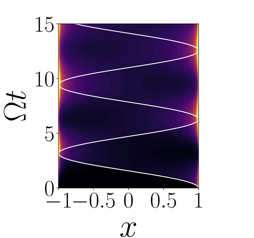
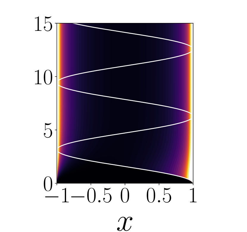
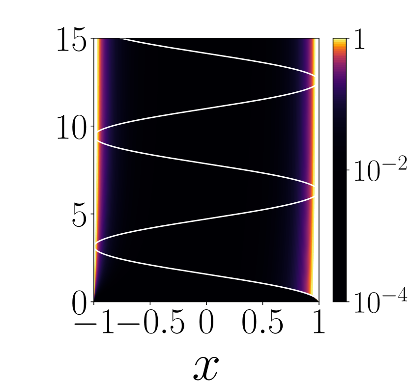
Figure 2: The time-dependent probability distribution $P_{\sigma^{z}}(x;t)$ for a two-level system ($\Omega=1$). The white continuous line represents the no-click contribution $P^{(0)}(x;t)$ in Eq. (21). We set $\gamma=0.2$ (left), $\gamma=2.0$ (center) and $\gamma=5.0$ (right).

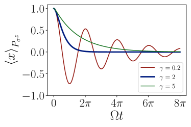
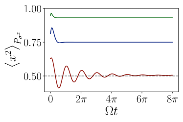
Figure 3: First (left) and second (right) moment of the probability distribution $P_{\sigma^{z}}(x;t)$ for a two-level system ($\Omega=1$). Notice that the critical value of $\gamma=2$ leads to the fastest convergence to the equilibrium stationary value of the average magnetization.

Finally, let us mention that one can easily obtain the asymptotic stationary distribution $P_{\sigma^{z}}(x,t\to\infty)$. Indeed, from a careful inspection of Eq. (22) one can argue that for large time the contribution coming from $I(s)$ is bounded by $e^{-\gamma t}\int_{0}^{t}\differential s|I(s)|$, thus decaying exponentially for large time. The only term that survives and contributes to the asymptotic stationary distribution is the one depending on $e^{\gamma s}$. Therefore, for any finite $\gamma$, the stationary distribution can be exactly evaluated as

$$P_{\sigma^{z}}(x)=\frac{\gamma}{2}\sum_{\sigma=\pm 1}\int_{0}^{\infty}\differential s\,\delta(x-\sigma\cos(\Omega s))e^{-\gamma s}=\frac{\gamma\left[e^{2\,\gamma\arcsin(x)/\Omega}+1\right]e^{\gamma\arccos(x)/\Omega}}{2\Omega\left(e^{\pi\gamma/\Omega}-1\right)\sqrt{1-x^{2}}},$$

which, as expected, is an even function of $x$. Interestingly, all (non-vanishing) stationary moments can be easily computed from the integral representation of the probability, namely

$$\left\langle x^{2n}\right\rangle_{P_{{\sigma^{z}}}}=\int_{0}^{\infty}ds\,e^{-s}\cos^{2n}(s\Omega/\gamma)=\frac{{}_{2}F_{1}(-2n,-n-i\gamma/(2\Omega);1-n-i\gamma/(2\Omega);-1)}{2^{2n}(1-2in\Omega/\gamma)},$$ (30)

while the odd moments are identically vanishing. In particular, when $\gamma\to\infty$, $\left\langle x^{2n}\right\rangle_{P_{{\sigma^{z}}}}\to 1$ for all $n$, confirming the fact that the stationary distribution converges to $[\delta(x-1)+\delta(x+1)]/2$.

4 Hopping particle

A free hopping quantum particle propagates in a lattice with a ballistic spreading. However, there are ways to prevent or slow down the propagation as, for instance, adding a disorder potential which induces Anderson localization [60, 61]. Here, we show that the quantum Zeno effect due to the coupling of the hopping particle to a measurement apparatus can also results into a slowdown of the particle propagation [62, 63]. Related protocols have been studied in the context of quantum stochastic resetting, in which the hopping particle is reset to the initial state with a certain probability [64].

We consider a simple hopping fermion on a 1D lattice, whose hamiltonian reads

$$H=-\Omega\sum_{j=1}^{L}\bigg{(}c^{\dagger}_{j}c_{j+1}+c^{\dagger}_{j+1}c_{j}\bigg{)}$$ (31)

with periodic boundary conditions (i.e. $c_{j+L}=c_{j}$). Here the lattice dimension $L$ (even) plays the role of an infrared cutoff. In the following we will take the limit $L\to\infty$ whenever it will be unambiguous. The Fermionic operator satisfy the canonical anti-commutation relations $\{c_{i},c^{{\dagger}}_{j}\}=\delta_{ij}$. We define the Fourier modes operators

$$\tilde{c}_{k}=\frac{1}{\sqrt{L}}\sum_{j}e^{ikj}c_{j},\quad c_{j}=\frac{1}{\sqrt{L}}\sum_{k}e^{-ikj}\tilde{c}_{k},$$ (32)

such that $\{\tilde{c}_{p},\tilde{c}^{{\dagger}}_{q}\}=\delta_{pq}$, and $k\in\{-\pi,-\pi+2\pi/L,-\pi+4\pi/L,\dots,\pi\}$. The Hamiltonian become diagonal in the Fourier representation, i.e. $H=\sum_{k}\varepsilon(k)\tilde{c}^{\dagger}_{k}\tilde{c}_{k}$, where $\varepsilon(k)=-2\Omega\cos k$. We now restrict the problem to the single-particle sector of the hamiltonian, we can define the states $\ket{j}=c^{\dagger}_{j}\ket{\emptyset}$ and $\ket*{\tilde{k}}=\tilde{c}^{\dagger}_{k}\ket{\emptyset}$, which represents the particle in position $j$ or with momentum $k$ respectively. Notice that $\innerproduct*{j}{\tilde{k}}=\exp(-ikj)/\sqrt{L}$ is the normalised wave function. Since $H$ commute with he total number of particles, the unitary dynamics can be restricted in such sector and it is governed by the following single-particle Hamiltonian

$$H=-\Omega\sum_{j=1}^{L}\left(\outerproduct{j}{j+1}+\outerproduct{j+1}{j}\right)=\sum_{k}\varepsilon(k)\outerproduct*{\tilde{k}}{\tilde{k}}.$$ (33)

We consider the particle initial localised at the origin $j=0$ of our lattice, namely $\ket{\psi_{\xi}(0)}=\ket{0}$ for all trajectories $\xi$. We then suppose to continuously measure, with a rate $\gamma$, the position operator

$$q=\sum_{j}j\outerproduct*{j}{j}.$$ (34)

We are thus interested in the displacement of the particle along each single trajectory, however, for symmetry reasons, when no measurement occurs (i.e. $\gamma=0$) the probability function of the outcome of $\langle q\rangle_{t}$ is time independent, namely $\overline{\delta\left(x-\langle q\rangle_{t}\right)}=\delta(0)$. This is not in contradiction with the expected ballistic spreading under the free evolution, which can be extracted when observing even power of $q$ (see C). Notice that, this is not true anymore when $\gamma\neq 0$. We are thus interested in the probability distribution function of the particle displacement itself, namely

$$P_{q}(x;t)=\overline{\delta\left(\expectationvalue{q}{\psi_{\xi}(t)}-x\right)}=P^{(n>0)}_{q}(x;t)+P^{(0)}_{q}(x;t),$$ (35)

where in this case the no-click contribution is trivially given by $P^{(0)}_{q}(x;t)=e^{-\gamma t}\delta(x)$, and we used the following results for the evolution amplitudes in the thermodynamic limit

$$\matrixelement{j}{U(t)}{l}=\sum_{k}\matrixelement*{j}{e^{-itH}}{\tilde{k}}\innerproduct*{\tilde{k}}{l} =\int_{-\pi}^{\pi}\frac{\differential k}{2\pi}e^{i\left[k(j-l)-2t\Omega\cos k\right]} =(-i)^{j-l}J_{j-l}(2\Omega t),$$ (36)

with $J_{n}(x)$ being the Bessel function of the first kind. Now the transition probability matrix reads $\mathbb{T}_{i,j}(t)=J^{2}_{i-j}(2\Omega t)$, which is a circulant matrix due to translational invariance. Let us define the not normalised eigenvectors whose component are $\mathbb{V}_{n,k}=e^{-ink}$, such that

$$(\mathbb{T}(t)\mathbb{V})_{n,k}=\sum_{j}J^{2}_{n-j}(2\Omega t)e^{-ijk}=e^{-ink}\sum_{l}J^{2}_{j}(2\Omega t)e^{ilk}\equiv\mathbb{V}_{n,k}\,d_{k}(t)$$ (37)

where we identified the eigenvalues of the transfer matrix as $d_{k}(t)=\sum_{l}J^{2}_{l}(2\Omega t)e^{ikl}=J_{0}[\omega_{k}t]$, with $\omega_{k}=4\Omega\sin(k/2)$. Following Section 2, we can easily solve the integral equation (13) for $I_{k}(s)=\sum_{n=1}^{\infty}I_{n,k}(s)$ with kernel $J_{0}[\omega_{k}t]$; the Laplace transform reads

$$\mathscr{L}[I_{k}](z)=\frac{1}{\sqrt{z^{2}+\omega_{k}^{2}}-\gamma}=\sum_{n=1}^{\infty}\frac{\gamma^{n-1}}{(z^{2}+\omega_{k}^{2})^{n/2}},$$ (38)

and we can identify with $\mathscr{L}[I_{n,k}](z)$ the terms of the series expansion, thus finally getting

$$I_{n,k}(s)=\sqrt{\pi}\gamma^{n-1}\left(\frac{s}{2|\omega_{k}|}\right)^{\frac{n-1}{2}}\frac{J_{\frac{n-1}{2}}(s|\omega_{k}|)}{\Gamma\left(n/2\right)}.$$ (39)

With a simple generalization of equation (10), we can write the click contribution to the probability distribution as

$$P^{(n>0)}_{q}(x;t)=e^{-\gamma t}\sum_{j}\int_{0}^{t}\gamma\differential s\int_{-\pi}^{\pi}\frac{\differential k}{2\pi}\mathscr{D}(x,j,t-s)e^{-ijk}I_{k}(s),$$ (40)

where, thanks to the properties of the Bessel functions, the delta contribution reduces to $\mathscr{D}(x,j,t-s)=\delta(x-j)$, which basically says that the probability has only support on $x\in\mathbb{Z}$. The entire probability distribution $P_{q}(x;t)$ is represented in Figure 4 together with some representative quantum trajectories for different values of $\gamma$.

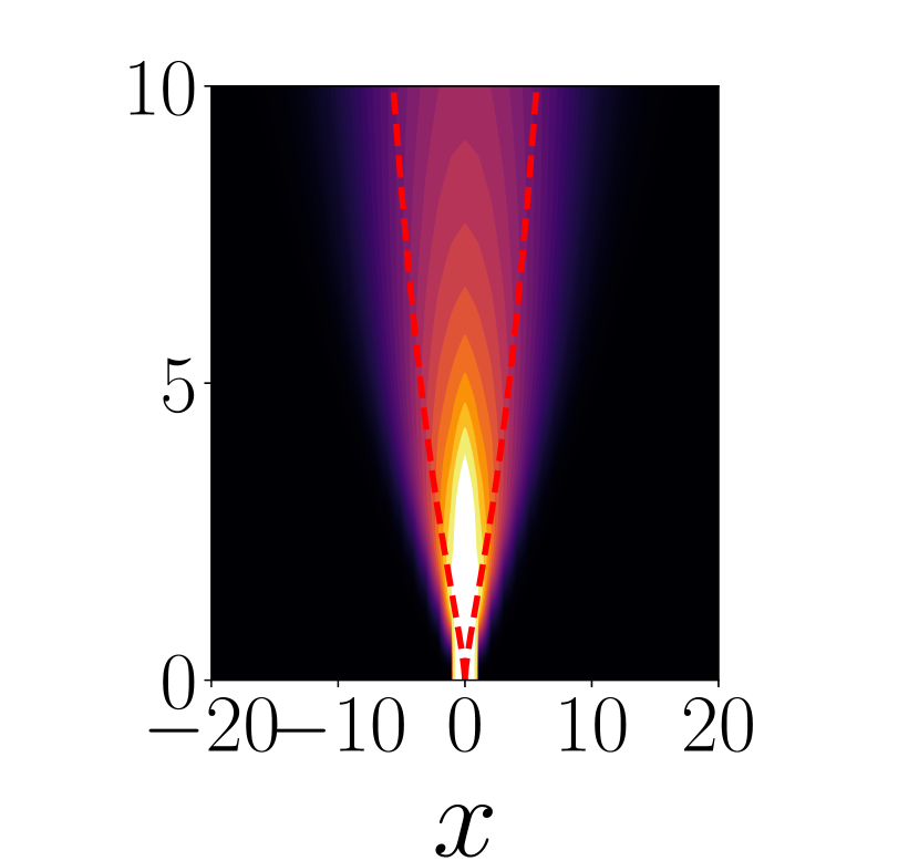
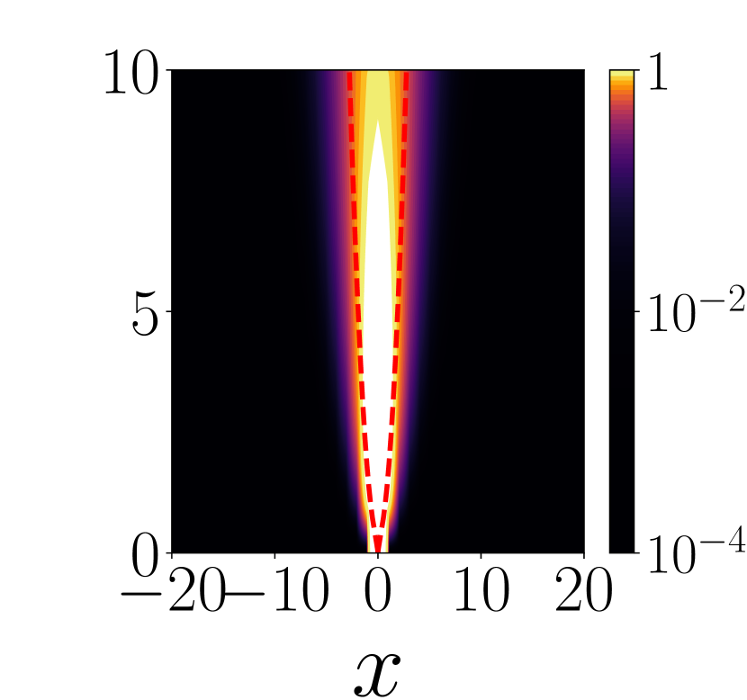
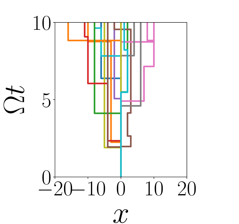
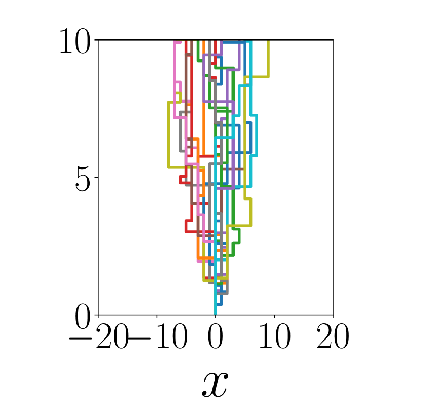
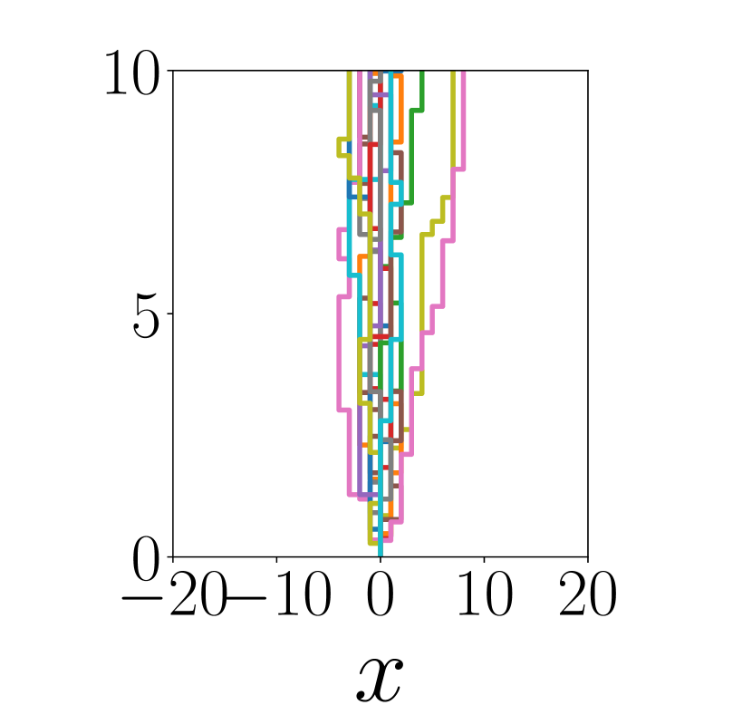
Figure 4: Upper panels: the time-dependent probability distribution $P_{q}(x;t)$ for an hopping particle ($\Omega=1$). Red lines represents the standard deviation $\pm\left\langle x^{2}\right\rangle_{P_{q}}^{1/2}$ as in Eq. (42). We set $\gamma=0.25$ (left), $\gamma=1.0$ (center) and $\gamma=5.0$ (right). Lower panels: the expectation value $\expectationvalue{q}{\psi_{\xi}(t)}$ for $20$ trajectories and the same values of $\gamma$.

We have previously observed that the first moment of the probability distribution is identically vanishing due to the inversion symmetry. The second moment instead gets a nontrivial contribution from the $P^{(n>0)}_{q}$ part, thus reading

$$\left\langle x^{2}\right\rangle_{P_{q}}=e^{-\gamma t}\int_{0}^{t}\gamma\differential s\,\int_{-\pi}^{\pi}\frac{\differential k}{2\pi}\left[\sum_{j}j^{2}e^{-ijk}\right]I_{k}(s),$$ (41)

which can be further simplified using the identity $\sum_{j}j^{2}e^{-ijk}=-\sum_{j}\partial_{k}^{2}e^{ijk}=-2\pi\delta^{\prime\prime}(k),$ leading to

$$\left\langle x^{2}\right\rangle_{P_{q}}=-e^{-\gamma t}\int_{0}^{t}\gamma\differential s\,[\partial^{2}_{k}I_{k}(s)]\bigr{\rvert}_{k=0}=\frac{4\Omega^{2}}{\gamma^{2}}\left[(\gamma t-2)+e^{-\gamma t}(\gamma t+2)\right].$$ (42)

The second moment does behave differently depending on the time-scale, showing the following scaling behaviour

$$\left\langle x^{2}\right\rangle_{P_{q}}\sim\begin{dcases}\gamma\Omega^{2}t^{3}\quad\gamma t\ll 1\\ \frac{4\Omega^{2}t}{\gamma}\quad\gamma t\gg 1\end{dcases}.$$ (43)

Let us mention that the fluctuations of the $P_{q}(x;t)$ distribution cannot give information about the ballistic behavior at $\gamma=0$, due to the inversion symmetry. As a matter of fact, what Eq. (43) gives us is the leading term for $\gamma\neq 0$. In the asymptotic regime $\gamma t\gg 1$, it does coincide (as expected) with $\left\langle x\right\rangle_{P_{q^{2}}}$ confirming the diffusive behavior for any finite measurement rate. However, in the $\gamma t\ll 1$ regime, the $O(\gamma^{0})$ term is missing, and it is recovered in the expansion of $\left\langle x\right\rangle_{P_{q^{2}}}$ (see C).

5 Conclusions

In this article, we have presented an approach for studying the dynamics of quantum systems undergoing unitary evolution and continuous monitoring. Our approach goes beyond the traditional Lindblad master equation and provides a more complete picture of the system’s behavior by considering the entire ensemble of stochastic quantum trajectories.

Specifically, we have developed an analytical tool to compute the probability distribution of the expectation value of a given observable over the ensemble of quantum trajectories. We obtained exact formulas to evaluate this probability distribution and its moments for two paradigmatic examples: a single qubit subjected to magnetization measurements, and a free hopping particle subjected to position measurements.

Our results demonstrate that the probability distribution of expectation values can exhibit non-trivial features that are missed by traditional approaches, highlighting the full properties contained in the set of quantum trajectories in the analysis of continuously monitored quantum systems.

Note added.—While completing this work, the preprint [65] appeared, dealing with topics related to the ones discussed by us.

Acknowledgments

This work was supported by the PNRR MUR project PE0000023-NQSTI

Appendix A Useful properties of the Bessel Functions

Here we collect some properties of the Bessel functions

$$J_{n}(t)=\frac{1}{2\pi}\int_{-\pi}^{\pi}\differential z\,e^{i\left(nz-t\sin z\right)},$$ (44)

which have been used all along the main text. Let’s start by noticing that $J_{n}(t)^{2}$ are non-negative and normalized over $\mathbb{Z}$, i.e. $\sum_{n\in\mathbb{Z}}J_{n}(t)^{2}=1$. In other words, they can be interpreted as probabilities over the infinite set of discrete events $n\in\mathbb{Z}$, with a parameter dependence $t$. They indeed satisfy the following property

$$\sum_{n\in\mathbb{Z}}x^{2n}J_{n}(t)^{2}=J_{0}[it(x-1/x)],$$ (45)

from which we can easily define the generating function $F_{t}(\lambda)$ of the moments of the distribution, as

$$F_{t}(\lambda)\equiv\sum_{n\in\mathbb{Z}}e^{i\lambda n}J_{n}^{2}(t)=J_{0}[2t\sin(\lambda/2)],$$ (46)

such that $\sum_{n\in\mathbb{Z}}n^{k}J_{n}(t)^{2}=(-i)^{k}\partial^{k}_{\lambda}F_{t}(\lambda)$. From the previous relation it is straightforward to show that

$$\int_{-\pi}^{\pi}\frac{\differential\lambda}{2\pi}e^{-i\lambda n}J_{0}[2t\sin(\lambda/2)]=J^{2}_{n}(t)$$ (47)

Finally, another useful property of the Bessel functions is that it is possible to compute the Laplace Transform, which reads

$$\mathscr{L}[J_{n}](z)=\frac{\left(z+\sqrt{z^{2}+1}\right)^{-n}}{\sqrt{z^{2}+1}}.$$ (48)

Appendix B Lindblad equation solution for the two level system

When we are interested in the dynamical map averaged over the quantum trajectories, the measurement protocol outlined in the main text can be reformulated in terms of a Lindblad equation for the averaged density matrix $\rho(t)=\overline{\outerproduct{\psi_{\xi}(t)}{\psi_{\xi}(t)}}$. In fact, averaging over different trajectories does correspond to relax both the information on whether the spin has been measured, and the result of the measurement itself. See [66] for some results of projective measurement-based dissipation descriptions of Lindblad equations for quantum spin systems.

In particular for a single spin undergoing projective measurements of $\sigma^{z}$ (see Sec. 3), the average state $\rho$ transforms accordingly to

$$\rho(t)\to\left(1-\frac{\gamma dt}{2}\right)\rho(t)+\frac{\gamma dt}{2}\sigma^{z}\,\rho(t)\,\sigma^{z},$$ (49)

where $\gamma dt$ is the probability that the system is measured, after a discretization of the continuum time evolution has been applied.

Combining the previous expansion with the unitary part of the evolution, and taking the continuum limit $dt\to 0$ with $\gamma$ fixed, we finally get the following Lindblad master equation

$$\partial_{t}\rho=-i[H,\rho]+\frac{\gamma}{2}\left(\sigma^{z}\,\rho\,\sigma^{z}-\rho\right),$$ (50)

with $H=-J\sigma^{x}$. This equation can be easily solved by expanding the density operator in the basis of Pauli matrices

$$\rho(t)=\frac{1}{2}\mathbb{I}+\frac{1}{2}\sum_{\alpha=1}^{3}m_{\alpha}(t)\sigma^{\alpha},$$ (51)

where $m_{\alpha}(t)=\Tr[\sigma^{\alpha}\rho(t)]$ and $\mathbb{I}$ is the $2\times 2$ identity matrix. The Lindblad equation becomes a linear differential equation for the three components of the magnetisation $(m_{x},m_{y},m_{z})^{T}$, which reads

$$\partial_{t}\begin{pmatrix}m_{x}\\ m_{y}\\ m_{z}\end{pmatrix}=\begin{pmatrix}-\gamma&0&0\\ 0&-\gamma&\Omega\\ 0&-\Omega&0\end{pmatrix}\begin{pmatrix}m_{x}\\ m_{y}\\ m_{z}\end{pmatrix}$$ (52)

where $\Omega=2J$. The $z$ component evolves following the differential equation of a damped harmonic oscillator $\partial^{2}_{t}m_{z}=-\Omega^{2}m_{z}-\gamma\partial_{t}m_{z}$, with initial condition $m_{z}(0)=1$, $\partial_{t}m_{z}(0)=0$. From the solution of such equation we easily recover the result of the main text, namely

$$m_{z}(t)=e^{-\gamma t/2}\left[\cosh(\frac{\Gamma t}{2})+\frac{\gamma}{\Gamma}\sinh(\frac{\Gamma t}{2})\right]\equiv\left\langle x\right\rangle_{P_{\sigma^{z}}}$$ (53)

with $\Gamma=\sqrt{\gamma^{2}-4\Omega^{2}}$. In addition, we also gets

$$m_{x}(t)=0,\quad m_{y}(t)=e^{-\gamma t/2}\frac{2\Omega}{\Gamma}\sinh(\frac{\Gamma t}{2}).$$ (54)

Appendix C Lindblad equation solution for the hopping particle

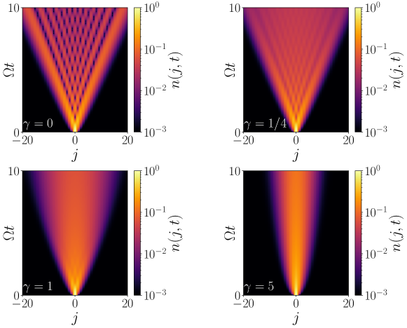
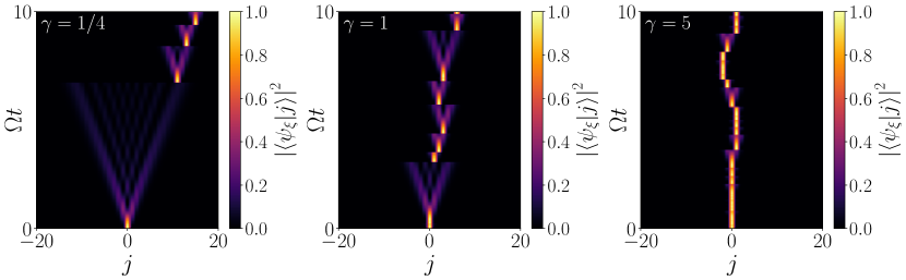
Figure 5: Upper four panels: average local particle density $n(j,t)$ obtained from the average state given by Lindblad equation (Eq. 56). Different measurement rates are considered (i.e. $\gamma=0,0.25,1,5$), showing a clear transition from a ballistic to a diffusive dynamics. Lower three panels: the local particle density $|\langle\psi_{\xi}|j\rangle|^{2}$ obtained from quantum trajectories at different measurement rates ($\gamma=0.25,1,5$).

In the case of the hopping particle, to analyze the dynamical map averaged over quantum trajectories, we can again reframe the measurement procedure as a Lindblad equation for the averaged density matrix $\rho(t)$. When we perform projective measurements of the particle’s position at a rate $\gamma$, the average state $\rho$ undergoes the following transformation in accordance with the usual rules of quantum mechanics

$$\rho(t)\to\left(1-\gamma\differential t\right)\rho(t)+\gamma\differential t\sum_{j}\pi_{j}\rho(t)\pi_{j}\,.$$ (55)

Here, $\pi_{j}=\outerproduct{j}{j}$ represents the projectors over the lattice sites. The Lindblad master equation can be obtained by taking the limit $\differential t\to 0$ with a fixed value of $\gamma$, resulting in

$$\partial_{t}\rho=-i\commutator{H}{\rho}+\gamma\left[\sum_{j}\pi_{j}\rho\pi_{j}-\rho\right],$$ (56)

with $H$ as in Eq. 33. In the case of a system with finite size, we can solve numerically the dynamical map

$$\rho(t+\differential t)=\rho(t)-i\differential t\left(H\rho-\rho H\right)+\gamma\differential t\left[\sum_{j}\pi_{j}\rho(t)\pi_{j}-\rho(t)\right],$$ (57)

and define the site densities $n(j,t)=\Tr{\rho(t)\pi_{j}}$ as depicted in the upper four panels in Fig. 5. In accordance to what have been discussed in the main text, the averages over the probability distribution coincides with the expectation values taken over the averaged state.

Now, we collect few results for the first moment of some relevant observables. In particular, from the probability distribution of a generic power $q^{m}$, by using the generic equation (18) we explicitly get

$$\left\langle x\right\rangle_{P_{q^{m}}}=\Tr{\rho(t)q^{m}}=e^{-\gamma t}\int_{-\pi}^{\pi}\frac{\differential k}{2\pi}\sum_{j}j^{m}e^{-ijk}I_{k}(t)\,.$$ (58)

By exploiting $\sum_{j}j^{m}e^{-ijk}=i^{m}2\pi\delta^{(m)}(k)$, we obtain

$$\left\langle x\right\rangle_{P_{q^{m}}}=i^{m}e^{-\gamma t}\partial^{m}_{k}I_{k}(t)|_{k=0}.$$ (59)

As expected, $\left\langle x\right\rangle_{P_{q}}=0$, while the first non-vanishing average occurs for $m=2$, giving

$$\left\langle x\right\rangle_{P_{q^{2}}}=\frac{4\Omega^{2}\left(\gamma t+e^{-\gamma t}-1\right)}{\gamma^{2}}\sim\begin{dcases}2\Omega^{2}t^{2}\quad\gamma t\ll 1\\ \frac{4\Omega^{2}t}{\gamma}\quad\gamma t\gg 1\end{dcases}$$ (60)

thus, we recover the ballistic behavior at early time (or for $\gamma=0$), whilst a diffusive behavior for any $\gamma\neq 0$ at large time, with a diffusion constant $D_{\gamma}=2\Omega^{2}/\gamma$ such that $\left\langle x_{q_{2}}\right\rangle\sim 2D_{\gamma}t$. This behavior has been observed in the many-body description of the model, in particular studying the particle current after quenching an initial domain wall configuration [24]. Due to its linear nature, this exact result can be compared with the solution of the Lindblad equation. Indeed, the average of $q^{2}$ is also given by $\left\langle x\right\rangle_{P_{q^{2}}}=\sum_{j}j^{2}n(j,t)$, where $n(j,t)=\Tr{\rho(t)\pi_{j}}$ can be evaluated numerically (see Fig. 5 upper panels), or analytically taking the average over the probability distribution associated to $\pi_{j}$

$$P_{\pi_{j}}(x;t)=\overline{\delta\left(\expectationvalue{\pi_{j}}{\psi_{\xi}(t)}-x\right)}.$$ (61)

Explicitly we get

$$\left\langle x\right\rangle_{P_{\pi_{j}}}=n(j,t)=e^{-\gamma t}\int_{-\pi}^{\pi}\frac{\differential k}{2\pi}e^{-ijk}I_{k}(t),$$ (62)

notice that, as expected, $\sum_{j}n(j,t)=1$, since $I_{0}(t)=e^{\gamma t}$.

References

- [1] R. Penrose “The Road to Reality: A Complete Guide to the Laws of the Universe”, Science: Astrophysics Jonathan Cape, 2004 URL: https://books.google.it/books?id=csaaQgAACAAJ
- [2] John Neumann and Robert T. Beyer “Mathematical Foundations of Quantum Mechanics: New Edition” Princeton University Press, 2018 DOI: 10.23943/princeton/9780691178561.001.0001
- [3] John Archibald Wheeler and Wojciech Hubert Zurek “Quantum theory and measurement” Princeton University Press, 2014
- [4] Alexander S Holevo “Statistical structure of quantum theory” Springer Berlin, Heidelberg, 2003 DOI: https://doi.org/10.1007/3-540-44998-1
- [5] Angelo Bassi et al. “Models of wave-function collapse, underlying theories, and experimental tests” In Rev. Mod. Phys. 85 American Physical Society, 2013, pp. 471–527 DOI: 10.1103/RevModPhys.85.471
- [6] Howard M. Wiseman and Gerard J. Milburn “Quantum Measurement and Control” Cambridge University Press, 2009 DOI: 10.1017/CBO9780511813948
- [7] Niels Henrik David Bohr “The Quantum Postulate and the Recent Development of Atomic Theory” In Nature 121, 1928, pp. 580–590 DOI: https://doi.org/10.1038/121580a0
- [8] N. Katz et al. “Coherent State Evolution in a Superconducting Qubit from Partial-Collapse Measurement” In Science 312.5779, 2006, pp. 1498–1500 DOI: 10.1126/science.1126475
- [9] P. Campagne-Ibarcq et al. “Observing Quantum State Diffusion by Heterodyne Detection of Fluorescence” In Phys. Rev. X 6 American Physical Society, 2016, pp. 011002 DOI: 10.1103/PhysRevX.6.011002
- [10] Philipp M. Preiss et al. “Strongly correlated quantum walks in optical lattices” In Science 347.6227, 2015, pp. 1229–1233 DOI: 10.1126/science.1260364
- [11] Adam Smith, MS Kim, Frank Pollmann and Johannes Knolle “Simulating quantum many-body dynamics on a current digital quantum computer” In npj Quantum Information 5.1 Nature Publishing Group UK London, 2019, pp. 106 DOI: https://doi.org/10.1038/s41534-019-0217-0
- [12] Alessandro Santini and Vittorio Vitale “Experimental violations of Leggett-Garg inequalities on a quantum computer” In Phys. Rev. A 105 American Physical Society, 2022, pp. 032610 DOI: 10.1103/PhysRevA.105.032610
- [13] John Preskill “Quantum Computing in the NISQ era and beyond” In Quantum 2 Verein zur Förderung des Open Access Publizierens in den Quantenwissenschaften, 2018, pp. 79 DOI: 10.22331/q-2018-08-06-79
- [14] Luis Pedro Garcı́a-Pintos, Diego Tielas and Adolfo Campo “Spontaneous Symmetry Breaking Induced by Quantum Monitoring” In Phys. Rev. Lett. 123 American Physical Society, 2019, pp. 090403 DOI: 10.1103/PhysRevLett.123.090403
- [15] Michele Campisi, Peter Talkner and Peter Hänggi “Fluctuation Theorems for Continuously Monitored Quantum Fluxes” In Phys. Rev. Lett. 105 American Physical Society, 2010, pp. 140601 DOI: 10.1103/PhysRevLett.105.140601
- [16] Andrea Solfanelli, Lorenzo Buffoni, Alessandro Cuccoli and Michele Campisi “Maximal energy extraction via quantum measurement” In Journal of Statistical Mechanics: Theory and Experiment 2019.9 IOP PublishingSISSA, 2019, pp. 094003 DOI: 10.1088/1742-5468/ab3721
- [17] Lorenzo Buffoni et al. “Quantum Measurement Cooling” In Phys. Rev. Lett. 122 American Physical Society, 2019, pp. 070603 DOI: 10.1103/PhysRevLett.122.070603
- [18] Guido Giachetti, Stefano Gherardini, Andrea Trombettoni and Stefano Ruffo “Quantum-Heat Fluctuation Relations in Three-Level Systems Under Projective Measurements” In Condensed Matter 5.1, 2020 DOI: 10.3390/condmat5010017
- [19] S. Gherardini, G. Giachetti, S. Ruffo and A. Trombettoni “Thermalization processes induced by quantum monitoring in multilevel systems” In Phys. Rev. E 104 American Physical Society, 2021, pp. 034114 DOI: 10.1103/PhysRevE.104.034114
- [20] Andrea Solfanelli, Alessandro Santini and Michele Campisi “Experimental Verification of Fluctuation Relations with a Quantum Computer” In PRX Quantum 2 American Physical Society, 2021, pp. 030353 DOI: 10.1103/PRXQuantum.2.030353
- [21] Stefano Gherardini et al. “Energy fluctuation relations and repeated quantum measurements” In Chaos, Solitons & Fractals 156, 2022, pp. 111890 DOI: https://doi.org/10.1016/j.chaos.2022.111890
- [22] Gonzalo Manzano and Roberta Zambrini “Quantum thermodynamics under continuous monitoring: A general framework” 025302 In AVS Quantum Science 4.2, 2022 DOI: 10.1116/5.0079886
- [23] Alessandro Santini, Andrea Solfanelli, Stefano Gherardini and Guido Giachetti “Observation of partial and infinite-temperature thermalization induced by continuous monitoring on a quantum hardware” In arXiv, 2022 DOI: 10.48550/ARXIV.2211.07444
- [24] Xiangyu Cao, Antoine Tilloy and Andrea De Luca “Entanglement in a fermion chain under continuous monitoring” In SciPost Phys. 7 SciPost, 2019, pp. 024 DOI: 10.21468/SciPostPhys.7.2.024
- [25] M Buchhold, Y Minoguchi, A Altland and S Diehl “Effective theory for the measurement-induced phase transition of Dirac fermions” In Physical Review X 11.4 APS, 2021, pp. 041004 DOI: https://doi.org/10.1103/PhysRevX.11.041004
- [26] Thomas Müller, Sebastian Diehl and Michael Buchhold “Measurement-induced dark state phase transitions in long-ranged fermion systems” In Physical Review Letters 128.1 APS, 2022, pp. 010605 DOI: https://doi.org/10.1103/PhysRevLett.128.010605
- [27] Alberto Biella and Marco Schiró “Many-body quantum Zeno effect and measurement-induced subradiance transition” In Quantum 5 Verein zur Förderung des Open Access Publizierens in den Quantenwissenschaften, 2021, pp. 528 DOI: https://doi.org/10.22331/q-2021-08-19-528
- [28] Piotr Sierant et al. “Dissipative Floquet Dynamics: from Steady State to Measurement Induced Criticality in Trapped-ion Chains” In Quantum 6 Verein zur Förderung des Open Access Publizierens in den Quantenwissenschaften, 2022, pp. 638 DOI: 10.22331/q-2022-02-02-638
- [29] Xhek Turkeshi, Marcello Dalmonte, Rosario Fazio and Marco Schirò “Entanglement transitions from stochastic resetting of non-Hermitian quasiparticles” In Physical Review B 105.24 APS, 2022, pp. L241114
- [30] Shraddha Sharma, Xhek Turkeshi, Rosario Fazio and Marcello Dalmonte “Measurement-induced criticality in extended and long-range unitary circuits” In SciPost Physics Core 5.2, 2022, pp. 023
- [31] Piotr Sierant and Xhek Turkeshi “Universal behavior beyond multifractality of wave functions at measurement-induced phase transitions” In Physical Review Letters 128.13 APS, 2022, pp. 130605 DOI: https://doi.org/10.1103/PhysRevLett.128.130605
- [32] Michele Coppola, Emanuele Tirrito, Dragi Karevski and Mario Collura “Growth of entanglement entropy under local projective measurements” In Physical Review B 105.9 APS, 2022, pp. 094303 DOI: https://doi.org/10.1103/PhysRevB.105.094303
- [33] Giulia Piccitto, Angelo Russomanno and Davide Rossini “Entanglement transitions in the quantum Ising chain: A comparison between different unravelings of the same Lindbladian” In Physical Review B 105.6 APS, 2022, pp. 064305
- [34] Xhek Turkeshi, Lorenzo Piroli and Marco Schiró “Enhanced entanglement negativity in boundary-driven monitored fermionic chains” In Phys. Rev. B 106 American Physical Society, 2022, pp. 024304 DOI: 10.1103/PhysRevB.106.024304
- [35] Marcin Szyniszewski, Alessandro Romito and Henning Schomerus “Entanglement transition from variable-strength weak measurements” In Physical Review B 100.6 APS, 2019, pp. 064204 DOI: https://doi.org/10.1103/PhysRevB.100.064204
- [36] T. Boorman, M. Szyniszewski, H. Schomerus and A. Romito “Diagnostics of entanglement dynamics in noisy and disordered spin chains via the measurement-induced steady-state entanglement transition” In Phys. Rev. B 105 American Physical Society, 2022, pp. 144202 DOI: 10.1103/PhysRevB.105.144202
- [37] Emanuele Tirrito, Alessandro Santini, Rosario Fazio and Mario Collura “Full counting statistics as probe of measurement-induced transitions in the quantum Ising chain” In arXiv, 2023 DOI: https://doi.org/10.48550/arXiv.2212.09405
- [38] Giulia Piccitto, Angelo Russomanno and Davide Rossini “Entanglement dynamics with string measurement operators” In arXiv, 2023 DOI: https://doi.org/10.48550/arXiv.2303.07102
- [39] Graham Kells, Dganit Meidan and Alessandro Romito “Topological transitions in weakly monitored free fermions” In SciPost Phys. 14 SciPost, 2023, pp. 031 DOI: 10.21468/SciPostPhys.14.3.031
- [40] Alessio Paviglianiti and Alessandro Silva “Multipartite Entanglement in the Measurement-Induced Phase Transition of the Quantum Ising Chain” In arXiv, 2023 DOI: https://doi.org/10.48550/arXiv.2302.06477
- [41] Caterina Zerba and Alessandro Silva “Measurement phase transitions in the no-click limit as quantum phase transitions of a non-hermitean vacuum” In arXiv, 2023 DOI: https://doi.org/10.48550/arXiv.2301.07383
- [42] Yuri Minoguchi, Peter Rabl and Michael Buchhold “Continuous gaussian measurements of the free boson CFT: A model for exactly solvable and detectable measurement-induced dynamics” In SciPost Physics 12.1 Stichting SciPost, 2022 DOI: 10.21468/scipostphys.12.1.009
- [43] Marcin Szyniszewski, Alessandro Romito and Henning Schomerus “Universality of entanglement transitions from stroboscopic to continuous measurements” In Physical review letters 125.21 APS, 2020, pp. 210602 DOI: https://doi.org/10.1103/PhysRevLett.125.210602
- [44] Xhek Turkeshi, Rosario Fazio and Marcello Dalmonte “Measurement-induced criticality in (2+ 1)-dimensional hybrid quantum circuits” In Physical Review B 102.1 APS, 2020, pp. 014315 DOI: https://doi.org/10.1103/PhysRevB.102.014315
- [45] Chao-Ming Jian, Yi-Zhuang You, Romain Vasseur and Andreas W.. Ludwig “Measurement-induced criticality in random quantum circuits” In Phys. Rev. B 101 American Physical Society, 2020, pp. 104302 DOI: 10.1103/PhysRevB.101.104302
- [46] Ori Alberton, Michael Buchhold and Sebastian Diehl “Entanglement Transition in a Monitored Free-Fermion Chain: From Extended Criticality to Area Law” In Physical Review Letters 126.17 APS, 2021, pp. 170602 DOI: https://doi.org/10.1103/PhysRevLett.126.170602
- [47] Xhek Turkeshi et al. “Measurement-induced entanglement transitions in the quantum Ising chain: From infinite to zero clicks” In Physical Review B 103.22 APS, 2021, pp. 224210 DOI: https://doi.org/10.1103/PhysRevB.103.224210
- [48] Xhek Turkeshi “Measurement-induced criticality as a data-structure transition” In Physical Review B 106.14 APS, 2022, pp. 144313 DOI: https://doi.org/10.1103/PhysRevB.106.144313
- [49] Thomas Botzung, Sebastian Diehl and Markus Müller “Engineered dissipation induced entanglement transition in quantum spin chains: from logarithmic growth to area law” In Physical Review B 104.18 APS, 2021, pp. 184422 DOI: https://doi.org/10.1103/PhysRevB.104.184422
- [50] Matthias M. Müller, Stefano Gherardini and Filippo Caruso “Quantum Zeno Dynamics Through Stochastic Protocols” In Annalen der Physik 529.9, 2017, pp. 1600206 DOI: https://doi.org/10.1002/andp.201600206
- [51] Parveen Kumar, Alessandro Romito and Kyrylo Snizhko “Quantum Zeno effect with partial measurement and noisy dynamics” In Phys. Rev. Res. 2 American Physical Society, 2020, pp. 043420 DOI: 10.1103/PhysRevResearch.2.043420
- [52] Matteo Ippoliti and Vedika Khemani “Postselection-free entanglement dynamics via spacetime duality” In Physical Review Letters 126.6 APS, 2021, pp. 060501 DOI: https://doi.org/10.1103/PhysRevLett.126.060501
- [53] Jin Ming Koh, Shi-Ning Sun, Mario Motta and Austin J. Minnich “Experimental Realization of a Measurement-Induced Entanglement Phase Transition on a Superconducting Quantum Processor” In arXiv, 2022 DOI: https://doi.org/10.48550/arXiv.2203.04338
- [54] Howard M Wiseman “Quantum trajectories and quantum measurement theory” In Quantum and Semiclassical Optics: Journal of the European Optical Society Part B 8.1 IOP Publishing, 1996, pp. 205 DOI: 10.1088/1355-5111/8/1/015
- [55] Martin B Plenio and Peter L Knight “The quantum-jump approach to dissipative dynamics in quantum optics” In Reviews of Modern Physics 70.1 APS, 1998, pp. 101 DOI: https://doi.org/10.1103/RevModPhys.70.101
- [56] Heinz-Peter Breuer and Francesco Petruccione “The theory of open quantum systems” Oxford University Press on Demand, 2002
- [57] Karol Zyczkowski, Marek Kus, Wojciech Słomczyński and Hans-Jürgen Sommers “Random unistochastic matrices” In Journal of Physics A: Mathematical and General 36.12, 2003, pp. 3425 DOI: 10.1088/0305-4470/36/12/333
- [58] Crispin Gardiner “Stochastic methods” Springer Berlin, Heidelberg, 2009 URL: https://link.springer.com/book/9783540707127
- [59] David Morin “Introduction to Classical Mechanics: With Problems and Solutions” Cambridge University Press, 2008 DOI: 10.1017/CBO9780511808951
- [60] P.. Anderson “Absence of Diffusion in Certain Random Lattices” In Phys. Rev. 109 American Physical Society, 1958, pp. 1492–1505 DOI: 10.1103/PhysRev.109.1492
- [61] Antonello Scardicchio and Thimothée Thiery “Perturbation theory approaches to Anderson and Many-Body Localization: some lecture notes”, 2017 arXiv:1710.01234 [cond-mat.dis-nn]
- [62] Kiran E. Khosla, Ardalan Armin and M.. Kim “Quantum trajectories, interference, and state localisation in dephasing assisted quantum transport”, 2021 DOI: https://doi.org/10.48550/arXiv.2111.02986
- [63] Debraj Das and Shamik Gupta “Quantum random walk and tight-binding model subject to projective measurements at random times” In Journal of Statistical Mechanics: Theory and Experiment 2022.3 IOP PublishingSISSA, 2022, pp. 033212 DOI: 10.1088/1742-5468/ac5dc0
- [64] B. Mukherjee, K. Sengupta and Satya N. Majumdar “Quantum dynamics with stochastic reset” In Phys. Rev. B 98 American Physical Society, 2018, pp. 104309 DOI: 10.1103/PhysRevB.98.104309
- [65] Christian Carisch, Alessandro Romito and Oded Zilberberg “Quantifying measurement-induced quantum-to-classical crossover using an open-system entanglement measure” In arXiv, 2023 DOI: https://doi.org/10.48550/arXiv.2304.02965
- [66] Zi Cai and Thomas Barthel “Algebraic versus Exponential Decoherence in Dissipative Many-Particle Systems” In Phys. Rev. Lett. 111 American Physical Society, 2013, pp. 150403 DOI: 10.1103/PhysRevLett.111.150403