Neural Exploitation and Exploration of Contextual Bandits

Abstract

In this paper, we study utilizing neural networks for the exploitation and exploration of contextual multi-armed bandits. Contextual multi-armed bandits have been studied for decades with various applications. To solve the exploitation-exploration trade-off in bandits, there are three main techniques: epsilon-greedy, Thompson Sampling (TS), and Upper Confidence Bound (UCB). In recent literature, a series of neural bandit algorithms have been proposed to adapt to the non-linear reward function, combined with TS or UCB strategies for exploration. In this paper, instead of calculating a large-deviation based statistical bound for exploration like previous methods, we propose, “EE-Net,” a novel neural-based exploitation and exploration strategy. In addition to using a neural network (Exploitation network) to learn the reward function, EE-Net uses another neural network (Exploration network) to adaptively learn the potential gains compared to the currently estimated reward for exploration. We provide an instance-based $\widetilde{\mathcal{O}}(\sqrt{T})$ regret upper bound for EE-Net and show that EE-Net outperforms related linear and neural contextual bandit baselines on real-world datasets.

Keywords: Multi-armed Bandits, Neural Contextual Bandits, Neural Networks, Exploitation and Exploration, Regret Analysis

1 Introduction

The stochastic contextual multi-armed bandit (MAB) (Lattimore and Szepesvári, 2020) has been studied for decades in the machine learning community to solve sequential decision making, with applications in online advertising (Li et al., 2010), personalized recommendation (Wu et al., 2016; Ban and He, 2021b), etc. In the standard contextual bandit setting, a set of $n$ arms are presented to a learner in each round, where each arm is represented by a context vector. Then by a certain strategy, the learner selects and plays one arm, receiving a reward. The goal of this problem is to maximize the cumulative rewards of $T$ rounds.

MAB problems have principled approaches to address the trade-off between Exploitation and Exploration (EE), as the collected data from past rounds should be exploited to get good rewards and under-explored arms need to be explored with the hope of getting even better rewards. The most widely used approaches for EE trade-off can be classified into three main techniques: Epsilon-greedy (Langford and Zhang, 2008), Thompson Sampling (TS) (Thompson, 1933; Kveton et al., 2021), and Upper Confidence Bound (UCB) (Auer, 2002; Ban and He, 2020).

Linear bandits (Li et al., 2010; Dani et al., 2008; Abbasi-Yadkori et al., 2011), where the reward is assumed to be a linear function with respect to arm vectors, have been well studied and succeeded both empirically and theoretically. Given an arm, ridge regression is usually adapted to estimate its reward based on collected data from past rounds. UCB-based algorithms (Li et al., 2010; Chu et al., 2011; Wu et al., 2016; Ban and He, 2021b) calculate an upper bound for the confidence ellipsoid of estimated reward, and determine the arm according to the sum of estimated reward and UCB. TS-based algorithms (Agrawal and Goyal, 2013; Abeille and Lazaric, 2017) formulate each arm as a posterior distribution where the mean is the estimated reward, and choose the one with the maximal sampled reward. However, the linear assumption regarding the reward may not be true in real-world applications (Valko et al., 2013).

To learn non-linear reward functions, recent works have utilized deep neural networks to learn the underlying reward functions, thanks to the powerful representation ability. Considering the past selected arms and received rewards as training samples, a neural network $f_{1}$ is built for exploitation. Zhou et al. (2020) computes a gradient-based upper confidence bound with respect to $f_{1}$ and uses the UCB strategy to select arms. Zhang et al. (2021) formulates each arm as a normal distribution where the mean is $f_{1}$ and the standard deviation is calculated based on the gradient of $f_{1}$, and then uses the TS strategy to choose arms. Both Zhou et al. (2020) and Zhang et al. (2021) achieve the near-optimal regret bound of $O(\sqrt{T}\log T)$.

Figure 1 (2) provide the main motivation for this work by carefully investigating the exploration mechanism. Based on the difference between the estimated reward and the expected reward, the exploration may be divided into two types: "upward" exploration and "downward" exploration. The upward exploration formulates the cases where the expected reward is larger than the estimated reward. In other words, the learner’s model underestimated the reward, and thus it is required to add another value to the estimated reward to minimize the gap between expected and estimated rewards. The downward exploration describes the cases where the expected reward is smaller than the estimated reward. This indicates that the model overestimated the reward. Hence, we intend to subtract a value from the estimated reward to narrow the gap between the expected and estimated reward. Here, we inspect the three main exploration strategies in these two types of exploration. First, the UCB-based approaches always add a positive value to the estimated reward. This is enabled to do the upward exploration, while avoiding the downward exploration. Second, the TS-based methods draw a sampled reward from some formulated distribution where the mean is the estimated reward. Due to that the formulated distribution usually is symmetric, e.g., normal distribution, it will randomly make upward and downward exploration. Third, for the epsilon-greedy algorithms, with probability epsilon, it will make pure random exploration, but this exploration is completely stochastic and not based on the estimated reward.

Figure 1: Left figure: Structure of EE-Net. In the right figure, Case 1: "Upward" exploration should be made when the learner underestimates the reward; Case 2: "Downward" exploration should be chosen when the learner overestimates the reward. EE-Net has the ability to adaptively make exploration according to different cases. In contrast, UCB-based strategy will always make upward exploration, and TS-based strategy will randomly choose upward or downward exploration.

In this paper, we propose a novel neural exploitation and exploration strategy named "EE-Net." Similar to other neural bandits, EE-Net has an exploitation network $f_{1}$ to estimate the reward for each arm. The crucial difference from existing works is that EE-Net has an exploration network $f_{2}$ to predict the potential gain for each arm compared to the current reward estimate. The input of the exploration network $f_{2}$ is the gradient of $f_{1}$ to incorporate the information of arms and the discriminative ability of $f_{1}$. The ground truth for training $f_{2}$ is the residual between the received reward and the estimated reward by $f_{1}$, to equip with the ability to predict the exploration direction. Finally, we combine the two neural networks together, $f_{1}$ and $f_{2}$, to select the arms. Figure 1 depicts the workflow of EE-Net and its advantages for exploration compared to UCB or TS-based methods (see more details in Appendix A.2). To sum up, the contributions of this paper can be summarized as follows:

1. We propose a novel neural exploitation-exploration strategy in contextual bandits, EE-Net, where another neural network is assigned to learn the potential gain compared to the current reward estimate for adaptive exploration.

2. Under mild assumptions of over-parameterized neural networks, we provide an instance-based $\widetilde{\mathcal{O}}(\sqrt{T})$ regret upper bound of for EE-Net, where the complexity term in this bound is easier to interpret, and this bound improves by a multiplicative factor of $\sqrt{\log T}$ and is independent of either the input or the effective dimension, compared to related bandit algorithms.

3. We conduct experiments on four real-world datasets, showing that EE-Net outperforms baselines, including linear and neural versions of $\epsilon$-greedy, TS, and UCB.

Next, we discuss the problem definition in Sec.3, elaborate on the proposed EE-Net in Sec.4, and present our theoretical analysis in Sec.5. In the end, we provide the empirical evaluation (Sec.6) and conclusion (Sec.7).

2 Related Work

Constrained Contextual bandits. The common constraint placed on the reward function is the linear assumption, usually calculated by ridge regression (Li et al., 2010; Abbasi-Yadkori et al., 2011; Valko et al., 2013; Dani et al., 2008). The linear UCB-based bandit algorithms (Abbasi-Yadkori et al., 2011; Li et al., 2016) and the linear Thompson Sampling (Agrawal and Goyal, 2013; Abeille and Lazaric, 2017) can achieve satisfactory performance and the near-optimal regret bound of $\tilde{\mathcal{O}}(\sqrt{T})$. To relax the linear assumption, (Filippi et al., 2010) generalizes the reward function to a composition of linear and non-linear functions and then adopts a UCB-based algorithm to estimate it; (Bubeck et al., 2011) imposes the Lipschitz property on the reward metric space and constructs a hierarchical optimization approach to make selections; (Valko et al., 2013) embeds the reward function into Reproducing Kernel Hilbert Space and proposes the kernelized TS/UCB bandit algorithms.

Neural Bandits. To learn non-linear reward functions, deep neural networks have been adapted to bandits with various variants. Riquelme et al. (2018); Lu and Van Roy (2017) build $L$-layer DNNs to learn the arm embeddings and apply Thompson Sampling on the last layer for exploration. Zhou et al. (2020) first introduces a provable neural-based contextual bandit algorithm with a UCB exploration strategy and then Zhang et al. (2021) extends the neural network to TS framework. Their regret analysis is built on recent advances on the convergence theory in over-parameterized neural networks (Du et al., 2019; Allen-Zhu et al., 2019) and utilizes Neural Tangent Kernel (Jacot et al., 2018; Arora et al., 2019) to construct connections with linear contextual bandits (Abbasi-Yadkori et al., 2011). Ban and He (2021a) further adopts convolutional neural networks with UCB exploration aiming for visual-aware applications. Xu et al. (2020) performs UCB-based exploration on the last layer of neural networks to reduce the computational cost brought by gradient-based UCB. Qi et al. (2022) study utilizing the correlation among arms in contextual bandits. Different from the above existing works, EE-Net keeps the powerful representation ability of neural networks to learn the reward function and, for the first time, uses another neural network for exploration.

3 Problem definition

We consider the standard contextual multi-armed bandit with the known number of rounds $T$ (Zhou et al., 2020; Zhang et al., 2021). In each round $t\in[T]$, where the sequence $[T]=[1,2,\dots,T]$, the learner is presented with $n$ arms, $\mathbf{X}_{t}=\{\mathbf{x}_{t,1},\dots,\mathbf{x}_{t,n}\}$, in which each arm is represented by a context vector $\mathbf{x}_{t,i}\in\mathbb{R}^{d}$ for each $i\in[n]$. After playing one arm $\mathbf{x}_{t,i}$, its reward $r_{t,i}$ is assumed to be generated by the function:

$$r_{t,i}=h(\mathbf{x}_{t,i})+\eta_{t,i},$$ (3.1)

where the unknown reward function $h(\mathbf{x}_{t,i})$ can be either linear or non-linear and the noise $\eta_{t,i}$ is drawn from a certain distribution with expectation $\mathbb{E}[\eta_{t,i}]=0$. Note that we do not impose any assumption on the distribution of $\eta_{t,i}$. Following many existing works (Zhou et al., 2020; Ban et al., 2021; Zhang et al., 2021), we consider bounded rewards, $r_{t,i}\in[0,1],t\in[T],i\in[n]$. Let $\mathbf{x}_{t,\widehat{i}}$ be the selected arm and $r_{t,\widehat{i}}$ be the received reward in round $t$. The pseudo regret of $T$ rounds is defined as:

$$\mathbf{R}_{T}=\mathbb{E}\left[\sum_{t=1}^{T}(r_{t,i^{\ast}}-r_{t,\widehat{i}})\right],$$ (3.2)

where $i^{\ast}=\arg\max_{i\in[n]}h(\mathbf{x}_{t,i})$ is the index of the arm with the maximal expected reward in round $t$. The goal of this problem is to minimize $\mathbf{R}_{T}$ by a certain selection strategy.

Notation. We denote by $\{\mathbf{x}_{i}\}_{i=1}^{t}$ the sequence $(\mathbf{x}_{1},\dots,\mathbf{x}_{t})$. We use $\|v\|_{2}$ to denote the Euclidean norm for a vector $v$, and $\|\mathbf{W}\|_{2}$ and $\|\mathbf{W}\|_{F}$ to denote the spectral and Frobenius norm for a matrix $\mathbf{W}$. We use $\langle\cdot,\cdot\rangle$ to denote the standard inner product between two vectors or two matrices. We may use $\triangledown_{\boldsymbol{\theta}^{1}_{t}}f_{1}(\mathbf{x}_{t,i})$ or $\triangledown_{\boldsymbol{\theta}^{1}_{t}}f_{1}$ to represent the gradient $\triangledown_{\boldsymbol{\theta}^{1}_{t}}f_{1}(\mathbf{x}_{t,i};\boldsymbol{\theta}^{1}_{t})$ for brevity. We use $\{\mathbf{x}_{\tau},r_{\tau}\}_{\tau=1}^{t}$ to represent the collected data up to round $t$.

4 Proposed Method: EE-Net

EE-Net is composed of two components. The first component is the exploitation network, $f_{1}(\cdot;\boldsymbol{\theta}^{1})$, which focuses on learning the unknown reward function $h$ based on the data collected in past rounds. The second component is the exploration network, $f_{2}(\cdot;\boldsymbol{\theta}^{2})$, which focuses on characterizing the level of exploration needed for each arm in the present round.

1) Exploitation Net. The exploitation net $f_{1}$ is a neural network which learns the mapping from arms to rewards. In round $t$, denote the network by $f_{1}(\cdot;\boldsymbol{\theta}^{1}_{t-1})$, where the superscript of $\boldsymbol{\theta}_{t-1}^{1}$ is the index of the network and the subscript represents the round where the parameters of $f_{1}$ finish the last update. Given an arm $\mathbf{x}_{t,i},i\in[n]$, $f_{1}(\mathbf{x}_{t,i};\boldsymbol{\theta}^{1}_{t-1})$ is considered the "exploitation score" for $\mathbf{x}_{t,i}$ by exploiting the past data. By some criterion, after playing arm $\mathbf{x}_{t,\widehat{i}}$, we receive a reward $r_{t,\widehat{i}}$. Therefore, we can conduct stochastic gradient descent (SGD) to update $\boldsymbol{\theta}^{1}_{t-1}$ based on $(\mathbf{x}_{t,\widehat{i}},r_{t,\widehat{i}})$ and denote the updated parameters by $\boldsymbol{\theta}^{1}_{t}$.

Algorithm 1 EE-Net

1:$f_{1},f_{2}$, $T$ (number of rounds), $\eta_{1}$ (learning rate for $f_{1}$), $\eta_{2}$ (learning rate for $f_{2}$), $\phi$ (normalization operator)

2:Initialize $\boldsymbol{\theta}^{1}_{0},\boldsymbol{\theta}^{2}_{0}$; $\mathcal{H}_{0}=\emptyset$

3:for  $t=1,2,\dots,T$ do

4:     Observe $n$ arms $\{\mathbf{x}_{t,1},\dots,\mathbf{x}_{t,n}\}$

5:     for each $i\in[n]$  do

6:         Compute $f_{1}(\mathbf{x}_{t,i};\boldsymbol{\theta}^{1}_{t-1}),f_{2}(\phi(\mathbf{x}_{t,i});\boldsymbol{\theta}^{2}_{t-1})$

7:     end for

8:     $\widehat{i}=\arg\max_{i\in[n]}\left(f_{1}(\mathbf{x}_{t,i};\boldsymbol{\theta}^{1}_{t-1})+f_{2}(\phi(\mathbf{x}_{t,i});\boldsymbol{\theta}^{2}_{t-1})\right)$    

9:     Play $\mathbf{x}_{t,\widehat{i}}$ and observe reward $r_{t,\widehat{i}}$

10:     $\mathcal{L}_{1}=\frac{1}{2}\left(f_{1}(\mathbf{x}_{t,\widehat{i}};\boldsymbol{\theta}^{1}_{t-1})-r_{t,\widehat{i}}\right)^{2}$

11:     $\boldsymbol{\theta}^{1}_{t}=\boldsymbol{\theta}^{1}_{t-1}-\eta_{1}\triangledown_{\boldsymbol{\theta}^{1}_{t-1}}\mathcal{L}_{1}$

12:     $\mathcal{L}_{2}=\frac{1}{2}\left(f_{2}(\phi(\mathbf{x}_{t,\widehat{i}}));\boldsymbol{\theta}^{2}_{t-1})-(r_{t,\widehat{i}}-f_{1}(\mathbf{x}_{t,\widehat{i}};\boldsymbol{\theta}^{1}_{t-1}))\right)^{2}$

13:     $\boldsymbol{\theta}^{2}_{t}=\boldsymbol{\theta}^{2}_{t-1}-\eta_{2}\triangledown_{\boldsymbol{\theta}^{2}_{t-1}}\mathcal{L}_{2}$

14:end for

2) Exploration Net. Our exploration strategy is inspired by existing UCB-based neural bandits (Zhou et al., 2020; Ban et al., 2021). Given an arm $\mathbf{x}_{t,i}$, with probability at least $1-\delta$, it has the following UCB form:

$$|h(\mathbf{x}_{t,i})-f_{1}(\mathbf{x}_{t,i};\boldsymbol{\theta}^{1}_{t-1})|\leq g(\nabla_{\boldsymbol{\theta}^{1}_{t-1}}f_{1}(\mathbf{x}_{t,i};\boldsymbol{\theta}^{1}_{t-1})),$$ (4.1)

where $h$ is defined in Eq. (3.1) and $g$ is an upper confidence bound represented by a function with respect to the gradient $\nabla_{\boldsymbol{\theta}^{1}_{t-1}}f_{1}$ (see more details and discussions in Appendix A.2). Then we have the following definition.

Definition 4.1 (Potential Gain).

In round $t$, given an arm $\mathbf{x}_{t,i}$, we define $h(\mathbf{x}_{t,i})-f_{1}(\mathbf{x}_{t,i};\boldsymbol{\theta}^{1}_{t-1})$ as the "expected potential gain" for $\mathbf{x}_{t,i}$ and $r_{t,i}-f_{1}(\mathbf{x}_{t,i};\boldsymbol{\theta}^{1}_{t-1})$ as the "potential gain" for $\mathbf{x}_{t,i}$.

Let $y_{t,i}=r_{t,i}-f_{1}(\mathbf{x}_{t,i};\boldsymbol{\theta}^{1}_{t-1})$. When $y_{t,i}>0$, the arm $\mathbf{x}_{t,i}$ has positive potential gain compared to the estimated reward $f_{1}(\mathbf{x}_{t,i};\boldsymbol{\theta}^{1}_{t-1})$. A large positive $y_{t,i}$ makes the arm more suitable for upward exploration while a large negative $y_{t,i}$ makes the arm more suitable for downward exploration. In contrast, $y_{t,i}$ with a small absolute value makes the arm unsuitable for exploration. Recall that traditional approaches such as UCB intend to estimate such potential gain $y_{t,i}$ using standard tools, e.g., Markov inequality, Hoeffding bounds, etc., from large deviation bounds.

Instead of calculating a large-deviation based statistical bound for $y_{t,i}$, we use a neural network $f_{2}(\cdot;\boldsymbol{\theta}^{2})$ to represent $g$, where the input is $\nabla_{\boldsymbol{\theta}^{1}_{t-1}}f_{1}(\mathbf{x}_{t,i})$ and the ground truth is $r_{t,i}-f_{1}(\mathbf{x}_{t,i};\boldsymbol{\theta}^{1}_{t-1})$. Adopting gradient $\nabla_{\boldsymbol{\theta}^{1}_{t-1}}f_{1}(\mathbf{x}_{t,i})$ as the input is due to the fact that it incorporates two aspects of information: the features of the arm and the discriminative information of $f_{1}$.

Moreover, in the upper bound of NeuralUCB (Zhou et al., 2020) or the variance of NeuralTS (Zhang et al., 2021), there is a recursive term $\mathbf{A}_{t-1}=\mathbf{I}+\sum_{\tau=1}^{t-1}\nabla_{\boldsymbol{\theta}^{1}_{\tau-1}}f_{1}(\mathbf{x}_{\tau,\widehat{i}})\nabla_{\boldsymbol{\theta}^{1}_{\tau-1}}f_{1}(\mathbf{x}_{\tau,\widehat{i}})^{\top}$ which is a function of past gradients up to $(t-1)$ and incorporates relevant historical information. On the contrary, in EE-Net, the recursive term which depends on past gradients is $\boldsymbol{\theta}^{2}_{t-1}$ in the exploration network $f_{2}$ because we have conducted gradient descent for $\boldsymbol{\theta}^{2}_{t-1}$ based on $\{\nabla_{\boldsymbol{\theta}^{1}_{\tau-1}}f_{1}(\mathbf{x}_{\tau,\widehat{i}})\}_{\tau=1}^{t-1}$. Therefore, this form $\boldsymbol{\theta}^{2}_{t-1}$ is similar to $\mathbf{A}_{t-1}$ in neuralUCB/TS, but EE-net does not (need to) make a specific assumption about the functional form of past gradients, and it is also more memory-efficient.

To sum up, in round $t$, we consider $f_{2}(\nabla_{\boldsymbol{\theta}^{1}_{t-1}}f_{1}(\mathbf{x}_{t,i});\boldsymbol{\theta}^{2}_{t-1})$ as the "exploration score" of $\mathbf{x}_{t,i}$ to make the adaptive exploration, because it indicates the potential gain of $\mathbf{x}_{t,i}$ compared to our current exploitation score $f_{1}(\mathbf{x}_{t,i};\boldsymbol{\theta}^{1}_{t-1})$. Therefore, after receiving the reward $r_{t}$, we can use gradient descent to update $\boldsymbol{\theta}^{2}$ based on collected training samples $\{\nabla_{\boldsymbol{\theta}^{1}_{\tau-1}}f_{1}(\mathbf{x}_{\tau,\widehat{i}}),r_{\tau}-f_{1}(\mathbf{x}_{\tau,\widehat{i}};\boldsymbol{\theta}^{1}_{\tau-1}\}_{\tau=1}^{t}$. We also provide another two heuristic forms for $f_{2}$’s ground-truth label: $|r_{t,i}-f_{1}(\mathbf{x}_{t,i};\boldsymbol{\theta}^{1}_{t-1})|$ and $\text{ReLU}(r_{t,i}-f_{1}(\mathbf{x}_{t,i};\boldsymbol{\theta}^{1}_{t-1}))$.

Remark 4.1 (Network structure).

The networks $f_{1},f_{2}$ can have different structures according to different applications. For example, in the vision tasks, $f_{1}$ can be set up as convolutional layers (LeCun et al., 1995). For the exploration network $f_{2}$, the input $\nabla_{\boldsymbol{\theta}^{1}}f_{1}$ may have exploding dimensions when the exploitation network $f_{1}$ becomes wide and deep, which may cause huge computation cost for $f_{2}$. To address this challenge, we can apply dimensionality reduction techniques to obtain low-dimensional vectors of $\nabla_{\boldsymbol{\theta}^{1}}f_{1}$. In the experiments, we use Roweis and Saul (2000) to acquire a $10$-dimensional vector for $\nabla_{\boldsymbol{\theta}^{1}}f_{1}$ and achieve the best performance among all baselines.∎

Remark 4.2 (Exploration direction).

EE-Net has the ability to determine the exploration direction. Given an arm $\mathbf{x}_{t,i}$, when the estimate $f_{1}(\mathbf{x}_{t,i})$ is lower than the expected reward $h(\mathbf{x}_{t,i})$, the learner should make the "upward" exploration, i.e., increase the chance of $\mathbf{x}_{t,i}$ being explored; when $f_{1}(\mathbf{x}_{t,i})$ is higher than $h(\mathbf{x}_{t,i})$, the learner should do the "downward" exploration, i.e., decrease the chance of $\mathbf{x}_{t,i}$ being explored. EE-Net uses the neural network $f_{2}$ to learn $h(\mathbf{x}_{t,i})-f_{1}(\mathbf{x}_{t,i})$ (which has positive or negative scores), and has the ability to determine the exploration direction. In contrast, NeuralUCB will always make "upward" exploration and NeuralTS will randomly choose between "upward" exploration and "downward" exploration (see selection criteria in Table 3 and more details in Appendix A.2). ∎

Remark 4.3 (Space complexity).

NeuralUCB and NeuralTS have to maintain the gradient outer product matrix (e.g., $\mathbf{A}_{t}=\sum_{\tau=1}^{t}\nabla_{\boldsymbol{\theta}^{1}}f_{1}(\mathbf{x}_{\tau,\widehat{i}};\boldsymbol{\theta}^{1}_{\tau})\nabla_{\boldsymbol{\theta}^{1}}f_{1}(\mathbf{x}_{\tau,\widehat{i}};\boldsymbol{\theta}^{1}_{\tau})^{\top}\in\mathbb{R}^{p_{1}\times p_{1}}$ and $\boldsymbol{\theta}^{1}\in\mathbb{R}^{p_{1}}$) has a space complexity of $O(p_{1}^{2})$ to store the outer product. On the contrary, EE-Net does not have this matrix and only regards $\nabla_{\boldsymbol{\theta}^{1}}f_{1}$ as the input of $f_{2}$. Thus, EE-Net reduces the space complexity from $\mathcal{O}(p^{2}_{1})$ to $\mathcal{O}(p_{1})$. ∎

Table 1: Structure of EE-Net (Round $t$).

Input	Network	Label
$\{\mathbf{x}_{\tau,\widehat{i}}\}_{\tau=1}^{t}$	$f_{1}(\cdot;\boldsymbol{\theta}^{1})$ (Exploitation)	$\{r_{\tau}\}_{\tau=1}^{t}$
$\{\nabla_{\boldsymbol{\theta}_{\tau-1}^{1}}f_{1}(\mathbf{x}_{\tau,\widehat{i}};\boldsymbol{\theta}_{\tau-1}^{1})\}_{\tau=1}^{t}$	$f_{2}(\cdot;\boldsymbol{\theta}^{2})$ (Exploration)	$\left\{\left(r_{\tau}-f_{1}(\mathbf{x}_{\tau,\widehat{i}};\boldsymbol{\theta}_{\tau-1}^{1})\right)\right\}_{\tau=1}^{t}$

5 Regret Analysis

In this section, we provide the regret analysis of EE-Net. Then, for the analysis, we have the following assumption, which is a standard input assumption in neural bandits and over-parameterized neural networks (Zhou et al., 2020; Allen-Zhu et al., 2019).

Assumption 5.1.

For any $t\in[T],i\in[n],\|\mathbf{x}_{t,i}\|_{2}=1$, and $r_{t,i}\in[0,1]$.

The analysis will focus on over-parameterized neural networks (Jacot et al., 2018; Du et al., 2019; Allen-Zhu et al., 2019). Given an input $\mathbf{x}\in\mathbb{R}^{d}$, without loss of generality, we define the fully-connected network $f$ with depth $L\geq 2$ and width $m$:

$$f(\mathbf{x};\boldsymbol{\theta})=\mathbf{W}_{L}\sigma(\mathbf{W}_{L-1}\sigma(\mathbf{W}_{L-2}\dots\sigma(\mathbf{W}_{1}\mathbf{x})))$$ (5.1)

where $\sigma$ is the ReLU activation function, $\mathbf{W}_{1}\in\mathbb{R}^{m\times d}$, $\mathbf{W}_{l}\in\mathbb{R}^{m\times m}$, for $2\leq l\leq L-1$, $\mathbf{W}^{L}\in\mathbb{R}^{1\times m}$, and $\boldsymbol{\theta}=[\text{vec}(\mathbf{W}_{1})^{\intercal},\text{vec}(\mathbf{W}_{2})^{\intercal},\dots,\text{vec}(\mathbf{W}_{L})^{\intercal}]^{\intercal}\in\mathbb{R}^{p}$ .

Initialization. For any $l\in[L-1]$, each entry of $\mathbf{W}_{l}$ is drawn from the normal distribution $\mathcal{N}(0,\frac{2}{m})$ and $\mathbf{W}_{L}$ is drawn from the normal distribution $\mathcal{N}(0,\frac{1}{m})$. $f_{1}$ and $f_{2}$ both follow above network structure but with different input and output, denoted by $f_{1}(\mathbf{x};\boldsymbol{\theta}^{1}),\boldsymbol{\theta}^{1}\in\mathbb{R}^{p_{1}},f_{2}(\phi(\mathbf{x});\boldsymbol{\theta}^{2}),\boldsymbol{\theta}^{2}\in\mathbb{R}^{p_{2}}$. Here, we use $\phi(\mathbf{x})$ to represent the input of $f_{2}$, which can be designed as $\phi(\mathbf{x}_{t,i})=(\frac{\nabla_{\boldsymbol{\theta}^{1}}f_{1}(\mathbf{x}_{t,i})}{\sqrt{2}\|\nabla_{\boldsymbol{\theta}^{1}}f_{1}(\mathbf{x}_{t,i})\|_{2}},\frac{\mathbf{x}_{t,i}}{\sqrt{2}})$. Recall that $\eta_{1},\eta_{2}$ are the learning rates for $f_{1},f_{2}$.

Before providing the following theorem, first, we present the definition of function class following (Cao and Gu, 2019), which is closely related to our regret analysis. Given the parameter space of exploration network $f_{2}$, we define the following function class around initialization:

$$\mathcal{B}(\boldsymbol{\theta}_{0}^{2},\omega)=\{\boldsymbol{\theta}\in\mathbb{R}^{p_{2}}:\|\boldsymbol{\theta}-\boldsymbol{\theta}_{0}^{2}\|_{2}\leq\mathcal{O}(\omega)\}.$$

We slightly abuse the notations. Let $(\mathbf{x}_{1},r_{1}),(\mathbf{x}_{2},r_{2}),\dots,(\mathbf{x}_{Tn},r_{Tn})$ represent all the data in $T$ rounds. Then, we have the following instance-dependent complexity term:

$$\Psi(\boldsymbol{\theta}^{2}_{0},w)=\underset{\boldsymbol{\theta}\in\mathcal{B}(\boldsymbol{\theta}_{0}^{2},\omega)}{\inf}\sum_{t=1}^{Tn}(f_{2}(\mathbf{x}_{t};\boldsymbol{\theta})-r_{t})^{2}$$ (5.2)

Then, we provide the following regret bound.

Theorem 1.

For any $\delta\in(0,1),R>0$, suppose $m\geq\Omega\left(\text{poly}(T,L,R,n,\log(1/\delta))\right)$, $\eta_{1}=\eta_{2}=\frac{R^{2}}{\sqrt{m}}$. Let $\Psi^{\ast}=\Psi(\boldsymbol{\theta}^{2}_{0},R/m^{1/4})$. Then, with probability at least $1-\delta$ over the initialization, the pseudo regret of Algorithm 1 in $T$ rounds satisfies

$$\mathbf{R}_{T}\leq 2\sqrt{\Psi^{\ast}T}+2\sqrt{2\log(\mathcal{O}(1)/\delta)T}+\mathcal{O}(1).$$ (5.3)

Under the similar assumptions in over-parameterized neural networks, the regret bounds of NeuralUCB (Zhou et al., 2020) and NeuralTS (Zhang et al., 2021) are both

$$\mathbf{R}_{T}\leq\mathcal{O}\left(\sqrt{\tilde{d}T\log T+S^{2}}\right)\cdot\mathcal{O}\left(\sqrt{\tilde{d}\log T}\right),$$

$$S=\sqrt{2\mathbf{h}\mathbf{H}^{-1}\mathbf{h}}\ \ \text{and}\ \ \tilde{d}=\frac{\log\text{det}(\mathbf{I}+\mathbf{H}/\lambda)}{\log(1+Tn/\lambda)}$$

where $\tilde{d}$ is the effective dimension, $\mathbf{H}$ is the neural tangent kernel matrix (NTK) (Jacot et al., 2018; Arora et al., 2019) formed by the arm contexts of $T$ rounds defined in (Zhou et al., 2020), and $\lambda$ is a regularization parameter. For the complexity term $S$, $\mathbf{h}=\{h(\mathbf{x}_{i})\}_{i=1}^{Tn}$ and it represent the complexity of data of $T$ rounds. Similarly, in linear contextual bandits, Abbasi-Yadkori et al. (2011) achieves $\mathcal{O}(d\sqrt{T}\log T)$ and Li et al. (2017) achieves $\mathcal{O}(\sqrt{dT}\log T)$.

Remark 5.1.

Interpretability. The complexity term $\Psi^{\ast}$ in Theorem 1 is easier to interpret. It is easy to observe the complexity term $S$ depends on the smallest eigenvalue of $\mathbf{H}$ and $\mathbf{h}$. Thus, it is difficult to explain the physical meaning of $S$. Moreover, as $h(\cdot)\in[0,1]$, in the worst case, $\|\mathbf{h}\|_{2}=\Theta(T)$. Therefore, $S$ can in general grow linearly with $T$, i.e., $S\geq\Omega(T)$. In contrast, $\Psi^{\ast}$ represents the smallest squared regression error a function class achieves, as defined in Eq. 5.2.

The parameter $R$ in Theorem 1 shows the size of the function class we can use to achieve small $\Psi^{\ast}$. Allen-Zhu et al. (2019) has implied that when $R$ has the order of $\widetilde{\mathcal{O}}(\text{poly}(T))$, $\Psi^{\ast}$ can decrease to $\widetilde{\mathcal{O}}(1)$ if the data satisfies the separable assumption. Theorem 1 shows that EE-Net can achieve the optimal $\widetilde{\mathcal{O}}(\sqrt{T})$ regret upper bound, as long as the data can be "well-classified" by the over-parameterized neural network functions. The instance-dependent terms $\Psi(\boldsymbol{\theta}^{2}_{0},R/m^{1/4})$ controlled by $R$ also appears in works (Chen et al., 2021; Cao and Gu, 2019), but their regret bounds directly depend on $R$, i.e., $\widetilde{\mathcal{O}}(\sqrt{T})+\mathcal{O}(R)$ . This indicates that their regret bounds are invalid (change to $\mathcal{O}(T)$) when $R$ has $\mathcal{O}(T)$. On the contrary, we remove the dependence of $R$ in Theorem 1, which enables us to choose $R$ with $\mathcal{O}(T)$ to have broader function classes. This is more realistic, because the parameter space is usually much larger than the number of data points for neural networks (Deng et al., 2009).

(Foster and Rakhlin, 2020; Foster and Krishnamurthy, 2021) provide an instance-dependent regret upper bound which requires an online regression oracle, but their analysis is finished in the parametric setting regarding the reward function.

Remark 5.2.

Independent of $d$ or $\tilde{d}$. The regret bound of Theorem 1 does not depend on $d$ or $\tilde{d}$. Most neural bandit algorithms depend on the effective dimension $\tilde{d}$, like Zhou et al. (2020); Zhang et al. (2021). $\widetilde{d}$ describes the actual underlying dimension of data in the RKHS space spanned by NTK, which is upper bounded by $\mathcal{O}(m)$. Most linear bandit algorithms depend on the input dimension $d$ of arm contexts, e.g., (Abbasi-Yadkori et al., 2011; Li et al., 2017), including the hybrid algorithms (Kassraie and Krause, 2022; Xu et al., 2020). More discussions for achieving this advantage can be found in Appendix A.1.

Remark 5.3.

$\sqrt{\log T}$ Improvement. Theorem 1 roughly improves by a multiplicative factor of $\sqrt{\log T}$, compared to NeuralUCB/TS. This is because our proof is directly built on recent advances in convergence theory (Allen-Zhu et al., 2019) and generalization bound (Cao and Gu, 2019) of over-parameterized neural networks. Instead, the analysis for NeuralUCB/TS contains three parts of approximation error by calculating the distances among the expected reward, ridge regression, NTK function, and the network function. ∎

The proof of Theorem 1 is in Appendix B.3 and mainly based on the following generalization bound for the exploration neural network. The bound results from an online-to-batch conversion with an instance-dependent complexity term controlled by deep neural networks.

Lemma 5.1.

Suppose $m,\eta_{1},\eta_{2}$ satisfies the conditions in Theorem 1. In round $t\in[T]$, let

$$\widehat{i}=\arg\max_{i\in[k]}\left(f_{1}(\mathbf{x}_{t,\widehat{i}};\boldsymbol{\theta}^{1}_{t-1})+f_{2}(\phi(\mathbf{x}_{t,\widehat{i}});\boldsymbol{\theta}^{2}_{t-1})\right),$$

and denote the policy by $\pi_{t}$. Then, For any $\delta\in(0,1),R>0$, with probability at least $1-\delta$, for $t\in[T]$, it holds uniformly

$$\frac{1}{t}\sum_{\tau=1}^{t}\underset{r_{\tau,\widehat{i}}}{\mathbb{E}}\left[\left|f_{1}(\mathbf{x}_{\tau,\widehat{i}};\boldsymbol{\theta}^{1}_{\tau-1})+f_{2}(\phi(\mathbf{x}_{\tau,\widehat{i}});\boldsymbol{\theta}^{2}_{\tau-1})-r_{\tau,\widehat{i}}\right|\mid\pi_{t},\mathcal{H}_{\tau-1}\right]$$ (5.4)

$$\leq\frac{\sqrt{\Psi(\boldsymbol{\theta}^{2}_{0},R/m^{1/4})}+\mathcal{O}(1)}{\sqrt{t}}+\sqrt{\frac{2\log(\mathcal{O}(1)/\delta)}{t}}.$$

where $\mathcal{H}_{t}=\{\mathbf{x}_{\tau,\widehat{i}},r_{\tau,\widehat{i}}\}_{\tau=1}^{t}$ represents of historical data selected by ${\pi_{\tau}}$ and expectation is taken over the reward.

Remark 5.4.

Lemma 5.1 provides a $\tilde{\mathcal{O}}(\frac{1}{\sqrt{t}})$-rate generalization bound for exploration networks. We achieve this by working in the regression rather than the classification setting and utilizing the almost convexity of square loss. Note that the bound in Lemma 5.1 holds in the setting of bounded (possibly random) rewards $r\in[0,1]$ instead of a fixed function in the conventional classification setting.

6 Experiments

In this section, we evaluate EE-Net on four real-world datasets comparing with strong state-of-the-art baselines. We first present the setup of experiments, then show regret comparison and report ablation study. Codes are publicly available.

Table 2: Cumulative regret off all methods in 10000 rounds. The improvements of EE-Net over baselines come from the disintct exploration strategy.

	Mnist	Disin	Movielens	Yelp
LinUCB	7863.2 $\pm$3 2	2457.9 $\pm$ 11	2143.5 $\pm$ 35	5917.0 $\pm$ 34
KenelUCB	7635.3 $\pm$ 28	8219.7 $\pm$ 21	1723.4 $\pm$ 3	4872.3 $\pm$ 11
Neural-$\epsilon$	1126.8 $\pm$ 6	734.2 $\pm$ 31	1573.4 $\pm$ 26	5276.1 $\pm$ 27
NeuralUCB	943.5 $\pm$ 8	641.7 $\pm$ 23	1654.0 $\pm$ 31	4593.1 $\pm$ 13
NeuralTS	965.8 $\pm$ 87	523.2 $\pm$ 43	1583.1 $\pm$ 23	4676.6 $\pm$ 7
EE-Net	812.3$\pm$72(13.8%$\uparrow$)	476.4$\pm$23(8.9%$\uparrow$)	1472.4$\pm$5(6.4%$\uparrow$)	4403.1$\pm$13(4.1%$\uparrow$)

Baselines. To comprehensively evaluate EE-Net, we choose $3$ neural-based bandit algorithms, one linear and one kernelized bandit algorithms.

1. LinUCB (Li et al., 2010) explicitly assumes the reward is a linear function of arm vector and unknown user parameter and then applies the ridge regression and un upper confidence bound to determine selected arm.

2. KernelUCB (Valko et al., 2013) adopts a predefined kernel matrix on the reward space combined with a UCB-based exploration strategy.

3. Neural-Epsilon adapts the epsilon-greedy exploration strategy on exploitation network $f_{1}$. I.e., with probability $1-\epsilon$, the arm is selected by $\mathbf{x}_{t}=\arg\max_{i\in[n]}f_{1}(\mathbf{x}_{t,i};\boldsymbol{\theta}^{1})$ and with probability $\epsilon$, the arm is chosen randomly.

4. NeuralUCB (Zhou et al., 2020) uses the exploitation network $f_{1}$ to learn the reward function coming with an UCB-based exploration strategy.

5. NeuralTS (Zhang et al., 2021) adopts the exploitation network $f_{1}$ to learn the reward function coming with an Thompson Sampling exploration strategy.

Note that we do not report results of LinTS and KernelTS in the experiments, because of the limited space in figures, but LinTS and KernelTS have been significantly outperformed by NeuralTS (Zhang et al., 2021).

MNIST dataset. MNIST is a well-known image dataset (LeCun et al., 1998) for the 10-class classification problem. Following the evaluation setting of existing works (Valko et al., 2013; Zhou et al., 2020; Zhang et al., 2021), we transform this classification problem into bandit problem. Consider an image $\mathbf{x}\in\mathbb{R}^{d}$, we aim to classify it from $10$ classes. First, in each round, the image $\mathbf{x}$ is transformed into $10$ arms and presented to the learner, represented by $10$ vectors in sequence $\mathbf{x}_{1}=(\mathbf{x},\mathbf{0},\dots,\mathbf{0}),\mathbf{x}_{2}=(\mathbf{0},\mathbf{x},\dots,\mathbf{0}),\dots,\mathbf{x}_{10}=(\mathbf{0},\mathbf{0},\dots,\mathbf{\mathbf{x}})\in\mathbb{R}^{10d}$. The reward is defined as $1$ if the index of selected arm matches the index of $\mathbf{x}$’s ground-truth class; Otherwise, the reward is $0$.

Yelp and Movielens (Harper and Konstan, 2015) datasets. Yelp is a dataset released in the Yelp dataset challenge, which consists of 4.7 million rating entries for $1.57\times 10^{5}$ restaurants by $1.18$ million users. MovieLens is a dataset consisting of $25$ million ratings between $1.6\times 10^{5}$ users and $6\times 10^{4}$ movies. We build the rating matrix by choosing the top $2000$ users and top $10000$ restaurants(movies) and use singular-value decomposition (SVD) to extract a $10$-dimension feature vector for each user and restaurant(movie). In these two datasets, the bandit algorithm is to choose the restaurants(movies) with bad ratings. This is similar to the recommendation of good restaurants by catching the bad restaurants. We generate the reward by using the restaurant(movie)’s gained stars scored by the users. In each rating record, if the user scores a restaurant(movie) less than 2 stars (5 stars totally), its reward is $1$; Otherwise, its reward is $0$. In each round, we set $10$ arms as follows: we randomly choose one with reward $1$ and randomly pick the other $9$ restaurants(movies) with $0$ rewards; then, the representation of each arm is the concatenation of the corresponding user feature vector and restaurant(movie) feature vector.

Disin (Ahmed et al., 2018) dataset. Disin is a fake news dataset on kaggle including 12600 fake news articles and 12600 truthful news articles, where each article is represented by the text. To transform the text into vectors, we use the approach (Fu and He, 2021) to represent each article by a 300-dimension vector. Similarly, we form a 10-arm pool in each round, where 9 real news and 1 fake news are randomly selected. If the fake news is selected, the reward is $1$; Otherwise, the reward is $0$.

Configurations. For LinUCB, following (Li et al., 2010), we do a grid search for the exploration constant $\alpha$ over $(0.01,0.1,1)$ which is to tune the scale of UCB. For KernelUCB (Valko et al., 2013), we use the radial basis function kernel and stop adding contexts after 1000 rounds, following (Valko et al., 2013; Zhou et al., 2020). For the regularization parameter $\lambda$ and exploration parameter $\nu$ in KernelUCB, we do the grid search for $\lambda$ over $(0.1,1,10)$ and for $\nu$ over $(0.01,0.1,1)$. For NeuralUCB and NeuralTS, following setting of (Zhou et al., 2020; Zhang et al., 2021), we use the exploiation network $f_{1}$ and conduct the grid search for the exploration parameter $\nu$ over $(0.001,0.01,0.1,1)$ and for the regularization parameter $\lambda$ over $(0.01,0.1,1)$. For NeuralEpsilon, we use the same neural network $f_{1}$ and do the grid search for the exploration probability $\epsilon$ over $(0.01,0.1,0.2)$. For the neural bandits NeuralUCB/TS, following their setting, as they have expensive computation cost to store and compute the whole gradient matrix, we use a diagonal matrix to make approximation. For all neural networks, we conduct the grid search for learning rate over $(0.01,0.001,0.0005,0.0001)$. For all grid-searched parameters, we choose the best of them for the comparison and report the averaged results of $10$ runs for all methods. To compare fairly, for all the neural-based methods, including EE-Net, the exploitation network $f_{1}$ is built by a 2-layer fully-connected network with 100 width. For the exploration network $f_{2}$, we use a 2-layer fully-connected network with 100 width as well.

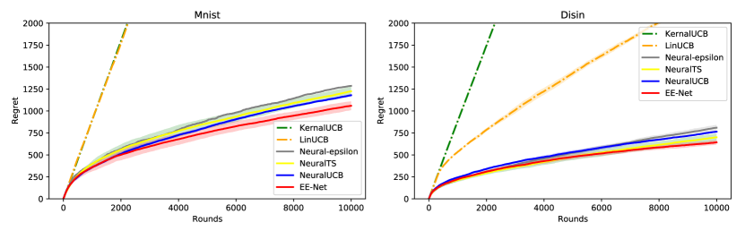
(a) Regret comparison on Mnist and Disin (mean of 10 runs with standard deviation (shadow)).

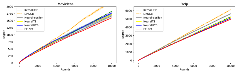
(b) Regret comparison on Movielens and Yelp (average of 10 runs with standard deviation (shadow)).

Figure 2: With the same exploitation network $f_{1}$, EE-Net outperforms all baselines.

Results. Table 2 reports the average cumulative regrets of all methods in 10000 rounds. Figure 2(a) and Figure 2(b) show the regret comparison on these four datasets. EE-Net consistently outperforms all baselines across all datasets. For LinUCB and KernelUCB, the simple linear reward function or predefined kernel cannot properly formulate the ground-truth reward function existing in real-world datasets. In particular, on Mnist and Disin datasets, the correlations between rewards and arm feature vectors are not linear or some simple mappings. Thus, LinUCB and KernelUCB barely exploit the past collected data samples and fail to select the optimal arms. For neural-based bandit algorithms, the exploration probability of Neural-Epsilon is fixed and difficult to adjust. Thus it is usually hard to make effective exploration. To make exploration, NeuralUCB statistically calculates a gradient-based upper confidence bound and NeuralTS draws each arm’s predicted reward from a normal distribution where the standard deviation is computed by gradient. However, the confidence bound or standard deviation they calculate only considers the worst cases and thus may not be able represent the actual potential of each arm, and they cannot make "upward" and "downward" exploration properly. Instead, EE-Net uses a neural network $f_{2}$ to learn each arm’s potential by neural network’s powerful representation ability. Therefore, EE-Net can outperform these two state-of-the-art bandit algorithms. Note that NeuralUCB/TS does need two parameters to tune UCB/TS according to different scenarios while EE-Net only needs to set up a neural network and automatically learns it.

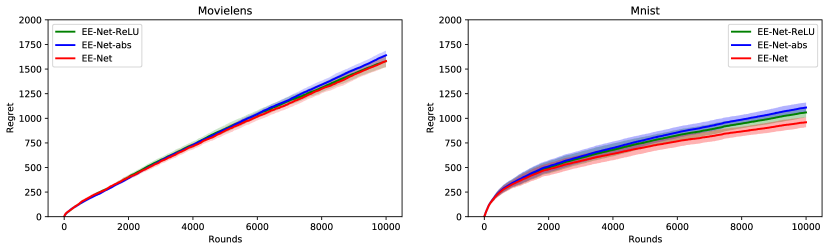
Figure 3: Ablation study on label function $y$ for $f_{2}$. EE-Net denotes $y_{1}=r-f_{1}$, EE-Net-abs denotes $y_{2}=|r-f_{1}|$, and EE-Net-ReLU denotes $y_{3}=\text{ReLU}(r-f_{1})$. EE-Net shows the best performance on these two datasets.

Ablation Study for $y$. In this paper, we use $y_{1}=r-f_{1}$ to measure the potential gain of an arm, as the label of $f_{2}$. Moreover, we provide other two intuitive form $y_{2}=|r-f_{1}|$ and $y_{3}=\text{ReLU}(r-f_{1})$. Figure 3 shows the regret with different $y$, where "EE-Net" denotes our method with default $y_{1}$, "EE-Net-abs" represents the one with $y_{2}$ and "EE-Net-ReLU" is with $y_{3}$. On Movielens and Mnist datasets, EE-Net slightly outperforms EE-Net-abs and EE-Net-ReLU. In fact, $y_{1}$ can effectively represent the positive potential gain and negative potential gain, such that $f_{2}$ intends to score the arm with positive gain higher and score the arm with negative gain lower. However, $y_{2}$ treats the positive/negative potential gain evenly, weakening the discriminative ability. $y_{3}$ can recognize the positive gain while neglecting the difference of negative gain. Therefore, $y_{1}$ usually is the most effective one for empirical performance.

7 Conclusion

In this paper, we propose a novel exploration strategy, EE-Net, by investigating the exploration direction in contextual bandits. In addition to a neural network that exploits collected data in past rounds, EE-Net has another neural network to learn the potential gain compared to the current estimate for adaptive exploration. We provide an instance-dependent regret upper bound for EE-Net and then use experiments to demonstrate its empirical performance.

Appendix A Further Discussion

A.1 Independence of Input or Effective Dimension

This property comes from the new analysis methodology of EE-Net. As the linear bandits (Gentile et al., 2014; Li et al., 2016; Gentile et al., 2017; Li et al., 2019;) work in the Euclidean space and build the confidence ellipsoid for $\boldsymbol{\theta}^{\ast}$ (optimal parameters) based on the linear function $\mathbb{E}[r_{t,i}\mid\mathbf{x}_{t,i}]=\langle\mathbf{x}_{t,i},\boldsymbol{\theta}^{\ast}\rangle$, their regret bounds contain $d$ because $\mathbf{x}_{t,i}\in\mathbb{R}^{d}$. Similarly, neural bandits (Zhou et al., 2020; Zhang et al., 2021) work in the RKHS and construct the confidence ellipsoid for $\boldsymbol{\theta}^{\ast}$ (neural parameters) according to the linear function $\mathbb{E}[r_{t,i}\mid\mathbf{x}_{t,i}]=\langle\nabla_{\boldsymbol{\theta}_{0}}f(\mathbf{x}_{t,i};\boldsymbol{\theta}_{0}),\boldsymbol{\theta}^{\ast}-\boldsymbol{\theta}_{0}\rangle$, where $\nabla_{\boldsymbol{\theta}_{0}}f(\mathbf{x}_{t,i};\boldsymbol{\theta}_{0})\in\mathbb{R}^{\tilde{d}}$. Their analysis is built on the NTK approximation, which is a linear approximation with respect to the gradient. Thus their regret bounds are affected by $\tilde{d}$ due to $\nabla_{\boldsymbol{\theta}_{0}}f(\mathbf{x}_{t,i};\boldsymbol{\theta}_{0})\in\mathbb{R}^{\tilde{d}}$. On the contrary, our analysis is based on the convergence error (regression) and generalization bound of the neural networks. The convergence error term is controlled by the complexity term $\Psi^{\ast}$. And the generalization bound is the standard large-deviation bound, which depends on the number of data points (rounds). These two terms are both independent of $d$ and $\tilde{d}$, which paves the way for our approach to removing both $d$ and $\tilde{d}$ (Lemma 5.1).

A.2 Motivation of Exploration Network

Table 3: Selection Criterion Comparison ($\mathbf{x}_{t}$: selected arm in round $t$).

Methods	Selection Criterion
Neural Epsilon-greedy	With probability $1-\epsilon$, $\mathbf{x}_{t}=\arg\max_{\mathbf{x}_{t,i},i\in[n]}f_{1}(\mathbf{x}_{t,i};\boldsymbol{\theta}^{1})$; Otherwise, select $\mathbf{x}_{t}$ randomly.
NeuralTS (Zhang et al., 2021)	For $\mathbf{x}_{t,i},\forall i\in[n]$, draw $\hat{r}_{t,i}$ from $\mathcal{N}(f_{1}(\mathbf{x}_{t,i};\boldsymbol{\theta}^{1}),{\sigma_{t,i}}^{2})$. Then, select $\mathbf{x}_{t,\hat{i}}$, $\hat{i}=\arg\max_{i\in[n]}\hat{r}_{t,i}.$
NeuralUCB (Zhou et al., 2020)	$\mathbf{x}_{t}=\arg\max_{\mathbf{x}_{t,i},i\in[n]}\left(f_{1}(\mathbf{x}_{t,i};\boldsymbol{\theta}^{1})+\text{UCB}_{t,i}\right).$
EE-Net (Our approach)	$\forall i\in[n]$, compute $f_{1}(\mathbf{x}_{t,i};\boldsymbol{\theta}^{1})$, $f_{2}\left(\nabla_{\boldsymbol{\theta}^{1}}f_{1}(\mathbf{x}_{t,i};\boldsymbol{\theta}^{1});\boldsymbol{\theta}^{2}\right)$ (Exploration Net). Then $\mathbf{x}_{t}=\arg\max_{\mathbf{x}_{t,i}i\in[n]}f_{3}(f_{1},f_{2};\boldsymbol{\theta}^{3})$.

In this section, we list one gradient-based UCB from existing works (Ban et al., 2021; Zhou et al., 2020), which motivates our design of exploration network $f_{2}$.

Lemma A.1.

(Lemma 5.2 in (Ban et al., 2021)). Given a set of context vectors $\{\mathbf{x}_{t}\}_{t=1}^{T}$ and the corresponding rewards $\{r_{t}\}_{t=1}^{T}$ , $\mathbb{E}(r_{t})=h(\mathbf{x}_{t})$ for any $\mathbf{x}_{t}\in\{\mathbf{x}_{t}\}_{t=1}^{T}$. Let $f(\mathbf{x}_{t};\boldsymbol{\theta})$ be the $L$-layers fully-connected neural network where the width is $m$, the learning rate is $\eta$, the number of iterations of gradient descent is $K$. Then, there exist positive constants $C_{1},C_{2},S$, such that if

$$m \geq\text{poly}(T,n,L,\log(1/\delta)\cdot d\cdot e^{\sqrt{\log 1/\delta}}),\ \ \eta=\mathcal{O}(TmL+m\lambda)^{-1},\ \ K\geq\widetilde{\mathcal{O}}(TL/\lambda),$$

then, with probability at least $1-\delta$, for any $\mathbf{x}_{t,i}$, we have the following upper confidence bound:

$$\left|h(\mathbf{x}_{t,i})-f(\mathbf{x}_{t,i};\boldsymbol{\theta}_{t})\right|\leq \gamma_{1}\|\nabla_{\boldsymbol{\theta}_{t}}f(\mathbf{x}_{t,i};\boldsymbol{\theta}_{t})/\sqrt{m}\|_{\mathbf{A}_{t}^{-1}}+\gamma_{2}+\gamma_{1}\gamma_{3}+\gamma_{4},\$$ (A.1)

where

$$\gamma_{1}(m,L)=(\lambda+t\mathcal{O}(L))\cdot((1-\eta m\lambda)^{J/2}\sqrt{t/\lambda})+1$$

$$\gamma_{2}(m,L,\delta)=\|\nabla_{\boldsymbol{\theta}_{t}}f(\mathbf{x}_{t,i};\boldsymbol{\theta}_{t})/\sqrt{m}\|_{\mathbf{A}_{t}^{{}^{\prime}-1}}\cdot\left(\sqrt{\log\left(\frac{\text{det}(\mathbf{A}_{t}^{\prime})}{\text{det}(\lambda\mathbf{I})}\right)-2\log\delta}+\lambda^{1/2}S\right)$$

$$\gamma_{3}(m,L)=C_{2}m^{-1/6}\sqrt{\log m}t^{1/6}\lambda^{-7/6}L^{7/2},\ \ \gamma_{4}(m,L)=C_{1}m^{-1/6}\sqrt{\log m}t^{2/3}\lambda^{-2/3}L^{3}$$

$$\mathbf{A}_{t}=\lambda\mathbf{I}+\sum_{i=1}^{t}\nabla_{\boldsymbol{\theta}_{t}}f(\mathbf{x}_{t,i};\boldsymbol{\theta}_{t})\nabla_{\boldsymbol{\theta}_{t}}f(\mathbf{x}_{t,i};\boldsymbol{\theta}_{t})^{\intercal}/m,\ \,\mathbf{A}_{t}^{\prime}=\lambda\mathbf{I}+\sum_{i=1}^{t}\nabla_{\boldsymbol{\theta}_{0}}f(\mathbf{x}_{t,i};\boldsymbol{\theta}_{0})\nabla_{\boldsymbol{\theta}_{0}}f(\mathbf{x}_{t,i};\boldsymbol{\theta}_{0})^{\intercal}/m.$$

Note that $g(\mathbf{x}_{t};\boldsymbol{\theta}_{0})$ is the gradient at initialization, which can be initialized as constants. Therefore, the above UCB can be represented as the following form for exploitation network $f_{1}$: $|h(\mathbf{x}_{t,i})-f_{1}(\mathbf{x}_{t,i};\boldsymbol{\theta}^{1}_{t})|\leq g(\nabla_{\boldsymbol{\theta}_{t}}f(\mathbf{x}_{t,i};\boldsymbol{\theta}_{t}))$.

Given an arm $x$, let $f_{1}(x)$ be the estimated reward and $h(x)$ be the expected reward. The exploration network $f_{2}$ in EE-Net is to learn $h(x)-f_{1}(x)$, i.e., the residual between expected reward and estimated reward, which is the ultimate goal of making exploration. There are advantages of using a network $f_{2}$ to learn $h(x)-f_{1}(x)$ in EE-Net, compared to giving a statistical upper bound for it such as NeuralUCB, (Ban et al., 2021), and NeuralTS (in NeuralTS, the variance $\nu$ can be thought of as the upper bound). For EE-Net, the approximation error for $h(x)-f_{1}(x)$ is caused by the genenalization error of the neural network (Lemma B.1. in the manuscript). In contrast, for NeuralUCB, (Ban et al., 2021), and NeuralTS, the approximation error for $h(x)-f_{1}(x)$ includes three parts. The first part is caused by ridge regression. The second part of the approximation error is caused by the distance between ridge regression and Neural Tangent Kernel (NTK). The third part of the approximation error is caused by the distance between NTK and the network function. Because they use the upper bound to make selections, the errors inherently exist in their algorithms. By reducing the three parts of the approximation errors to only the neural network convergence error, EE-Net achieves tighter regret bound compared to them (improving by roughly $\sqrt{\log T}$).

Table 4: Exploration Direction Comparison.

Methods	"Upward" Exploration	"Downward" Exploration
NeuralUCB	$\surd$	$\times$
NeuralTS	Randomly	Randomly
EE-Net	$\surd$	$\surd$

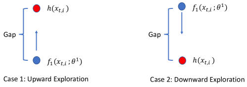
Figure 4: Two types of exploration: Upward exploration and Downward exploration. $f_{1}$ is the exploitation network (estimated reward) and $h$ is the expected reward.

The two types of exploration are described by Figure 4. When the estimated reward is larger than the expected reward, i.e., $h(x)-f_{1}(x)<0$, we need to do the ‘downward exploration’, i.e., lowering the exploration score of $x$ to reduce its chance of being explored; when $h(x)-f_{1}(x)>0$, we should do the ‘upward exploration’, i.e., raising the exploration score of $x$ to increase its chance of being explored. For EE-Net, $f_{2}$ is to learn $h(x)-f_{1}(x)$. When $h(x)-f_{1}(x)>0$, $f_{2}(x)$ will also be positive to make the upward exploration. When $h(x)-f_{1}(x)<0$, $f_{2}(x)$ will be negative to make the downward exploration. In contrast, NeuralUCB will always choose upward exploration, i.e., $f_{1}(x)+CB(x)$ where $CB(x)$ is always positive. In particular, when $h(x)-f_{1}(x)<0$, NeuralUCB will further amplify the mistake. NeuralTS will randomly choose upward or downward exploration for all cases, because it draws a sampled reward from a normal distribution where the mean is $f_{1}(x)$ and the variance $\nu$ is the upper bound.

Appendix B Proof of Theorem 1

B.1 Bounds for Generic Neural Networks

In this section, we provide some base lemmas for the neural networks with respect to gradient or loss. Let $\mathbf{x}_{t}=\mathbf{x}_{t,\widehat{i}}$. Recall that $\mathcal{L}_{t}(\boldsymbol{\theta})=(f(\mathbf{x}_{t};\boldsymbol{\theta})-r_{t})^{2}/2$. Following Allen-Zhu et al. (2019); Cao and Gu (2019), given an instance $\mathbf{x},\|\mathbf{x}\|=1$, we define the outputs of hidden layers of the neural network (Eq. (5.1)):

$$\mathbf{h}_{0}=\mathbf{x},\mathbf{h}_{l}=\sigma(\mathbf{W}_{l}\mathbf{h}_{l-1}),l\in[L-1].$$

Then, we define the binary diagonal matrix functioning as ReLU:

$$\mathbf{D}_{l}=\text{diag}(\mathbbm{1}\{(\mathbf{W}_{l}\mathbf{h}_{l-1})_{1}\},\dots,\mathbbm{1}\{(\mathbf{W}_{l}\mathbf{h}_{l-1})_{m}\}),l\in[L-1],$$

where $\mathbbm{1}$ is the indicator function : $\mathbbm{1}(x)=1$ if $x>0$; $\mathbbm{1}(x)=0$, otherwise. Accordingly, the neural network (Eq. (5.1)) is represented by

$$f(\mathbf{x};\boldsymbol{\theta}^{1}\ \text{or}\ \boldsymbol{\theta}^{2})=\mathbf{W}_{L}(\prod_{l=1}^{L-1}\mathbf{D}_{l}\mathbf{W}_{l})\mathbf{x},$$ (B.1)

and

$$\nabla_{\mathbf{W}_{l}}f=\begin{cases}[\mathbf{h}_{l-1}\mathbf{W}_{L}(\prod_{\tau=l+1}^{L-1}\mathbf{D}_{\tau}\mathbf{W}_{\tau})]^{\top},l\in[L-1]\\ \mathbf{h}_{L-1}^{\top},l=L.\end{cases}$$ (B.2)

Then, we have the following auxiliary lemmas.

Lemma B.1.

Suppose $m,\eta_{1},\eta_{2}$ satisfy the conditions in Theorem 1. With probability at least $1-\mathcal{O}(TnL^{2})\cdot\exp(-\Omega(m\omega^{2/3}L))$ over the random initialization, for all $t\in[T],i\in[n]$, $\boldsymbol{\theta}$ satisfying $\|\boldsymbol{\theta}-\boldsymbol{\theta}_{0}\|_{2}\leq\omega$ with $\omega\leq\mathcal{O}(L^{-9/2}[\log m]^{-3})$, it holds uniformly that

$$(1),|f(\mathbf{x}_{t,i};\boldsymbol{\theta})|\leq\mathcal{O}(1).$$

$$(2),\|\nabla_{\boldsymbol{\theta}}f(\mathbf{x}_{t,i};\boldsymbol{\theta})\|_{2}\leq\mathcal{O}(\sqrt{L}).$$

$$(3),\|\nabla_{\boldsymbol{\theta}}\mathcal{L}_{t}(\boldsymbol{\theta})\|_{2}\leq\mathcal{O}(\sqrt{L})$$

Proof.

(1) is a simply application of Cauchy–Schwarz inequality.

$$|f(\mathbf{x}_{t,i};\boldsymbol{\theta})| =|\mathbf{W}_{L}(\prod_{l=1}^{L-1}\mathbf{D}_{l}\mathbf{W}_{l})\mathbf{x}_{t,i}|$$

$$\leq\underbrace{\|\mathbf{W}_{L}(\prod_{l=1}^{L-1}\mathbf{D}_{l}\mathbf{W}_{l})\|_{2}}_{I_{1}}\|\mathbf{x}_{t,i}\|_{2}$$

$$\leq\mathcal{O}(1)$$

where $I_{1}$ is based on the Lemma B.2 (Cao and Gu, 2019): $I_{1}\leq\mathcal{O}(1)$, and $\|\mathbf{x}_{t,i}\|_{2}=1$.

For (2), it holds uniformly that

$$\|\nabla_{\boldsymbol{\theta}}f(\mathbf{x}_{t,i};\boldsymbol{\theta})\|_{2}=\|\text{vec}(\nabla_{\mathbf{W}_{1}}f)^{\top},\dots,\text{vec}(\nabla_{\mathbf{W}_{L}}f)^{\top}\|_{2}\leq\mathcal{O}(\sqrt{L})$$

where $\|\nabla_{\mathbf{W}_{l}}f\|_{F}\leq\mathcal{O}(1),l\in[L]$ is an application of Lemma B.3 (Cao and Gu, 2019) by removing $\sqrt{m}$.

For (3), we have $\|\nabla_{\boldsymbol{\theta}}\mathcal{L}_{t}(\boldsymbol{\theta})\|_{2}\leq|\mathcal{L}_{t}^{\prime}|\cdot\|\nabla_{\boldsymbol{\theta}}f(\mathbf{x}_{t,i};\boldsymbol{\theta})\|_{2}\leq\mathcal{O}(\sqrt{L})$. ∎

Lemma B.2.

Suppose $m,\eta_{1},\eta_{2}$ satisfy the conditions in Theorem 1. With probability at least $1-\mathcal{O}(TnL^{2})\cdot\exp(-\Omega(m\omega^{2/3}L))$ over the random initialization, for all $\|\mathbf{x}\|_{2}=1$, $\boldsymbol{\theta}$ satisfying $\|\boldsymbol{\theta}-\boldsymbol{\theta}_{0}\|_{2},\|\boldsymbol{\theta}^{\prime}-\boldsymbol{\theta}_{0}\|_{2}\leq\omega$ with $\omega\leq\mathcal{O}(L^{-9/2}[\log m]^{-3})$, it holds uniformly that

$$|f(\mathbf{x};\boldsymbol{\theta})-f(\mathbf{x};\boldsymbol{\theta}^{\prime})-\langle\nabla_{\boldsymbol{\theta}^{\prime}}f(\mathbf{x};\boldsymbol{\theta}^{\prime}),\boldsymbol{\theta}-\boldsymbol{\theta}^{\prime}\rangle|\leq\mathcal{O}(w^{1/3}L^{2}\sqrt{\log m})\|\boldsymbol{\theta}-\boldsymbol{\theta}^{\prime}\|_{2}.$$

Proof.

Based on Lemma 4.1 (Cao and Gu, 2019), it holds uniformly that

$$|\sqrt{m}f(\mathbf{x};\boldsymbol{\theta})-\sqrt{m}f(\mathbf{x};\boldsymbol{\theta}^{\prime})-\langle\sqrt{m}\nabla_{\boldsymbol{\theta}^{\prime}}f(\mathbf{x};\boldsymbol{\theta}^{\prime}),\boldsymbol{\theta}-\boldsymbol{\theta}^{\prime}\rangle|\leq\mathcal{O}(w^{1/3}L^{2}\sqrt{m\log(m)})\|\boldsymbol{\theta}-\boldsymbol{\theta}^{\prime}\|_{2},$$

where $\sqrt{m}$ comes from the different scaling of neural network structure. Removing $\sqrt{m}$ completes the proof. ∎

Lemma B.3.

Suppose $m,\eta_{1},\eta_{2}$ satisfy the conditions in Theorem 1. With probability at least $1-\mathcal{O}(TnL^{2})\cdot\exp(-\Omega(m\omega^{2/3}L))$ over the random initialization, for all $t\in[T],i\in[n]$, $\boldsymbol{\theta},\boldsymbol{\theta}^{\prime}\in B(\boldsymbol{\theta}_{0},\omega)$ with $\omega\leq\mathcal{O}(L^{-9/2}[\log m]^{-3})$, it holds uniformly that

$$|f(\mathbf{x}_{t,i};\boldsymbol{\theta})-f(\mathbf{x}_{t,i};\boldsymbol{\theta}^{\prime})|\leq \mathcal{O}(\omega\sqrt{L})+\mathcal{O}(\omega^{4/3}L^{2}\sqrt{\log m})$$ (B.3)

Proof.

Based on Lemma B.2, we have

$$|f(\mathbf{x}_{t,i};\boldsymbol{\theta})-f(\mathbf{x}_{t,i};\boldsymbol{\theta}^{\prime})|$$

$$\overset{(a)}{\leq} |\langle\nabla_{\boldsymbol{\theta}^{\prime}}f(\mathbf{x}_{t,i};\boldsymbol{\theta}^{\prime}),\boldsymbol{\theta}-\boldsymbol{\theta}^{\prime}\rangle|+\mathcal{O}(\omega^{1/3}L^{2}\sqrt{\log m})\|\boldsymbol{\theta}-\boldsymbol{\theta}^{\prime}\|_{2}$$

$$\overset{(b)}{\leq} \|\nabla_{\boldsymbol{\theta}^{\prime}}f(\mathbf{x}_{t,i};\boldsymbol{\theta}^{\prime})\|_{2}\cdot\|\boldsymbol{\theta}-\boldsymbol{\theta}^{\prime}\|_{2}+\mathcal{O}(\omega^{1/3}L^{2}\sqrt{\log m})\|\boldsymbol{\theta}-\boldsymbol{\theta}^{\prime}\|_{2}$$

$$\overset{(c)}{\leq} \mathcal{O}(\sqrt{L})\|\boldsymbol{\theta}-\boldsymbol{\theta}^{\prime}\|_{2}+\mathcal{O}(\omega^{1/3}L^{2}\sqrt{\log m})\|\boldsymbol{\theta}-\boldsymbol{\theta}^{\prime}\|_{2}$$

$$\leq \mathcal{O}(\omega\sqrt{L})+\mathcal{O}(\omega^{4/3}L^{2}\sqrt{\log m}),$$

where (a) is an application of Lemma B.2, (b) is based on the Cauchy–Schwarz inequality, and (c) is due to Lemma B.1. The proof is completed. ∎

Lemma B.4 (Almost Convexity of Loss).

Let $\mathcal{L}_{t}(\boldsymbol{\theta})=(f(\mathbf{x}_{t};\boldsymbol{\theta})-r_{t})^{2}/2$. Suppose $m,\eta_{1},\eta_{2}$ satisfy the conditions in Theorem 1. With probability at least $1-\mathcal{O}(TnL^{2})\exp[-\Omega(m\omega^{2/3}L)]$ over randomness, for all $t\in[T],i\in[n]$, and $\boldsymbol{\theta},\boldsymbol{\theta}^{\prime}$ satisfying $\|\boldsymbol{\theta}-\boldsymbol{\theta}_{0}\|_{2}\leq\omega$ and $\|\boldsymbol{\theta}^{\prime}-\boldsymbol{\theta}_{0}\|_{2}\leq\omega$ with $\omega\leq\mathcal{O}(L^{-6}[\log m]^{-3/2})$, it holds uniformly that

$$\mathcal{L}_{t}(\boldsymbol{\theta}^{\prime})\geq\mathcal{L}_{t}(\boldsymbol{\theta})+\langle\nabla_{\boldsymbol{\theta}}\mathcal{L}_{t}(\boldsymbol{\theta}),\boldsymbol{\theta}^{\prime}-\boldsymbol{\theta}\rangle-\epsilon.$$

where $\epsilon=\mathcal{O}(\omega^{4/3}L^{3}\sqrt{\log m}))$

Proof.

Let $\mathcal{L}_{t}^{\prime}$ be the derivative of $\mathcal{L}_{t}$ with respective to $f(\mathbf{x}_{t,i};\boldsymbol{\theta})$. Then, it holds that $|\mathcal{L}_{t}^{\prime}|\leq\mathcal{O}(1)$ based on Lemma B.1. Then, by convexity of $\mathcal{L}_{t}$, we have

$$\mathcal{L}_{t}(\boldsymbol{\theta}^{\prime})-\mathcal{L}_{t}(\boldsymbol{\theta})$$

$$\overset{(a)}{\geq} \mathcal{L}_{t}^{\prime}[f(\mathbf{x}_{t,i};\boldsymbol{\theta}^{\prime})-f(\mathbf{x}_{t,i};\boldsymbol{\theta})]$$

$$\overset{(b)}{\geq} \mathcal{L}_{t}^{\prime}\langle\nabla f(\mathbf{x}_{t,i};\boldsymbol{\theta}),\boldsymbol{\theta}^{\prime}-\boldsymbol{\theta}\rangle$$

$$-|\mathcal{L}_{t}^{\prime}|\cdot|f(\mathbf{x}_{t,i};\boldsymbol{\theta}^{\prime})-f(\mathbf{x}_{t,i};\boldsymbol{\theta})-\langle\nabla f(\mathbf{x}_{t,i};\boldsymbol{\theta}),\boldsymbol{\theta}^{\prime}-\boldsymbol{\theta}\rangle|$$

$$\geq \langle\nabla_{\boldsymbol{\theta}}\mathcal{L}_{t}(\boldsymbol{\theta}),\boldsymbol{\theta}^{\prime}-\boldsymbol{\theta}\rangle-|\mathcal{L}_{t}^{\prime}|\cdot|f(\mathbf{x}_{t,i};\boldsymbol{\theta}^{\prime})-f(\mathbf{x}_{t,i};\boldsymbol{\theta})-\langle\nabla f(\mathbf{x}_{t,i};\boldsymbol{\theta}),\boldsymbol{\theta}^{\prime}-\boldsymbol{\theta}\rangle|$$

$$\overset{(c)}{\geq} \langle\nabla_{\boldsymbol{\theta}^{\prime}}\mathcal{L}_{t},\boldsymbol{\theta}^{\prime}-\boldsymbol{\theta}\rangle-\mathcal{O}(\omega^{4/3}L^{3}\sqrt{\log m}))$$

$$.\geq \langle\nabla_{\boldsymbol{\theta}^{\prime}}\mathcal{L}_{t},\boldsymbol{\theta}^{\prime}-\boldsymbol{\theta}\rangle-\epsilon$$

where $(a)$ is due to the convexity of $\mathcal{L}_{t}$, $(b)$ is an application of triangle inequality, and $(c)$ is the application of Lemma B.2. The proof is completed. ∎

Lemma B.5 (Trajectory Ball).

Suppose $m,\eta_{1},\eta_{2}$ satisfy the conditions in Theorem 1. With probability at least $1-\mathcal{O}(TnL^{2})\exp[-\Omega(m\omega^{2/3}L)]$ over randomness of $\boldsymbol{\theta}_{0}$, for any $R>0$, it holds uniformly that

$$\|\boldsymbol{\theta}_{t}^{1}-\boldsymbol{\theta}_{0}\|_{2}\leq\mathcal{O}(R/m^{1/4})\ \&\ \|\boldsymbol{\theta}_{t}^{2}-\boldsymbol{\theta}_{0}\|_{2}\leq\mathcal{O}(R/m^{1/4}),t\in[T].$$

Proof.

Let $\omega=\Omega(R/m^{1/4})$. The proof follows a simple induction. Obviously, $\boldsymbol{\theta}_{0}$ is in $B(\boldsymbol{\theta}_{0},\omega)$. Suppose that $\boldsymbol{\theta}_{1},\boldsymbol{\theta}_{2},\dots,\boldsymbol{\theta}_{T}\in\mathcal{B}(\boldsymbol{\theta}_{0}^{2},\omega)$. We have, for any $t\in[T]$,

$$\|\boldsymbol{\theta}_{T}-\boldsymbol{\theta}_{0}\|_{2} \leq\sum_{t=1}^{T}\|\boldsymbol{\theta}_{t}-\boldsymbol{\theta}_{t-1}\|_{2}\leq\sum_{t=1}^{T}\eta\|\nabla\mathcal{L}_{t}(\boldsymbol{\theta}_{t-1})\|\leq\sum_{t=1}^{T}\eta\mathcal{O}(\sqrt{L})$$

$$=\mathcal{O}(TR^{2}\sqrt{L}/\sqrt{m})\leq\mathcal{O}(R/m^{1/4})$$

The proof is completed. ∎

Theorem 2 (Instance-dependent Loss Bound).

Let $\mathcal{L}_{t}(\boldsymbol{\theta})=(f(\mathbf{x}_{t,\widehat{i}};\boldsymbol{\theta})-r_{t,\widehat{i}})^{2}/2$. Suppose $m,\eta_{1},\eta_{2}$ satisfy the conditions in Theorem 1. With probability at least $1-\mathcal{O}(TnL^{2})\exp[-\Omega(m\omega^{2/3}L)]$ over randomness of $\boldsymbol{\theta}_{0}^{2}$, given any $R>0$ it holds that

$$\sum_{t=1}^{T}\mathcal{L}_{t}(\boldsymbol{\theta}_{t-1}^{2})\leq\sum_{t=1}^{T}\mathcal{L}_{t}(\boldsymbol{\theta}^{\ast})+\mathcal{O}(1)+\frac{TLR^{2}}{\sqrt{m}}+\mathcal{O}(\frac{TR^{4/3}L^{2}\sqrt{\log m}}{m^{1/3}}).$$ (B.4)

where $\boldsymbol{\theta}^{\ast}=\arg\inf_{\boldsymbol{\theta}\in B(\boldsymbol{\theta}_{0}^{2},R/m^{1/4})}\sum_{t=1}^{T}\mathcal{L}_{t}(\boldsymbol{\theta})$.

Proof.

Let $\boldsymbol{\theta}^{\prime}\in B(\boldsymbol{\theta}_{0}^{2},R/m^{1/4})$. In round $t$, based on Lemma B.5, for all $t\in[T]$, $\|\boldsymbol{\theta}_{t}-\boldsymbol{\theta}^{\prime}\|_{2}\leq\omega=\Omega(R/m^{1/4})$, it holds uniformly,

$$\mathcal{L}_{t}(\boldsymbol{\theta}_{t-1}^{2})-\mathcal{L}_{t}(\boldsymbol{\theta}^{\prime})\leq \langle\nabla\mathcal{L}_{t}(\boldsymbol{\theta}_{t-1}^{2}),\boldsymbol{\theta}_{t-1}^{2}-\boldsymbol{\theta}^{\prime}\rangle+\epsilon,$$

where $\epsilon=O(\omega^{4/3}L^{2}\sqrt{\log m})$.

Therefore, for all $t\in[T],\boldsymbol{\theta}^{\prime}\in B(\boldsymbol{\theta}_{0}^{2},R/m^{1/4})$, it holds uniformly

$$\mathcal{L}_{t}(\boldsymbol{\theta}_{t-1}^{2})-\mathcal{L}_{t}(\boldsymbol{\theta}^{\prime})\overset{(a)}{\leq} \frac{\langle\boldsymbol{\theta}_{t-1}^{2}-\boldsymbol{\theta}_{t}^{2},\boldsymbol{\theta}_{t-1}^{2}-\boldsymbol{\theta}^{\prime}\rangle}{\eta_{2}}+\epsilon~{}$$

$$\overset{(b)}{=} \frac{\|\boldsymbol{\theta}_{t-1}^{2}-\boldsymbol{\theta}^{\prime}\|_{2}^{2}+\|\boldsymbol{\theta}_{t-1}^{2}-\boldsymbol{\theta}_{t}^{2}\|_{2}^{2}-\|\boldsymbol{\theta}_{t}^{2}-\boldsymbol{\theta}^{\prime}\|_{2}^{2}}{2\eta_{2}}+\epsilon~{}$$

$$\overset{(c)}{\leq} \frac{\|\boldsymbol{\theta}_{t-1}^{2}-\boldsymbol{\theta}^{\prime}\|_{2}^{2}-\|\boldsymbol{\theta}_{t}^{2}-\boldsymbol{\theta}^{\prime}\|_{2}^{2}}{2\eta_{2}}+O(L\eta_{2})+\epsilon$$

where $(a)$ is because of the definition of gradient descent, $(b)$ is due to the fact $2\langle A,B\rangle=\|A\|^{2}_{F}+\|B\|_{F}^{2}-\|A-B\|_{F}^{2}$, $(c)$ is by $\|\boldsymbol{\theta}_{t-1}^{2}-\boldsymbol{\theta}_{t}^{2}\|^{2}_{2}=\|\eta_{2}\nabla_{\boldsymbol{\theta}^{2}_{t-1}}\mathcal{L}_{t}(\boldsymbol{\theta}_{t-1}^{2})\|^{2}_{2}\leq\mathcal{O}(\eta_{2}^{2}L)$.

Then, for $T$ rounds, we have

$$\sum_{t=1}^{T}\mathcal{L}_{t}(\boldsymbol{\theta}_{t-1})-\sum_{t=1}^{T}\mathcal{L}_{t}(\boldsymbol{\theta}^{\prime})$$

$$\overset{(a)}{\leq} \frac{\|\boldsymbol{\theta}_{0}^{2}-\boldsymbol{\theta}^{\prime}\|_{2}^{2}}{2\eta_{2}}+\sum_{t=2}^{T}\|\boldsymbol{\theta}_{t-1}^{2}-\boldsymbol{\theta}^{\prime}\|_{2}^{2}(\frac{1}{2\eta_{2}}-\frac{1}{2\eta_{2}})+\sum_{t=1}^{T}L\eta_{2}+T\epsilon$$

$$\leq \frac{\|\boldsymbol{\theta}_{0}^{2}-\boldsymbol{\theta}^{\prime}\|_{2}^{2}}{2\eta_{2}}+\sum_{t=1}^{T}L\eta_{2}+T\epsilon$$

$$\overset{(b)}{\leq} \mathcal{O}(\frac{R^{2}}{\sqrt{m}\eta_{2}})+\sum_{t=1}^{T}L\eta_{2}+T\epsilon$$

$$\overset{(c)}{\leq} \mathcal{O}(1)+\frac{TLR^{2}}{\sqrt{m}}+\mathcal{O}(\frac{TR^{4/3}L^{2}\sqrt{\log m}}{m^{1/3}})$$

where $(a)$ is by simply discarding the last term and $(b)$ is because both $\boldsymbol{\theta}^{2}_{0}$ and $\boldsymbol{\theta}^{\prime}$ are in the ball $B(\boldsymbol{\theta}^{2}_{0},R/m^{1/4})$, and $(c)$ is by $\eta_{2}=\frac{R^{2}}{\sqrt{m}}$ and replacing $\epsilon$ with $\omega=\mathcal{O}(R/m^{1/4})$. The proof is completed. ∎

B.2 Exploration Error Bound

See 5.1

Proof.

First, according to Lemma B.5, $\boldsymbol{\theta}^{2}_{0},\dots,\boldsymbol{\theta}_{T-1}^{2}$ all are in $\mathcal{B}(\boldsymbol{\theta}_{0},R/m^{1/4})$. Then, according to Lemma B.1, for any $\mathbf{x}\in\mathbb{R}^{d},\|\mathbf{x}\|_{2}=1$, it holds uniformly $|f_{1}(\mathbf{x}_{t,\widehat{i}};\boldsymbol{\theta}^{1}_{t})+f_{2}(\phi(\mathbf{x}_{t,\widehat{i}});\boldsymbol{\theta}^{2}_{t})-r_{t,\widehat{i}}|\leq\mathcal{O}(1)$.

Then, for any $\tau\in[t]$, define

$$V_{\tau}:= \underset{r_{\tau,\widehat{i}}}{\mathbb{E}}\left[|f_{2}(\phi(\mathbf{x}_{\tau,\widehat{i}});\boldsymbol{\theta}^{2}_{\tau-1})-(r_{\tau,\widehat{i}}-f_{1}(\mathbf{x}_{\tau,\widehat{i}};\boldsymbol{\theta}^{1}_{\tau-1}))|\right]$$ (B.5)

$$-|f_{2}(\phi(\mathbf{x}_{\tau,\widehat{i}});\boldsymbol{\theta}^{2}_{\tau-1})-(r_{\tau,\widehat{i}}-f_{1}(\mathbf{x}_{\tau,\widehat{i}};\boldsymbol{\theta}^{1}_{\tau-1}))|$$

Then, we have

$$\mathbb{E}[V_{\tau}|F_{\tau-1}]= \underset{r_{\tau,\widehat{i}}}{\mathbb{E}}\left[|f_{2}(\phi(\mathbf{x}_{\tau,\widehat{i}});\boldsymbol{\theta}^{2}_{\tau-1})-(r_{\tau,\widehat{i}}-f_{1}(\mathbf{x}_{\tau,\widehat{i}};\boldsymbol{\theta}^{1}_{\tau-1}))|\right]$$ (B.6)

$$-\underset{r_{\tau,\widehat{i}}}{\mathbb{E}}\left[|f_{2}(\phi(\mathbf{x}_{\tau,\widehat{i}});\boldsymbol{\theta}^{2}_{\tau-1})-(r_{\tau,\widehat{i}}-f_{1}(\mathbf{x}_{\tau,\widehat{i}};\boldsymbol{\theta}^{1}_{\tau-1}))\right]$$

$$= 0$$

where $F_{\tau-1}$ denotes the $\sigma$-algebra generated by the history $\mathcal{H}_{\tau-1}$.

Therefore, the sequence $\{V_{\tau}\}_{\tau=1}^{t}$ is the martingale difference sequence. Applying the Hoeffding-Azuma inequality, with probability at least $1-\delta$, we have

$$\mathbb{P}\left[\frac{1}{t}\sum_{\tau=1}^{t}V_{\tau}-\underbrace{\frac{1}{t}\sum_{\tau=1}^{t}\underset{r_{i,\widehat{i}}}{\mathbb{E}}[V_{\tau}|\mathbf{F}_{\tau-1}]}_{I_{1}}>\sqrt{\frac{2\log(1/\delta)}{t}}\right]\leq\delta\\$$ (B.7)

As $I_{1}$ is equal to $0$, we have

$$\frac{1}{t}\sum_{\tau=1}^{t}\underset{r_{\tau,\widehat{i}}}{\mathbb{E}}\left[\left|f_{2}(\phi(\mathbf{x}_{\tau,\widehat{i}});\boldsymbol{\theta}^{2}_{\tau-1})-(r_{\tau,\widehat{i}}-f_{1}(\mathbf{x}_{\tau,\widehat{i}};\boldsymbol{\theta}^{1}_{\tau-1}))\right|\right]$$ (B.8)

$$\leq \underbrace{\frac{1}{t}\sum_{\tau=1}^{t}\left|f_{2}(\phi(\mathbf{x}_{\tau,\widehat{i}});\boldsymbol{\theta}_{\tau-1}^{2})-(r_{\tau,\widehat{i}}-f_{1}(\mathbf{x}_{\tau,\widehat{i}};\boldsymbol{\theta}_{\tau-1}^{1}))\right|}_{I_{3}}+\sqrt{\frac{2\log(1/\delta)}{t}}~{}.$$

For $I_{3}$, based on Theorem 2, for any $\boldsymbol{\theta}^{\prime}$ satisfying $\|\boldsymbol{\theta}^{\prime}-\boldsymbol{\theta}^{2}_{0}\|_{2}\leq R/m^{1/4}$, with probability at least $1-\delta$, we have

$$I_{3} \leq\frac{1}{t}\sqrt{t}\sqrt{\sum_{\tau=1}^{t}\left(f_{2}(\phi(\mathbf{x}_{\tau,\widehat{i}});\boldsymbol{\theta}^{2}_{\tau-1})-(r_{\tau,\widehat{i}}-f_{1}(\mathbf{x}_{\tau,\widehat{i}};\boldsymbol{\theta}_{\tau-1}^{1}))\right)^{2}}$$ (B.9)

$$\leq\frac{1}{t}\sqrt{t}\sqrt{\sum_{\tau=1}^{t}\left(f_{2}(\phi(\mathbf{x}_{\tau,\widehat{i}});\boldsymbol{\theta}^{\prime})-(r_{\tau,\widehat{i}}-f_{1}(\mathbf{x}_{\tau,\widehat{i}};\boldsymbol{\theta}_{\tau-1}^{1}))\right)^{2}}+\frac{\mathcal{O}(1)}{\sqrt{t}}$$

$$\overset{(a)}{\leq}\frac{\sqrt{\Psi(\boldsymbol{\theta}^{2}_{0},R/m^{1/4})}+\mathcal{O}(1)}{\sqrt{t}}.$$

where $(a)$ is based on the definition of instance-dependent complexity term. Combining the above inequalities together, with probability at least $1-\delta$, we have

$$\frac{1}{t}\sum_{\tau=1}^{t}\underset{r_{\tau,\widehat{i}}}{\mathbb{E}}\left[\left|f_{2}(\phi(\mathbf{x}_{\tau,\widehat{i}});\boldsymbol{\theta}^{2}_{\tau-1})-(r_{\tau,\widehat{i}}-f_{1}(\mathbf{x}_{\tau,\widehat{i}};\boldsymbol{\theta}^{1}_{\tau-1})\right|\right]$$ (B.10)

$$\leq\frac{\sqrt{\Psi(\boldsymbol{\theta}^{2}_{0},R/m^{1/4})}+\mathcal{O}(1)}{\sqrt{t}}+\sqrt{\frac{2\log(\mathcal{O}(1)/\delta)}{t}}.$$

The proof is completed. ∎

Corollary 3.

Suppose $m,\eta_{1},\eta_{2}$ satisfy the conditions in Theorem 1. For any $t\in[T]$, let

$$i^{\ast}=\arg\max_{i\in[n]}\left[h(\mathbf{x}_{t,i})\right],$$

and $r_{t,i^{\ast}}$ is the corresponding reward, and denote the policy by $\pi^{\ast}$. Let $\boldsymbol{\theta}^{1,\ast}_{t-1},\boldsymbol{\theta}^{2,\ast}_{t-1}$ be the intermediate parameters trained by Algorithm 1 using the data select by $\pi^{\ast}$. Then, with probability at least $(1-\delta)$ over the random of the initialization, for any $\delta\in(0,1),R>0$, it holds that

$$\frac{1}{t}\sum_{\tau=1}^{t}\underset{r_{\tau,i^{\ast}}}{\mathbb{E}} \left[\left|f_{2}(\phi(\mathbf{x}_{\tau,i^{\ast}});\boldsymbol{\theta}_{\tau-1}^{2,\ast})-\left(r_{\tau,i^{\ast}}-f_{1}(\mathbf{x}_{\tau,i^{\ast}};\boldsymbol{\theta}_{\tau-1}^{1,\ast})\right)\right|\mid\pi^{\ast},\mathcal{H}_{\tau-1}^{\ast}\right]$$ (B.11)

$$\qquad\qquad\leq\frac{\sqrt{\Psi(\boldsymbol{\theta}^{2}_{0},R/m^{1/4})}+\mathcal{O}(1)}{\sqrt{t}}+\sqrt{\frac{2\log(\mathcal{O}(1)/\delta)}{t}},$$

where $\mathcal{H}_{\tau-1}^{\ast}=\{\mathbf{x}_{\tau,i^{\ast}},r_{\tau,i^{\ast}}\}_{\tau^{\prime}=1}^{\tau-1}$ represents the historical data produced by $\pi^{\ast}$ and the expectation is taken over the reward.

Proof.

This a direct corollary of Lemma 5.1, given the optimal historical pairs $\{\mathbf{x}_{\tau,i^{\ast}},r_{\tau,i^{\ast}}\}_{\tau=1}^{t-1}$ according to $\pi^{\ast}$. For brevity, let $f_{2}(\phi(\mathbf{x});\boldsymbol{\theta}_{\tau}^{2,\ast})$ represent $f_{2}\left(\nabla_{\boldsymbol{\theta}^{1,\ast}_{\tau}}f_{1}(\mathbf{x};\boldsymbol{\theta}_{\tau}^{1,\ast});\boldsymbol{\theta}_{\tau}^{2,\ast}\right)$.

Suppose that, for each $\tau\in[t-1]$, $\boldsymbol{\theta}_{\tau}^{1,\ast}$ and $\boldsymbol{\theta}_{\tau}^{2,\ast}$ are the parameters training on $\{\mathbf{x}_{\tau^{\prime}}^{\ast},r_{\tau^{\prime}}^{\ast}\}_{\tau^{\prime}=1}^{\tau}$ according to Algorithm 1 according to $\pi^{\ast}$. Note that these pairs $\{\mathbf{x}_{\tau^{\prime}}^{\ast},r_{\tau^{\prime}}^{\ast}\}_{\tau^{\prime}=1}^{\tau}$ are unknown to the algorithm we run, and the parameters $(\boldsymbol{\theta}_{\tau}^{1,\ast},\boldsymbol{\theta}_{\tau}^{2,\ast})$ are not estimated. However, for the analysis, it is sufficient to show that there exist such parameters so that the conditional expectation of the error can be bounded.

Then, we define

$$V_{\tau} :=\underset{r_{\tau,i^{\ast}}}{\mathbb{E}}\left[\left|f_{2}(\phi(\mathbf{x}_{\tau,i^{\ast}});\boldsymbol{\theta}_{\tau-1}^{2,\ast})-\left(r_{\tau,i^{\ast}}-f_{1}(\mathbf{x}_{\tau,i^{\ast}};\boldsymbol{\theta}_{\tau-1}^{1,\ast})\right)\right|\right]$$ (B.12)

$$\qquad\qquad-\left|f_{2}(\phi(\mathbf{x}_{\tau,i^{\ast}});\boldsymbol{\theta}_{\tau-1}^{2,\ast})-\left(r_{\tau,i^{\ast}}-f_{1}(\mathbf{x}_{\tau,i^{\ast}};\boldsymbol{\theta}_{\tau-1}^{1,\ast})\right)\right|~{}.$$

Then, taking the expectation over reward, we have

$$\mathbb{E}[V_{\tau}|\mathbf{F}_{\tau-1}] =\underset{r_{\tau,i^{\ast}}}{\mathbb{E}}\left[\left|f_{2}\left(\phi(\mathbf{x}_{\tau,i^{\ast}});\boldsymbol{\theta}_{\tau-1}^{2,\ast}\right)-\left(r_{\tau,i^{\ast}}-f_{1}(\mathbf{x}_{\tau,i^{\ast}};\boldsymbol{\theta}_{\tau-1}^{1,\ast})\right)\right|\right]$$ (B.13)

$$\quad-\underset{r_{\tau,i^{\ast}}}{\mathbb{E}}\left[\left|f_{2}\left(\phi(\mathbf{x}_{\tau,i^{\ast}});\boldsymbol{\theta}_{\tau-1}^{2,\ast}\right)-\left(r_{\tau,i^{\ast}}-f_{1}(\mathbf{x}_{\tau,i^{\ast}};\boldsymbol{\theta}_{\tau-1}^{1,\ast})\right)\right|\mid\mathbf{F}_{\tau-1}\right]$$

$$=0~{},$$

where $\mathbf{F}_{\tau-1}$ denotes the $\sigma$-algebra generated by the history $\mathcal{H}_{\tau-1}^{\ast}=\{\mathbf{x}_{\tau,i^{\ast}},r_{\tau,i^{\ast}}\}_{\tau^{\prime}=1}^{\tau-1}$.

Therefore, $\{V_{\tau}\}_{\tau=1}^{t}$ is a martingale difference sequence. Similarly to Lemma 5.1, applying the Hoeffding-Azuma inequality to $V_{\tau}$, with probability $1-\delta$, we have

$$\frac{1}{t}\sum_{\tau=1}^{t}\underset{r_{\tau,i^{\ast}}}{\mathbb{E}}\left[\left|f_{2}(\phi(\mathbf{x}_{\tau,i^{\ast}});\boldsymbol{\theta}_{\tau-1}^{2,\ast})-\left(r_{\tau,i^{\ast}}-f_{1}(\mathbf{x}_{\tau,i^{\ast}};\boldsymbol{\theta}_{\tau-1}^{1,\ast})\right)\right|\right]$$ (B.14)

$$\leq \frac{1}{t}\sum_{\tau=1}^{t}\left|f_{2}(\phi(\mathbf{x}_{\tau,i^{\ast}});\boldsymbol{\theta}_{\tau-1}^{2,\ast})-\left(r_{\tau,i^{\ast}}-f_{1}(\mathbf{x}_{\tau,i^{\ast}};\boldsymbol{\theta}_{\tau-1}^{1,\ast})\right)\right|+\sqrt{\frac{2\log(1/\delta)}{t}}$$

$$\leq \frac{1}{t}\sqrt{t}\sqrt{\sum_{\tau=1}^{t}\left(f_{2}(\phi(\mathbf{x}_{\tau,i^{\ast}});\boldsymbol{\theta}^{2,\ast})-\left(r_{\tau,i^{\ast}}-f_{1}(\mathbf{x}_{\tau,i^{\ast}};\boldsymbol{\theta}_{\tau-1}^{1,\ast})\right)\right)^{2}}+\sqrt{\frac{2\log(1/\delta)}{t}}$$

$$\overset{(a)}{\leq} \frac{1}{t}\sqrt{t}\sqrt{\sum_{\tau=1}^{t}\left(f_{2}(\phi(\mathbf{x}_{\tau,i^{\ast}});\boldsymbol{\theta}^{\prime})-\left(r_{\tau,i^{\ast}}-f_{1}(\mathbf{x}_{\tau,i^{\ast}};\boldsymbol{\theta}_{\tau-1}^{1,\ast})\right)\right)^{2}}+\frac{\mathcal{O}(1)}{\sqrt{t}}+\sqrt{\frac{2\log(1/\delta)}{t}}$$

$$\overset{(b)}{\leq} \frac{\sqrt{\Psi(\boldsymbol{\theta}^{2}_{0},R/m^{1/4})}+\mathcal{O}(1)}{\sqrt{t}}+\sqrt{\frac{2\log(1/\delta)}{t}},$$

where $(a)$ is an application of Lemma 2 for all $\boldsymbol{\theta}^{\prime}\in B(\boldsymbol{\theta}_{0}^{2},R/m^{1/4})$ and $(b)$ is based on the definition of instance-dependent complexity term. Combining the above inequalities, the proof is complete. ∎

B.3 Main Proof

In this section, we provide the proof of Theorem 1.

See 1

Proof.

For brevity, let $f(\mathbf{x};\boldsymbol{\theta}_{t-1})=f_{2}\left(\phi(\mathbf{x}));\boldsymbol{\theta}_{t-1}^{2}\right)+f_{1}(\mathbf{x};\boldsymbol{\theta}_{t-1}^{1}).$ Then, the pseudo regret of round $t$ is given by

$$R_{t} =h(\mathbf{x}_{t,i^{\ast}})-h(\mathbf{x}_{t,\widehat{i}})$$ (B.15)

$$=\underset{r_{t,i},i\in[n]}{\mathbb{E}}[r_{t,i^{\ast}}-r_{t,\widehat{i}}]$$

$$=\underset{r_{t,i},i\in[n]}{\mathbb{E}}[r_{t,i^{\ast}}-r_{t,\widehat{i}}]$$

$$=\underset{r_{t,i},i\in[n]}{\mathbb{E}}[r_{t,i^{\ast}}-f(\mathbf{x}_{t,\widehat{i}};\boldsymbol{\theta}_{t-1})+f(\mathbf{x}_{t,\widehat{i}};\boldsymbol{\theta}_{t-1})-r_{t,\widehat{i}}]$$

$$\leq\underset{r_{t,i},i\in[n]}{\mathbb{E}}[\underbrace{r_{t,i^{\ast}}-f(\mathbf{x}_{t,i^{\ast}};\boldsymbol{\theta}_{t-1})+f(\mathbf{x}_{t,\widehat{i}};\boldsymbol{\theta}_{t-1})-f(\mathbf{x}_{t,\widehat{i}};\boldsymbol{\theta}_{t-1})}_{I_{1}}+f(\mathbf{x}_{t,\widehat{i}};\boldsymbol{\theta}_{t-1})/\sqrt{m}-r_{t,\widehat{i}}]$$

$$=\underset{r_{t,i},i\in[n]}{\mathbb{E}}[r_{t,i^{\ast}}-f(\mathbf{x}_{t,i^{\ast}};\boldsymbol{\theta}_{t-1})+f(\mathbf{x}_{t,\widehat{i}};\boldsymbol{\theta}_{t-1})-r_{t,\widehat{i}}]$$

$$\overset{(a)}{=}\underset{r_{t,i},i\in[n]}{\mathbb{E}}[r_{t,i^{\ast}}-f(\mathbf{x}_{t,i^{\ast}};\boldsymbol{\theta}_{t-1}^{\ast})+f(\mathbf{x}_{t,i^{\ast}};\boldsymbol{\theta}_{t-1}^{\ast})-f(\mathbf{x}_{t,i^{\ast}};\boldsymbol{\theta}_{t-1})+f(\mathbf{x}_{t,\widehat{i}};\boldsymbol{\theta}_{t-1})-r_{t,\widehat{i}}]$$

$$\leq\underset{r_{t,i},i\in[n]}{\mathbb{E}}\left[\left|f_{2}\left(\phi(\mathbf{x}_{t,i^{\ast}});\boldsymbol{\theta}_{t-1}^{2,\ast}\right)-\left(r_{t,i^{\ast}}-f_{1}(\mathbf{x}_{t,i^{\ast}};\boldsymbol{\theta}_{t-1}^{1,\ast})\right)\right|\right]$$

$$\ \ \ +\left|f_{2}(\phi(\mathbf{x}_{t,i^{\ast}});\boldsymbol{\theta}_{t-1}^{2,\ast})-f_{2}(\phi(\mathbf{x}_{t,i^{\ast}});\boldsymbol{\theta}^{2}_{t-1})\right|$$

$$\ \ \ +\left|f_{1}(\mathbf{x}_{t,i^{\ast}};\boldsymbol{\theta}_{t-1}^{1,\ast})-f_{1}(\mathbf{x}_{t,i^{\ast}};\boldsymbol{\theta}_{t-1}^{1})\right|$$

$$\ \ \ +\underset{r_{t,i},i\in[n]}{\mathbb{E}}\left[\left|f_{2}(\phi(\mathbf{x}_{t,\widehat{i}});\boldsymbol{\theta}_{t-1}^{2})-\left(r_{t,\widehat{i}}-f_{1}(\mathbf{x}_{t,\widehat{i}};\boldsymbol{\theta}_{t-1}^{1})\right)\right|\right]$$

where $I_{1}$ is because $f(\mathbf{x}_{t,\widehat{i}};\boldsymbol{\theta}_{t-1})=\max_{i\in[n]}f(\mathbf{x}_{t,i};\boldsymbol{\theta}_{t-1})$ and $f(\mathbf{x}_{t,\widehat{i}};\boldsymbol{\theta}_{t-1})-f(\mathbf{x}_{t,i^{\ast}};\boldsymbol{\theta}_{t-1})\geq 0$ and $(a)$ introduces the intermediate parameters $\boldsymbol{\theta}_{t-1}^{\ast}=(\boldsymbol{\theta}_{t-1}^{1,\ast},\boldsymbol{\theta}_{t-1}^{2,\ast})$ for analysis, which will be suitably chosen.

Therefore, we have

$$\mathbf{R}_{T}= \sum_{t=1}^{T}R_{t}$$ (B.16)

$$\leq \sum_{t=1}^{T}\underbrace{\underset{r_{t,i},i\in[n]}{\mathbb{E}}\left[\left|f_{2}(\phi(\mathbf{x}_{t,i^{\ast}});\boldsymbol{\theta}_{t-1}^{2,\ast})-\left(r_{t,i^{\ast}}-f_{1}(\mathbf{x}_{t,i^{\ast}};\boldsymbol{\theta}_{t-1}^{1,\ast})\right)\right|\right]}_{I_{2}}$$

$$\ \ \ +\sum_{t=1}^{T}\underbrace{\left|f_{2}\left(\phi(\mathbf{x}_{t,i^{\ast}});\boldsymbol{\theta}_{t-1}^{2,\ast}\right)-f_{2}\left(\phi(\mathbf{x}_{t,i^{\ast}});\boldsymbol{\theta}^{1}_{t-1}));\boldsymbol{\theta}_{t-1}^{2}\right)\right|}_{I_{3}}$$

$$\ \ \ +\sum_{t=1}^{T}\underbrace{\left|f_{1}(\mathbf{x}_{t,i^{\ast}};\boldsymbol{\theta}_{t-1}^{1,\ast})-f_{1}(\mathbf{x}_{t,i^{\ast}};\boldsymbol{\theta}_{t-1}^{1})\right|}_{I_{4}}$$

$$\ \ \ +\sum_{t=1}^{T}\underbrace{\underset{r_{t,i},i\in[n]}{\mathbb{E}}\left[\left|f_{2}\left(\phi(\mathbf{x}_{t,\widehat{i}});\boldsymbol{\theta}_{t-1}^{2}\right)-\left(r_{t,\widehat{i}}-f_{1}(\mathbf{x}_{t,\widehat{i}};\boldsymbol{\theta}_{t-1}^{1})\right)\right|\right]}_{I_{5}}$$

$$\leq 2\sum_{t=1}^{T}\Big{(}\frac{\sqrt{\Psi(\boldsymbol{\theta}^{2}_{0},R/m^{1/4})}+\mathcal{O}(1)}{\sqrt{T}}+\sqrt{\frac{2\log(\mathcal{O}(1)/\delta)}{T}}\Big{)}$$

$$+2\sum_{t=1}^{T}\Big{(}\mathcal{O}(\sqrt{L}R/m^{1/4})+\mathcal{O}(R^{4/3}L^{2}\sqrt{\log m}/m^{1/3})\Big{)}$$

$$\leq \sum_{t=1}^{T}\Big{(}\frac{2\sqrt{\Psi(\boldsymbol{\theta}^{2}_{0},R/m^{1/4})}+\mathcal{O}(1)}{\sqrt{T}}+2\sqrt{\frac{2\log(\mathcal{O}(1)/\delta)}{T}}\Big{)}$$

$$+\mathcal{O}(\sqrt{L}TR/m^{1/4})+\mathcal{O}(TR^{4/3}L^{2}\sqrt{\log m}/m^{1/3})$$

$$\overset{(b)}{\leq} 2\sqrt{\Psi(\boldsymbol{\theta}^{2}_{0},R/m^{1/4})T}+2\sqrt{2\log(\mathcal{O}(1)/\delta)T}+\mathcal{O}(1)$$

$I_{2}$ and $I_{5}$ is based on Lemma 5.1 and Corollary 3 , i.e., $I_{2},I_{5}\leq\frac{\sqrt{\Psi(\boldsymbol{\theta}^{2}_{0},R/m^{1/4})}+\mathcal{O}(1)}{\sqrt{T}}+\sqrt{\frac{2\log(\mathcal{O}(1)/\delta)}{T}}$ . $I_{3},I_{4}\leq\mathcal{O}(1)$ are based on Lemma B.3, respectively, because both $\boldsymbol{\theta}^{2}_{t-1},\boldsymbol{\theta}^{2,\ast}_{t-1}\in B(\boldsymbol{\theta}_{0}^{2},R/m^{1/4})$ and $\boldsymbol{\theta}^{1}_{t-1},\boldsymbol{\theta}^{1,\ast}_{t-1}\in B(\boldsymbol{\theta}_{0}^{1},R/m^{1/4}).$ $(b)$ is by the proper choice of $m$, i.e., when $m$ is large enough, we have $I_{3},I_{4}\leq\mathcal{O}(1)$.

The proof is completed. ∎

References

- Abbasi-Yadkori et al. (2011) Yasin Abbasi-Yadkori, Dávid Pál, and Csaba Szepesvári. Improved algorithms for linear stochastic bandits. In Advances in Neural Information Processing Systems, pages 2312–2320, 2011.
- Abeille and Lazaric (2017) Marc Abeille and Alessandro Lazaric. Linear thompson sampling revisited. In Artificial Intelligence and Statistics, pages 176–184. PMLR, 2017.
- Agrawal and Goyal (2013) Shipra Agrawal and Navin Goyal. Thompson sampling for contextual bandits with linear payoffs. In International Conference on Machine Learning, pages 127–135. PMLR, 2013.
- Ahmed et al. (2018) Hadeer Ahmed, Issa Traore, and Sherif Saad. Detecting opinion spams and fake news using text classification. Security and Privacy, 1(1):e9, 2018.
- Allen-Zhu et al. (2019) Zeyuan Allen-Zhu, Yuanzhi Li, and Zhao Song. A convergence theory for deep learning via over-parameterization. In International Conference on Machine Learning, pages 242–252. PMLR, 2019.
- Arora et al. (2019) Sanjeev Arora, Simon S Du, Wei Hu, Zhiyuan Li, Russ R Salakhutdinov, and Ruosong Wang. On exact computation with an infinitely wide neural net. In Advances in Neural Information Processing Systems, pages 8141–8150, 2019.
- Auer (2002) Peter Auer. Using confidence bounds for exploitation-exploration trade-offs. Journal of Machine Learning Research, 3(Nov):397–422, 2002.
- Ban and He (2020) Yikun Ban and Jingrui He. Generic outlier detection in multi-armed bandit. In Proceedings of the 26th ACM SIGKDD International Conference on Knowledge Discovery & Data Mining, pages 913–923, 2020.
- Ban and He (2021a) Yikun Ban and Jingrui He. Convolutional neural bandit: Provable algorithm for visual-aware advertising. arXiv preprint arXiv:2107.07438, 2021a.
- Ban and He (2021b) Yikun Ban and Jingrui He. Local clustering in contextual multi-armed bandits. In Proceedings of the Web Conference 2021, pages 2335–2346, 2021b.
- Ban et al. (2021) Yikun Ban, Jingrui He, and Curtiss B Cook. Multi-facet contextual bandits: A neural network perspective. In The 27th ACM SIGKDD Conference on Knowledge Discovery and Data Mining, Virtual Event, Singapore, August 14-18, 2021, pages 35–45, 2021.
- Ban et al. (2022) Yikun Ban, Yuchen Yan, Arindam Banerjee, and Jingrui He. EE-net: Exploitation-exploration neural networks in contextual bandits. In International Conference on Learning Representations, 2022. URL https://openreview.net/forum?id=X_ch3VrNSRg.
- Bubeck et al. (2011) Sébastien Bubeck, Rémi Munos, Gilles Stoltz, and Csaba Szepesvári. X-armed bandits. Journal of Machine Learning Research, 12(5), 2011.
- Cao and Gu (2019) Yuan Cao and Quanquan Gu. Generalization bounds of stochastic gradient descent for wide and deep neural networks. Advances in Neural Information Processing Systems, 32:10836–10846, 2019.
- Chen et al. (2021) Xinyi Chen, Edgar Minasyan, Jason D Lee, and Elad Hazan. Provable regret bounds for deep online learning and control. arXiv preprint arXiv:2110.07807, 2021.
- Chu et al. (2011) Wei Chu, Lihong Li, Lev Reyzin, and Robert Schapire. Contextual bandits with linear payoff functions. In Proceedings of the Fourteenth International Conference on Artificial Intelligence and Statistics, pages 208–214, 2011.
- Dani et al. (2008) Varsha Dani, Thomas P Hayes, and Sham M Kakade. Stochastic linear optimization under bandit feedback. 2008.
- Deng et al. (2009) Jia Deng, Wei Dong, Richard Socher, Li-Jia Li, Kai Li, and Li Fei-Fei. Imagenet: A large-scale hierarchical image database. In 2009 IEEE conference on computer vision and pattern recognition, pages 248–255. Ieee, 2009.
- Du et al. (2019) Simon Du, Jason Lee, Haochuan Li, Liwei Wang, and Xiyu Zhai. Gradient descent finds global minima of deep neural networks. In International Conference on Machine Learning, pages 1675–1685. PMLR, 2019.
- Filippi et al. (2010) Sarah Filippi, Olivier Cappe, Aurélien Garivier, and Csaba Szepesvári. Parametric bandits: The generalized linear case. In Advances in Neural Information Processing Systems, pages 586–594, 2010.