Horizon fluxes of binary black holes in eccentric orbits

Abstract

We compute the rate of change of mass and angular momentum of a black hole, namely tidal heating, in an eccentric orbit. The change is caused due to the tidal field of the orbiting companion. We compute the result for both the spinning and non-spinning black holes in the leading order of the mean motion, namely $\xi$. We demonstrate that the rates get enhanced significantly for nonzero eccentricity. Since eccentricity in a binary evolves with time we also express the results in terms of an initial eccentricity and azimuthal frequency $\xi_{\phi}$. In the process, we developed a prescription that can be used to compute all physical quantities in a series expansion of initial eccentricity, $e_{0}$. These results are computed taking account of the spin of the binary components. The prescription can be used to compute very high-order corrections of initial eccentricity. We use it to find the contribution to eccentricity up to $\mathcal{O}(e_{0}^{5})$ in the spinning binary. We also provide an approximate expression for $\mathcal{O}(e_{0}^{n})$, where $n$ is any odd number. With this, we compute approximate expression for $\mathcal{O}(e_{0}^{7})$ and $\mathcal{O}(e_{0}^{9})$ for non-spinning binary. Using the computed expression of eccentricity, we derived the rate of change of mass and angular momentum of a black hole in terms of initial eccentricity and azimuthal frequency up to $\mathcal{O}(e_{0}^{6})$.

I Introduction

In recent times, the detection of gravitational waves (GWs) from the coalescence of compact binaries by LIGO Aasi et al. (2015) and Virgo Acernese et al. (2015) has opened up a new era of astronomy Abbott et al. (2019a, 2021a). As a result, these observations have motivated General Relativity (GR) tests  Abbott et al. (2019b); Abbott et al. (2019c). The components of the compact binaries observed by LIGO and Virgo are mainly inferred to be either black holes (BHs) or neutron stars (NSs), which is primarily based on the measurements of component masses, population models, and tidal deformability of NSs Cardoso et al. (2017). The merger of two NSs was also observed in the event GW170817 Abbott et al. (2017), and possibly also GW190425 Abbott et al. (2020). More recently, detections of GW200105 and GW200115 Abbott et al. (2021b) were made where it is believed that it is BH-NS binary. However, it remains to be conclusively proven that the heavier objects observed are indeed BHs of GR.

Currently, the existing detectors are continuously being upgraded. Alongside, there are proposals for several next-generation ground-based detectors such as the Einstein telescope Maggiore et al. (2020) and cosmic explorer Reitze et al. (2019). These detectors will be significantly more sensitive detectors. As a result, it will be possible to measure very small features in the signals. Similarly, space-based detectors such as Laser Interferometer Space Antenna (LISA) Amaro-Seoane et al. (2017) are being built. LISA will observe binaries comprising supermassive bodies. These sources will be either very loud or will last very long in the detector for the detector to measure very small features in the signal. Therefore modeling the signals as accurately as possible has become a necessity.

Due to the causal structure, BHs in GR are perfect absorbers that behave as dissipative systems Thorne et al. (1986); Damour (1982); Poisson (2009); Cardoso and Pani (2013). A striking feature of a BH is its horizon, which is a null surface that does not allow energy to escape outward. In the presence of a companion, the tidal field of the companion affects the BH. These tidal effects change BH’s mass, angular momentum, and horizon area. This phenomenon is called tidal heating (TH) Hartle (1973); Hughes (2001); Poisson and Will (1953). If the BH is nonspinning, then energy and angular momentum flow into the BH. However, if the BHs are spinning then they can transfer their rotational energy from the ergoregion out into the orbit due to tidal interactions with their binary companion. Energy exchange via TH backreacts on the binary’s evolution, resulting in a shift in the phase of the GWs emitted by the system. TH of objects such as NSs or horizonless ECOs is comparatively much less due to their lack of a horizon. So, a careful measurement of this phase shift can be used in principle to distinguish BHs from horizonless compact objects Maselli et al. (2018); Datta and Bose (2019); Datta et al. (2020); Datta (2020); Agullo et al. (2021); Chakraborty et al. (2021); Sherf (2021); Datta and Phukon (2021); Sago and Tanaka (2021); Maggio et al. (2021); Sago and Tanaka (2022).

A compact binary coalescence (CBC) consists primarily of three phases - inspiral, merger, and ringdown. The inspiral can be modeled using post-Newtonian (PN) formalism, whereas numerical relativity (NR) simulations are needed to model the merger regime Pretorius (2007). To study the ringdown part of the dynamics, one needs BH perturbation theory techniques Sasaki and Tagoshi (2003) or NR. Tidal heating is relevant in the inspiral and mostly in the late inspiral when the components are closer together making their tidal interactions stronger. In the PN regime, TH can be incorporated into the gravitational waveform by adding the phase and amplitude shift due to this effect into a PN approximant in the time or frequency domain.

In several studies, TH of black holes has been studied analytically or numerically. It has been demonstrated that in the extreme mass ratio inspirals the impact of TH will be significant Datta et al. (2020); Datta and Bose (2019). It has also been pointed out that TH can be used to distinguish between black holes and neutron stars. As a result, this can address the mass gap problem Datta et al. (2021). The observability in the third-generation detectors has been also studied Mukherjee et al. (2022). Since TH depends on the near horizon properties of a black hole, it is expected that any modification to the near horizon physics can lead to significant modification to TH. Therefore, it can be used to test the near-horizon properties of the black holes which may shed light on the quantum nature of gravity.

However, while computing the TH of classical black holes or studying its impact on the observation only the circular orbits have been considered. Currently, we lack a proper computation as well as an understanding of the TH of black holes in a generic orbit. In the current work, we would like to initiate bridging this gap by analytically computing the leading order TH of BHs in an eccentric orbit. We will leave the computation of TH in a generic orbit for the future.

Throughout the article, we will use geometric units, assuming $G=c=1$ except when it will be required to demonstrate the post-Newtonian (PN) order. Latin indices represent spatial indices running from $1$ to $3$.

II Tidal moments for a two-body system

The post-Newtonian environment upto $1.5$PN order can be described by potentials $U_{ext}$, $U^{a}_{ext}$ and $\Psi_{ext}$ as discussed in Ref. Taylor and Poisson (2008). Once these potentials are known the motion of a BH in the barycentric frame $(t,x^{a})$ can be determined Taylor and Poisson (2008). Similarly, the barycentric tidal moments, $\mathcal{E}_{ab}$ and $\mathcal{B}_{ab}$ can be computed from these potentials. TH is directly connected to the tidal moments “perceived” by the BHs, namely $\bar{\mathcal{E}}_{ab}$ and $\bar{\mathcal{B}}_{ab}$. The corresponding transformation equations can be found in Ref. Taylor and Poisson (2008). Note, this prescription is valid for any post-Newtonian environment.

In the current work, we are interested in the post-Newtonian environment of a binary system. Therefore, the external environment is sourced by a single external body. Assuming the external source to be a post-Newtonian monopole of mass $m_{2}$ at position ${\bf z}_{2}$, the external potentials and their derivatives can be expressed in terms of $m_{2}$, the velocity of the body $v^{a}_{2}$, separation $r$ and the direction vector ${\bf n}$. These expressions can be further simplified if represented with respect to separation vector and relative velocity and by identifying the system’s barycenter with the origin of the coordinate system.

For a generic post-Newtonian orbit fixed in a plane, we can identify the plane to be the $x-y$ plane. We then use the polar coordinates $r$ and $\phi$ to describe the orbital motions. In this system ${\bf r}=(r\cos\phi,r\sin\phi,0)$, and all vectors can be resolved in the basis ${\bf n}=(\cos\phi,\sin\phi,0)$, ${\bf\Phi}=(-\sin\phi,\cos\phi,0)$, and ${\bf l}=(0,0,1)$ is the vector normal to the plane. In this system the tidal field can be written as Taylor and Poisson (2008),

$$\begin{split}\mathcal{E}_{ab}=&-\frac{3m_{2}}{r^{3}}{\bf n}_{\langle ab\rangle}-\frac{3m_{2}}{r^{3}}\Big{(}\left[-\frac{3m_{1}^{2}}{2m^{2}}\dot{r}^{2}+2(r\dot{\phi})^{2}-\frac{5m_{1}+6m_{2}}{2r}\right]{\bf n}_{\langle ab\rangle}\\ &-\frac{(2m_{1}+m_{2})m_{2}}{m^{2}}\dot{r}(r\dot{\phi}){\bf n}_{\langle a}{\bf\Phi}_{b\rangle}+(r\dot{\phi})^{2}{\bf\Phi}_{\langle ab\rangle}\Big{)}+\mathcal{O}(c^{-4})\\ \mathcal{B}_{ab}=&-\frac{6m_{2}}{r^{3}}(r\dot{\phi}){\bf l}_{(a}{\bf n}_{b)}+\mathcal{O}(c^{-2}),\end{split}$$ (1)

where $r$ is the interbody distance, $\phi$ is the angular position of the relative orbit in the plane. We use the notation ${\bf n}_{\langle ab\rangle}={\bf n}_{a}{\bf n}_{b}-\frac{1}{3}\delta_{ab}$ and ${\bf\Phi}_{\langle ab\rangle}={\bf\Phi}_{a}{\bf\Phi}_{b}-\frac{1}{3}\delta_{ab}$.

III Application to eccentric orbit

To address the eccentric orbits we will here discuss the quasi-Keplerian formalism first introduced in Refs. Damour and Schaefer (1988); Schäfer and Wex (1993). It provides a solution to the conservative parts of the post-Newtonian (PN) equations of motion. For the current purpose, the orbital variables $(r,\phi)$ and their derivatives as a function of a parametric angle, namely the eccentric anomaly $u$ are required to be known. It can be achieved with quasi-Keplerian formalism. In this section, we will discuss the relevant physics of a binary in an eccentric orbit. This will set the premise for the computation of the rate of change of mass and angular momentum of a black hole as well as the evolution of the eccentricity of an orbit.

There are three angle variables involved in this approach. The angles $u,\,l$, and $v$ are the eccentric, mean, and true anomalies. The geometrical interpretation of these angles has been discussed in Ref. Moore et al. (2016). The semimajor axis of the ellipse is $a_{r}=(M/n^{2})^{1/3}$. The mean motion is defined as, $n\equiv 2\pi/P$ with $P$ being the radial orbital (periastron to periastron) period. The current work focuses on deriving the horizon fluxes in leading order in dimensionless radial angular orbit frequency $\xi=Mn$. We will use this dimensionless variable extensively in the current work since it helps in getting PN expansions.

In the presence of the post-Newtonian terms the orbits are not exact Keplerian ellipses. Their parametric equations for $r,\,\phi,\,\dot{r}$, and $\dot{\phi}$ still take a similar form. However, these relations are much more complicated. These resulting solutions are referred to as quasi-Keplerian. The explicit analytic expressions can be derived from the conservative contributions to the equations of motion. For this, the radiation-reaction contributions to the equations of motion are ignored. These extensions are known to 3PN order Memmesheimer et al. (2004); Konigsdorffer and Gopakumar (2006).

Unlike in the Newtonian case, now three eccentricities $e_{t}$, $e_{r}$, and $e_{\phi}$ are required to describe the orbit instead of one. These eccentricities are related to each other and to the orbital energy and angular momentum Damour et al. (2004); Memmesheimer et al. (2004). The quasi-Keplerian equations also show the well-known periastron precession. We will not show the expressions here for brevity. The expressions can be found in Ref. Moore et al. (2016).

To find the required PN expansions appropriate set of constants of the motion needs to be chosen. There are several possible choices for the principal constants of motion Damour et al. (2004); Memmesheimer et al. (2004). When radiation reaction is considered the evolution of these constants leads to the inspiral motion and the resulting complete GW waveforms. With the choice of a set of constants $r$, $\dot{r}$, $\phi$, and $\dot{\phi}$ is expressed in terms of $n$, $e_{t}$, $c_{l}$ $c_{\lambda}$ and the eccentric anomaly $u$ Memmesheimer et al. (2004); Damour et al. (2004). For the current purpose, only $1.5$PN results in a harmonic gauge will suffice. For this reason, we demonstrate the $1.5$PN harmonic gauge expressions below,

$$r= \frac{M}{\xi^{2/3}}\left(1-e_{t}\cos u\right)\left(1+\frac{\xi^{2/3}}{6\left(1-e_{t}\cos u\right)}\left(e_{t}\left(7\eta-6\right)\cos u+2\eta-18\right)\right)$$

$$\dot{r}= \frac{e_{t}\xi^{1/3}\sin u}{1-e_{t}\cos u}\left(1+\frac{1}{6}\xi^{2/3}\left(6-7\eta\right)\right)$$ (2)

$$\dot{\phi}= \frac{\sqrt{1-e_{t}^{2}}\xi}{M\left(1-e_{t}\cos u\right){}^{2}}\left(1+\frac{\xi^{2/3}}{\left(1-e_{t}^{2}\right)\left(1-e_{t}\cos(u)\right)}\left(e_{t}\left(1-\eta\right)\cos u-e_{t}^{2}\left(4-\eta\right)+3\right)\right).$$

$$\dot{u}= \frac{\xi}{M(1-e_{t}\cos(u))}+\mathcal{O}(\xi^{7/3}),$$

where $\eta=m_{1}m_{2}/m^{2}$. The last equation has been derived after taking a time derivative of $l=n(t-t_{0})+c_{l}=u-e_{t}\sin(u)+\mathcal{O}(\xi^{4/3})$. In the quasi-Keplerian formalism, PN expansions of elliptical orbit quantities are done in terms of the radial orbit angular frequency $\omega_{r}\equiv n\equiv\xi/M$. The limitation of this frequency is that correspondence with the circular orbit limit becomes tricky. In the circular orbit case it is more natural to expand in terms of the azimuthal $\omega_{\phi}\equiv\xi_{\phi}/M$. This frequency corresponds to the time taken by a body to return to the same azimuthal angle. Indeed these two frequencies are connected to each other Moore et al. (2016). In the current work, we will use the relationship between the orbit-averaged azimuthal frequency $\omega_{\phi}\equiv\langle\dot{\phi}\rangle$ and $\omega_{r}$. Using orbital averaging the dependence on eccentric anomalies can be averaged out. As a result, it is possible to express $\xi$ in terms $e_{t}$ and $\xi_{\phi}$ as follows Moore et al. (2016),

$$\frac{\xi}{\xi_{\phi}}=1-\frac{3\xi_{\phi}^{2/3}}{1-e_{t}^{2}}-\left[18-28\eta+\left(51-26\eta\right)e_{t}^{2}\right]\frac{\xi_{\phi}^{4/3}}{4(1-e_{t}^{2})^{2}}$$ (3)

where $\xi_{\phi}=\pi Mf$. $f$ is the GW frequency and $M=(m_{1}+m_{2})$.

In the $e_{t}\rightarrow 0$ limit the frequency variables $\xi$ and $\xi_{\phi}$ do not agree. This is due to the fact that the periastron advance angle is independent of eccentricity in the $e_{t}\rightarrow 0$ limit. Since $\xi_{\phi}$ the circular orbit frequency in the $e_{t}\rightarrow 0$ limit, while comparing the PN quantities in the $e_{t}\rightarrow 0$ limit, it is necessary to express them in terms of $\xi_{\phi}$ (not $\xi$). This is a crucial point and the reason behind computing all the quantities in the end in terms of $\xi_{\phi}$.

IV Leading order tidal heating

In this section, we will use the results from the previous sections and find the leading order rate of change of mass and angular momentum of a black hole immersed in a tidal field. To compute the rates it is required to go to the black holes frame. Quantities in the BH frame are represented with an overbar. The rates directly depend on the tidal fields defined on the BH frame. The definition and impact of such transformations can be found in Taylor and Poisson (2008). We will only show the required expressions here.

$$\bar{\mathcal{E}}_{ab}(\bar{t})= \mathcal{N}_{a}^{c}(t)\mathcal{N}_{b}^{d}(t)\mathcal{E}_{ab}(t)$$ (4)

$$\bar{\mathcal{B}}_{ab}(\bar{t})= \mathcal{N}_{a}^{c}(t)\mathcal{N}_{b}^{d}(t)\mathcal{B}_{ab}(t),$$ (5)

where the transformation is defined by,

$$\bar{t}= t-A(t)$$ (6)

$$\mathcal{N}_{ab}(t)= \delta_{ab}-\epsilon_{abc}R^{c}(t),$$ (7)

where $\epsilon_{abc}$ is the permutation symbol of ordinary vector calculus with $\epsilon_{123}=1$. The governing equation of $A(t)$ and $R^{c}(t)$ is Taylor and Poisson (2008)

$$\dot{A}= \frac{m_{2}^{2}}{2m^{2}}[\dot{r}^{2}+(r\dot{\phi})^{2}]+\frac{m_{2}}{r}+\mathcal{O}(c^{-2})$$ (8)

$$\dot{R}^{a}= -\Omega l^{a}+\mathcal{O}(c^{-2})$$ (9)

$$\Omega= \frac{m_{2}}{2r^{2}}\frac{4m_{1}+3m_{2}}{m}(r\dot{\phi}).$$ (10)

Under this transformation angular coordinate $\phi\rightarrow\bar{\phi}$. These two angles are connected to each other via $R^{a}$ and as a result, the rate of change of the angles depends on $\dot{R}^{a}$.

$$\begin{split}l^{a}\bar{\phi}=&l^{a}\phi+R^{a}\\ \frac{d\bar{\phi}}{d\bar{t}}=&(\frac{d\phi}{dt}-\Omega)\frac{dt}{d\bar{t}}.\end{split}$$ (11)

IV.1 Non-rotating black hole

Once the tidal fields are computed in the BH frame the fluxes can be directly computed from it. We will assume that the body labeled as one in the binary is a BH. Then for a non-rotating BH the relation was found to be Taylor and Poisson (2008),

$$\dot{m}_{1}=\frac{16(Gm_{1})^{6}}{c^{15}45}\left(\dot{\bar{\mathcal{E}}}_{ab}\dot{\bar{\mathcal{E}}}^{ab}+\frac{1}{c^{2}}\dot{\bar{\mathcal{B}}}_{ab}\dot{\bar{\mathcal{B}}}^{ab}+\mathcal{O}(c^{-4})\right).$$ (12)

The above expression can be simplified using the results in Sec. II and substituting the orbital variables with Eq. (III). We substitute Eq. III in Eq. 1. Then using Eq. 6, Eq. 8 and Eq. 11 tidal moments in Eq. 4 is computed. These results are substituted in Eq. 12 to find the rate of change of mass. The resulting expression depends on the eccentric anomaly $u$. As a result, the expression is not fixed over an orbital period, it changes along with the change in $u$. Conventionally this is addressed by taking an orbital average. To compute the average over any quantity, say $X(u)$, we average over orbital time period $(T)$. Then using the relation between time and $u$ this averaging can be translated over to an average over $u$ as follows Peters and Mathews (1963); Moore et al. (2016):

$$\langle X\rangle\equiv\int_{0}^{T}\frac{dt}{T}X=\int^{2\pi}_{0}\frac{du}{2\pi}(1-e_{t}\cos{u})X(u).$$ (13)

Using Eq. (12) and Eq. (13) the rate of change of mass of a nonspinning BH can be found to be,

$$\langle\dot{m}_{1}\rangle=\mathcal{M}\frac{32m_{1}^{6}m_{2}^{2}\xi^{6}}{5M^{8}}$$ (14)

$$\mathcal{M}=\frac{\left(25e_{t}^{8}+740e_{t}^{6}+2040e_{t}^{4}+992e_{t}^{2}+64\right)}{64\left(1-e_{t}^{2}\right)^{15/2}}$$ (15)

This is the leading order horizon energy flux of a non-rotating black hole in an eccentric orbit. Note, the enhancement factor $\mathcal{M}\rightarrow 1$ in the limit $e_{t}\rightarrow 0$. Then in the leading post-Newtonian order, i.e. $\xi=\xi_{\phi}$ this exactly matches with the results derived for circular orbits in Ref. Alvi (2001). A similar result in extreme mass ratio inspiral (EMRI) limit was computed in Forseth (2016). However, these results bank only on black hole perturbation theory where the source is a moving point particle. On the contrary in the current approach, only the validity of the PN approach is assumed. Therefore, any tidal field respecting PN conditions can be used to compute results. As a result, our result is usable for any mass ratios. Assuming $m_{1}\geq m_{2}$ and $m_{2}=qm_{1}$, $\langle\dot{m}_{1}\rangle\propto q^{2}/(1+q)^{8}$. In EMRI limit $(q\ll 1)$ this becomes $\langle\dot{m}_{1}\rangle\propto q^{2}$. Since $\xi$ and $e_{t}$ both depend on $\xi_{\phi}$ the final result in terms of $\xi_{\phi}$ will require further computations. This aspect will be addressed in later sections.

IV.2 Rotating black hole

In this section, we compute the leading order rate of change of mass and angular momentum of a spinning black hole in an eccentric orbit. The rate of change of angular momentum of a rotating black hole in the presence of a general tidal field was computed in Poisson (2004); Taylor and Poisson (2008).

$$\begin{split}\dot{J}_{1}=&-\frac{2(Gm_{1})^{5}}{45c^{10}}\chi\Big{(}8(1+3\chi^{2})(E_{1}+c^{-2}B_{1})-3(4+17\chi^{2})(E_{2}+c^{-2}B_{2})+15\chi^{2}(E_{3}+c^{-2}B_{3})+\mathcal{O}(c^{-4})\Big{)}\\ \dot{m}_{1}c^{2}=&\frac{d\bar{\phi}}{d\bar{t}}\dot{J}_{1},\end{split}$$ (16)

where, $E_{1}=\bar{\mathcal{E}}_{ab}\bar{\mathcal{E}}^{ab},\,\,E_{2}=\bar{\mathcal{E}}_{ab}s^{b}\bar{\mathcal{E}}^{a}_{c}s^{c},\,\,E_{3}=(\bar{\mathcal{E}}_{ab}s^{a}s^{b})^{2},\,\,B_{1}=\bar{\mathcal{B}}_{ab}\bar{\mathcal{B}}^{ab},\,\,B_{2}=\bar{\mathcal{B}}_{ab}s^{b}\bar{\mathcal{B}}^{a}_{c}s^{c},\,\,B_{3}=(\bar{\mathcal{B}}_{ab}s^{a}s^{b})^{2}.$ The unit vector $s^{a}$ is aligned with the direction of the hole’s spin angular momentum vector, therefore ${\bf J}_{1}=J_{1}{\bf s}$. We will assume that the spin is either aligned or antialigned with respect to the orbital angular momentum. Therefore $s^{a}=\epsilon l^{a}$, where $\epsilon=\pm 1$ depending on the orientation. Check Ref. Saketh et al. (2023) for another approach. Evaluating this in a similar manner to the previous section, we substitute Eq. III in Eq. 1. Then using Eq. 6, Eq. 8 and Eq. 11 tidal moments in Eq. 4 is computed. These results are substituted in Eq. 16 to find the rate of change of mass.

the leading order rate of change of angular momentum can be found to be,

$$\begin{split}\dot{J}_{1}=&-\frac{8m_{1}^{5}m_{2}^{2}\xi^{4}\chi\left(3\chi^{2}+1\right)}{5M^{6}(e_{t}\cos(u)-1)^{6}}\\ \dot{m}_{1}=&-\frac{8\epsilon\sqrt{1-e_{t}^{2}}m_{1}^{5}m_{2}^{2}\xi^{5}\chi\left(3\chi^{2}+1\right)}{5M^{7}(e_{t}\cos(u)-1)^{8}}\end{split}$$ (17)

Similar to the non-rotating black hole fluxes of a rotating black hole in an eccentric orbit are not a fixed quantity. Since it depends on the eccentric anomaly $u$, it changes across the orbit. Hence, with the instantaneous results at hand, we can take the orbital average of the rates as discussed in Eq. (13). We find the following,

$$\begin{split}\langle\dot{J}_{1}\rangle=&-\frac{8m_{1}^{5}m_{2}^{2}\xi^{4}\chi\left(3\chi^{2}+1\right)}{5M^{6}}\mathcal{J}_{\chi}\\ \langle\dot{m}_{1}\rangle=&-\frac{8\epsilon m_{1}^{5}m_{2}^{2}\xi^{5}\chi\left(3\chi^{2}+1\right)}{5M^{7}}\mathcal{M}_{\chi}\end{split}$$ (18)

where the enhancement factors $\mathcal{M}_{\chi}$ and $\mathcal{J}_{\chi}$ are expressed as follows,

$$\begin{split}\mathcal{J}_{\chi}=&\frac{\left(3e_{t}^{4}+24e_{t}^{2}+8\right)}{8\left(1-e_{t}^{2}\right)^{9/2}}\\ \mathcal{M}_{\chi}=&\frac{\left(5e_{t}^{6}+90e_{t}^{4}+120e_{t}^{2}+16\right)}{16\left(1-e_{t}^{2}\right)^{6}}\end{split}$$ (19)

Similar to the non-rotating black holes for rotating black holes too in the limit $e_{t}\rightarrow 0$ the enhancement factors $\mathcal{M}_{\chi}\rightarrow 1$ and $\mathcal{J}\rightarrow 1$. Then in the leading post-Newtonian order, i.e. $\xi=\xi_{\phi}$ this exactly matches with the results derived for circular orbits in Ref. Alvi (2001); Taylor and Poisson (2008); Chatziioannou et al. (2013, 2016). Assuming $m_{1}\geq m_{2}$ and $m_{2}=qm_{1}$, $\langle\dot{m}_{1}\rangle\propto q^{2}/(1+q)^{7}$ and $\langle\dot{J}_{1}\rangle\propto q^{2}/(1+q)^{7}$. In EMRI limit this becomes $\langle\dot{m}_{1}\rangle\propto q^{2}$ and $\langle\dot{J}_{1}\rangle\propto q^{2}$. However, the final result in terms of $\xi_{\phi}$ will require further computations which will be addressed later. In the low eccentricity limit for EMRI similar result was computed in Isoyama et al. (2022).

From these expressions, it is evident the effect of eccentricity sips in through two places. The first one is that the enhancement factor is directly an eccentricity-dependent quantity. Secondly, $\xi$ depends on eccentricity and the GW frequency. Therefore through $\xi$ also eccentricity effects sip in. Note, this leading order expression is exact. There has been no assumption about eccentricity and $\xi$. The leading order has been defined as the leading order in $\xi$, however, since $\xi$ itself depends on $\xi_{\phi}$ these expressions can be expressed in a series of initial eccentricity $e_{0}$ and $\xi_{\phi}$ to arbitrarily high order as per the requirement.

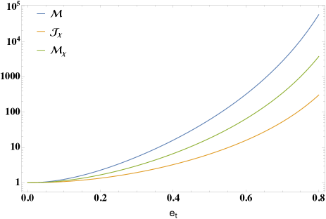
Figure 1: In this figure we plot the enhancement factors with respect to the orbital eccentricity. The figure demonstrates that the enhancement is the largest for the rate of change of mass for nonspinning black holes and is the least for the rate of change of angular momentum. However, in all the cases enhancement is significantly large depending on the eccentricity.

To estimate the impact of the eccentricity on fluxes we plot the enhancement factors in Fig. 1. In the $y-$axis enhancement factors are plotted with respect to $e_{t}$ in the $x-$axis. We find that the enhancement is the most significant for non-spinning cases. In the spinning case even though the enhancement is comparatively smaller, it can be $\mathcal{O}(10^{3})$ and $\mathcal{O}(10^{2})$ for the mass rate and angular momentum rate respectively, for high eccentricity. For circular cases, these functions take the value of the unit. However, for eccentric orbits, these factors can deviate from unit value drastically. Therefore a rate of change of mass and angular momentum can be significantly larger compared to a circular orbit. This plot explicitly demonstrates that in the leading order, the black holes lose angular momentum significantly faster when it is in an eccentric orbit. The same is also true for the mass of the black hole. The only difference is depending on the value of $\epsilon$ the black hole will either increase or decrease its mass. However, in both cases, the magnitude of the rate of change is significantly higher in an eccentric orbit. Note, in the presence of eccentricity both the flux at infinity and horizon gets enhanced. The horizon flux is a $2.5$PN effect. As a result horizon fluxes are comparatively smaller effect in comparison to leading order flux at infinity. In the eccentric case, the leading order flux at infinity gets enhanced by, $\mathcal{E}_{N}=(1+73e_{t}^{2}/24+37e_{t}^{4}/96)/(1-e_{t}^{2})^{7/2}$ Arun et al. (2009). $\mathcal{M}_{\chi}/\mathcal{E}_{N}$ can take the value $1,\,1.07033,\,3.71728,\,33.909$ respectively for $e_{t}=.1,\,.5,\,.8,\,.95$. Therefore although the horizon flux is a higher PN effect, it gets a significantly larger enhancement compared to the leading order flux at infinity in the orbital time scale. It implies that horizon fluxes are more important when $e_{t}\neq 0$.

V eccentricity evolution

In this section, we will focus on computing the eccentricity of a binary in terms of binary frequency. In this section, we will construct a prescription that can be used to find the eccentricity in terms of initial eccentricity and frequency. For a non-spinning binary, it is applicable for any PN order and arbitrarily high power of initial eccentricity. For spinning binary, it is applicable to arbitrary order of initial eccentricity and at least up to 1.5PN.

In Sec. III, we discussed that in the quasi-Keplerian approach, a parametric solution can be found considering the constants of the motions considering only the conservative part. However, during orbital motion, the system emits GWs that carry away energy and angular momentum. Due to the change in the energy and angular momentum of the orbit, the conserved quantities start to change in the inspiral time scale. This corresponds to the dissipative part of the equation of motion. Conventionally it is tackled by solving the evolution equation of the conserved quantities in the inspiral time scale. For the current work, we only require the evolution equation of the $e_{t}$ and $n$. Their evolution equation can be expressed as Arun et al. (2009); Klein and Jetzer (2010),

$$\begin{split}\left\langle\frac{dn}{dt}\right\rangle=&\frac{\eta x^{11/2}}{m^{2}(1-e_{t}^{2})^{7/2}}\left(\mathcal{N}_{n}+x\mathcal{N}_{1}+x^{3/2}\mathcal{N}_{hered}-x^{3/2}\mathcal{N}_{\beta}\right)\\ \left\langle\frac{de_{t}}{dt}\right\rangle=&\frac{-e_{t}\eta x^{4}}{m(1-e_{t}^{2})^{5/2}}\left(\mathcal{E}_{n}+x\mathcal{E}_{1}+x^{3/2}\mathcal{E}_{hered}-x^{3/2}\frac{\mathcal{E}_{\beta}}{2e_{t}^{2}}\right),\end{split}$$ (20)

where $x=\xi_{\phi}^{2/3}$. From now on in the current section, we will suppress the $\langle\rangle$ representing the average, for brevity. The above two equations can be used to find a single equation of $de_{t}/dx$. The right-hand side of the equation then can be expressed in a series expansion of $e_{t}$. The coefficients of each term will then depend on $x$. This equation then is solved to find the expression of $e_{t}$ in terms of an initial eccentricity $e_{0}$ and $\xi_{\phi}$. In this section we will develop a prescription that can be used to find very high order powers in $e_{0}$, ignoring the impact of spin in the eccentricity evolution. The impact of the spin is left for the future.

To demonstrate the prescription, we will keep up to power $e_{t}^{3}$. Then the eccentricity evolution can be expressed as follows,

$$\frac{de_{t}}{dx}= \sum_{n=1,\,{\rm odd}}^{\infty}e_{t}^{n}f_{n}(x)$$ (21)

$$\frac{de_{t}}{dx}= e_{t}f_{1}(x)+e_{t}^{3}f_{3}(x)+\mathcal{O}(e_{t}^{5})$$ (22)

Note, that we have not explicitly specified the functional expression of $f_{n}(x)$. Hence, these functions can be expanded in $x$ to arbitrarily high PN order as per the requirement. Once the prescription is described, we will substitute them with the required PN accuracy. Also note, that in the presence of spin the above equation can get modified and a different prescription may be required.

The resulting solution can be found from Eq. (21) by integrating the equation on both sides. During the process, we take $e_{t}\rightarrow e_{0}$, i.e. the initial eccentricity, when $x\rightarrow x_{0}=\xi_{\phi,0}^{2/3}$, i.e. the reference frequency. For the sake of brevity, we will demonstrate the derivation of $\mathcal{O}(e_{0}^{3})$ only. However, we will provide the result up to $\mathcal{O}(e_{0}^{5})$. We find,

$$\begin{split}\int_{e_{0}}^{e_{t}}\frac{de_{t}}{e_{t}}=&\int_{x_{0}}^{x}dx\left(f_{1}(x)+e_{t}^{2}f_{3}(x)+\mathcal{O}(e_{t}^{3})\right)\\ \ln(\frac{e_{t}}{e_{0}})=&\int_{x_{0}}^{x}dxf_{1}(x)+\int_{x_{0}}^{x}dxe_{t}^{2}f_{3}(x)+\mathcal{O}(e_{t}^{3})\\ e_{t}=&e_{0}e^{\int_{x_{0}}^{x}dxf_{1}(x)}e^{\int_{x_{0}}^{x}dxe_{t}^{2}f_{3}(x)+\mathcal{O}(e_{t}^{3})}.\end{split}$$ (23)

Note, that the first integral on the right-hand side is independent of the eccentricity while the second one is dependent. Therefore the first integral can be computed. Therefore the expression can be rearranged as,

$$e_{t}=e_{0}\frac{e^{F_{1}{(x})}}{e^{F_{1}{(x_{0})}}}e^{\int_{x_{0}}^{x}dxe_{t}^{2}f_{3}(x)+\mathcal{O}(e_{t}^{3})}.$$ (24)

The second integral has $e_{t}$ inside the integral. Therefore, without the exact knowledge of $e_{t}$ in terms of $x$ this integral can not be computed exactly. However, the eccentricity $e_{t}$ inside the second integral can be replaced with the above equation and as a result, a leading order term of the integral can be computed. Hence, although an exact integral is not computable, an approximate result can be found which is exact to a particular order. This as a result can be used to find the next order term. This can be continued for arbitrary powers of $e_{0}$. However, we will only find $e_{0}^{5}$. But in principle, this can be continued iteratively by considering higher order terms from Eq. (21). Since we have not explicitly assumed the functional form of $f_{i}(x)$, where $i$ represents the power of $e_{t}$, the individual coefficient can have higher post-Newtonian order terms included in it. Therefore, it can be used for very high PN orders. After rearranging the expressions they can be expressed as,

$$\begin{split}\frac{e_{t}e^{F_{1}{(x_{0})}}}{e_{0}e^{F_{1}{(x})}}=&e^{e_{0}^{2}\int_{x_{0}}^{x}dx\frac{e^{2F_{1}{(x})}}{e^{2F_{1}{(x_{0})}}}\left(e^{2\int_{x_{0}}^{x}d\bar{x}e_{t}^{2}f_{3}(\bar{x})+\mathcal{O}(e_{t}^{3})}\right)\,\,f_{3}(x)+\mathcal{O}(e_{t}^{3})}\\ \frac{e_{t}e^{F_{1}{(x_{0})}}}{e_{0}e^{F_{1}{(x})}}=&\left(1+e_{0}^{2}\int_{x_{0}}^{x}dx\frac{e^{2F_{1}{(x})}}{e^{2F_{1}{(x_{0})}}}\left(e^{2\int_{x_{0}}^{x}d\bar{x}e_{t}^{2}f_{3}(\bar{x})+\mathcal{O}(e_{t}^{3})}\right)\,\,f_{3}(x)+\mathcal{O}(e_{0}^{3})\right)\\ \frac{e_{t}e^{F_{1}{(x_{0})}}}{e_{0}e^{F_{1}{(x})}}=&\left(1+e_{0}^{2}\int_{x_{0}}^{x}dx\frac{e^{2F_{1}{(x})}}{e^{2F_{1}{(x_{0})}}}\left(1+\mathcal{O}(e_{0}^{2})\right)\,\,f_{3}(x)+\mathcal{O}(e_{0}^{3})\right)\end{split}$$ (25)

This as a result boils down to a series of $e_{0}$, where the coefficients of the expansions are integrals in $x$. This approach can be used consecutively after deriving individual coefficients of a particular order. Interestingly, to find the schematic structure of the coefficients in integral form of an arbitrary power of $e_{0}$ it is not required to know $f_{i}(x)$. The expression can be derived in terms of the integrals of $f_{i}(x)$s.

The above results can be expressed in a further simplified and compact form as,

$$\begin{split}e_{t}=&\frac{e^{F_{1}{(x})}}{e^{F_{1}{(x_{0})}}}(e_{0}+e_{0}^{3}\int_{x_{0}}^{x}dx\frac{e^{2F_{1}{(x})}}{e^{2F_{1}{(x_{0})}}}f_{3}(x)+\mathcal{O}(e_{0}^{4}))\end{split}$$ (26)

Continuing the similar approach even higher order expression can be found. For brevity, we demonstrate only the final result,

$$\begin{split}e_{t}=&e_{0}\frac{\mathcal{A}_{1}(x)}{\mathcal{A}_{1}(0)}+e_{0}^{3}\frac{\mathcal{A}_{1}(x)}{\mathcal{A}_{1}(0)^{3}}\left[\mathcal{A}_{3}(x)-\mathcal{A}_{3}(0)\right]+e_{0}^{5}\frac{\mathcal{A}_{1}}{\mathcal{A}_{1}(0)^{5}}[\mathcal{A}_{5}(x)-\mathcal{A}_{5}(0)+\frac{1}{2}\mathcal{A}_{3}(x)^{2}-3\mathcal{A}_{3}(x)\mathcal{A}_{3}(0)+\frac{5}{2}\mathcal{A}_{3}(0)^{2}]+\mathcal{O}(e_{0}^{7})\\ \end{split}$$ (27)

where,

$$\mathcal{A}_{1}(x)= e^{F_{1}{(x})}$$

$$\mathcal{A}_{3}(x)-\mathcal{A}_{3}(x_{0})= \int_{x_{0}}^{x}d\bar{x}e^{2F_{1}{(\bar{x}})}f_{3}(\bar{x})$$

$$\mathcal{A}_{5}(x)-\mathcal{A}_{5}(x_{0})= \int_{x_{0}}^{x}d\bar{x}\Big{(}2\mathcal{A}_{1}(\bar{x})^{2}f_{3}(\bar{x})\mathcal{A}_{3}(\bar{x})+\mathcal{A}_{1}(\bar{x})^{4}f_{5}(\bar{x})\Big{)}.$$ (28)

and $\mathcal{A}_{i}(0)=\mathcal{A}_{i}(\xi_{\phi,0})=\mathcal{A}_{i}(x_{0})$. Here we have found the expression for up to $e_{0}^{5}$. However, this approach can be continued to find the higher powers of $e_{0}$. Note, that the above equations do not depend on which PN order is considered. From higher PN calculations only the corrections to $f_{i}$s are needed. Then Eq. V can be used to find the eccentricity evolution. In B we provide the approximate expression for $\mathcal{O}(e_{0}^{7})$ and $\mathcal{O}(e_{0}^{9})$ for the nonrotating case. For the current purpose we will use $1.5$PN order expressions of $f_{1}(x)$, $f_{3}(x)$ and $f_{5}(x)$. The expressions used for $\dot{n}$ and $\dot{e}_{t}$, where overdot represents time derivative, are shown in A.

$$f_{1}(x)= -\frac{19}{12x}\left(1+\frac{(2833-5516\nu)x}{3192}+\frac{1}{456}x^{3/2}(-2452\beta_{a}-1776\beta_{b}+1131\pi)\right)$$ (29)

$$f_{3}(x)= \frac{3323}{576x}\left(1+\frac{(472943-653228\nu)x}{159504}+\frac{x^{3/2}(-353345\beta_{a}-270423\beta_{b}+159321\pi)}{39876}\right)$$ (30)

$$f_{5}(x)= -\frac{225431}{13824x}\left(1+\frac{(232485915-285412372\nu)x}{37872408}+x^{3/2}\left(\frac{-6313343\beta_{a}-4954393\beta_{b}}{450862}+\frac{11212300784165054871261\pi}{1761179687500000000000}\right)\right).$$ (31)

Then further computation can be done using Eq. (V). In the following, we show the expressions up to $1.5$PN in terms of $\xi_{\phi}$,

$$\mathcal{A}_{1}(\xi_{\phi})=\xi_{\phi}^{-19/18}(1+\frac{(5516\nu-2833)\xi_{\phi}^{2/3}}{2016}+\frac{1}{432}\xi_{\phi}(2452\beta_{a}+1776\beta_{b}-1131\pi))$$ (32)

$$\begin{split}\mathcal{A}_{3}(\xi_{\phi})=-\frac{3323}{1824\xi_{\phi}^{19/9}}\left(1+\frac{19(576485\nu+64718)\xi_{\phi}^{2/3}}{5443074}-\frac{19\xi_{\phi}(890535\pi-2(893893\beta_{a}+517017\beta_{b}))}{7177680}\right)\end{split}$$ (33)

$$\begin{split}\mathcal{A}_{5}(\xi_{\phi})=&\frac{19608707}{3326976\xi_{\phi}^{38/9}}\Bigg{(}1+\frac{95(21825056708\nu+2829020183)\xi_{\phi}^{2/3}}{513904993056}\\ &+\frac{19\xi_{\phi}}{58826121}\left(\frac{59}{5220}(2824399609\beta_{a}+1699967901\beta_{b})-\frac{2633309468007384992014369\pi}{169921875000000000}\right)\Bigg{)}\end{split}$$ (34)

$$\begin{split}\mathcal{A}_{1}(\xi_{\phi})\mathcal{A}_{3}(\xi_{\phi})=&-\frac{3323}{1824\xi_{\phi}^{19/6}}\left(1+\frac{(137845708\nu-34236165)\xi_{\phi}^{2/3}}{29029728}+\frac{\xi_{\phi}(12451319\beta_{a}+8192481\beta_{b}-5951955\pi)}{1196280}\right)\end{split}$$ (35)

$$\begin{split}\mathcal{A}_{1}(\xi_{\phi})\mathcal{A}_{5}(\xi_{\phi})=&\frac{19608707}{3326976\xi_{\phi}^{95/18}}\Bigg{(}1+\frac{(248534396344\nu-32386582337)\xi_{\phi}^{2/3}}{36707499504}\\ &+\frac{-228607670547148483607319033\pi\xi_{\phi}}{29987534337890625000000000}+\frac{\xi_{\phi}(47940155111171875000\beta_{a}+30938208727353515625\beta_{b})}{2998753433789062500}\Bigg{)}\end{split}$$ (36)

$$\begin{split}\mathcal{A}_{1}(\xi_{\phi})\mathcal{A}_{3}(\xi_{\phi})^{2}=\frac{11042329}{3326976\xi_{\phi}^{95/18}}\left(1+\frac{(588788564\nu-83034223)\xi_{\phi}^{2/3}}{87089184}+\frac{\xi_{\phi}(108675848\beta_{a}+68801532\beta_{b}-52631895\pi)}{7177680}\right)\end{split}$$ (37)

These newly found results are consistent with the leading order result found in Ref. Yunes et al. (2009). These expressions will be used in the next section to compute the horizon fluxes in series of $e_{0}$ and $\xi_{\phi}$. In an inspiral, as discussed above, the orbital elemnts such as eccentricity and latus rectum are not fixed quantity. With the loss of GWs these quantities evolve. With the inspiral the frequency of the emitted GW also evolves. Therefore, modelling the waveforms in frequency domain requires the evolution equations of the orbital quantities. Finding the fluxes and orbital quantities in terms of $e_{t}$ and $\xi_{\phi}$, is not sufficient to construct a frequency domain waveform in the manner of Moore et al. (2016). However, once the $e_{t}$ is expressed in terms of an initial eccentricity and GW frequency $\sim\xi_{\phi}$, stationary phase approximation can be used to find the phase and amplitude of the emitted GW in the frequency domain Tichy et al. (2000). For that purpose, expressing the fluxes in terms of $\xi_{\phi}$ and “unchanging quantities”, such as $e_{0}$, will help in constructing frequency domain waveforms.

VI Rate of change of mass and angular momentum from L.O. term

In section IV, we found the average leading order fluxes for both the spinning and non-spinning BHs. We showed that eccentricity makes the TH much stronger compared to a circular orbit. However, the expressions were computed in terms of $e_{t}$ which changes over time due to the GW emission. Expressing the results in terms of $\xi$ is also not useful as it is not directly connected to the frequency of the emitted GW, unlike $\xi_{\phi}$. Using the results derived in the previous sections here we will re-express them in terms of the initial eccentricity $e_{0}$ and $\xi_{\phi}$.

The effect of the eccentricity arising only via the enhancement factors and $\xi$. Therefore we only need to do series expansion of $\xi^{6}\mathcal{M}$, $\xi^{4}\mathcal{J}_{\chi}$ and $\xi^{5}\mathcal{M}_{\chi}$. After using the dependence of $\xi$ and the enhancement factors on $e_{0}$ and $\xi_{\phi}$ we find,

$$\begin{split}\langle\dot{m}_{1}\rangle=&\frac{32m_{1}^{6}m_{2}^{2}\xi_{\phi}^{6}}{5M^{8}}\left(\mathcal{M}_{0}+e_{0}^{2}\mathcal{M}_{2}+e_{0}^{4}\mathcal{M}_{4}+e_{0}^{6}\mathcal{M}_{6}\right)\\ \langle\dot{m}_{1}\rangle_{\chi\neq 0}=&-\frac{8\epsilon m_{1}^{5}m_{2}^{2}\chi\left(3\chi^{2}+1\right)}{5M^{7}}\xi_{\phi}^{5}\left(\mathcal{M}_{\chi 0}+e_{0}^{2}\mathcal{M}_{\chi 2}+e_{0}^{4}\mathcal{M}_{\chi 4}+e_{0}^{6}\mathcal{M}_{\chi 6}\right)\\ \langle\dot{J}_{1}\rangle=&-\frac{8m_{1}^{5}m_{2}^{2}\chi\left(3\chi^{2}+1\right)\xi_{\phi}^{4}}{5M^{6}}\left(\mathcal{J}_{0}+e_{0}^{2}\mathcal{J}_{2}+e_{0}^{4}\mathcal{J}_{4}+e_{0}^{6}\mathcal{J}_{6}\right)\end{split}$$ (38)

The coefficents $\mathcal{M}_{i}$, $\mathcal{M}_{\chi i}$, and $\mathcal{J}_{i}$ can be expressed in postNewtonian expansion. Hence, each of these coefficients is a series expansion in $\xi_{\phi}$. We find,

$$\begin{split}\mathcal{M}_{0}=&1-18\xi_{\phi}^{2/3}\\ \mathcal{M}_{\chi 0}=&1-15\xi_{\phi}^{2/3}\\ \mathcal{J}_{0}=&1-12\xi_{\phi}^{2/3}\end{split}$$ (39)

$$\begin{split}\mathcal{M}_{2}=&\frac{23}{A(0)^{2}\xi_{\phi}^{19/9}}\left(1+\left(\frac{197\eta}{36}-\frac{500615}{23184}\right)\xi_{\phi}^{2/3}-\frac{377\pi\xi_{\phi}}{72}\right)\\ \mathcal{M}_{\chi 2}=&\frac{27}{2A(0)^{2}\xi_{\phi}^{19/9}}\left(1+\left(\frac{197\eta}{36}-\frac{19073}{1008}\right)\xi_{\phi}^{2/3}+\left(\frac{613\beta_{a}}{54}+\frac{74\beta_{b}}{9}-\frac{377\pi}{72}\right)\xi_{\phi}\right)\\ \mathcal{J}_{2}=&\frac{15}{2A(0)^{2}\xi_{\phi}^{19/9}}\left(1+\left(\frac{197\eta}{36}-\frac{82709}{5040}\right)\xi_{\phi}^{2/3}+\left(\frac{613\beta_{a}}{54}+\frac{74\beta_{b}}{9}-\frac{377\pi}{72}\right)\xi_{\phi}\right)\end{split}$$ (40)

$$\mathcal{M}_{4}=\frac{87731}{912\mathcal{A}_{1}(0)^{4}\xi_{\phi}^{38/9}}\left(1+\frac{(16047208268\nu-34575397879)\xi_{\phi}^{2/3}}{1149627024}-\frac{2459723415\pi}{189498960}\xi_{\phi}\right)$$ (41)

$$\mathcal{M}_{\chi 4}=\frac{13641}{608\mathcal{A}_{1}(0)^{4}\xi_{\phi}^{38/9}}\left(1+\frac{(157727492\nu-293973805)\xi_{\phi}^{2/3}}{8511984}+\frac{\xi_{\phi}(365520958\beta_{a}+279618942\beta_{b}-164842035\pi)}{9821520}\right)$$ (42)

$$\mathcal{J}_{4}=-\frac{655}{608\mathcal{A}_{1}(0)^{4}\xi_{\phi}^{38/9}}\left(1+\frac{(974157013-659362340\nu)\xi_{\phi}^{2/3}}{8583120}+\frac{\xi_{\phi}(-41087786\beta_{a}-34716714\beta_{b}+17699745\pi)}{282960}\right)$$ (43)

$$\begin{split}\mathcal{M}_{6}=&-\frac{5862821}{138624\mathcal{A}_{1}(0)^{6}\xi_{\phi}^{19/3}}\Bigg{(}1+\frac{(5462576860497-4428488210692\nu)\xi_{\phi}^{2/3}}{204870417024}+\frac{70720269710659580653919917\pi}{3984886148437500000000000}\xi_{\phi}\Bigg{)}\end{split}$$ (44)

$$\begin{split}\mathcal{M}_{\chi 6}=&-\frac{2369655}{92416\mathcal{A}_{1}(0)^{6}\xi_{\phi}^{19/3}}\Bigg{(}1+\frac{17(9084331932\nu-15050525335)\xi_{\phi}^{2/3}}{11829317760}\\ &+\xi_{\phi}\left(\frac{185481144929\beta_{a}+122831019561\beta_{b}}{8246399400}-\frac{5990691756574973175575663\pi}{536874960937500000000000}\right)\Bigg{)}\end{split}$$ (45)

$$\begin{split}\mathcal{J}_{6}=&\frac{1157705}{92416\mathcal{A}_{1}(0)^{6}\xi_{\phi}^{19/3}}\Bigg{(}1+\frac{(73579104553-56767003748\nu)\xi_{\phi}^{2/3}}{8090968704}\\ &+\xi_{\phi}\left(\frac{-11940702143\beta_{a}-17960217927\beta_{b}}{2417288040}+\frac{282538595290616058525221\pi}{157375523437500000000000}\right)\Bigg{)}\end{split}$$ (46)

These expressions of rates of change of mass and angular momentum of the black hole induce an exchange of energy and angular momentum between the orbit and the black hole due to the conservation of total energy and angular momentum. Therefore these are nothing but the fluxes of orbital energy and orbital angular momentum, namely $-\frac{dE}{dt}$ and $-\frac{dL}{dt}$. This rate of change of orbital conserved quantities, therefore, backreacts on the orbit affecting the inspiral rate of binary and as a result the emitted GW. Note, sub-leading terms in $\xi_{\phi}$ are incomplete as only the leading order term of $\xi$ has been considered. In future work we will compute the subleading terms in $\xi$ which will lead to completion of the subleading terms in $\xi_{\phi}$.

VII Discussion and conclusion

In this paper, we explored the tidal heating of black holes in an eccentric orbit. We only focused on the leading order effect of $\xi$. However, it is of necessary importance to explore the next-order effects. However, currently, there are discrepant results in the literature regarding the next-to-next-leading order results in circular orbits Saketh et al. (2023). In Ref. Saketh et al. (2023) they found that the result does not match with Chatziioannou et al. (2016) in the generic mass ratio case. However in the test mass limit, their result matches with Ref. Tagoshi et al. (1997). Therefore, this can lead to similar discrepancies in eccentric cases too. This is the reason why we focused only on the leading order result. It is very important to look into the details of the discrepancies and come up with a possible resolution. We will look into this aspect in the future while investigating the next-to-leading order and next-to-next leading order effect in an eccentric orbit. This aspect needs to be studied in detail as the next-generation detectors and space-based detectors will be sensitive to small deviations. Inadequate modeling therefore can lead to a wrong inference of the parameters. Secondly, sources like extreme mass ratio inspirals are expected to have large eccentricities. These sources also demonstrate strong tidal heating effects in the observable band. Therefore, it is crucial that the horizon fluxes are modeled appropriately so that the waveform models reach the required accuracy during observation.

In the process, we also explored the eccentricity evolution of a binary. We developed a prescription that can be used iteratively to find very high-order terms in both the post-Newtonian variable as well as the initial eccentricity $e_{0}$. We provided the general expression for the coefficient of $\mathcal{O}(e_{0}^{n})$, for up to $n=5$. This expression is valid arbitrary higher PN correction in the functions $f_{i}(x)$ as long as Eq. 21 stays unchanged. With more updated expressions for $f_{i}(x)$ the correction in the eccentricity evolution can be computed in a straightforward manner using the expression provided here in Eq. 27. In the appendix, we also provide an approximate expression for $\mathcal{O}(e_{0}^{n})$ for arbitrary $n$ and use it to compute the expression for $n=7,9$ in the non-spinning limit.

In the current work, we found that the eccentricity effects are very strong. The horizon fluxes can change significantly from circular orbit results. This is primarily due to the enhancement factor. Depending on the value of the eccentricity, the enhancement factors for horizon energy flux can be as large as $10^{4}$ for non-spinning bodies and $10^{3}$ for spinning bodies. This as a result creates a correlation between the eccentricity of the orbits and the spins of the body. This may lead to a better understanding of the properties of the population distributions of observed black holes. These aspects need much more detailed analysis from both the theory and observational sides.

Appendix A Expressions for rates

In this section we will explicitly demonstrate the expression for rate of change of eccentricity. The required expressions are as follows Arun et al. (2009); Klein and Jetzer (2010):

$$\mathcal{N}_{n}= \frac{1}{5}(96+292e_{t}^{2}+37e_{t}^{4})$$ (47)

$$\mathcal{N}_{1}= \frac{1}{(1-e_{t}^{2})}(-\frac{4846}{35}-\frac{264\nu}{5}+e_{t}^{2}(\frac{5001}{35}-570\nu)+e_{t}^{4}(\frac{2489}{4}-\frac{5061\nu}{10})+e_{t}^{6}(\frac{11717}{280}-\frac{148\nu}{5})$$ (48)

$$\mathcal{N}_{hered}= 4\pi\frac{96(1-e_{t}^{2})^{7/2}}{5}\varphi(e_{t})$$ (49)

$$\mathcal{N}_{\beta}= \frac{1}{10(1-e_{t}^{2})^{3/2}}\beta(3088+15528e_{t}^{2}+7026e_{t}^{4}+195e_{t}^{6},2160+11720e_{t}^{2}+5982e_{t}^{4}+207e_{t}^{6}).$$ (50)

$$\mathcal{E}_{n}= (\frac{304}{15}+\frac{121}{15}e_{t}^{2})$$ (51)

$$\mathcal{E}_{1}= \frac{1}{(1-e_{t}^{2})}(-\frac{939}{35}-\frac{4084\nu}{45}+e_{t}^{2}(\frac{29917}{105}-\frac{7753}{30}\nu)+e_{t}^{4}(\frac{13929}{280}-\frac{1664\nu}{45})$$ (52)

$$\mathcal{E}_{hered}= \frac{32}{5}\frac{985(1-e_{t}^{2})^{5/2}}{48}\pi\varphi_{e}(e_{t})$$ (53)

$$\mathcal{E}_{\beta}= \frac{e_{t}^{2}}{15(1-e_{t}^{2})^{3/2}}\beta(13048+12000e_{t}^{2}+789e_{t}^{4},9208+10026e_{t}^{2}+835e_{t}^{4}).$$ (54)

Expression for $\varphi(e_{t})$ is taken from Forseth et al. (2016). Expression of $\varphi_{e}(e_{t})$ is provided in Arun et al. (2009) in terms of different functions, from which up to $\mathcal{O}(e_{t}^{4})$ can be computed. The other terms are computed from higher order terms of $\tilde{\varphi}(e_{t})$ in Tanay et al. (2016).

$$\varphi(e_{t})= \frac{1}{(1-e_{t}^{2})^{5}}(1+\frac{1375}{192}e_{t}^{2}+\frac{3935}{768}e_{t}^{4}+\frac{10007}{36864}e_{t}^{6}+\frac{2321}{884736}e_{t}^{8}+\frac{237857}{353894400}e_{t}^{10})$$ (55)

$$\varphi_{e}(e_{t})= \frac{192}{985}\frac{\sqrt{1-e_{t}^{2}}}{e_{t}^{2}}\left(\sqrt{1-e_{t}^{2}}\varphi(e_{t})-\tilde{\varphi}(e_{t})\right)$$ (56)

$$\tilde{\varphi}(e_{t})= 1+\frac{209}{32}e_{t}^{2}+\frac{2415}{128}e_{t}^{4}+\frac{317166232530923893657}{8000000000000000000}e_{t}^{6}+\frac{280916856316939384413751040219}{4000000000000000000000000000}e_{t}^{8},$$ (57)

$$\beta(a,b)= a\beta_{a}+b\beta_{b}$$ (58)

$$\beta_{a}= {\bf\hat{J}.{\bf\zeta}}$$ (59)

$$\beta_{b}= {\bf\hat{J}.{\bf\xi}}$$ (60)

$${\bf\zeta}= {\bf S_{1}}+{\bf S_{2}}$$ (61)

$${\bf\xi}= \frac{m_{2}}{m_{1}}{\bf S_{1}}+\frac{m_{1}}{m_{2}}{\bf S_{2}},$$ (62)

where ${\bf S}_{i}$ are the individual spins and ${\bf J}$ is the reduced orbital angular momentum discussed in Ref. Klein and Jetzer (2010). ${\bf J}$ helps encapsulate the effects of spin precession. It can be checked from Eq. (10) in Ref. Klein and Jetzer (2010), when the spins of the bodies are either aligned or antialigned with the direction perpendicular to the orbital plane, say $\hat{\bf L}$, ${\bf J}$ is also aligned or antialigned with $\hat{\bf L}$. In such a case therefore, $\hat{\bf J}||\hat{\bf L}$. Using the above expressions it is straightforward to compute $f_{i}(\xi_{\phi})$s.

Appendix B Higher order terms of $e_{0}$

From the formalism, it is straightforward to check that the term in the expression of $e_{t}$ corresponding to $e_{0}^{n}$ will consist of a term,

$$\mathcal{O}(e_{0}^{n})=\frac{\mathcal{A}_{1}(x)}{\mathcal{A}_{1}(0)}e_{0}^{n}\int_{x_{0}}^{x}\frac{\mathcal{A}_{1}(\bar{x})^{n-1}}{\mathcal{A}_{1}(0)^{n-1}}f_{n-1}(\bar{x})d\bar{x}+{\rm other\,\,terms}.$$ (63)

Although it is time-consuming to find the complete expression for $\mathcal{O}(e_{0}^{n})$, it is easier to evaluate the above integral to find an approximate result. For exactness rest of the terms must be found in the manner discussed previously. In this way, we will find the approximate result for several higher-order terms below in the nonspinning limit.

$$f_{7}(x)=\frac{15718757}{331776x}\left(1+\frac{(49486716031-57934888172\nu)x}{5281502352}+\frac{66835188610235794715208146757739\pi x^{3/2}}{7675174316406250000000000000000}\right)$$ (64)

$$f_{9}(x)=-\frac{1097423579}{7962624x}\left(1+\frac{(1161963898391-1327655382368\nu)x}{92183580636}+\frac{370344540064784477905382804708442045113261\pi x^{3/2}}{33490709808349609375000000000000000000000}\right)$$ (65)

$$\mathcal{O}(e_{0}^{7})\sim\frac{\mathcal{A}_{1}(x)}{\mathcal{A}_{1}(0)}e_{0}^{7}\int_{x_{0}}^{x}\frac{\mathcal{A}_{1}(\bar{x})^{6}}{\mathcal{A}_{1}(0)^{6}}f_{7}(\bar{x})d\bar{x}=\frac{\mathcal{A}_{1}(x)e_{0}^{7}}{\mathcal{A}_{1}(0)^{7}}\left[\mathcal{A}_{7}(x)-\mathcal{A}_{7}(0)\right]$$ (66)

$$\mathcal{O}(e_{0}^{9})\sim\frac{\mathcal{A}_{1}(x)}{\mathcal{A}_{1}(0)}e_{0}^{9}\int_{x_{0}}^{x}\frac{\mathcal{A}_{1}(\bar{x})^{8}}{\mathcal{A}_{1}(0)^{8}}f_{9}(\bar{x})d\bar{x}=\frac{\mathcal{A}_{1}(x)e_{0}^{9}}{\mathcal{A}_{1}(0)^{9}}\left[\mathcal{A}_{9}(x)-\mathcal{A}_{9}(0)\right]$$ (67)

$$\mathcal{A}_{7}(\xi_{\phi})=-\frac{827303}{165888\xi_{\phi}^{19/3}}\left(1+\frac{5(410996792\nu+70792535)\xi_{\phi}^{2/3}}{337539624}-\frac{161187023829937147104375559726783\pi\xi_{\phi}}{19389914062500000000000000000000}\right)$$ (68)

$$\begin{split}\mathcal{A}_{9}(\xi_{\phi})=\frac{1097423579}{100859904\xi_{\phi}^{76/9}}\Bigg{(}1&+\frac{19(1035211157330\nu+188445347933)\xi_{\phi}^{2/3}}{2419818991695}\\ &-\frac{56618060827525980254742040394856410285632369\pi\xi_{\phi}}{5048724503608703613281250000000000000000000}\Bigg{)}\end{split}$$ (69)

$$\mathcal{A}_{1}(\xi_{\phi})\mathcal{A}_{7}(\xi_{\phi})=-\frac{827303}{165888\xi_{\phi}^{133/18}}\left(1+\frac{(250196509556\nu-10110875083)\xi_{\phi}^{2/3}}{28353328416}-\frac{635852688189030191313126679180349\pi\xi_{\phi}}{58169742187500000000000000000000}\right)$$ (70)

$$\begin{split}\mathcal{A}_{1}(\xi_{\phi})\mathcal{A}_{9}(\xi_{\phi})=\frac{1097423579}{100859904\xi_{\phi}^{57/6}}\Bigg{(}1&+\frac{(280425659939460\nu+1919912189173)\xi_{\phi}^{2/3}}{25811402578080}\\ &-\frac{7759544673629801249143429835539601142848041\pi\xi_{\phi}}{560969389289855957031250000000000000000000}\Bigg{)}\end{split}$$ (71)

References

- Aasi et al. (2015) J. Aasi et al. (LIGO Scientific), Class. Quant. Grav. 32, 074001 (2015), eprint 1411.4547.
- Acernese et al. (2015) F. Acernese et al. (VIRGO), Class. Quant. Grav. 32, 024001 (2015), eprint 1408.3978.
- Abbott et al. (2019a) B. P. Abbott et al. (LIGO Scientific, Virgo), Phys. Rev. X9, 031040 (2019a), eprint 1811.12907.
- Abbott et al. (2021a) R. Abbott et al. (LIGO Scientific, Virgo), Phys. Rev. X 11, 021053 (2021a), eprint 2010.14527.
- Abbott et al. (2019b) B. P. Abbott et al. (LIGO Scientific, Virgo), Phys. Rev. D100, 104036 (2019b), eprint 1903.04467.
- Abbott et al. (2019c) B. P. Abbott et al. (LIGO Scientific, Virgo), Phys. Rev. Lett. 123, 011102 (2019c), eprint 1811.00364.
- Cardoso et al. (2017) V. Cardoso, E. Franzin, A. Maselli, P. Pani, and G. Raposo, Phys. Rev. D 95, 084014 (2017), [Addendum: Phys.Rev.D 95, 089901 (2017)], eprint 1701.01116.
- Abbott et al. (2017) B. P. Abbott et al. (Virgo, LIGO Scientific), Phys. Rev. Lett. 119, 161101 (2017), eprint 1710.05832.
- Abbott et al. (2020) B. Abbott et al. (LIGO Scientific, Virgo), Astrophys. J. Lett. 892, L3 (2020), eprint 2001.01761.
- Abbott et al. (2021b) R. Abbott et al. (LIGO Scientific, KAGRA, VIRGO), Astrophys. J. Lett. 915, L5 (2021b), eprint 2106.15163.
- Maggiore et al. (2020) M. Maggiore, C. Van Den Broeck, N. Bartolo, E. Belgacem, D. Bertacca, M. A. Bizouard, M. Branchesi, S. Clesse, S. Foffa, J. García-Bellido, et al., Journal of Cosmology and Astroparticle Physics 2020, 050 (2020).
- Reitze et al. (2019) D. Reitze et al., Bull. Am. Astron. Soc. 51, 035 (2019), eprint 1907.04833.
- Amaro-Seoane et al. (2017) P. Amaro-Seoane et al. (LISA) (2017), eprint 1702.00786.
- Thorne et al. (1986) K. S. Thorne, R. Price, and D. Macdonald, Black holes: the membrane paradigm (Yale University Press, 1986).
- Damour (1982) T. Damour, in Pulsating relativistic stars (1982).
- Poisson (2009) E. Poisson, Phys. Rev. D80, 064029 (2009), eprint 0907.0874.
- Cardoso and Pani (2013) V. Cardoso and P. Pani, Class. Quant. Grav. 30, 045011 (2013), eprint 1205.3184.
- Hartle (1973) J. B. Hartle, Phys. Rev. D8, 1010 (1973).
- Hughes (2001) S. A. Hughes, Phys. Rev. D64, 064004 (2001), [Erratum: Phys. Rev.D88,no.10,109902(2013)], eprint gr-qc/0104041.
- Poisson and Will (1953) E. Poisson and C. Will, Gravity: Newtonian, Post-Newtonian, Relativistic (Cambridge University Press, Cambridge, UK, 1953).
- Maselli et al. (2018) A. Maselli, P. Pani, V. Cardoso, T. Abdelsalhin, L. Gualtieri, and V. Ferrari, Phys. Rev. Lett. 120, 081101 (2018), eprint 1703.10612.
- Datta and Bose (2019) S. Datta and S. Bose, Phys. Rev. D99, 084001 (2019), eprint 1902.01723.
- Datta et al. (2020) S. Datta, R. Brito, S. Bose, P. Pani, and S. A. Hughes, Phys. Rev. D101, 044004 (2020), eprint 1910.07841.
- Datta (2020) S. Datta, Phys. Rev. D 102, 064040 (2020), eprint 2002.04480.
- Agullo et al. (2021) I. Agullo, V. Cardoso, A. D. Rio, M. Maggiore, and J. Pullin, Phys. Rev. Lett. 126, 041302 (2021), eprint 2007.13761.
- Chakraborty et al. (2021) S. Chakraborty, S. Datta, and S. Sau, Phys. Rev. D 104, 104001 (2021), eprint 2103.12430.
- Sherf (2021) Y. Sherf, Phys. Rev. D 103, 104003 (2021), eprint 2104.03766.
- Datta and Phukon (2021) S. Datta and K. S. Phukon, Phys. Rev. D 104, 124062 (2021), eprint 2105.11140.
- Sago and Tanaka (2021) N. Sago and T. Tanaka, Phys. Rev. D 104, 064009 (2021), eprint 2106.07123.
- Maggio et al. (2021) E. Maggio, M. van de Meent, and P. Pani, Phys. Rev. D 104, 104026 (2021), eprint 2106.07195.
- Sago and Tanaka (2022) N. Sago and T. Tanaka (2022), eprint 2202.04249.
- Pretorius (2007) F. Pretorius (2007), eprint 0710.1338.
- Sasaki and Tagoshi (2003) M. Sasaki and H. Tagoshi, Living Rev. Rel. 6, 6 (2003), eprint gr-qc/0306120.
- Datta et al. (2021) S. Datta, K. S. Phukon, and S. Bose, Phys. Rev. D 104, 084006 (2021), eprint 2004.05974.
- Mukherjee et al. (2022) S. Mukherjee, S. Datta, S. Tiwari, K. S. Phukon, and S. Bose, Phys. Rev. D 106, 104032 (2022), eprint 2202.08661.
- Taylor and Poisson (2008) S. Taylor and E. Poisson, Phys. Rev. D 78, 084016 (2008), eprint 0806.3052.
- Damour and Schaefer (1988) T. Damour and G. Schaefer, Nuovo Cim. B 101, 127 (1988).
- Schäfer and Wex (1993) G. Schäfer and N. Wex, , Phys. Lett. A 174, 196 (1993).
- Moore et al. (2016) B. Moore, M. Favata, K. G. Arun, and C. K. Mishra, Phys. Rev. D 93, 124061 (2016), eprint 1605.00304.
- Memmesheimer et al. (2004) R.-M. Memmesheimer, A. Gopakumar, and G. Schaefer, Phys. Rev. D 70, 104011 (2004), eprint gr-qc/0407049.
- Konigsdorffer and Gopakumar (2006) C. Konigsdorffer and A. Gopakumar, Phys. Rev. D 73, 124012 (2006), eprint gr-qc/0603056.
- Damour et al. (2004) T. Damour, A. Gopakumar, and B. R. Iyer, Phys. Rev. D 70, 064028 (2004), eprint gr-qc/0404128.
- Peters and Mathews (1963) P. C. Peters and J. Mathews, Phys. Rev. 131, 435 (1963).
- Alvi (2001) K. Alvi, Phys. Rev. D64, 104020 (2001), eprint gr-qc/0107080.
- Forseth (2016) E. R. Forseth, Ph.D. thesis (2016), URL https://www.proquest.com/dissertations-theses/high-precision-extreme-mass-ratio-inspirals-black/docview/1805911512/se-2.
- Poisson (2004) E. Poisson, Phys. Rev. D70, 084044 (2004), eprint gr-qc/0407050.
- Saketh et al. (2023) M. V. S. Saketh, J. Steinhoff, J. Vines, and A. Buonanno, Phys. Rev. D 107, 084006 (2023), eprint 2212.13095.
- Chatziioannou et al. (2013) K. Chatziioannou, E. Poisson, and N. Yunes, Phys. Rev. D87, 044022 (2013), eprint 1211.1686.
- Chatziioannou et al. (2016) K. Chatziioannou, E. Poisson, and N. Yunes, Phys. Rev. D94, 084043 (2016), eprint 1608.02899.
- Isoyama et al. (2022) S. Isoyama, R. Fujita, A. J. K. Chua, H. Nakano, A. Pound, and N. Sago, Phys. Rev. Lett. 128, 231101 (2022), eprint 2111.05288.
- Arun et al. (2009) K. G. Arun, L. Blanchet, B. R. Iyer, and S. Sinha, Phys. Rev. D 80, 124018 (2009), eprint 0908.3854.
- Klein and Jetzer (2010) A. Klein and P. Jetzer, Phys. Rev. D 81, 124001 (2010), eprint 1005.2046.
- Yunes et al. (2009) N. Yunes, K. G. Arun, E. Berti, and C. M. Will, Phys. Rev. D 80, 084001 (2009), [Erratum: Phys.Rev.D 89, 109901 (2014)], eprint 0906.0313.
- Tichy et al. (2000) W. Tichy, E. E. Flanagan, and E. Poisson, Phys. Rev. D61, 104015 (2000), eprint gr-qc/9912075.
- Tagoshi et al. (1997) H. Tagoshi, S. Mano, and E. Takasugi, Prog. Theor. Phys. 98, 829 (1997), eprint gr-qc/9711072.
- Forseth et al. (2016) E. Forseth, C. R. Evans, and S. Hopper, Phys. Rev. D 93, 064058 (2016), eprint 1512.03051.
- Tanay et al. (2016) S. Tanay, M. Haney, and A. Gopakumar, Phys. Rev. D 93, 064031 (2016), eprint 1602.03081.