Electroweak input schemes and universal corrections in SMEFT

Abstract

The choice of an electroweak (EW) input scheme is an important component of perturbative calculations in Standard Model Effective Field Theory (SMEFT). In this paper we perform a systematic study of three different EW input schemes in SMEFT, in particular those using the parameter sets $\{M_{W},\,M_{Z},\,G_{F}\}$, $\{M_{W},\,M_{Z},\,\alpha\}$, or $\{\alpha,\,M_{Z},\,G_{F}\}$. We discuss general features and calculate decay rates of $Z$ and $W$ bosons to leptons and Higgs decays to bottom quarks in these three schemes up to next-to-leading order (NLO) in dimension-six SMEFT. We explore the sensitivity to Wilson coefficients and perturbative convergence in the different schemes, and show that while the latter point is more involved than in the Standard Model, the dominant scheme-dependent NLO corrections are universal and can be taken into account by a simple set of substitutions on the leading-order results. Residual NLO corrections are then of similar size between the different input schemes, and performing calculations in multiple schemes can give a useful handle on theory uncertainties in SMEFT predictions and fits to data.

1 Introduction

Standard Model Effective Field Theory (SMEFT) is an important tool for investigating small deviations from Standard Model (SM) predictions. Such indirect descriptions of new physics can be made more robust by including quantum corrections not only in the SM, but also in SMEFT. Indeed, the study of next-to-leading order (NLO) corrections (and in a few instances next-to-next-to-leading order (NNLO) corrections) in dimension-six SMEFT has received much attention in recent years, either calculated on a case-by-case basis for specific processes, Zhang:2013xya ; Crivellin:2013hpa ; Zhang:2014rja ; Pruna:2014asa ; Grober:2015cwa ; Hartmann:2015oia ; Ghezzi:2015vva ; Hartmann:2015aia ; Zhang:2016omx ; BessidskaiaBylund:2016jvp ; Maltoni:2016yxb ; Degrande:2016dqg ; Hartmann:2016pil ; Grazzini:2016paz ; deFlorian:2017qfk ; Deutschmann:2017qum ; Baglio:2017bfe ; Dawson:2018pyl ; Degrande:2018fog ; Vryonidou:2018eyv ; Dedes:2018seb ; Grazzini:2018eyk ; Dawson:2018liq ; Dawson:2018jlg ; Dawson:2018dxp ; Neumann:2019kvk ; Dedes:2019bew ; Boughezal:2019xpp ; Dawson:2019clf ; Baglio:2019uty ; Haisch:2020ahr ; David:2020pzt ; Dittmaier:2021fls ; Dawson:2021ofa ; Boughezal:2021tih ; Battaglia:2021nys ; Kley:2021yhn ; Faham:2021zet ; Haisch:2022nwz ; Heinrich:2022idm ; Bhardwaj:2022qtk ; Asteriadis:2022ras ; Bellafronte:2023amz or moving towards full automation as in the case of QCD corrections Degrande:2020evl .

An important consideration for SMEFT predictions and fits is the choice of the electroweak (EW) input scheme. Ideally, the input parameters should be measured with very high accuracy such that their effect on SMEFT fits is subdominant or even negligible. However, even beyond that, the choice of the input parameters influences perturbative convergence as well as the pattern of Wilson coefficients appearing in leading-order (LO) and NLO predictions. Typical choices of the input parameters include the Fermi constant $G_{F}$, the mass of the $W$ and $Z$ bosons, $M_{W}$ and $M_{Z}$, as well as the electromagnetic coupling constant $\alpha$. Invariably, the NLO SMEFT calculations described above have been performed in one of three different schemes, which use either $\{M_{W},\,M_{Z},\,G_{F}\}$ ($\alpha_{\mu}$ scheme), $\{M_{W},\,M_{Z},\,\alpha\}$ ($\alpha$ scheme) or $\{\alpha,\,M_{Z},\,G_{F}\}$ (LEP scheme) as inputs. Some discussions of these input schemes can be found in Brivio:2017bnu ; Brivio:2021yjb . However, there has been no systematic study which elucidates general features of these EW input schemes beyond LO in SMEFT, much less a numerical exploration of benchmark results at NLO in the different schemes. The aim of this paper is to fill this gap.

We structure the discussion as follows. First, in Section 2, we describe the ingredients needed to construct UV renormalised amplitudes in the three schemes, introducing a notation that makes the connections between them transparent. In Section 3 we identify salient features of the different schemes, including patterns of perturbative convergence and Wilson coefficients associated with finite parts of counterterms for typical weak or electromagnetic vertices. We give a first set of NLO results at the level of derived parameters such as $M_{W}$ in the LEP scheme or $G_{F}$ in the $\alpha$ scheme in Section 4, also laying out our method for estimating perturbative uncertainties from scale variations in the SM and SMEFT. In Section 5 we perform a thorough numerical analysis of heavy boson decays at NLO in SMEFT in the three schemes, covering $W$ and $Z$ decay into leptons, and Higgs decay into bottom quarks. Finally, drawing on the insights from the aforementioned sections, we propose in Section 6 a simple procedure which can be used to deduce a set of universal and numerically dominant input-scheme dependent NLO corrections in SMEFT. Concluding remarks are given in Section 7.

While the main focus of the paper is to elucidate the role of EW input schemes in SMEFT, as a by-product we have produced quite a few NLO results which were not available in the literature so far. These have been obtained using an in-house FeynRules Alloul:2013bka implementation of the dimension-six SMEFT Lagrangian, and cross checked with SMEFTsim Brivio:2017btx ; Brivio:2020onw . Matrix elements were computed using FeynArts and FormCalc Hahn:2016ebn ; Hahn:1998yk ; Hahn:2000kx , analytic results for Feynman integrals were extracted from PackageX Patel:2015tea , and numerical results were obtained with LoopTools Hahn:1998yk . Phase-space integrals arising from the real emission of photons and gluons were calculated analytically using standard methods. The results have been further cross checked by performing calculations in both unitary and Feynman gauge. We include the most important NLO SMEFT results, namely the heavy boson decay rates, $\Delta r$ as defined in Eq. (20), and the $W$-boson mass in the LEP scheme, as Mathematica files in the electronic submission of this work.

2 Three EW input schemes

The dimension-six SMEFT Lagrangian can be written as

$$\mathcal{L}=\mathcal{L}^{(4)}+\mathcal{L}^{(6)};\quad\mathcal{L}^{(6)}=\sum_{i}C_{i}\,\mathcal{O}_{i}\,,$$ (1)

where $\mathcal{L}^{(4)}$ denotes the SM Lagrangian and $\mathcal{L}^{(6)}$ is the dimension-six Lagrangian with operators $\mathcal{O}_{i}$ and the corresponding Wilson coefficients $C_{i}=c_{i}/\Lambda^{2}$ which are inherently suppressed by the new physics scale $\Lambda$. For the dimension-six operators we adopt the Warsaw basis Grzadkowski:2010es – the 59 independent operators in this basis (which in general carry flavour indices) are listed and grouped into eight classes in Table 11. Throughout this work, the SMEFT expansion of a given quantity is truncated to linear order in the Wilson coefficients and thus treated consistently at dimension six.

Predictions in SMEFT depend on a number of input parameters and the renormalisation schemes in which they are defined (see for example Denner:2019vbn for an excellent discussion of renormalisation and input schemes in the SM). A number of these are rather standard and are adopted throughout this work. The Wilson coefficients $C_{i}\equiv C_{i}(\mu)$ are renormalised in the $\overline{\hbox{MS}}$ scheme, and are thus functions of the renormalisation scale $\mu$. Moreover, we use on-shell renormalisation for the top-quark mass $m_{t}$ and the Higgs-boson mass $M_{h}$ and set masses of fermions lighter than the top quark equal to zero, with the exception of $h\to b\bar{b}$ decay where we keep a non-zero $m_{b}$ renormalised in the $\overline{\hbox{MS}}$ scheme in a five-flavour version of QCD$\times$QED as described in Section 5.2 of Cullen:2019nnr . Furthermore, we approximate the CKM matrix as the unit matrix.

The difference in EW input schemes used in the literature is related to how the U(1) and SU(2) gauge couplings, denoted by $g_{1}$ and $g_{2}$ respectively, as well as the vacuum expectation value $v_{T}$ of the Higgs doublet field $H$, defined by

$$\langle H^{\dagger}H\rangle=\frac{v_{T}^{2}}{2}\,,$$ (2)

are eliminated in favour of three physical input parameters. In this paper, we consider the following three schemes:

1. The “$\alpha$ scheme”, which uses as inputs $\{\alpha,M_{W},M_{Z}\}$, where $M_{W}$ and $M_{Z}$ are renormalised on-shell and $\alpha$ is the fine-structure constant renormalised in a given scheme.

2. The “$\alpha_{\mu}$ scheme”, which uses as inputs $\{G_{F},M_{W},M_{Z}\}$, where $G_{F}$ is the Fermi constant as measured in muon decay. This scheme is sometimes called the “$M_{W}$ scheme” in the SMEFT literature.

3. The “LEP scheme”, which uses as inputs $\{\alpha,G_{F},M_{Z}\}$. In contrast to the first two schemes, $M_{W}$ is not an input. This scheme is sometimes called the “$\alpha$ scheme” in the SMEFT literature.

In Sections 2.1–2.3 we discuss the ingredients needed to implement these three EW input schemes to NLO. In order to treat them in a unified fashion, it is convenient to use as a starting point the tree-level Lagrangian written in terms of $v_{T}$, $M_{W}$, and $M_{Z}$. In practice, this is obtained by transforming to the gauge-boson mass-basis using the field rotations defined in Alonso:2013hga and making the substitutions

$$\bar{g}_{1} =\frac{2M_{W}s_{w}}{c_{w}v_{T}}\left[1-\frac{v_{T}^{2}}{4s_{w}^{2}}\left(C_{HD}+4c_{w}s_{w}C_{HWB}\right)\right]\,,$$ (3)

$$\bar{g}_{2} =\frac{2M_{W}}{v_{T}}\,,$$ (4)

which are valid up to linear order in the Wilson coefficients. The sine and cosine of the Weinberg angle are defined as

$$s_{w}=\sqrt{1-c_{w}^{2}}\,,\quad c_{w}=\frac{M_{W}}{M_{Z}}\,.$$ (5)

The renormalised Lagrangian in a given scheme is then obtained by interpreting the tree-level parameters and fields as bare ones, denoted with a subscript $0$, and trading them for renormalised quantities through the addition of counterterms appropriate to that scheme. For instance, all three schemes use counterterms $\delta C_{i}$ for the Wilson coefficients in the $\overline{\hbox{MS}}$ scheme, which are defined as

$$C_{i,0}=C_{i}+\delta C_{i},\qquad\delta C_{i}\equiv\frac{1}{2\epsilon}\dot{C}_{i}\equiv\frac{1}{2\epsilon}\frac{dC_{i}}{d\ln\mu}\,,$$ (6)

where $\epsilon$ is the dimensional regulator in $d=4-2\epsilon$ space-time dimensions. Explicit results for the $\delta C_{i}$ at one loop can be derived from Jenkins:2013zja ; Jenkins:2013wua ; Alonso:2013hga .

2.1 The $\alpha$ scheme

The $\alpha$ and $\alpha_{\mu}$ schemes share as common inputs $M_{W}$ and $M_{Z}$, renormalised in the on-shell scheme. They differ through the way the bare quantity $v_{T,0}$ is related to renormalised parameters and counterterms. In the $\alpha$ scheme we use

$$\frac{1}{v_{T,0}^{2}}=\frac{1}{v_{\alpha}^{2}}\left[1-v_{\alpha}^{2}\Delta v_{\alpha}^{(6,0,\alpha)}-\frac{1}{v_{\alpha}^{2}}\Delta v_{\alpha}^{(4,1,\alpha)}-\Delta v_{\alpha}^{(6,1,\alpha)}\right]\,.$$ (7)

We have introduced the derived parameter

$$v_{\alpha}=\frac{2M_{W}s_{w}}{\sqrt{4\pi\alpha}}\,,$$ (8)

where $\alpha=e^{2}/(4\pi)$ is the QED coupling constant defined in a given renormalisation scheme. The superscripts $i$ and $j$ in the counterterms $\Delta v_{\alpha}^{(i,j,\alpha)}$ label the operator dimension and the number of loops ($j=0$ for tree-level and $j=1$ for one-loop) respectively, while the superscript $\alpha$ refers to the fact that the expansion coefficients are multiplied by explicit factors of $v_{\alpha}$. The dependence on the perturbative expansion parameter $1/v_{\alpha}^{2}\sim\alpha$ is then explicit.

$M_{h}$	$125.1$ GeV	$\overline{m}_{b}(M_{h})$	3.0 GeV
$m_{t}$	$172.9$ GeV	$v_{\alpha}(M_{h})$	$241.7$ GeV
$M_{W}$	$80.38$ GeV	$v_{\mu}$	246.2 GeV
$M_{Z}$	$91.19$ GeV	$\alpha_{s}\left(M_{h}\right)$	0.1125

Table 1: Input parameters employed throughout the paper. Note that $v_{\alpha}$ is a derived parameter.

The expansion coefficients in Eq. (7) are determined by the counterterms for the input parameters $M_{W}$, $M_{Z}$, and the electric charge $e$. These are calculated from two-point functions as in Cullen:2019nnr . In the $\alpha$ scheme, we relate the bare and renormalised quantities up to NLO as

$$X_{0} =X\left(1+\frac{1}{v_{\alpha}^{2}}\Delta X^{(4,1,\alpha)}+\Delta X^{(6,1,\alpha)}\right)\,,$$ (9)

where $X\in\{M_{W},M_{Z},e\}$ and $X_{0}$ are the corresponding bare parameters. We use the same notation for the expansion coefficients of the derived parameters $c_{w}$ and $s_{w}$, so that, for instance,

$$\Delta s_{w}^{(i,1,\alpha)}=-\frac{c_{w}^{2}}{s_{w}^{2}}\left(\Delta M_{W}^{(i,1,\alpha)}-\Delta M_{Z}^{(i,1,\alpha)}\right)\,.$$ (10)

At tree level the relation between $v_{T}$ and $v_{\alpha}$ is given by Cullen:2019nnr

$$\frac{1}{v_{T}^{2}} =\frac{1}{v_{\alpha}^{2}}\left(1+2v_{\alpha}^{2}\frac{c_{w}}{s_{w}}\left[C_{HWB}+\frac{c_{w}}{4s_{w}}C_{HD}\right]\right)\,.$$ (11)

Interpreting this as a relation between the bare parameters, renormalising them as in Eq. (9), and matching with Eq. (7) we find

$$\Delta v_{\alpha}^{(6,0,\alpha)}= \,-2\frac{c_{w}}{s_{w}}\left[C_{HWB}+\frac{c_{w}}{4s_{w}}C_{HD}\right]\,,$$ (12)

$$\Delta v_{\alpha}^{(4,1,\alpha)}= \,2\left(\Delta M_{W}^{(4,1,\alpha)}+\Delta s_{w}^{(4,1,\alpha)}-\Delta e^{(4,1,\alpha)}\right)\,,$$ (13)

$$\begin{split}\Delta v_{\alpha}^{(6,1,\alpha)}=&\,2\left(\Delta M_{W}^{(6,1,\alpha)}+\Delta s_{w}^{(6,1,\alpha)}-\Delta e^{(6,1,\alpha)}\right)\\ &+\frac{2}{c_{w}s_{w}}\left[C_{HWB}+\frac{c_{w}}{2s_{w}}C_{HD}\right]\Delta s_{w}^{(4,1,\alpha)}\\ &-2v_{\alpha}^{2}\frac{c_{w}}{s_{w}}\left[\delta C_{HWB}+\frac{c_{w}}{4s_{w}}\delta C_{HD}\right]\,.\end{split}$$ (14)

When calculating EW corrections to heavy boson decay rates, it is natural to use a renormalisation scheme for $\alpha$ that avoids sensitivity to light fermion masses in counterterms. In the remainder of the paper, unless otherwise stated, we will use the $\overline{\hbox{MS}}$ definition of $\alpha$ in a five-flavour version of QED$\times$QCD, where the top quark and heavy electroweak bosons have been integrated out and thus contribute finite parts to the $\Delta e$ through decoupling constants, see the discussion in Section 4.2 of Cullen:2019nnr . This running coupling, $\alpha(\mu)$, is related to the effective on-shell definition at $\sqrt{s}=M_{Z}$, $\alpha^{\rm O.S.}(M_{Z})$, according to

$$\alpha(\mu=M_{Z}) =\alpha^{\rm O.S.}(M_{Z})\left[1+\frac{\alpha^{\rm O.S.}(0)}{\pi}\frac{100}{27}\right]\,.$$ (15)

Numerically, using the values $1/\alpha^{\rm O.S.}(0)=137.036$ and $1/\alpha^{\rm O.S.}(M_{Z})=128.946$ (from ParticleDataGroup:2022pth and Keshavarzi:2019abf respectively), the coupling constant and the derived quantity $v_{\alpha}$ evaluate to

$$1/\alpha(M_{Z})=127.85\,,\, \qquad v_{\alpha}(M_{Z})=242.16\,{\rm GeV}\,.$$ (16)

The (fixed-order) solution to the RG equation for the running of $\alpha$ to other scales necessary for this work is discussed in more detail in Section 5.2 of Cullen:2019nnr and is given as

$$\alpha(\mu)=\alpha(M_{Z})\left(1+2\gamma_{e}(M_{Z})\ln\frac{\mu}{M_{Z}}\right)\,,$$ (17)

where $\gamma_{e}(M_{Z})=\frac{\alpha(M_{Z})}{\pi}\times\frac{20}{9}$. Values for these parameters at other scales considered in this work are given as

$$1/\alpha(M_{W})=128.03\,,\, \qquad v_{\alpha}(M_{W})=242.33\,{\rm GeV}\,,$$

$$1/\alpha(M_{h})=127.40\,,\, \qquad v_{\alpha}(M_{h})=241.74\,{\rm GeV}\,.$$

2.2 The $\alpha_{\mu}$ scheme

In contrast to the $\alpha$ scheme, the $\alpha_{\mu}$ scheme uses $G_{F}$ rather than $\alpha$ as an input parameter. This can be implemented by modifying the counterterm for $v_{T}$ in the $\alpha$ scheme, Eq. (7), to read

$$\frac{1}{v_{T,0}^{2}}=\frac{1}{v_{\mu}^{2}}\left[1-v_{\mu}^{2}\Delta v_{\mu}^{(6,0,\mu)}-\frac{1}{v_{\mu}^{2}}\Delta v_{\mu}^{(4,1,\mu)}-\Delta v_{\mu}^{(6,1,\mu)}\right]\,.$$ (18)

The superscripts on $\Delta v_{\mu}$ have the same meaning as in Eq. (7), so that in particular the superscript $\mu$ means that the expansion coefficients multiply distinct powers of $v_{\mu}$ instead of $v_{\alpha}$, where

$$v_{\mu}\equiv\left(\sqrt{2}G_{F}\right)^{-\frac{1}{2}}\equiv\frac{2M_{W}s_{w}}{\sqrt{4\pi\alpha_{\mu}}}\,.$$ (19)

We have introduced the derived EW coupling $\alpha_{\mu}$ in the final equality of the above equation. Using the PDG value of $G_{F}=1.166\times 10^{-5}$ GeV^-2 ParticleDataGroup:2022pth gives $\alpha_{\mu}\approx 1/132$, and the corresponding value of $v_{\mu}$ is given in Table 1.

The expansion coefficients in Eq. (18) are obtained by a renormalisation condition relating muon decay in SMEFT with that in Fermi theory. We give the technical details of the calculation, and results for the coefficients $\Delta v_{\mu}^{(i,j,\mu)}$, in Appendix A. A previous result for these coefficients has been given in Dawson:2018pyl , using a simplified flavour structure for the SMEFT Wilson coefficients, and omitting tadpoles such that the results are gauge dependent and limited to $R_{\xi}$ gauge. While we have made no flavour assumptions and included tadpole contributions in the FJ tadpole scheme Fleischer:1980ub , so that the coefficients are gauge invariant, we have checked that our results are consistent with those in Dawson:2018pyl when the same calculational set-up is used, thus providing a strong check on both sets of results.

We can convert results in the $\alpha_{\mu}$ scheme to the $\alpha$ scheme using the perturbative relation between $v_{\mu}$ and $v_{\alpha}$. A useful quantity for this purpose is

$$\frac{v_{\alpha}^{2}}{v_{\mu}^{2}} \equiv 1+\Delta r\,.$$ (20)

Two equivalent SMEFT expansions of this quantity are

$$\Delta r =v_{\alpha}^{2}\Delta r^{(6,0)}+\frac{1}{v_{\alpha}^{2}}\Delta r^{(4,1)}+\Delta r^{(6,1)}\,,$$ (21)

$$=v_{\mu}^{2}\Delta r^{(6,0)}+\frac{1}{v_{\mu}^{2}}\Delta r^{(4,1)}+\Delta r^{(6,1)}\,.$$ (22)

The expansion coefficients are the same whether expanded in $v_{\mu}$ or $v_{\alpha}$, so we use superscripts for operator dimension and loop order only. They are obtained by equating the two expressions for $v_{T,0}$ given in Eq. (7) and Eq. (18) and performing a SMEFT expansion, yielding the result

$$\begin{split}\Delta r^{(6,0)}&=\Delta v_{\mu\alpha}^{(6,0)}\,,\\ \Delta r^{(4,1)}&=\Delta v_{\mu\alpha}^{(4,1)}\,,\\ \Delta r^{(6,1)}&=\Delta v_{\mu\alpha}^{(6,1)}+2\Delta v_{\mu}^{(4,1,\mu)}\Delta v_{\mu\alpha}^{(6,0)}\,,\end{split}$$ (23)

where we have defined

$$\Delta v_{\mu\alpha}^{(i,j)}=\Delta v_{\mu}^{(i,j,\mu)}-\Delta v_{\alpha}^{(i,j,\alpha)}\,.$$ (24)

For two-body decays of heavy bosons, the SMEFT expansion coefficients in the $\alpha_{\mu}$ or $\alpha$ scheme take the form

$$\Gamma =\frac{F}{v_{\mu}^{2}}\left[1+v_{\mu}^{2}\Delta_{\Gamma}^{(6,0,\mu)}+\frac{1}{v_{\mu}^{2}}\Delta_{\Gamma}^{(4,1,\mu)}+\Delta_{\Gamma}^{(6,1,\mu)}\right]$$

$$=\frac{F}{v_{\alpha}^{2}}\left[1+v_{\alpha}^{2}\Delta_{\Gamma}^{(6,0,\alpha)}+\frac{1}{v_{\alpha}^{2}}\Delta_{\Gamma}^{(4,1,\alpha)}+\Delta_{\Gamma}^{(6,1,\alpha)}\right]\,,$$ (25)

where $F$ does not depend on $v_{\mu}$ in the first line or $v_{\alpha}$ in the second. The relation between the expansion coefficients in the two schemes is

$$\Delta_{\Gamma}^{(6,0,\alpha)} =\Delta_{\Gamma}^{(6,0,\mu)}+\Delta r^{(6,0)}\,,$$

$$\Delta_{\Gamma}^{(4,1,\alpha)} =\Delta_{\Gamma}^{(4,1,\mu)}+\Delta r^{(4,1)}\,,$$

$$\Delta_{\Gamma}^{(6,1,\alpha)} =\Delta_{\Gamma}^{(6,1,\mu)}+\Delta r^{(6,1)}+2\Delta_{\Gamma}^{(4,1,\mu)}\Delta r^{(6,0)}\,.$$ (26)

Conversions from the $\alpha$ to the $\alpha_{\mu}$ scheme work in a similar manner. As a simple example, the expansion of counterterms $X$ in Eq. (9) in the $\alpha_{\mu}$ scheme is obtained by replacing $\alpha\to\mu$ in that equation, with expansion coefficients related through

$$\Delta X^{(4,1,\mu)}=\Delta X^{(4,1,\alpha)}\,,\qquad\Delta X^{(6,1,\mu)}=\Delta X^{(6,1,\alpha)}-\Delta r^{(6,0)}\Delta X^{(4,1,\alpha)}\,.$$ (27)

Note that although both the $\alpha$ and the $\alpha_{\mu}$ scheme use on-shell renormalisation for $M_{W}$ and $M_{Z}$, the perturbative expansions of the counterterms differ at one-loop in SMEFT.

2.3 The LEP scheme

At LEP and in SMEFT analyses, one often considers the LEP scheme, where the on-shell $W$-boson mass is not used as an input, but is instead expressed as a SMEFT expansion in terms of the three independent input parameters $\{\alpha,G_{F},M_{Z}\}$. The SMEFT expansion of the on-shell $W$-boson mass in this scheme is most easily obtained by re-arranging Eq. (20) and then expanding in $\Delta r$ to find

$$M_{W}^{2} =\hat{M}_{W}^{2}\left[1-\frac{\hat{s}_{w}^{2}}{\hat{c}_{2w}}\Delta r-\frac{\hat{c}_{w}^{2}\hat{s}_{w}^{4}}{\hat{c}_{2w}^{3}}\Delta r^{2}\right]+{\cal O}\left(\Delta r^{3}\right)\,,$$ (28)

where

$$\hat{M}_{W}^{2}=\frac{M_{Z}^{2}}{2}\left(1+\sqrt{1-\frac{4\pi\alpha v_{\mu}^{2}}{M_{Z}^{2}}}\right)\,,\quad\hat{c}^{2}_{w}=\frac{\hat{M}_{W}^{2}}{M_{Z}^{2}}=1-\hat{s}_{w}^{2}\,,\quad\hat{c}_{2w}=2\hat{c}_{w}^{2}-1\,.$$ (29)

In the LEP scheme, the appropriate SMEFT expansion of $\Delta r$ depends only on the derived parameter $\hat{M}_{W}$. We therefore define expansion coefficients

$$\Delta r=v_{\mu}^{2}\hat{\Delta}r^{(6,0)}+\frac{1}{v_{\mu}^{2}}\hat{\Delta}r^{(4,1)}+\hat{\Delta}r^{(6,1)}\,,$$ (30)

where the “hat” on the expansion coefficients $\hat{\Delta}r^{(i,j)}$ means that the dependence on the on-shell mass $M_{W}$ in the $\Delta r^{(i,j)}$ in Eq. (22) has been eliminated in favour of $\hat{M}_{W}$ through iterative use of Eq. (28). A short calculation yields the following results:

$$\hat{\Delta}r^{(6,0)} =\Delta r^{(6,0)}\big{|}_{M_{W}=\hat{M}_{W}}\,,$$

$$\hat{\Delta}r^{(4,1)} =\Delta r^{(4,1)}\big{|}_{M_{W}=\hat{M}_{W}}\,,$$

$$\hat{\Delta}r^{(6,1)} =\Delta r^{(6,1)}-\frac{\hat{s}_{w}^{2}}{2\hat{c}_{2w}}\left[\Delta r^{(6,0)}\partial_{W}\Delta r^{(4,1)}+\Delta r^{(4,1)}\partial_{W}\Delta r^{(6,0)}\right]\Bigg{|}_{M_{W}=\hat{M}_{W}}\,,$$ (31)

where the notation $\big{|}_{M_{W}=\hat{M}_{W}}$ means that $M_{W}$ is to be replaced by $\hat{M}_{W}$ and we have defined

$$\partial_{W}\equiv M_{W}\frac{\partial}{\partial M_{W}}\,.$$ (32)

Notice that the term $\hat{\Delta}r^{(6,1)}$ involves derivatives of Passarino-Veltmann functions, which at one-loop level are simple to evaluate.

We can now write the SMEFT expansion of $M_{W}$ in the LEP scheme as

$$M_{W} =\hat{M}_{W}\left[1+v_{\mu}^{2}\hat{\Delta}_{W}^{(6,0,\mu)}+\frac{1}{v_{\mu}^{2}}\hat{\Delta}_{W}^{(4,1,\mu)}+\hat{\Delta}_{W}^{(6,1,\mu)}\right]\,,$$ (33)

where

$$\hat{\Delta}_{W}^{(6,0,\mu)} =-\frac{\hat{s}_{w}^{2}}{2\hat{c}_{2w}}\hat{\Delta}r^{(6,0)},$$

$$\hat{\Delta}_{W}^{(4,1,\mu)} =-\frac{\hat{s}_{w}^{2}}{2\hat{c}_{2w}}\hat{\Delta}r^{(4,1)}\,,$$

$$\hat{\Delta}_{W}^{(6,1,\mu)} =-\frac{\hat{s}_{w}^{2}}{2\hat{c}_{2w}}\hat{\Delta}r^{(6,1)}-\frac{\hat{s}_{w}^{4}}{4\hat{c}_{2w}^{2}}\left(1+\frac{4\hat{c}_{w}^{2}}{\hat{c}_{2w}}\right)\hat{\Delta}r^{(6,0)}\hat{\Delta}r^{(4,1)}\,.$$ (34)

The above expressions allows for the conversion of the SMEFT expansion of any quantity from the $\alpha_{\mu}$ scheme to the LEP scheme. The conversion takes the form

$$\begin{split}&X(M_{W})\left[1+v_{\mu}^{2}\Delta_{X}^{(6,0,\mu)}+\frac{1}{v_{\mu}^{2}}\Delta_{X}^{(4,1,\mu)}+\Delta_{X}^{(6,1,\mu)}\right]\\ &=X(\hat{M}_{W})\left[1+v_{\mu}^{2}\hat{\Delta}_{X}^{(6,0,\mu)}+\frac{1}{v_{\mu}^{2}}\hat{\Delta}_{X}^{(4,1,\mu)}+\hat{\Delta}_{X}^{(6,1,\mu)}\right]\,,\end{split}$$ (35)

where the expansion coefficients $\Delta_{X}$ ($\hat{\Delta}_{X}$) are functions of $M_{W}$ ($\hat{M}_{W}$). They are related through

$$\hat{\Delta}_{X}^{(6,0,\mu)} =\Delta_{X}^{(6,0,\mu)}+\hat{\Delta}_{W}^{(6,0,\mu)}\frac{\partial_{W}X}{X},$$

$$\hat{\Delta}_{X}^{(4,1,\mu)} =\Delta_{X}^{(4,1,\mu)}+\hat{\Delta}_{W}^{(4,1,\mu)}\frac{\partial_{W}X}{X},$$

$$\hat{\Delta}_{X}^{(6,1,\mu)} =\Delta_{X}^{(6,1,\mu)}+\hat{\Delta}_{W}^{(6,0,\mu)}\partial_{W}\Delta_{X}^{(4,1,\mu)}+\hat{\Delta}_{W}^{(4,1,\mu)}\partial_{W}\Delta_{X}^{(6,0,\mu)}$$ (36)

$$+\frac{1}{X}\bigg{[}\bigg{(}\hat{\Delta}_{W}^{(6,1,\mu)}+\Delta_{X}^{(4,1,\mu)}\hat{\Delta}_{W}^{(6,0,\mu)}+\Delta_{X}^{(6,0,\mu)}\hat{\Delta}_{W}^{(4,1,\mu)}\bigg{)}\partial_{W}X$$

$$+\hat{\Delta}_{W}^{(6,0,\mu)}\hat{\Delta}_{W}^{(4,1,\mu)}\partial^{2}_{W}X\bigg{]}\,,$$

where $X=X(M_{W})$, in a slight abuse of notation we have defined

$$\partial^{2}_{W}\equiv M_{W}^{2}\frac{\partial^{2}}{\partial M_{W}^{2}}\,,$$ (37)

and one is to set $M_{W}=\hat{M}_{W}$ on the right-hand side of the relations in Eq. (2.3).

As a simple example, we can relate the counterterm for $M_{W}$ in the on-shell scheme to that in the LEP scheme. Setting $X=M_{W}$ in Eq. (35), and recalling that the on-shell definition of $M_{W}$ has no tree-level dimension-six contributions, we can write

$$\begin{split}M_{W,0}&=M_{W}\left(1+\frac{1}{v_{\mu}^{2}}\Delta M_{W}^{(4,1,\mu)}+\Delta M_{W}^{(6,1,\mu)}\right)\\ &=\hat{M}_{W}\left(1+v_{\mu}^{2}\hat{\Delta}\hat{M}_{W}^{(6,0,\mu)}+\frac{1}{v_{\mu}^{2}}\hat{\Delta}\hat{M}_{W}^{(4,1,\mu)}+\hat{\Delta}\hat{M}_{W}^{(6,1,\mu)}\right)\,.\end{split}$$ (38)

The terms on the second line as determined from Eq. (2.3) read

$$\hat{\Delta}\hat{M}_{W}^{(6,0,\mu)}= \,\hat{\Delta}_{W}^{(6,0,\mu)}\,,$$ (39)

$$\hat{\Delta}\hat{M}_{W}^{(4,1,\mu)}= \,\hat{\Delta}_{W}^{(4,1,\mu)}+\Delta M_{W}^{(4,1,\mu)}\bigg{|}_{M_{W}=\hat{M}_{W}}\,,$$ (40)

$$\begin{split}\hat{\Delta}\hat{M}_{W}^{(6,1,\mu)}=&\,\hat{\Delta}_{W}^{(6,1,\mu)}+\Delta M_{W}^{(6,1,\mu)}+\hat{\Delta}_{W}^{(6,0,\mu)}\Delta M_{W}^{(4,1,\mu)}\\ &+\hat{\Delta}_{W}^{(6,0,\mu)}\partial_{W}\Delta M_{W}^{(4,1,\mu)}\bigg{|}_{M_{W}=\hat{M}_{W}}\,.\end{split}$$ (41)

We emphasise, however, that the LEP scheme uses $\{\alpha,G_{F},M_{Z}\}$ as input parameters, so the result is ultimately a function of these parameters and the associated counterterms $\{\hat{\Delta}e,\hat{\Delta}v_{\mu},\hat{\Delta}M_{Z}\}$, which can be obtained from expansion coefficients in the $\alpha$ or $\alpha_{\mu}$ scheme similarly to $\hat{\Delta}\hat{M}_{W}$.

3 Salient features of the EW input schemes

We are mainly interested in two features of the EW input schemes: the number of Wilson coefficients they introduce into physical observables through renormalisation, and perturbative convergence. Ideally, one would like a small number of coefficients to appear, so that the finite parts of observables are dominated by process-specific Wilson coefficients rather than those related to the EW renormalisation scheme. Furthermore, one would like to avoid large corrections between orders, so that perturbation theory is well behaved and can safely be truncated at a low order. We discuss these two issues in the following subsections.

3.1 Number of Wilson coefficients

It is a simple matter to count the number of Wilson coefficients appearing in the finite parts of counterterms for the bare parameters $M_{Z,0}$, $M_{W,0}$ and $v_{T,0}$ in the different input schemes. The results at LO and NLO are listed in Table 2. Here and below we exclude Wilson coefficients which contribute only through tadpoles and therefore drop out of observables. This includes $C_{H}$ and $C_{\begin{subarray}{c}uH\\ 33\end{subarray}}$ in each of the three counterterms considered here. Note that although all schemes use the on-shell renormalisation scheme for $M_{Z}$, its dimension-six counterterm still differs between the schemes. To see this explicitly, we note that expansion coefficients in $\alpha_{\mu}$ and $\alpha$ schemes can be written in the form

$$M_{Z,0}=M_{Z}\left(1+\frac{1}{v_{\sigma}^{2}}\Delta M_{Z}^{(4,1)}+\Delta M_{Z}^{(6,1)}-\Delta v_{\sigma}^{(6,0,\sigma)}\Delta M_{Z}^{(4,1)}\right)\,,$$ (42)

where here and throughout the remainder of the paper the choice of $\sigma\in\{\mu,\alpha\}$ selects between the $\alpha$ and $\alpha_{\mu}$ schemes. An analogous equation holds for the counterterms for $M_{W}$. The coefficients $\Delta M_{Z}^{(4,1)}$ and $\Delta M_{Z}^{(6,1)}$ are the same in the two schemes, but differences in the dimension-six piece arise due to the renormalisation of $v_{T}$. In the LEP scheme one must use $\sigma=\mu$ and in addition apply Eq. (33) to trade $M_{W}$ for $\hat{M}_{W}$, which gives an additional scheme-dependent contribution.

		$M_{W}$	$M_{Z}$	$v_{T}$	Total # unique WC
$\alpha$	LO	0	0	2	2
	NLO	12	29	29	29
$\alpha_{\mu}$	LO	0	0	3	3
	NLO	13	30	12	33
LEP	LO	5	0	3	5
	NLO	33	30	12	33

Table 2: Number of Wilson coefficients introduced in the dimension-six counterterms for the bare $M_{W}$, $M_{Z}$ and $v_{T}$ at LO and NLO, as well as the number of unique coefficients between them.

The specific Wilson coefficients appearing in the various counterterms in the $\alpha$ scheme are determined by the two-point functions shown in Figure 1. The counterterm for the $W$-boson mass contains the following coefficients:

$$\Delta M_{W}^{(6,1,\alpha)}:\quad\{C_{W},C_{H\Box},C_{HD},C_{HW},C_{HWB},C_{\begin{subarray}{c}Hl\\ ii\end{subarray}}^{(3)},C_{\begin{subarray}{c}Hq\\ ii\end{subarray}}^{(3)},C_{\begin{subarray}{c}uW\\ 33\end{subarray}}\}\,,\quad i=1,2,3\,.$$ (43)

$C_{H\Box}$ and $C_{HW}$ contribute to the two left-most topologies in Figure 1, while $C_{HWB}$ and $C_{W}$ contribute to topologies three and four, which involve vertices with at least three gauge bosons. $C_{HD}$ appears in all four purely bosonic diagrams. We see that 7 of the 12 coefficients appearing are due to flavour-specific $W$ couplings to fermions, arising from the right-most graph in Figure 1. Since in the SM the $W$ boson couples only to left-handed fermions, the SMEFT operators must also be left-handed unless they contain a top-quark loop (in which case a chirality flip is associated with a power of $m_{t}$), which explains the relatively small number appearing. For the $Z$-boson mass, on the other hand, both left and right-handed couplings are relevant even for massless fermions, and operators containing the field-strength tensor for the hypercharge field $B_{\mu}$, namely $C_{HB}$ and $C_{uB}$, contribute as well. This leads to a much larger number of coefficients compared to $M_{W}$. The full set is:

$$\Delta M_{Z}^{(6,1,\alpha)}: \quad\{C_{W},C_{H\Box},C_{HD},C_{HW},C_{HB},C_{HWB},C_{\begin{subarray}{c}Hl\\ ii\end{subarray}}^{(1)},C_{\begin{subarray}{c}Hq\\ ii\end{subarray}}^{(1)},C_{\begin{subarray}{c}Hl\\ ii\end{subarray}}^{(3)},C_{\begin{subarray}{c}Hq\\ ii\end{subarray}}^{(3)},C_{\begin{subarray}{c}uW\\ 33\end{subarray}},C_{\begin{subarray}{c}uB\\ 33\end{subarray}},$$

$$\quad C_{\begin{subarray}{c}He\\ ii\end{subarray}},C_{\begin{subarray}{c}Hd\\ ii\end{subarray}},C_{\begin{subarray}{c}Hu\\ ii\end{subarray}}\}\,,\quad i=1,2,3\,.$$ (44)

The counterterm $\Delta v_{\alpha}^{(6,1,\alpha)}$ requires also the counterterm $\Delta e$, as shown in Eq. (14). Only those Wilson coefficients appearing in $W$, top-quark or Higgs loops contribute to the finite parts of the counterterm for electric charge renormalisation (through decoupling constants, as explained in Cullen:2019nnr ), which limits the result to the following 6 coefficients:

$$\Delta e^{(6,1,\alpha)}:\quad\{C_{W},C_{HW},C_{HB},C_{HWB},C_{\begin{subarray}{c}uW\\ 33\end{subarray}},C_{\begin{subarray}{c}uB\\ 33\end{subarray}}\}\,.$$ (45)

All of these are already contained in $\Delta M_{Z}^{(6,1,\alpha)}$, so the set of coefficients contributing to $\Delta v_{\alpha}^{(6,1,\alpha)}$ is the same as in Eq. (3.1).

In the $\alpha_{\mu}$ scheme, one needs the counterterms $\Delta v_{\mu}^{(6,j,\mu)}$, which are calculated from muon decay in Appendix A. In SMEFT, two kinds of coefficients appear at NLO – those that involve modified couplings of the external fermions, including four-fermion operators of the kind shown in Figure 2, or those that contribute to the $W$-boson two-point function at vanishing external momentum. The latter condition eliminates some operators compared to what is seen in $\Delta M_{W}$ itself (in the case of massless fermions or certain derivative couplings), while the former increases it mainly due to four-fermion operators. The end result is that the following set appears:

$$\Delta v_{\mu}^{(6,1,\mu)}:\quad\{C_{H\Box},C_{HD},C_{HWB},C_{\begin{subarray}{c}Hl\\ jj\end{subarray}}^{(1)},C_{\begin{subarray}{c}Hl\\ jj\end{subarray}}^{(3)},C_{\begin{subarray}{c}Hq\\ 33\end{subarray}}^{(3)},C_{\begin{subarray}{c}ll\\ 1221\end{subarray}},C_{\begin{subarray}{c}ll\\ 1122\end{subarray}},C_{\begin{subarray}{c}lq\\ jj33\end{subarray}}\}\,,\quad j=1,2\,.$$ (46)

The counterterms for $M_{W}$ and $M_{Z}$ are also modified compared to the $\alpha$ scheme, as follows from Eq. (42); one finds that the $\alpha_{\mu}$ scheme contains the four-fermion coefficient $C_{\begin{subarray}{c}ll\\ 1221\end{subarray}}$ in addition to the $\alpha$-scheme coefficients listed in Eqs. (43, 3.1).

Finally, in the LEP scheme the counterterm $\hat{\Delta}\hat{M}_{W}^{(6,1,\mu)}$ (see Eq. (41)) is a function of those for $e$, $M_{Z}$, and $v_{T}$ (renormalised in the $\alpha_{\mu}$ scheme), and thus contains the full set of 33 unique coefficients that also appear in the $\alpha_{\mu}$ scheme, while no additional coefficients appear in the counterterms for $M_{Z}$ or $v_{T}$ compared to the $\alpha_{\mu}$ scheme.

Figure 1: Representative Feynman diagrams contributing to the $WW$, $ZZ$, $\gamma Z$, and $\gamma\gamma$ two-point functions in SMEFT.

Figure 2: Representative Feynman diagrams contributing to the decay of the muon at one loop and involving four-fermion operators.

The conclusion of this counting exercise is that there is a large overlap between the set of operators appearing in the NLO counterterms in the different schemes. The main difference is that a handful of four-fermion operators related to muon decay appear in the LEP and $\alpha_{\mu}$ schemes but not in the $\alpha$ scheme.

The number of Wilson coefficients contributing to observables in the different schemes is process dependent and is determined by the structure of the LO amplitude. For instance, consider a process involving a $\gamma\ell\ell$ vertex, where $\ell$ is a charged lepton and $\gamma$ is a photon. In the $\alpha$ scheme, the square of the bare vector-coupling vertex plus SMEFT counterterms (other than from field strength renormalisation) reads

$$\frac{4M_{W}^{2}s_{w}^{2}}{v_{\alpha}^{2}}\left(1+\frac{2\Delta e^{(4,1,\alpha)}}{v_{\alpha}^{2}}+2\Delta e^{(6,1,\alpha)}\right)\,.$$ (47)

In the $\alpha_{\mu}$ scheme, on the other hand, the bare vertex plus associated counterterms read

$$\begin{split}&\frac{4M_{W}^{2}s_{w}^{2}}{v_{\mu}^{2}}\bigg{\{}\frac{2\Delta e^{(4,1,\alpha)}}{v_{\mu}^{2}}+2\Delta e^{(6,1,\alpha)}-4\Delta e^{(4,1,\alpha)}\Delta r^{(6,0)}\bigg{\}}\\ &+\frac{4M_{W}^{2}s_{w}^{2}}{v_{\mu}^{2}}\bigg{\{}1-v_{\mu}^{2}\Delta r^{(6,0)}-\frac{1}{v_{\mu}^{2}}\Delta r^{(4,1)}-\Delta r^{(6,1)}+2\Delta r^{(6,0)}\Delta r^{(4,1)}\bigg{\}}\,.\end{split}$$ (48)

The two results are equal to each other if Eq. (20) is used to relate $v_{\mu}$ to $v_{\alpha}$, but when the numerical value of $v_{\mu}$ is used as an input the terms on the second line of Eq. (48) contribute a large number of coefficients compared to what one has in the $\alpha$ scheme. The same set of coefficients contributes to muon decay calculated in the $\alpha$ scheme, or in the LEP scheme when $M_{W}$ appears in a tree-level vertex.

3.2 Perturbative convergence

Generally speaking, one uses renormalisation schemes that avoid sensitivity to large logarithms of light fermion masses in fixed-order corrections, and also tadpole contributions to finite parts of observables in cases where some parameters are renormalised in the $\overline{\hbox{MS}}$ scheme and some in the on-shell scheme Cullen:2019nnr . As long as those two issues are dealt with, top-quark loops are the main source of enhanced NLO corrections in the finite parts of counterterms. These can be especially important when associated with the counterterm $\Delta s_{w}$, since they involve inverse powers of $s_{w}^{2}\sim 0.25$ through the relation

$$2\Delta s_{w}=-2\frac{c_{w}^{2}}{s_{w}^{2}}(\Delta M_{W}-\Delta M_{Z})\approx-7(\Delta M_{W}-\Delta M_{Z})\,,$$ (49)

where the factor of 2 is chosen to match that in Eq. (13).

In the SM, enhanced corrections from top-loop contributions to $\Delta s_{w}$ related to the renormalisation scheme are easy to trace. First, by analysing the one-loop Feynman diagrams in the large-$m_{t}$ limit, one can show that in the $\alpha_{\mu}$ scheme

$$\Delta v_{\mu}^{(4,1,\mu)}\bigg{|}_{m_{t}\to\infty}\equiv\Delta v_{\mu,t}^{(4,1,\mu)}=2\Delta M_{W,t}^{(4,1,\mu)}\,.$$ (50)

The subscript “$t$” here and below refers to the large-$m_{t}$ limit of the given quantity, i.e. the terms containing positive powers of $m_{t}$ in the limit $m_{t}\to\infty$. Second, using Eqs. (13, 23), along with the fact that the SM contributions to $\Delta e$ are subleading in the large-$m_{t}$ limit, the $\alpha$-scheme result is

$$\Delta v_{\alpha,t}^{(4,1,\alpha)}=-\Delta r_{t}^{(4,1)}+2\Delta M_{W,t}^{(4,1,\alpha)}\,,$$ (51)

where

$$\frac{\Delta r_{t}^{(4,1)}}{v_{\alpha}^{2}}=-\frac{2\Delta s_{w,t}^{(4,1,\alpha)}}{v_{\alpha}^{2}}\equiv-\frac{c_{w}^{2}}{s_{w}^{2}}\frac{\Delta\rho_{t}^{(4,1)}}{v_{\alpha}^{2}}\approx-3.4\%\,,$$ (52)

and we have defined

$$\frac{\Delta\rho_{t}^{(4,1)}}{v_{\alpha}^{2}}\equiv\frac{3}{16\pi^{2}}\frac{m_{t}^{2}}{v_{\alpha}^{2}}\approx 1\%\,.$$ (53)

The numerical values above use $\mu=M_{W}$ to evaluate the running parameter $v_{\alpha}$, along with the inputs in Table 1. Finally, using Eqs. (50, 51), the counterterms for $v_{T}$ in the large-$m_{t}$ limit in the two schemes can be written as

$$\frac{1}{v_{T,0}^{2}}\bigg{|}_{m_{t}\to\infty}=\frac{1}{v_{\sigma}^{2}}\left[1+\frac{1}{v_{\sigma}^{2}}\left(\Delta r_{t}^{(4,1)}\delta_{\alpha\sigma}-2\Delta M_{W,t}^{(4,1)}\right)\right]\,,$$ (54)

where $\delta_{\alpha\sigma}$ is the Kronecker delta, and we have used that $\Delta M_{W}^{(4,1,\alpha)}=\Delta M_{W}^{(4,1,\mu)}=\Delta M_{W}^{(4,1)}$, see Eq. (42).

For the heavy boson decays considered in this work, the tree-level decay rates all scale as $1/v_{T}^{2}$. Therefore, Eq. (54) produces a simple pattern for the NLO corrections in the $\alpha$ and $\alpha_{\mu}$ schemes. In the $\alpha_{\mu}$ scheme, the tadpole and divergent contributions in $\Delta M_{W,t}^{(4,1)}$ cancel against other such contributions in physical observables, producing one-loop corrections proportional to $\Delta\rho_{t}^{(4,1)}\sim 1\%$ in the large-$m_{t}$ limit. In the $\alpha$ scheme, the $\Delta M^{(4,1)}_{W,t}$ term is accompanied by a factor of $\Delta r_{t}^{(4,1)}$, which produces a correction of roughly $-3.4\%$ compared to the $\alpha_{\mu}$ scheme. One indeed sees this pattern in the NLO SM corrections to $W$ decays, $Z$ decays, and Higgs decays into fermions, shown in Tables 3, 4, and 5. Input-scheme dependent NLO corrections to weak vertices are thus better behaved in the $\alpha_{\mu}$ scheme, and the numerical differences between the two schemes are nearly process independent.

We now ask whether a simple relation between the dominant NLO corrections in the $\alpha$ and $\alpha_{\mu}$ schemes also exists in SMEFT. To this end, we first define

$$\frac{M_{W,0}^{2}}{v_{T,0}^{2}}z_{W}\bigg{|}_{m_{t}\to\infty} \equiv\frac{M_{W}^{2}}{v_{\sigma}^{2}}\left[1+v_{\sigma}^{2}K_{W}^{(6,0,\sigma)}+\frac{1}{v_{\sigma}^{2}}K_{W}^{(4,1,\sigma)}+K_{W}^{(6,1,\sigma)}\right]\,,$$ (55)

where $z_{W}$ is the squared wavefunction renormalisation factor of the $W$-boson field. After replacing the bare quantities on the left-hand side by their renormalised counterparts, it is straightforward to determine the $K_{W}^{(i,j,\sigma)}$ in terms of $\Delta M_{W,t}^{(i,j,\sigma)}$, $\Delta z_{W,t}^{(i,j,\sigma)}$, and $\Delta v_{\sigma,t}^{(i,j,\sigma)}$. This yields $K_{W}^{(6,0,\sigma)}=-\Delta v_{\sigma,t}^{(6,0,\sigma)}$ at tree level, and substituting in the explicit results for the counterterms leads to the following one-loop expressions in the $\alpha$ scheme:

$$K_{W}^{(4,1,\alpha)} =\Delta r^{(4,1)}_{t}\,,$$

$$K_{W}^{(6,1,\alpha)} =-\frac{1}{2}\dot{K}_{W}^{(6,0,\alpha)}\ln\frac{\mu^{2}}{m_{t}^{2}}+\Delta r_{t}^{(4,1)}\bigg{[}\frac{1}{s_{w}^{2}}C_{HD}+\frac{3}{c_{w}s_{w}}C_{HWB}$$

$$+2C_{\begin{subarray}{c}Hq\\ 33\end{subarray}}^{(3)}+\frac{2\sqrt{2}(1-2c_{w}^{2})}{c_{w}^{2}}\frac{M_{W}}{m_{t}}C_{\begin{subarray}{c}uW\\ 33\end{subarray}}\bigg{]}\,,$$ (56)

where

$$\dot{K}_{W}^{(6,0,\alpha)}=-4\Delta r_{t}^{(4,1)}\bigg{[}C_{HD}+\frac{2s_{w}}{c_{w}}C_{HWB}+2C_{\begin{subarray}{c}Hq\\ 33\end{subarray}}^{(1)}-2C_{\begin{subarray}{c}Hu\\ 33\end{subarray}}$$

$$\hskip 71.13188pt-\frac{2\sqrt{2}s_{w}}{c_{w}^{2}}\frac{M_{W}}{m_{t}}\left(c_{w}C_{\begin{subarray}{c}uB\\ 33\end{subarray}}+\frac{5}{3}s_{w}C_{\begin{subarray}{c}uW\\ 33\end{subarray}}\right)\bigg{]}\,.$$ (57)

In the $\alpha_{\mu}$ scheme one has instead

$$K_{W}^{(4,1,\mu)} =0\,,$$

$$K_{W}^{(6,1,\mu)} =-\frac{1}{2}\dot{K}_{W}^{(6,0,\mu)}\ln\frac{\mu^{2}}{m_{t}^{2}}+\Delta\rho_{t}^{(4,1)}\sum_{j=1,2}\bigg{[}C_{\begin{subarray}{c}Hl\\ jj\end{subarray}}^{(3)}-C^{(3)}_{\begin{subarray}{c}lq\\ jj33\end{subarray}}\bigg{]}\,,$$ (58)

where

$$\dot{K}_{W}^{(6,0,\mu)} =-4\Delta\rho_{t}^{(4,1)}\sum_{j=1,2}\bigg{[}C_{\begin{subarray}{c}Hl\\ jj\end{subarray}}^{(3)}-C^{(3)}_{\begin{subarray}{c}lq\\ jj33\end{subarray}}\bigg{]}\,.$$ (59)

One sees that the SMEFT expansion of $K_{W}$ is tadpole free, finite, and independent of the renormalisation scale up to NLO. This is not an accident – it gives the flavour-independent part of the large-$m_{t}$ limit of $W$ decay into fermions. Furthermore, rearranging the above expressions yields the following result for the $v_{T}$ counterterms:

$$\Delta v_{\sigma,t}^{(4,1,\sigma)} =-K_{W}^{(4,1,\sigma)}+2\Delta M_{W,t}^{(4,1)}\,,$$

$$\Delta v_{\sigma}^{(6,0,\sigma)} =-K_{W}^{(6,0,\sigma)}\,,$$

$$\Delta v_{\sigma,t}^{(6,1,\sigma)} =-K_{W}^{(6,1,\sigma)}+\left[2\Delta M_{W,t}^{(6,1,\sigma)}+2\Delta M_{W,t}^{(4,1)}K_{W}^{(6,0,\sigma)}+\Delta z_{W,t}^{(6,1,\sigma)}\right]\,.$$ (60)

The SM part of Eq. (3.2) is identical to Eq. (54). The dimension-six parts are the generalisation to SMEFT. In each case, the counterterm for $v_{T}$ is split into two distinct parts: a physical piece that is a finite, gauge and scale-independent quantity (the $K_{W}$), plus remaining terms which contain tadpoles and divergent parts that cancel against other such terms in physical observables. While at one-loop in the SM it was simple to identify the physical factor $\Delta r^{(4,1)}$ in the $\alpha$ scheme by studying the counterterm $v_{\alpha}^{(4,1,\alpha)}$ alone, in SMEFT it is helpful to choose an observable process in order to split the counterterm into the two distinct parts. While the choice of $W$ decay is not unique, it leads directly to the SM results obtained from studying $v_{T}$ alone.

We can now use our expressions for the counterterms for $v_{T}$ in Eq. (3.2) to check whether, as in the SM, a simple pattern emerges for input-scheme dependent SMEFT corrections to weak vertices. As an example, consider the following expression, which gives a flavour-independent correction to $Z$-boson decays into fermions:

$$z_{Z}\frac{M_{Z,0}^{2}}{v_{T,0}^{2}}\left(1-v_{T,0}^{2}\frac{C_{HD}}{2}\right)\bigg{|}_{m_{t}\to\infty}=\frac{M_{Z}^{2}}{v_{\sigma}^{2}}\left[1+v_{\sigma}^{2}k_{Z}^{(6,0,\sigma)}+\frac{1}{v_{\sigma}^{2}}k_{Z}^{(4,1,\sigma)}+k_{Z}^{(6,1,\sigma)}\right]\,,$$ (61)

where $z_{Z}$ is the wavefunction renormalisation factor squared of the $Z$-boson field. The expression on the right-hand side is finite, tadpole free, and scale-independent up to NLO. Writing the counterterms for $v_{T}$ using Eq. (3.2), one has

$$k_{Z}^{(6,0,\sigma)} =K_{W}^{(6,0,\sigma)}+k_{Z}^{(6,0)}\,,$$

$$k_{Z}^{(4,1,\sigma)} =K_{W}^{(4,1,\sigma)}+k_{Z}^{(4,1)}\,,$$ (62)

$$k_{Z}^{(6,1,\sigma)} =K_{W}^{(6,1,\sigma)}+2k_{Z}^{(4,1)}K_{W}^{(6,0,\sigma)}+k_{Z}^{(6,1)}\,.$$

Here we have split each term in the perturbative expansion further into scheme dependent and independent parts (the latter being denoted without the $\sigma$ superscript). Both the scheme dependent and independent parts are separately scale independent and tadpole free. The results for the scheme-independent pieces are

$$k_{Z}^{(6,0)} =-\frac{C_{HD}}{2}\,,$$

$$k_{Z}^{(4,1)} =2\left(\Delta M_{Z}^{(4,1)}-\Delta M_{W}^{(4,1)}\right)=\Delta\rho_{t}^{(4,1)}\,,$$ (63)

$$k_{Z}^{(6,1)} =2\Delta\rho_{t}^{(4,1)}C_{\begin{subarray}{c}Hq\\ 33\end{subarray}}^{(3)}-\frac{\dot{k}_{Z}^{(6,0)}}{2}\ln\frac{\mu^{2}}{m_{t}^{2}}\,,$$

where

$$\dot{k}_{Z}^{(6,0)} =-4\Delta\rho_{t}^{(4,1)}\left[C_{HD}+2C_{\begin{subarray}{c}Hq\\ 33\end{subarray}}^{(1)}-2C_{\begin{subarray}{c}Hu\\ 33\end{subarray}}\right]\,.$$ (64)

Inverse powers of $s_{w}$ appear only in the $\alpha$ scheme and are absorbed into the factors $K_{W}^{(i,j,\alpha)}$, so the scheme-independent coefficients $k_{Z}^{(i,j)}$ have an expansion in $\Delta\rho_{t}^{(4,1)}$. In the SM, it is evident that the scheme-dependent corrections $k_{Z}^{(4,1,\sigma)}$ follow the pattern discussed after Eq. (54). In SMEFT, scheme-dependent corrections appear in the combination $K_{W}^{(6,1,\sigma)}+2k_{Z}^{(4,1)}K_{W}^{(6,0,\sigma)}$ in the last line of Eq. (3.2). Moreover, the $K_{W}^{(6,1,\sigma)}$ pieces are explicitly $\mu$-dependent, and one normally chooses the scale in a process-dependent way. For these reasons, the numerical pattern of scheme-dependent NLO corrections to weak vertices in SMEFT in the $\alpha$ and $\alpha_{\mu}$ schemes is not nearly as regular as in the SM; this is best seen by comparing results for a range of processes, which we leave to Section 5.

We have focussed the above discussion on the $\alpha$ and $\alpha_{\mu}$ schemes. Corrections in the LEP scheme are derived from those in the $\alpha_{\mu}$ scheme by using Eq. (33) to eliminate $M_{W}$ in favour of $\hat{M}_{W}$. The result simplifies considerably in the large-$m_{t}$ limit. To derive it, we first note that the large-$m_{t}$ limit of the expansion coefficients of $\Delta r$ defined in Eq. (23) can be written in terms of the $K_{W}$ from Eq. (55) according to

$$\Delta r_{t}^{(i,j)}=K_{W}^{(i,j,\alpha)}-K_{W}^{(i,j,\mu)}\,.$$ (65)

We can convert these into expansion coefficients of $\hat{\Delta}r_{t}$ using Eq. (2.3). The only non-trivial SMEFT piece is the NLO coefficient, for which we find

$$\hat{\Delta}r_{t}^{(6,1)} =\Delta r_{t}^{(6,1)}+\frac{1}{c_{2w}}\left[\frac{c_{w}}{s_{w}}C_{HWB}-\Delta r^{(6,0)}-K_{W}^{(6,0,\alpha)}\right]K_{W}^{(4,1,\alpha)}\,\Bigg{|}_{M_{W}=\hat{M}_{W}}\,.$$ (66)

Inserting these results into Eq. (33) gives the following large-$m_{t}$ corrections to the $W$-boson mass in the LEP scheme within the SM

$$\hat{\Delta}_{W,t}^{(4,1,\mu)}=\frac{1}{2}\frac{\hat{c}_{w}^{2}}{\hat{c}_{2w}}\Delta\rho_{t}^{(4,1)}\,,$$ (67)

while the SMEFT result is

$$\hat{\Delta}_{W,t}^{(6,1,\mu)} =\frac{s_{w}^{2}}{2c_{2w}}\left(K_{W}^{(6,1,\mu)}-K_{W}^{(6,1,\alpha)}\right)$$ (68)

$$+\frac{s_{w}^{2}}{2c_{2w}^{2}}\bigg{[}K_{W}^{(6,0,\alpha)}-\frac{c_{w}}{s_{w}}C_{HWB}+\left(1-\frac{s_{w}^{2}}{2}-\frac{2c_{w}^{2}s_{w}^{2}}{c_{2w}}\right)\Delta r^{(6,0)}\bigg{]}K_{W}^{(4,1,\alpha)}\,\Bigg{|}_{M_{W}=\hat{M}_{W}}\,.$$

As an example, let us use this to write the factor of $M_{W}^{2}$ in Eq. (55) in terms of $\hat{M}_{W}^{2}$. Denoting the resulting LEP-scheme expansion coefficients as $\hat{K}_{W}^{(i,j,\mu)}$, one has the NLO SM result

$$\hat{K}_{W}^{(4,1,\mu)}=2\frac{1}{v_{\mu}^{2}}\hat{\Delta}_{W,t}^{(4,1,\mu)}\approx 1.5\%\,.$$ (69)

The tree-level SMEFT result is

$$v_{\mu}^{2}\hat{K}_{W}^{(6,0,\mu)}=\frac{1}{c_{2w}}\left(c_{w}^{2}K_{W}^{(6,0,\mu)}-s_{w}^{2}K_{W}^{(6,0,\alpha)}\right)\approx 1.4K_{W}^{(6,0,\mu)}-0.4K_{W}^{(6,0,\alpha)}\,,$$ (70)

while the NLO contribution is

$$\hat{K}_{W}^{(6,1,\mu)} =\frac{1}{c_{2w}}\left(c_{w}^{2}K_{W}^{(6,1,\mu)}-s_{w}^{2}K_{W}^{(6,1,\alpha)}\right)+\frac{c_{w}^{2}}{c_{2w}^{2}}K_{W}^{(4,1,\alpha)}\bigg{\{}\left(1-\frac{c_{w}^{2}s_{w}^{2}}{c_{2w}}\right)C_{HD}$$

$$+3\frac{s_{w}}{c_{w}}\left(1-\frac{4}{3}\frac{c_{w}^{2}s_{w}^{2}}{c_{2w}}\right)C_{HWB}-2s_{w}^{2}\left(1-\frac{s_{w}^{2}}{c_{2w}}\right)K_{W}^{(6,0,\mu)}\bigg{\}}\Bigg{|}_{M_{W}=\hat{M}_{W}}\,.$$ (71)

For other processes, the numerical factors multiplying the $\hat{\Delta}_{W}$ terms are dictated by the dependence of the bare vertex on $M_{W}$, and are therefore rather process dependent.

4 Derived parameters

The simplest observables are “derived parameters”, where an input parameter in one scheme is calculated as a SMEFT expansion in another. For the schemes considered here there are three such quantities: $\alpha$ in the $\alpha_{\mu}$ scheme, $G_{F}$ in the $\alpha$ scheme, or $M_{W}$ in the LEP scheme. All of these are functions of the expansion coefficients (and their derivatives, in the case of the LEP scheme) of $\Delta r$ defined in Eq. (20). In this section we briefly examine the latter two cases, and also define the procedure for estimating higher-order corrections in the SMEFT expansion through scale variations used throughout the remainder of the paper.

The SMEFT expansion for $G_{F}$ in the $\alpha$ scheme is obtained from Eq. (20) and yields

$$G_{F,\alpha} =\frac{1}{\sqrt{2}v_{\alpha}^{2}}\left[1+v_{\alpha}^{2}\Delta r^{(6,0)}+\frac{1}{v_{\alpha}^{2}}\Delta r^{(4,1)}+\Delta r^{(6,1)}\right]\,.$$ (72)

The tree-level result (LO) evaluates to

$$\begin{split}\frac{G_{F,\alpha}^{\text{LO}}}{G_{F}}=&1.034+v_{\alpha}^{2}\Bigg{[}3.859C_{HWB}+1.801C_{HD}+1.034\sum_{j=1,2}C_{\begin{subarray}{c}Hl\\ jj\end{subarray}}^{(3)}-1.034C_{\begin{subarray}{c}ll\\ 1221\end{subarray}}\Bigg{]}\,,\end{split}$$ (73)

and the sum of tree-level and one-loop corrections (NLO) is

$$\begin{split}\frac{G_{F,\alpha}^{\text{NLO}}}{G_{F}}=&0.992+v_{\alpha}^{2}\Bigg{[}3.733C_{HWB}+1.756C_{HD}+1.064\sum_{j=1,2}C_{\begin{subarray}{c}Hl\\ jj\end{subarray}}^{(3)}-1.039C_{\begin{subarray}{c}ll\\ 1221\end{subarray}}\\ &-0.167C_{\begin{subarray}{c}Hu\\ 33\end{subarray}}+0.142C_{\begin{subarray}{c}Hq\\ 33\end{subarray}}^{(1)}-0.083C_{\begin{subarray}{c}Hq\\ 33\end{subarray}}^{(3)}+0.062C_{\begin{subarray}{c}uB\\ 33\end{subarray}}+0.020C_{\begin{subarray}{c}uW\\ 33\end{subarray}}\\ &+0.018C_{\begin{subarray}{c}ll\\ 1122\end{subarray}}-0.016\sum_{j=1,2}C_{\begin{subarray}{c}lq\\ jj22\end{subarray}}^{(3)}+0.010C_{W}-0.006\sum_{j=1,2}\bigg{(}C_{\begin{subarray}{c}Hu\\ jj\end{subarray}}+C_{\begin{subarray}{c}Hq\\ jj\end{subarray}}^{(3)}\bigg{)}\\ &+0.004\sum_{j=1,2}C^{(1)}_{\begin{subarray}{c}Hl\\ jj\end{subarray}}+0.003\bigg{(}C^{(1)}_{\begin{subarray}{c}Hl\\ 33\end{subarray}}+\sum_{i=1,2,3}C_{\begin{subarray}{c}He\\ ii\end{subarray}}+\sum_{i=1,2,3}C_{\begin{subarray}{c}Hd\\ ii\end{subarray}}-\sum_{j=1,2}C^{(1)}_{\begin{subarray}{c}Hq\\ jj\end{subarray}}\bigg{)}\\ &+0.002\bigg{(}C_{HB}+C_{HW}+C_{H\Box}-C^{(3)}_{\begin{subarray}{c}Hl\\ 33\end{subarray}}\bigg{)}\Bigg{]}\,,\end{split}$$ (74)

where in both cases we have used $\mu=M_{Z}$, so that $v_{\alpha}=v_{\alpha}(M_{Z})$ and $C_{i}=C_{i}(M_{Z})$ in the above equations. In the SM, the LO prediction for $G_{F}$ differs by $3.4\%$ from the measured value while at NLO the difference is $-0.8\%$. Evidently, the large-$m_{t}$ limit contribution in Eq. (52) accounts for the bulk of the NLO correction. The LO SMEFT result contains 5 Wilson coefficients which alter the result, while the NLO one contains the full set of 33 Wilson coefficients identified in Table 2.

SMEFT expansions of physical quantities such as $G_{F,\alpha}$ contain a residual dependence on the renormalisation scale $\mu$ due to the truncation of the full series at a fixed order in perturbation theory. In the SM this is due to the running of $\alpha$, while in SMEFT the Wilson coefficients $C_{i}$ also run. It is often useful to use the stability of the results under variations of the scale $\mu$ about a default value as an estimate of uncalculated, higher-order corrections in the perturbative expansion. The Wilson coefficients are unknown numerical quantities that we wish to extract from data, so in order to implement their running we must calculate their value at arbitrary scales $\mu$ given their value at a default scale choice $\mu^{\rm def}$. For our purposes, it is sufficient to use the fixed-order solution to the RG equation in this calculation, which reads

$$C_{i}(\mu) =C_{i}(\mu^{\rm def})+\ln\left(\frac{\mu}{\mu^{\rm def}}\right)\dot{C}_{i}(\mu^{\rm def})\,,$$ (75)

where $\dot{C}_{i}$ was defined in Eq. (6). For the running of $\alpha$ we can also used the fixed-order solution to the RG equation given in Eq. (17). Throughout the paper, we estimate uncertainties from scale variations by using the afore mentioned equations to evaluate observables for the three scale choices $\mu\in\{\mu^{\rm def},2\mu^{\rm def},\mu^{\rm def}/2\}$. Central values are given for $\mu=\mu^{\rm def}$, and upper and lower uncertainties are determined by values of the observables at the other two choices.

Let us apply this method to the calculation of $M_{W}$ in the LEP scheme, which is obtained by evaluating Eq. (33). Compared to $G_{F,\alpha}$, the $W$-mass is sensitive to a different combination of $\Delta r$ as well as its derivatives with respect to $M_{W}$. The LO result with $\mu=M_{Z}$ as the default value and scale uncertainties estimated as described above yields

$$M_{W}^{\text{LO}}= 79.82^{+0.13}_{-0.13}\text{ GeV}+\hat{M}_{W}v_{\mu}^{2}\Bigg{[}-0.795^{+0.038}_{-0.038}C_{HWB}-0.360^{+0.026}_{-0.026}C_{HD}$$

$$-0.220^{+0.008}_{-0.008}\sum_{j=1,2}C_{\begin{subarray}{c}Hl\\ jj\end{subarray}}^{(3)}+0.22^{+0.003}_{-0.003}C_{\begin{subarray}{c}ll\\ 1221\end{subarray}}+0.000^{+0.038}_{-0.038}C_{\begin{subarray}{c}Hq\\ 33\end{subarray}}^{(1)}+0.000^{+0.036}_{-0.036}C_{\begin{subarray}{c}Hu\\ 33\end{subarray}}$$

$$+0.000^{+0.013}_{-0.013}C_{\begin{subarray}{c}uB\\ 33\end{subarray}}+0.000^{+0.012}_{-0.012}C_{\begin{subarray}{c}uW\\ 33\end{subarray}}+0.000^{+0.006}_{-0.006}\sum_{j=1,2}C_{\begin{subarray}{c}lq\\ jj33\end{subarray}}^{(3)}+\ldots\Bigg{]}\,,$$ (76)

where the $\dots$ indicate contributions where the difference between the upper and lower values obtained from scale variation is less that 1% of $\hat{M}_{W}$ when the numerical choice $C_{i}=v_{\mu}^{-2}$ is made. At NLO we find

$$M_{W}^{\text{NLO}}= 80.47^{+0.01}_{-0.00}\text{ GeV}+\hat{M}_{W}v_{\mu}^{2}\Bigg{[}-0.807^{+0.002}_{-0.000}C_{HWB}-0.381^{+0.004}_{-0.000}C_{HD}$$ (77)

$$-0.228^{+0.000}_{-0.000}\sum_{j=1,2}C_{\begin{subarray}{c}Hl\\ jj\end{subarray}}^{(3)}+0.223^{+0.000}_{-0.000}C_{\begin{subarray}{c}ll\\ 1221\end{subarray}}+0.032^{+0.000}_{-0.010}C_{\begin{subarray}{c}Hu\\ 33\end{subarray}}$$

$$-0.028^{+0.009}_{-0.000}C_{\begin{subarray}{c}Hq\\ 33\end{subarray}}^{(1)}+0.016^{+0.000}_{-0.003}C_{\begin{subarray}{c}Hq\\ 33\end{subarray}}^{(3)}+0.012^{+0.000}_{-0.002}C_{\begin{subarray}{c}uB\\ 33\end{subarray}}+\ldots\Bigg{]}\,,$$

where in this case the $\dots$ refer to contributions where both the central values and the difference in upper and lower scale uncertainties are both less than 1% in magnitude. For both the SM and SMEFT, the scale uncertainties are significantly larger at LO than at NLO. While the NLO corrections in SMEFT all lie within the scale uncertainties of the LO calculation, the same is not true of the SM, where scale variations in the SM at LO do not capture the behaviour of the higher-order corrections.

We can understand the qualitative features of these results by studying them in the large-$m_{t}$ limit. Using Eqs. (67, 68) for the NLO corrections in this limit, the numerical result at the scale $\mu=M_{Z}$ is

$$M_{W,t}^{\text{NLO}}= 80.36^{+0.00}_{-0.00}\text{ GeV}+\hat{M}_{W}v_{\mu}^{2}\bigg{[}-0.799^{+0.001}_{-0.000}C_{HWB}-0.373^{+0.002}_{-0.000}C_{HD}$$ (78)

$$-0.226^{+0.000}_{-0.000}\sum_{j=1,2}C_{\begin{subarray}{c}Hl\\ jj\end{subarray}}^{(3)}+0.222^{+0.000}_{-0.000}C_{\begin{subarray}{c}ll\\ 1221\end{subarray}}+0.035^{+0.000}_{-0.008}C_{\begin{subarray}{c}Hu\\ 33\end{subarray}}$$

$$-0.035^{+0.007}_{-0.000}C_{\begin{subarray}{c}Hq\\ 33\end{subarray}}^{(1)}+0.014^{+0.000}_{-0.003}C_{\begin{subarray}{c}Hq\\ 33\end{subarray}}^{(3)}+0.012^{+0.000}_{-0.000}C_{\begin{subarray}{c}uB\\ 33\end{subarray}}+\ldots\bigg{]}\,.$$

This is clearly a good approximation to Eq. (77), where as in that equation we have not included contributions of less than 1%. The SM result is scale invariant in this limit, because the top quark is decoupled from the QED coupling $\alpha(\mu)$.

In the above results and throughout the paper we used the $\overline{\hbox{MS}}$ definition of $\alpha$ in a five-flavour version of QED$\times$QCD. In the literature, one often uses the effective on-shell coupling $\alpha^{\rm O.S.}(M_{Z})$ which is related to $\alpha(M_{Z})$ using Eq. (15). When instead this choice is made, we find the following SM results for $G_{F}$ in the $\alpha$ scheme

$$\frac{G_{F,\alpha^{\rm O.S.}}^{\text{LO}}}{G_{F}}=1.025\,,\qquad\frac{G_{F,\alpha^{\rm O.S.}}^{\text{NLO}}}{G_{F}}=0.993\,,$$ (79)

while for $M_{W}$ in the LEP scheme we have

$$M_{W,\alpha^{\rm O.S.}}^{\text{LO}}=79.97\text{ GeV}\,,\qquad M_{W,\alpha^{\rm O.S.}}^{\text{NLO}}=80.46\text{ GeV}\,.$$ (80)

At LO these two quantities differ by $2-3$% compared to Eqs. (73, 4), while at NLO the differences in the two schemes for $\alpha$ are well below the percent level; we have checked that this also holds true in SMEFT.

The NLO result for $M_{W}$ in SMEFT generalises the previous result Dawson:2019clf to include the full flavour structure, and resums logarithms of light fermion masses related to the running of $\alpha$; a more detailed comparison is given Appendix D. The current state-of-the-art in the SM Awramik:2003rn includes complete two-loop corrections as well as a partial set of even higher-order corrections. Adjusted to our numerical inputs, the result derived from the parametrisation in Eq. (6) of that paper, which we refer to as “NNLO”, reads

$$M_{W}^{\rm NNLO} =80.36~{}{\rm GeV}\,,$$ (81)

which is outside the uncertainties in the NLO result Eq. (77). In order to gain insight into the structure of higher-order corrections, we have studied the split of the NNLO result into pure EW, and mixed EW-QCD components, which was given in Awramik:2003rn for the unphysical value $M_{h}=100$ GeV. When adjusting our own inputs to that unphysical value, we find that the pure NNLO EW contributions are within our NLO uncertainty estimate, so that the discrepancy is due to mixed EW-QCD effects first appearing at NNLO and unrelated to the running of $\alpha$. The large-$m_{t}$ limit of these EW-QCD corrections can be obtained by making the following replacement in Eq. (67) Halzen:1990je :

$$\Delta\rho_{t}^{(4,1)}\to\Delta\rho_{t}^{(4,1)}\left[1-\frac{\alpha_{s}}{\pi}\frac{2}{3}\left(2\zeta_{2}+1\right)\right]\,.$$ (82)

Including this correction changes the central value in Eq. (77) to 80.41 GeV, which agrees with the NNLO result to better than the per-mille level. Further improvements can be made through resummations of the type discussed in Section 6.

5 Heavy boson decays at NLO

While the previous sections elucidated some general features of the different input schemes, the aim of this section is to study in detail three benchmark observables to complete NLO in the SMEFT expansion in each scheme: $W$ decay into leptons, $Z$ decay into charged leptons, and Higgs decay into bottom quarks. For the numerical analysis we focus on $W\to\tau\nu$ and $Z\to\tau\tau$, while in the analytic results submitted in the electronic version we keep the lepton species arbitrary.

We write the expansion coefficients of the decay rates to NLO in SMEFT for boson $X\in\{W,Z,h\}$ to fermion pair $f_{1}f_{2}$ as

$$\Gamma^{\rm s}_{Xf_{1}f_{2}}=\Gamma_{Xf_{1}f_{2}}^{{\rm s}(4,0)}+\Gamma_{Xf_{1}f_{2}}^{{\rm s}(4,1)}+\Gamma_{Xf_{1}f_{2}}^{{\rm s}(6,0)}+\Gamma_{Xf_{1}f_{2}}^{{\rm s}(6,1)}\,,$$ (83)

where the superscript $s(i,j)$ refers to dimension-$i$, $j$-loop contributions in input scheme $s\in\{\alpha,\alpha_{\mu},{\rm LEP}\}$. To study convergence, it is convenient to work instead with expansion coefficients of the decay rate normalised to the LO SM result, namely

$$\Delta^{{\rm s}(i,j)}_{Xf_{1}f_{2}}=\frac{\Gamma^{{\rm s}(i,j)}_{Xf_{1}f_{2}}}{\Gamma^{{\rm s}(4,0)}_{Xf_{1}f_{2}}}\,.$$ (84)

Throughout the section numerical values for the decay rates are evaluated using the default value $\mu^{\rm def.}=m_{\text{decay}}$, where $m_{\text{decay}}$ is the mass of the decaying particle, and scale uncertainties are obtained by varying the scale up and down by a factor of 2 about the default value, as in Section 4.

Obviously, results for three decays in three renormalisation schemes and involving a large number of SMEFT Wilson coefficients contain a plethora of information. We have organised it as follows:

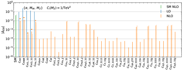
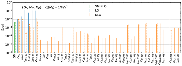
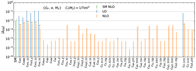
Figure 6: As in Figure 4, but for the decay $Z\to\tau\tau$.

• Figures 4, 5 and 6 show Eq. (84) for the NLO SM corrections as well as corrections appearing at LO and NLO in SMEFT when the choice $C_{i}=1\,{\rm TeV}^{-2}$ is made. They also show the large-$m_{t}$ limits of the NLO corrections in cases where top-loops contribute, and group the coefficients such that those appearing solely due to the choice of renormalisation scheme appear on the far right.

• In Tables 3, 4 and 5 we show the size of the NLO corrections to the SM and SMEFT coefficients which appear at tree-level in the different schemes, for the default scale choices.

• In Appendix B, we give results for the numerically most important contributions to the decay rates at LO and NLO in the SMEFT expansion, including uncertainties as estimated from scale variations.

The following subsections serve to explain and highlight the most noteworthy patterns emerging from these results.

5.1 $W\to\ell\nu$ decays

Figure 3: Representative virtual corrections for $W$ decay into leptons at NLO.

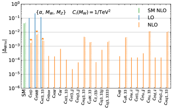
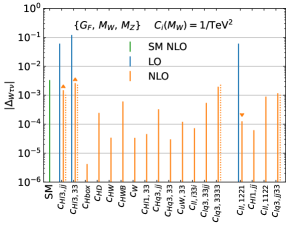
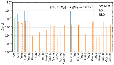
Figure 4: LO and NLO corrections $\Delta^{{\rm s}(i,j)}_{W\tau\nu}$, as defined in Eq. (84), for the decay $W\to\tau\nu$ in the three schemes. Note that “NLO” in the legends only refers to the NLO corrections and that we write superscripts in the Wilson coefficient names as $C_{Hq3}\equiv C_{Hq}^{(3)}$. The flavour indices $i$ and $j$ run over values $j\in 1,2$, and $i\in 1,2,3$. Operators which appear only through counterterms in a particular scheme are shown on the right. The dashed lines indicate the large-$m_{t}$ limit of the NLO corrections. For operators appearing at LO the orange triangles indicate if the sign of the NLO correction is the same as (triangle pointing up) or different from (triangle pointing down) the sign of the LO contribution.

The tree-level decay rate for $W\to\tau\nu$ decays, written in terms of $v_{T}$, takes the form

$$\Gamma_{W\tau\nu}^{(4,0)}+\Gamma_{W\tau\nu}^{(6,0)}=\frac{M_{W}}{12\pi}\frac{M_{W}^{2}}{v_{T}^{2}}\left(1+2v_{T}^{2}C_{\begin{subarray}{c}Hl\\ 33\end{subarray}}^{(3)}\right)\,.$$ (85)

Renormalisation-scheme dependence thus enters the result through the counterterms for $M_{W}$ and $v_{T}$.

The NLO decay rate is calculated by evaluating virtual corrections such as those shown in Figure 3, and then adding together with UV counterterms and real emission diagrams with an extra photon in the final state to get a finite result. The size of NLO SM corrections in the different schemes is easily understood using the large-$m_{t}$ analysis in Section 3.2. In that limit, the NLO corrections in the $\alpha_{\mu}$ scheme vanish, while those in $\alpha$ scheme are roughly $-3.4\%$, a pattern which agrees well with the full results in Table 3. The SM LEP scheme corrections in the large-$m_{t}$ limit are

$$\frac{\hat{M}_{W}}{12\pi}\frac{\hat{M}_{W}^{2}}{v_{\mu}^{2}}\left(1+\frac{3}{2}\frac{\hat{c}_{w}^{2}}{\hat{c}_{2w}}\frac{\Delta\rho_{t}^{(4,1)}}{v_{\mu}^{2}}\right)\approx\frac{\hat{M}_{W}}{12\pi}\frac{\hat{M}_{W}^{2}}{v_{\mu}^{2}}\left(1+0.02\right)\,,$$ (86)

so that the NLO correction is again very close to the result in the table. Note that in Eq. (86) we have consistently expressed all powers of the $W$ mass in terms of $\hat{M}_{W}$, whether they come from the 2-body phase space or directly from the amplitude, which accounts the factor of $3/2$ compared to Eq. (69). Absolute values of the decay rates at LO and NLO are given in Appendix B.1. In that notation, one finds the following ratios in the SM at NLO

$$\frac{\Gamma^{\alpha}_{W,\text{NLO}}}{\Gamma^{\alpha_{\mu}}_{W,\text{NLO}}}=0.992\,,\qquad\frac{\Gamma^{{\rm LEP}}_{W,\text{NLO}}}{\Gamma^{\alpha_{\mu}}_{W,\text{NLO}}}=1.003\,.$$ (87)

The first ratio agrees quite well with the estimate $G^{\rm NLO}_{F,\alpha}/G_{F}$ using Eq. (74), while the second is consistent with the estimate $(M_{W}^{\rm NLO})^{3}/M_{W}^{3}$ using Eq. (77). Once the NLO corrections are included the results between the schemes show (better than) percent-level agreement.

In Figure 4 the corrections in SMEFT are shown. The absolute size of the SMEFT corrections is determined by the choice $C_{i}={\rm TeV}^{-2}$. For that choice, SMEFT contributions are suppressed by $v_{\sigma}^{2}\times{\rm TeV}^{-2}\approx 6\%$, and are anywhere between 10% to below per-mille level of the SM tree-level result depending on the coefficient. The NLO SMEFT results contain a large number of Wilson coefficients. We have organised the coefficients in Figure 4 such that those appearing only due to the renormalisation of $v_{T}$ or $M_{W}$ up to NLO are separated out onto the right part of the figure, while those appearing also in the bare matrix elements or wavefunction renormalisation factors and thus common to all schemes are on the left. In the $\alpha_{\mu}$ scheme the coefficients $\Delta v_{\mu}^{(6,1,\mu)}$ appearing in Eq. (46) have a large overlap with those appearing in $W$-boson couplings, and as a result only four-fermion coefficients as well as those that modify $Z$ couplings to leptons, $C_{\begin{subarray}{c}Hl\\ jj\end{subarray}}^{(1)}$, with $j=1,2$, are particular to that scheme. In the $\alpha$ scheme, on the other hand, the renormalisation of $v_{T}$ brings in sensitivity to coefficients related to the renormalisation of $M_{Z}$ and $e$, which are listed in Eqs. (3.1) and (45). The LEP scheme is sensitive to the full set of coefficients contained in $\Delta r$, through the renormalisation of $M_{W}$, and therefore contains the overlap of the coefficients in the other two schemes. Taken as a whole, the number of Wilson coefficients contributing at NLO for the central scale choice is $39$ in the LEP scheme, $35$ in the $\alpha$ scheme and $25$ in the $\alpha_{\mu}$ scheme.

As in the SM, the numerically dominant NLO SMEFT corrections are related to top-quark loops. In the $\alpha$ and $\alpha_{\mu}$ schemes, the scheme-dependent corrections in the large-$m_{t}$ limit are nearly all contained in the factors $K_{W}$ given in Eqs. (3.2, 3.2). For the default input choices, the SMEFT contributions evaluate to

$$v_{\mu}^{2}K_{W}^{(6,0,\mu)} +K_{W}^{(6,1,\mu)}=v_{\mu}^{2}\bigg{[}\sum_{j=1,2}\bigg{(}-C_{\begin{subarray}{c}Hl\\ jj\end{subarray}}^{(3)}(1+0.0193)+0.0193C^{(3)}_{\begin{subarray}{c}lq\\ jj33\end{subarray}}\bigg{)}+C_{\begin{subarray}{c}ll\\ 1221\end{subarray}}(1+0.0)\bigg{]}\,,$$

$$v_{\alpha}^{2}K_{W}^{(6,0,\alpha)} +K_{W}^{(6,1,\alpha)}=v_{\alpha}^{2}\bigg{[}1.74C_{HD}\left(1-0.0275\right)+3.73C_{HWB}\left(1-0.0354\right)$$

$$+0.206\left(C_{\begin{subarray}{c}Hq\\ 33\end{subarray}}^{(1)}-C_{\begin{subarray}{c}Hu\\ 33\end{subarray}}\right)-0.0674C_{\begin{subarray}{c}Hq\\ 33\end{subarray}}^{(3)}-0.0727C_{\begin{subarray}{c}uB\\ 33\end{subarray}}-0.0334C_{\begin{subarray}{c}uW\\ 33\end{subarray}}\bigg{]}\,.$$ (88)

For coefficients appearing at LO, the NLO corrections are the second term in the parentheses, facilitating a comparison with Table 3. Results also for coefficients first appearing at NLO can be found in Eq. (144) and Eq. (146). We see the large-$m_{t}$ limit corrections are a good approximation to the full ones. Interestingly, for the coefficients appearing at LO, there is no large hierarchy between the size of NLO corrections in the $\alpha$ scheme compared to the $\alpha_{\mu}$ scheme, even though the analytic result for $K_{W}^{(6,1,\alpha)}$ contains 4 (3) inverse powers of $s_{w}$ in the case of $C_{HD}$ ($C_{HWB}$). In fact, the largest corrections are from $C_{\begin{subarray}{c}Hq\\ 33\end{subarray}}^{(1)}$ and $C_{\begin{subarray}{c}Hu\\ 33\end{subarray}}$, which appear only due to the scale-dependent logarithmic terms from Eq. (3.2). This illustrates the important point that, unlike the SM, the NLO corrections are strongly scale dependent in SMEFT.

The SMEFT corrections in the LEP scheme can be derived from results in the $\alpha_{\mu}$ scheme using Eq. (33) to write $M_{W}$ in terms of $\hat{M}_{W}$. The expansion coefficients arising after converting the factor of $M_{W}^{2}$ in the large-$m_{t}$ limit, $\hat{K}_{W}^{(6,j,\mu)}$, were given in Eqs. (70, 3.2). In order to calculate the decay rate one must also write the factor of $M_{W}$ arising from 2-body phase space in terms of $\hat{M}_{W}$. We have checked that after doing so the large-$m_{t}$ limit corrections to the coefficients appearing in $\hat{K}_{W}$ are a good numerical approximation to the full ones.

In addition to the corrections related to the flavour-independent corrections, there are also contributions from the coefficient $C_{\begin{subarray}{c}Hl\\ 33\end{subarray}}^{(3)}$, which specifically modifies the $\tau\nu W$ coupling. The large-$m_{t}$ limit correction to $\Delta^{{\rm LEP}(6,1)}_{W,t}$ due to this coefficient is given by

$$-2\Delta\rho_{t}^{(4,1)}C_{\begin{subarray}{c}Hl\\ 33\end{subarray}}^{(3)}\left(1+2\ln\frac{\mu^{2}}{m_{t}^{2}}\right)\left(1+3\hat{\Delta}_{W,t}^{(4,1,\mu)}\right)\,.$$ (89)

The corresponding results in the $\alpha$ and $\alpha_{\mu}$ schemes are obtained from the above by setting $\hat{\Delta}_{W,t}^{(4,1,\mu)}$ to zero. Numerically, one finds that the NLO corrections to $C_{\begin{subarray}{c}Hl\\ 33\end{subarray}}^{(3)}$ are about 4% in the LEP scheme, and 2% in the $\alpha$ and $\alpha_{\mu}$ schemes, in rough agreement with Table 3. Compared to the other schemes, the NLO corrections to the coefficients appearing at tree-level in the LEP scheme show a rather irregular pattern due to the complicated dependence on the Weinberg angle.

While the size of the NLO corrections studied above is rather scale dependent, the sum of the LO and NLO contributions is independent of the scale (up to uncalculated NNLO terms in the SMEFT expansion) and is thus much less sensitive. To study this effect in detail, in Appendix B.1 we give numerical results in the three schemes including scale variations at LO and NLO. It is seen that in SMEFT, the dominant NLO corrections are typically within the uncertainties of the LO calculation as estimated through scale variations, and that the scale uncertainties in the NLO results are substantially smaller than in the LO ones.

$W\rightarrow\tau\nu$	SM	$C_{HD}$	$C_{HWB}$	$C^{(3)}_{\begin{subarray}{c}Hl\\ jj\end{subarray}}$	$C_{\begin{subarray}{c}ll\\ 1221\end{subarray}}$	$C^{(3)}_{\begin{subarray}{c}Hl\\ 33\end{subarray}}$
$\alpha$	$-4.2\%$	$-1.7\%$	$-3.0\%$	—	—	$2.2\%$
$\alpha_{\mu}$	$-0.3\%$	—	—	$2.5\%$	$-0.2\%$	$2.2\%$
LEP	$2.0\%$	$8.1\%$	$3.2\%$	$5.1\%$	$2.5\%$	$4.6\%$

Table 3: NLO corrections to prefactors of LO Wilson coefficients in the three schemes. Negative corrections indicate a reduction in the magnitude of the numerical coefficient of a given Wilson coefficient. The flavour index $j$ refers to $j\in 1,2$.

5.2 $h\to b\bar{b}$ decays

$h\to b\bar{b}$		SM	$C_{H\Box}$	$C_{HD}$	$C_{\begin{subarray}{c}dH\\ 33\end{subarray}}$	$C_{HWB}$	$C_{\begin{subarray}{c}Hl\\ jj\end{subarray}}^{(3)}$	$C_{\begin{subarray}{c}ll\\ 1221\end{subarray}}$
	NLO QCD	20.3%	20.3%	20.3%	20.3%	20.3%	-	-
$\alpha$	NLO EW	-5.2 %	2.1%	-11.0%	4.2%	-6.7%	-	-
	NLO correction	15.1%	22.4%	9.3%	24.5%	13.6%	-	-
	NLO QCD	20.3%	20.3%	20.3%	20.3%	-	20.3%	20.3%
$\alpha_{\mu}$	NLO EW	-0.8 %	2.1%	2.0%	1.9%	-	0.9%	-0.8%
	NLO correction	19.5%	22.4%	22.3%	22.2%	-	21.2%	19.5%
	NLO QCD	20.3%	20.3%	20.3%	20.3%	-	20.3%	20.3%
LEP	NLO EW	-0.7 %	2.1%	1.6%	1.9%	-	0.7%	-0.9%
	NLO correction	19.5%	22.3%	21.9%	22.2%	-	21.0%	19.3%

Table 4: NLO corrections to prefactors of LO Wilson coefficients in the three schemes, split into QCD and EW corrections. The flavour index $j$ refers to $j\in 1,2$.

The tree-level decay rate for $h\to b\bar{b}$ decay is given by

$$\Gamma_{hb\bar{b}}^{(4,0)}+\Gamma_{hb\bar{b}}^{(6,0)}=\frac{3m_{b}^{2}M_{h}}{8\pi v_{T}^{2}}\left[1+v_{T}^{2}\left(2C_{H\Box}-\frac{1}{2}C_{HD}-\sqrt{2}\frac{v_{T}}{m_{b}}C_{\begin{subarray}{c}dH\\ 33\end{subarray}}\right)\right]\,.$$ (90)

The decay $h\to b\bar{b}$ has two important differences with respect to the decays $W\to\ell\nu$ and $Z\to\ell\ell$ (to be discussed in Section 5.3). First, we retain the $b$-quark mass and, second, the strong coupling $\alpha_{s}(\mu)$ plays a role in the results already at NLO. The Higgs mass $M_{h}$ is evaluated on-shell, but the NLO corrections do not involve its counterterm since it appears through phase space rather than through the amplitude. Therefore, the input-scheme dependence to NLO arises mainly through the counterterm for $v_{T}$.

The decay $h\to b\bar{b}$ receives both QCD and EW corrections at NLO. The two effects are additive and to study the EW input scheme dependence of the results it is useful to quote the QCD and EW corrections separately, as in Table 4. To this order, the QCD corrections are scheme independent. In the $\alpha$ scheme the EW corrections are rather large and depend heavily on the Wilson coefficient considered, ranging from -11% to 4% and thus inducing significant shifts to QCD alone, while in the $\alpha_{\mu}$ and LEP schemes the corrections are smaller are more uniform.

We can understand the qualitative features of the NLO EW corrections using the large-$m_{t}$ limit. To this end, we use Eq. (3.2) to write the NLO decay rate in this limit as

$$\Gamma^{s}_{hb\bar{b}}\bigg{|}_{m_{t}\to\infty}=\frac{3m_{b}^{2}M_{h}}{8\pi v_{\sigma}^{2}}\bigg{[} 1+v_{\sigma}^{2}\left(K_{h}^{(6,0)}+K_{W}^{(6,0,\sigma)}\right)+\frac{1}{v_{\sigma}^{2}}\left(K_{h}^{(4,1)}+K_{W}^{(4,1,\sigma)}\right)$$

$$+K_{h}^{(6,1)}+\Delta K_{h}^{(6,1,\sigma)}\bigg{]}\,,$$ (91)

where $K_{h}^{(6,0)}$ is the SMEFT contribution in Eq. (90), and the scheme-dependent part of the NLO SMEFT correction is

$$\Delta K_{h}^{(6,1,\sigma)}=K_{W}^{(6,1,\sigma)}+2K_{h}^{(4,1)}K_{W}^{(6,0,\sigma)}+\frac{1}{\sqrt{2}}\frac{v_{\sigma}}{m_{b}}K_{W}^{(4,1,\sigma)}C_{\begin{subarray}{c}dH\\ 33\end{subarray}}\,.$$ (92)

Large-$m_{t}$ limit results in the $\alpha$ scheme have been given previously in Cullen:2019nnr , while those in the $\alpha_{\mu}$ scheme can be extracted from Gauld:2015lmb . We make use of those results in what follows, thus employing the “vanishing gauge coupling limit”, which in this case amounts to taking the limit $M_{W}\ll M_{h}$ in addition to $m_{t}\to\infty$. The LEP and $\alpha_{\mu}$ scheme results are identical in this limit.

In the SM, the scheme-independent NLO correction in the large-$m_{t}$ limit is given by

$$\frac{1}{v_{\sigma}^{2}}K_{h}^{(4,1)}=\frac{1}{3v_{\sigma}^{2}}\Delta\rho_{t}^{(4,1)}\left(1+\frac{7(N_{c}-3)}{3}\right)\approx 0.003\,.$$ (93)

It follows from the discussion in Section 3.2 that the large-$m_{t}$ limit corrections in the $\alpha_{\mu}$ scheme are tiny, while those in the $\alpha$ scheme are well approximated by $K_{W}^{(4,1,\alpha)}\approx-3.4\%$. Clearly, this mimics the features of the exact NLO EW corrections given in Table 4.

In SMEFT, the scheme-independent NLO correction in the large-$m_{t}$ limit is given by

$$\frac{K_{h}^{(6,1)}}{K_{h}^{(4,1)}} =C_{HD}\left(-1+6L_{t}\right)+2\sqrt{2}\frac{M_{W}}{m_{t}}\left(-7+6L_{t}\right)C_{\begin{subarray}{c}uW\\ 33\end{subarray}}+4\left(1+6L_{t}\right)C^{(3)}_{\begin{subarray}{c}Hq\\ 33\end{subarray}}$$

$$+\frac{3}{2\sqrt{2}}\frac{v_{\sigma}}{m_{b}}\left(-1+10L_{t}\right)C_{\begin{subarray}{c}dH\\ 33\end{subarray}}+\dots\,,$$ (94)

where $L_{t}=\ln(\mu^{2}/m_{t}^{2})$ and we have set $N_{c}=3$. The $\dots$ refer to Wilson coefficients which contain no overlap with those appearing in the scheme-dependent pieces in Eq. (92). In the $\alpha$ scheme the numerical value of the NLO corrections at $\mu=M_{h}$ is

$$\frac{1}{v_{\alpha}^{2}}\left(K_{h}^{(6,1)}+\Delta K_{h}^{(6,1,\alpha)}\right)=\bigg{\{}-C_{HD}(1.6+9.7)+(0.0-17)C_{HWB}$$

$$-(3.7+6.8)C_{\begin{subarray}{c}Hq\\ 33\end{subarray}}^{(3)}+(0.0-8.8)(C_{\begin{subarray}{c}Hu\\ 33\end{subarray}}-C_{\begin{subarray}{c}Hq\\ 33\end{subarray}}^{(1)})+(0.0-3.1)C_{\begin{subarray}{c}uB\\ 33\end{subarray}}+(-4.6+0.42)C_{\begin{subarray}{c}uW\\ 33\end{subarray}}$$

$$-\frac{\sqrt{2}v_{\alpha}}{{m_{b}}}\left(1.8+1.7\right)C_{\begin{subarray}{c}dH\\ 33\end{subarray}}\bigg{\}}\times 10^{-2}+\dots\,,$$ (95)

where the $\dots$ refer to coefficients not appearing in $\Delta K_{W}^{(6,1,\alpha)}$, and the order of the numbers inside the parentheses multiplying the Wilson coefficients on the right-hand side of the above equation matches the order of the two terms on the left-hand side. In most cases the scheme-dependent parts contained in $\Delta K_{W}^{(6,1,\alpha)}$ dominate over the scheme-independent ones. For coefficients not appearing already at NLO, one can verify that the results above are close to the exact NLO results in Eq. (153). Combined with the LO result in Eq. (152), one infers NLO EW corrections of $-9\%$ for $C_{HD}$, $-5\%$ for $C_{HWB}$ in the $\alpha$ scheme. In the $\alpha_{\mu}$ scheme, one has

$$\frac{1}{v_{\mu}^{2}}\Delta K_{h}^{(6,1,\mu)} =\bigg{\{}0.6C_{\begin{subarray}{c}ll\\ 1221\end{subarray}}+\sum_{j=1,2}\bigg{[}-0.9C_{\begin{subarray}{c}Hl\\ jj\end{subarray}}^{(3)}+0.3C^{(3)}_{\begin{subarray}{c}lq\\ jj33\end{subarray}}\bigg{]}\bigg{\}}\times 10^{-2}\,.$$ (96)

Contributions from $C_{HWB}$ are completely absent in the $\alpha_{\mu}$ scheme, while the NLO EW correction to $C_{HD}$ from the above result and Eq. (154) is $3$% in the large-$m_{t}$ limit. This explains the pattern of results seen for these coefficients in Table 4. It makes clear that in this case factors of $K_{W}^{(i,j,\alpha)}$ work much the same in SMEFT as in the SM, producing sizeable NLO EW corrections compared to the $\alpha_{\mu}$ scheme.

The full set of NLO corrections in the different schemes is shown in Figure 5. In the numerical results in Appendix B.2 we follow Cullen:2019nnr and leave in symbolic form enhancement factors of $m_{b}/v_{\sigma}$ which disappear when Minimal Flavour Violation is assumed. We have not done this in the figure, which explains, for instance, the very large contribution from $C_{\begin{subarray}{c}dH\\ 33\end{subarray}}$. In contrast to the case of $W$ decay, in some cases there are large differences between the large-$m_{t}$ limit and full corrections; this occurs when a Wilson coefficient receives both EW and QCD corrections, the latter invariably being the larger effect. From the perspective of EW input-scheme dependent corrections, the most important feature of the figure is the number of Wilson coefficients appearing. In particular, there are far more in the $\alpha$ scheme, 42 in total, than in the $\alpha_{\mu}$ or LEP schemes, both of which receive contributions from the same 29 Wilson coefficients. The main reason is that the renormalisation of $v_{T}$ in the $\alpha$ scheme involves the large set of flavour-specific couplings to fermions identified given in Eq. (3.1), while in the $\alpha_{\mu}$ and LEP schemes $M_{Z}$ does not enter the tree-level amplitude and many of these coefficients are therefore absent.

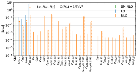
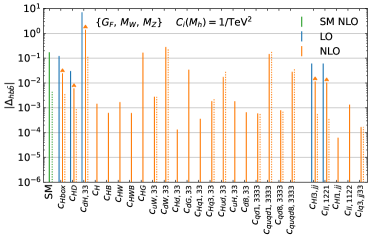
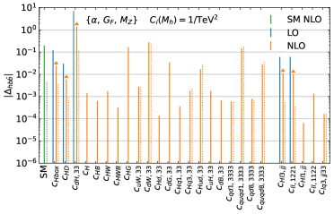
Figure 5: As in Figure 4, but for the decay $h\to b\bar{b}$.

5.3 $Z\to\ell\ell$ decays

The tree-level decay rate for $Z\to\tau\tau$ decay, written in terms of $v_{T}$, takes the form

$$\Gamma_{Z\tau\tau}^{(4,0)}+\Gamma_{Z\tau\tau}^{(6,0)} =\frac{M_{Z}}{24\pi}\bigg{\{}\left[\frac{M_{Z}^{2}}{v_{T}^{2}}\left(1-\frac{v_{T}^{2}}{2}C_{HD}\right)\right]\left(g_{\tau}^{(4,0)}+v_{T}^{2}g_{\tau}^{(6,0)}\right)$$

$$+2M_{Z}^{2}\left[c_{2w}\left(C^{(1)}_{\begin{subarray}{c}Hl\\ 33\end{subarray}}+C^{(3)}_{\begin{subarray}{c}Hl\\ 33\end{subarray}}\right)-2s_{w}^{2}C_{\begin{subarray}{c}He\\ 33\end{subarray}}\ \right]\bigg{\}}\,,$$ (97)

where

$$g_{\tau}^{(4,0)} =1-4s_{w}^{2}+8s_{w}^{4}\,,$$

$$g_{\tau}^{(6,0)} =2\left(1-4s_{w}^{2}\right)\left(c_{w}^{2}C_{HD}+2c_{w}s_{w}C_{HWB}\right)\,.$$ (98)

The term inside the square brackets in the first line of Eq. (5.3) is independent of the fermion species into which the $Z$ decays and was considered in Eq. (61). The function $g_{\tau}$ depends on the charge and weak isospin of the $\tau$ lepton, and the terms on second line are specific to $Z\tau\tau$ couplings in SMEFT. The LO decay rate depends on the full set of parameters $M_{W},M_{Z},v_{T}$, and so scheme-dependent corrections involve the full set of coefficients identified in Section 3.1.

The NLO decay rates in the three schemes are shown in Figure 6. In the $\alpha$ scheme the set of coefficients appearing in the renormalisation of $v_{T}$ is the same as that for renormalising $M_{Z}$ and $M_{W}$, so it does not introduce any unique coefficients at NLO. In the LEP and $\alpha_{\mu}$ schemes, on the other hand, the renormalisation of $v_{T}$ introduces a set of 4-fermion coefficients shown on the right-hand side of the figure that would not otherwise appear in the decay rate. In this case the number of coefficients appearing at NLO is quite large: 63 in the $\alpha$ scheme, and 67 in the $\alpha_{\mu}$ and LEP schemes.

In order to understand the dominant corrections we study the large-$m_{t}$ limit. Let us first consider the corrections to the SMEFT coefficients specific to $Z\tau\tau$ couplings, given in the second line of Eq. (5.3). In order to evaluate them in the three schemes, we can use

$$\Delta M_{Z,t}^{(4,1)}=\hat{\Delta}M_{Z,t}^{(4,1,\mu)}=-\Delta\rho_{t}^{(4,1)}\ln\frac{\mu^{2}}{m_{t}^{2}}+\dots\,,$$ (99)

where the $\dots$ signify tadpole contributions which cancel against those in the bare matrix elements. Along with the LEP scheme result

$$\hat{\Delta}s_{w,t}^{(4,1,\mu)}=-\frac{\hat{c}_{w}^{2}}{2\hat{c}_{2w}}\Delta\rho_{t}^{(4,1)}\approx-0.7\Delta\rho_{t}^{(4,1)}\approx-0.4\Delta s_{w,t}^{(4,1,\mu)}\,,$$ (100)

it is then easy to show that in the large-$m_{t}$ limit we can replace the tree-level expressions involving $C_{\begin{subarray}{c}He\\ 33\end{subarray}}$ by

$$M_{Z}^{2}s_{w}^{2}C_{\begin{subarray}{c}He\\ 33\end{subarray}}\to M_{Z}^{2}s_{w}^{2}C_{\begin{subarray}{c}He\\ 33\end{subarray}}\left(1+\frac{1}{v_{\mu}^{2}}\left[\frac{c_{w}^{2}}{s_{w}^{2}}-2\ln\frac{\mu^{2}}{m_{t}^{2}}\right]\Delta\rho_{t}^{(4,1)}\right)\approx M_{Z}^{2}s_{w}^{2}C_{\begin{subarray}{c}He\\ 33\end{subarray}}\left(1+0.06\right)\,,$$

$$M_{Z}^{2}s_{w}^{2}C_{\begin{subarray}{c}He\\ 33\end{subarray}}\to M_{Z}^{2}\hat{s}_{w}^{2}C_{\begin{subarray}{c}He\\ 33\end{subarray}}\left(1+\frac{1}{v_{\mu}^{2}}\left[-\frac{\hat{c}_{w}^{2}}{\hat{c}_{2w}}-2\ln\frac{\mu^{2}}{m_{t}^{2}}\right]\Delta\rho_{t}^{(4,1)}\right)\approx M_{Z}^{2}\hat{s}_{w}^{2}C_{\begin{subarray}{c}He\\ 33\end{subarray}}\left(1+0.01\right)\,,$$

where the first result is for the $\alpha_{\mu}$ (or $\alpha$ scheme after $\mu\to\alpha$) and the second line is for the LEP scheme. The results are a good approximation to the exact ones shown in Table 5. The fairly large difference between the LEP and $\alpha_{\mu}$ scheme makes clear that the corrections can be quite sensitive to the exact dependence on e.g. $s_{w}$ in the tree-level results. We have checked that the corrections to the remaining coefficients appearing in the second line of Eq. (5.3) are also well-approximated by the large-$m_{t}$ limit.

The NLO corrections related to the first line of Eq. (5.3) are more complicated. To study them, we first note that the large-$m_{t}$ limit corrections to the function $g_{\tau}$ can be written in the $\alpha$ and $\alpha_{\mu}$ schemes as

$$g_{\tau}=g_{\tau}^{(4,0)}+v_{\sigma}^{2}g_{\tau}^{(6,0)}+\frac{1}{v_{\sigma}^{2}}g_{\tau}^{(4,1)}+g_{\tau}^{(6,1)}+\left(K_{W}^{(6,0,\sigma)}g_{\tau}^{(4,1)}-K_{W}^{(4,1,\sigma)}g_{\tau}^{(6,0)}\right)\,.$$ (102)

The scheme-independent function $g_{\tau}^{(4,1)}$ is obtained by replacing $s_{w}\to s_{w}(1+\Delta s_{w})$ and isolating the SM corrections; it thus reads

$$g_{\tau}^{(4,1)}=-4c_{w}^{2}(1-4s_{w}^{2})\Delta\rho_{t}^{(4,1)}\,.$$ (103)

The function $g_{\tau}^{(6,1)}$ is obtained in the same way, except for in that case one must also include corrections from $Z-\gamma$ mixing to get a finite and tadpole-free result. The explicit result is

$$g_{\tau}^{(6,1)} =-\frac{1}{2}\dot{g}_{\tau}^{(6,0)}\ln\frac{\mu^{2}}{m_{t}^{2}}+g_{\tau}^{(4,1)}\left(-\frac{C_{HWB}}{2c_{w}s_{w}}+2C_{\begin{subarray}{c}Hq\\ 33\end{subarray}}^{(3)}-2\sqrt{2}\frac{M_{W}}{M_{T}}C_{\begin{subarray}{c}uW\\ 33\end{subarray}}\right)$$

$$-12c_{2w}\Delta\rho_{t}^{(4,1)}\left(c_{w}^{2}C_{HD}+2c_{w}s_{w}C_{HWB}\right)\,,$$ (104)

where

$$\dot{g}_{\tau}^{(6,0)}=-4g_{\tau}^{(4,1)}\bigg{[}C_{HD}+\frac{s_{w}}{c_{w}}C_{HWB}+2C_{\begin{subarray}{c}Hq\\ 33\end{subarray}}^{(1)}-2C_{\begin{subarray}{c}Hu\\ 33\end{subarray}}-\frac{\sqrt{2}s_{w}}{c_{w}^{2}}\frac{M_{W}}{m_{t}}\left(c_{w}C_{\begin{subarray}{c}uB\\ 33\end{subarray}}+\frac{5}{3}s_{w}C_{\begin{subarray}{c}uW\\ 33\end{subarray}}\right)\bigg{]}\,.$$ (105)

We can now obtain the NLO corrections to the first line of Eq. (5.3) in the large-$m_{t}$ limit in the $\alpha$ scheme through the replacement

$$\frac{M_{Z}^{2}}{v_{T}^{2}}\left(1-\frac{v_{T}^{2}}{2}C_{HD}\right)\left(g_{\tau}^{(4,0)}+v_{T}^{2}g_{\tau}^{(6,0)}\right)\to\frac{M_{Z}^{2}}{v_{\alpha}^{2}}\left(g_{\tau}^{(4,0)}+v_{\alpha}^{2}K_{Z}^{(6,0,\alpha)}+\frac{1}{v_{\alpha}^{2}}K_{Z}^{(4,1,\alpha)}+K_{Z}^{(6,1,\alpha)}\right)\,,$$ (106)

where the coefficients $K_{Z}$ are obtained by expanding out Eqs. (61) and (102). The SM result in the $\alpha$ scheme is then given by

$$g_{\tau}^{(4,0)}+\frac{1}{v_{\alpha}^{2}}K_{Z}^{(4,1,\alpha)} =g_{\tau}^{(4,0)}+\frac{1}{v_{\alpha}^{2}}\left(g_{\tau}^{(4,0)}K_{W}^{(4,1,\alpha)}+g_{\tau}^{(4,0)}k_{Z}^{(4,1)}+g_{\tau}^{(4,1)}\right)$$

$$\approx g_{\tau}^{(4,0)}(1-0.034+0.009-0.006)\,,$$ (107)

where the order of numerical terms on the second line matches the first, and $g_{\tau}^{(4,0)}\approx 0.51$. In the $\alpha_{\mu}$ scheme $K_{W}^{(4,1,\mu)}=0$, and in the LEP scheme one replaces $g_{\tau}^{(4,1)}\to-\frac{s_{w}^{2}}{c_{2w}}g_{\tau}^{(4,1)}\approx-0.40g_{\tau}^{(4,1)}$. This accounts for the SM corrections in the $\alpha$ and $\alpha_{\mu}$ schemes given in Table 5, which as in Higgs and $W$ decay follows the pattern identified in Section 3.2.

Turning to SMEFT, the LO corrections in the $\alpha$ scheme are contained in

$$K_{Z}^{(6,0,\alpha)} =g_{\tau}^{(4,0)}K_{W}^{(6,0,\alpha)}-g_{\tau}^{(4,0)}\frac{C_{HD}}{2}+g_{\tau}^{(6,0)}$$

$$\approx g_{\tau}^{(4,0)}K_{W}^{(6,0,\alpha)}-0.25C_{HD}+\left(0.17C_{HD}+0.18C_{HWB}\right)\,$$

$$\approx 0.80C_{HD}+2.0C_{HWB}\,,$$ (108)

where the order of the terms on the second line matches that in the first. In the $\alpha_{\mu}$ scheme one replaces $\alpha\to\mu$ in the above equation; in that case it is clear that the tree-level contributions from $C_{HD}$ and $C_{HWB}$ are quite small, since $K_{W}^{(6,0,\mu)}$ contains neither of these coefficients. At NLO in SMEFT, we can write

$$K_{Z}^{(6,1,\sigma)}=K_{Z}^{(6,1)}+\Delta K_{Z}^{(6,1,\sigma)}\,,$$ (109)

where the first term is independent of the scheme. In terms of component objects, one finds

$$\Delta K_{Z}^{(6,1,\sigma)} =g_{\tau}^{(4,0)}K_{W}^{(6,1,\sigma)}+2g_{\tau}^{(4,0)}K_{W}^{(6,0,\sigma)}k_{Z}^{(4,1)}+2g_{\tau}^{(4,1)}K_{W}^{(6,0,\sigma)}\,,$$

$$K_{Z}^{(6,1)} =g_{\tau}^{(4,0)}k_{Z}^{(6,1)}+g_{\tau}^{(6,1)}+g_{\tau}^{(6,0)}k_{Z}^{(4,1)}+g_{\tau}^{(4,1)}k_{Z}^{(6,0)}\,.$$ (110)

One can use explicit expressions for the component functions given above to evaluate these numerically. As an example, let us consider the contributions from $C_{HWB}$ and $C_{HD}$ in the $\alpha_{\mu}$ scheme. These are contained solely in the scheme-independent factor, which at the scale $\mu=M_{Z}$

$$\frac{1}{v_{\mu}^{2}}K_{Z}^{(6,1)}=-0.049C_{HD}-0.042C_{HWB}+\dots$$ (111)

where the $\dots$ refer to contributions from other $C_{i}$, which are less than 1% in the units above. Comparing with the second line of Eq. (5.3), this implies NLO corrections of 60% for $C_{HD}$ and $-20\%$ for $C_{HWB}$, which are indeed close to the huge corrections in the exact results in Table 5. In the $\alpha$ scheme these coefficients also contribute through the scheme dependent piece. The numerical result is

$$\frac{1}{v_{\alpha}^{2}}\Delta K_{Z}^{(6,1,\alpha)}= -0.027C_{HD}-0.064C_{HWB}$$ (112)

$$+g_{\tau}^{(4,0)}\left[0.17C_{\begin{subarray}{c}Hq\\ 33\end{subarray}}^{(1)}-0.17C_{\begin{subarray}{c}Hu\\ 33\end{subarray}}-0.067C_{\begin{subarray}{c}Hq\\ 33\end{subarray}}^{(3)}-0.061C_{\begin{subarray}{c}uB\\ 33\end{subarray}}-0.023C_{\begin{subarray}{c}uW\\ 33\end{subarray}}\right]\,.$$

Even though the contributions on the first line contain up to four (three) inverse powers of $s_{w}$ in the case of $C_{HD}$ ($C_{HWB}$), there is no clear hierarchy compared to the scheme-independent pieces in Eq. (111). Combining them with the LO numbers in Eq. (5.3), we account for the pattern seen in Table 5. Clearly, this pattern is quite complicated and is not driven by the scheme-dependent factors $K_{W}$ as in the SM. On the other hand, the coefficients on the second line only appear through $K_{W}^{(6,1,\alpha)}$, and as seen from the exact results in Eq. (159) we see that this factor indeed absorbs the dominant corrections from them, much like $K_{W}^{(4,1,\alpha)}$ in the SM.

The LEP scheme results can be obtained from those in the $\alpha_{\mu}$ scheme by employing Eq. (2.3). In the large-$m_{t}$ limit the only non-trivial conversions are on the functions $g_{\tau}$, which contain $M_{W}$ dependence already at tree level. For instance, calling the LEP-scheme functions $\hat{g}_{\tau}$, we have the LO SMEFT result

$$\hat{g}_{\tau}^{(6,0)}=4(1-4s_{w}^{2})\frac{c_{w}^{2}s_{w}^{2}}{c_{2w}}\left[\frac{1}{2}C_{HD}+\frac{1}{c_{w}s_{w}}C_{HWB}-K_{W}^{(6,0,\mu)}\right]\,,$$ (113)

and the LEP-scheme version of Eq. (5.3) becomes

$$\hat{K}_{Z}^{(6,0,\mu)}= \hat{g}_{\tau}^{(4,0)}K_{W}^{(6,0,\mu)}-\hat{g}_{\tau}^{(4,0)}\frac{C_{HD}}{2}+\hat{g}_{\tau}^{(6,0)}$$

$$\approx-0.29C_{HD}-0.21C_{HWB}-0.59\left(\sum_{j=1,2}C^{(3)}_{\begin{subarray}{c}Hl\\ jj\end{subarray}}-C_{\begin{subarray}{c}ll\\ 1221\end{subarray}}\right)\,.$$ (114)

Compared to the $\alpha_{\mu}$ scheme, the LO result for the coefficient $C_{HD}$ is significantly larger, and those from the operators contained in $K_{W}^{(6,0,\mu)}$ are slightly smaller, which roughly explains the pattern for those coefficients seen in LEP scheme results Table 5. The result for $C_{HWB}$ is slightly increased, but remains small and for that reason still receives a substantial NLO correction.

We have derived the complete large-$m_{t}$ limit results and verified that they provide a good approximation to the full one, but the explicit expression for the function $\hat{g}^{(6,1,\mu)}_{\tau}$ is somewhat lengthy and we do not reproduce it here. In Section B.3 we show detailed LO and NLO results including uncertainties estimated from scale variations. It is clear that in cases where the NLO corrections are large, namely for certain operators in the $\alpha_{\mu}$ and the LEP schemes, the uncertainties are underestimated, while in the $\alpha$-scheme the uncertainty estimates are more reliable. This example highlights very clearly that the issue of NLO corrections in SMEFT is considerably more scheme and process-dependent than in the SM. The general rule that NLO corrections to weak decays are smaller in the LEP and $\alpha_{\mu}$ schemes than in the $\alpha$ scheme familiar from the SM does not transfer over to SMEFT.

$Z\rightarrow\tau\tau$	SM	$C_{HD}$	$C_{HWB}$	$C_{\begin{subarray}{c}He\\ 33\end{subarray}}$	$C^{(1)}_{\begin{subarray}{c}Hl\\ 33\end{subarray}}$	$C^{(3)}_{\begin{subarray}{c}Hl\\ 33\end{subarray}}$	$C^{(3)}_{\begin{subarray}{c}Hl\\ jj\end{subarray}}$	$C_{\begin{subarray}{c}ll\\ 1221\end{subarray}}$
$\alpha$	$-4.0\%$	$-10.6\%$	$-5.4\%$	$7.7\%$	$0.3\%$	$-0.5\%$	—	—
$\alpha_{\mu}$	$<0.1\%$	$71.1\%$	$-27.2\%$	$7.6\%$	$0.1\%$	$-0.4\%$	$2.9\%$	$0.6\%$
LEP	$1.0\%$	$7.8\%$	$17.4\%$	$2.0\%$	$4.7\%$	$4.2\%$	$6.9\%$	$4.5\%$

Table 5: NLO corrections to prefactors of LO Wilson coefficients in the three schemes. Negative corrections indicate a reduction in the magnitude of the numerical coefficient of a given Wilson coefficient, while $<0.1\%$ indicates changes below $0.1\%$, both positive and negative. The flavour index $j$ refers to $j\in 1,2$.

6 Universal corrections in SMEFT

A recurring theme of the previous sections was that EW corrections are dominated by top loops. While the numerical patterns in EW input-scheme dependent top-loop corrections in the SM are quite regular, those in SMEFT are more process and Wilson-coefficient dependent. The purpose of this section is to show that the dominant scheme-dependent EW corrections in SMEFT can nonetheless be taken into account by a certain set of simple substitutions in the LO results, similarly to the well-studied case of the SM.

Let us begin the discussion with the SM, where an important feature is that weak vertices in the $\alpha$ scheme receive corrections proportional to $\Delta r_{t}^{(4,1)}$, related to the renormalisation of $v_{T}$. It is simple to resum such corrections to all orders in perturbation theory. Using the large-$m_{t}$ limit result in Eq. (51), and keeping for the moment only the $\Delta r_{t}^{(4,1)}$ terms (i.e. terms enhanced in the limit $c_{w}^{2}/s_{w}^{2}\gg 1$, in which case the $\Delta M_{W,t}$ piece is subleading), we have

$$\frac{1}{v_{T,0}^{2}} \approx\frac{1}{v_{\alpha}^{2}}\left[1+\frac{1}{v_{T,0}^{2}}\Delta r_{t}^{(4,1)}\right]\approx\frac{1}{v_{\alpha}^{2}}\left[1+\frac{1}{v_{\alpha}^{2}}\Delta r_{t}^{(4,1)}+\frac{1}{v_{\alpha}^{2}v_{T,0}^{2}}\left(\Delta r_{t}^{(4,1)}\right)^{2}+\dots\right]$$

$$=\frac{1}{v_{\alpha}^{2}}\left[1-\frac{1}{v_{\alpha}^{2}}\Delta r_{t}^{(4,1)}\right]^{-1}\equiv\frac{1}{\tilde{v}_{\alpha}^{2}}\,.$$ (115)

This resums the $\Delta r_{t}^{(4,1)}$ terms to all orders. Adding back the subleading terms away from the double limit $m_{t},\,c_{w}^{2}/s_{w}^{2}\gg 1$ by matching with the one-loop result yields

$$\frac{1}{v_{T,0}^{2}}=\frac{1}{\tilde{v}_{\alpha}^{2}}\left[1-\frac{1}{\tilde{v}_{\alpha}^{2}}\left(\Delta v_{\alpha}^{(4,1,\alpha)}+\Delta r_{t}^{(4,1)}\right)\right]\,.$$ (116)

Expressing the counterterm for $v_{T}$ as an expansion in $\tilde{v}_{\alpha}$ rather than $v_{\alpha}$ will obviously lead to a quicker convergence between orders. For example, the SM prediction to NLO for the derived quantity $G_{F}$ in such a “$\tilde{\alpha}$ scheme” is

$$G_{F,\tilde{\alpha}}^{\rm NLO} =\frac{1}{\sqrt{2}\tilde{v}_{\alpha}^{2}}\left[1+\frac{1}{\tilde{v}_{\alpha}^{2}}\left(\Delta r^{(4,1)}-\Delta r_{t}^{(4,1)}\right)\right]\,.$$ (117)

Numerically, including uncertainties from scale variation using the procedure described in Section 4,

$$\frac{G_{F,\tilde{\alpha}}^{\text{LO}}}{G_{F}}=1.000^{+0.007}_{-0.007}\,,\qquad\frac{G_{F,\tilde{\alpha}}^{\text{NLO}}}{G_{F}}=0.994^{+0.000}_{-0.000}\,,$$ (118)

where $G_{F,\tilde{\alpha}}^{\text{LO}}$ refers to the first term in Eq. (117). This shows considerably improved convergence compared to the fixed-order $\alpha$ scheme expression in Eq. (72), and scale variations in the LO result give a good estimate of the NLO corrections.

To the best of our knowledge, a resummation of the type described above was first derived in Consoli:1989fg , at the level of the $W$-boson mass in the LEP scheme (and also including subleading two-loop terms in the limit $s_{w}\to 0$). In that case, similar reasoning using Eq. (20) as a starting point leads to the resummed LO prediction

$$\left(M_{W}^{\widetilde{\rm LO}}\right)^{2}=\tilde{M}_{W}^{2}\equiv\frac{M_{Z}^{2}}{2}\left(1+\sqrt{1-\frac{4\pi\alpha v_{\mu}^{2}}{M_{Z}^{2}\left(1-\frac{1}{v_{\mu}^{2}}\Delta r_{t}^{(4,1)}\right)}}\right)\,.$$ (119)

The NLO result within the resummation formalism, modified to avoid double counting, is

$$M_{W}^{\widetilde{\rm NLO}}=\tilde{M}_{W}\left[1-\frac{1}{2}\frac{\hat{s}_{w}^{2}}{\hat{c}_{2w}}\frac{1}{v_{\mu}^{2}}\Delta\tilde{r}^{(4,1)}\right],\,\qquad\Delta\tilde{r}^{(4,1)}=\Delta r^{(4,1)}-\Delta r_{t}^{(4,1)}\,.$$ (120)

Evaluating numerically and including uncertainties from scale variation leads to

$$M_{W}^{\widetilde{\rm LO}}=80.33^{+0.13}_{-0.13}\text{GeV}\,,\qquad M_{W}^{\widetilde{\rm NLO}}=80.44^{+0.01}_{-0.00}\text{GeV}\,,$$ (121)

which again shows improved perturbative convergence compared to the fixed-order results in Eqs. (4, 77).

Resummations are especially useful for derived parameters, which are known to a high level of experimental and perturbative accuracy. However, when viewed as a subset of corrections to EW vertices contributing to scattering amplitudes or decay rates in a specific input scheme, the corrections beyond NLO contained in the resummed formulas are typically negligible compared to process-dependent experimental and perturbative uncertainties. For instance, the central values of the LO resummed results in Eqs. (118, 121) can be split up as

$$\frac{G_{F,\tilde{\alpha}}^{\text{LO}}}{G_{F}} =1.034-0.035+0.001=1.000\,,$$

$$M_{W}^{\widetilde{\rm LO}} =(79.82+0.54-0.03)~{}\text{GeV}=80.33\,\text{GeV}\,,$$ (122)

where in both cases the sequence of three numbers after the first equality are the fixed-order LO, the fixed-order NLO correction, and the beyond NLO corrections, respectively. Clearly, the NLO expansions of the resummed formulas approximate the full results at sub percent-level precision, so a fixed-order implementation suffices for practical applications.

Universal NLO corrections to weak vertices implied by resummation can be obtained through a procedure of substitutions on LO results. The remaining, non-universal NLO corrections need to be calculated on a case-by-case basis, but these are typically small compared to the ones already included at LO through the aforementioned substitutions. While such procedures for universal corrections are well known in the SM (see for instance Denner:1991kt ), we give here a first implementation within SMEFT. Step-by-step, it works as follows

• Write the LO amplitude in terms of $v_{T}$, $M_{W}$, and $M_{Z}=M_{W}/c_{w}$.

• Make EW-input scheme dependent replacements on the LO amplitudes. In the $\alpha$ or $\alpha_{\mu}$ scheme, these read

  $$\frac{1}{v_{T}^{2}} \rightarrow\frac{1}{v_{\sigma}^{2}}\left[1+v_{\sigma}^{2}K_{W}^{(6,0,\sigma)}+\frac{K_{W}^{(4,1,\sigma)}}{v_{\sigma}^{2}}+K_{W}^{(6,1,\sigma)}\right]\,,$$

  $$s_{w}^{2} \to s_{w}^{2}\left(1-\frac{1}{v_{\sigma}^{2}}\Delta r_{t}^{(4,1)}+\Delta v_{\sigma}^{(6,0,\sigma)}\Delta r_{t}^{(4,1)}-2C_{\begin{subarray}{c}Hq\\ 33\end{subarray}}^{(3)}\Delta r_{t}^{(4,1)}\right)\,,$$

  $$c_{w}^{2} \to c_{w}^{2}\left(1-\frac{1}{v_{\sigma}^{2}}\Delta\rho_{t}^{(4,1)}+\Delta v_{\sigma}^{(6,0,\sigma)}\Delta\rho_{t}^{(4,1)}-2C_{\begin{subarray}{c}Hq\\ 33\end{subarray}}^{(3)}\Delta\rho_{t}^{(4,1)}\right)\,,$$ (123)

  where as usual $\sigma\in\{\alpha,\mu\}$ and the $K_{W}$ are given in Eqs. (3.2, 3.2).

  In the LEP scheme, make the above replacements with $\sigma=\mu$ in the LO amplitude. Subsequently, eliminate $M_{W}$ in favour of $\hat{M}_{W}$ using Eq. (33), in both the replacements and everywhere else in the LO observable (so that factors of $M_{W}$ related to phase space are also taken into account).

• Expand the resulting expressions to NLO in a fixed-order SMEFT expansion before evaluating numerically.

We shall refer to results obtained from the above procedure as “LO_K” accurate.

In the SM, the substitutions in Eq. (123) are sufficient to capture NLO corrections proportional to $\Delta r_{t}^{(4,1)}$. Beyond that, writing $M_{Z}=M_{W}/c_{w}$ before performing the shifts ensures that the large-$m_{t}$ limits of both $W$ and $Z$ decay are reproduced. In SMEFT, the substitution for $v_{T}$ is motivated by Eq. (3.2), which splits the counterterm for $v_{T}$ into a “physical”, $\mu$-independent order-by-order in perturbation theory and tadpole free part, $K_{W}$, and an “unphysical” part, which is tadpole dependent and divergent. The physical part captures the most singular large-$m_{t}$ corrections as $s_{w}\to 0$ in SMEFT, as well as $\mu$-dependent logarithms. The substitutions for $s_{w}$ also capture such pieces of its counterterm, including a piece proportional to $C_{\begin{subarray}{c}Hq\\ 33\end{subarray}}^{(3)}$ which is easily shown to be proportional to the NLO SM result. Finally, in both SMEFT and the SM, the shift for $c_{w}$ is chosen to maintain $s_{w}^{2}+c_{w}^{2}=1$. While Eq. (123) is not unique, other reasonable choices would differ only by terms proportional to $\Delta\rho_{t}^{(4,1)}$ rather than $\Delta r_{t}^{(4,1)}$ and thus agree with the above to roughly the percent level.

	$W\rightarrow\tau\nu$		$Z\rightarrow\tau\tau$		$h\rightarrow b\bar{b}$
	$\alpha$	LEP	$\alpha$	LEP	$\alpha$	LEP
NLO	$0.992^{+0.001}_{-0.001}$	$1.003^{+0.000}_{-0.000}$	$0.992^{+0.001}_{-0.001}$	$1.002^{+0.000}_{-0.000}$	$0.991^{+0.001}_{-0.001}$	$1.000^{+0.000}_{-0.000}$
NLOt	$1.001^{+0.007}_{-0.007}$	$1.003^{+0.005}_{-0.005}$	$1.002^{+0.007}_{-0.007}$	$1.003^{+0.002}_{-0.002}$	$1.013^{+0.007}_{-0.007}$	$1.011^{+0.001}_{-0.001}$
LO	$1.036^{+0.008}_{-0.008}$	$0.983^{+0.005}_{-0.005}$	$1.034^{+0.008}_{-0.008}$	$0.993^{+0.001}_{-0.001}$	$1.045^{+0.007}_{-0.007}$	$1.008^{+0.001}_{-0.001}$
$\text{LO}_{K}$	$1.001^{+0.007}_{-0.007}$	$1.003^{+0.005}_{-0.005}$	$1.002^{+0.007}_{-0.007}$	$1.003^{+0.002}_{-0.002}$	$1.010^{+0.007}_{-0.007}$	$1.008^{+0.001}_{-0.001}$

Table 6: SM results in the $\alpha$ and LEP schemes. For each process, the results are normalised to the SM NLO results in the $\alpha_{\mu}$ scheme.

In Table 6, we compare various perturbative approximations to heavy-boson decay rates in the SM within the $\alpha$ and LEP schemes, in each case normalised to the NLO result in the $\alpha_{\mu}$ scheme at the default scale choice. The LO and NLO results refer to fixed-order perturbation theory, NLO_t refers to the large-$m_{t}$ limit of NLO, and LO_K refers to the sum of LO and NLO corrections obtained through the above procedure. For the case of $W$ and $Z$ decay in the $\alpha$ scheme, the convergence between LO_K and NLO is greatly improved compared to pure fixed order, and varying the scale in the LO_K results gives a good estimate for the residual corrections contained in the full NLO result. Also in Higgs decay LO_K is a marked improvement over LO, although in that case the results in all schemes are subject to a roughly -1% scheme-independent correction which is unrelated to the large-$m_{t}$ limit and not captured through scale variations.

We next turn to SMEFT, focusing on cases where LO_K results involve corrections proportional to $\Delta r_{t}^{(4,1)}$. In Table 7 we show heavy-boson decay rates in SMEFT in the $\alpha$ scheme, listing the prefactors of Wilson coefficients appearing in $K_{W}^{(6,1,\alpha)}$. In this case, the NLO_t (but not LO_K) results use the large-$m_{t}$ limit of Eq. (75) for scale variations of the Wilson coefficients. We see that also in SMEFT, the LO_K description improves perturbative convergence compared to pure fixed order, taking into account especially the dominant scheme-dependent corrections. This works best for $W$ decay, where the central values of LO_K reproduce the NLO_t results by construction, and perturbative uncertainties are reduced compared to LO while still showing a good overlap with the NLO results. In Higgs decay, Wilson coefficients that receive significant scheme-independent corrections as shown Eq. (5.2), such as $C_{\begin{subarray}{c}uW\\ 33\end{subarray}}$, display the biggest deviations from the NLO_t and NLO results at LO_K accuracy, although scale variations generally give a good indication of the size of the missing pieces. The case of $Z$ decay is similar, although in contrast to Higgs and $W$ decay the form of the LO amplitude in Eq. (5.3) implies that the shifts of $s_{w}$ in Eq. (123) also play a role. This latter effect is even more important in $Z$ decay in the $\alpha_{\mu}$ scheme; as shown in Table 8, LO_K accuracy largely takes into account the very large corrections to $C_{HD}$ and $C_{HWB}$ (as well as the more moderate but still significant corrections to $C_{\begin{subarray}{c}He\\ 33\end{subarray}}$) seen in Table 5. The LO_K results for Higgs and $W$ decay in the $\alpha_{\mu}$ scheme, and for all decays in the LEP scheme, show similar levels of improvement as the cases discussed above – detailed tables can be found in Appendix C.

$W\to\tau\nu$	$C_{HD}$	$C_{HWB}$	$C^{(3)}_{\begin{subarray}{c}Hq\\ 33\end{subarray}}$	$C_{\begin{subarray}{c}Hu\\ 33\end{subarray}}$	$C^{(1)}_{\begin{subarray}{c}Hq\\ 33\end{subarray}}$	$C_{\begin{subarray}{c}uB\\ 33\end{subarray}}$	$C_{\begin{subarray}{c}uW\\ 33\end{subarray}}$
NLO	$1.713^{+0.000}_{-0.011}$	$3.621^{+0.000}_{-0.011}$	$-0.079^{+0.018}_{-0.012}$	$-0.195^{+0.038}_{-0.000}$	$0.172^{+0.000}_{-0.033}$	$-0.072^{+0.008}_{-0.000}$	$-0.032^{+0.005}_{-0.000}$
$\text{NLO}_{t}$	$1.694^{+0.000}_{-0.009}$	$3.601^{+0.001}_{-0.008}$	$-0.067^{+0.019}_{-0.004}$	$-0.206^{+0.034}_{-0.000}$	$0.206^{+0.000}_{-0.030}$	$-0.073^{+0.005}_{-0.000}$	$-0.033^{+0.004}_{-0.000}$
LO	$1.742^{+0.120}_{-0.120}$	$3.733^{+0.131}_{-0.131}$	$0.000^{+0.008}_{-0.008}$	$0.000^{+0.182}_{-0.182}$	$0.000^{+0.189}_{-0.189}$	$0.000^{+0.066}_{-0.066}$	$0.000^{+0.059}_{-0.059}$
$\text{LO}_{K}$	$1.694^{+0.016}_{-0.033}$	$3.601^{+0.021}_{-0.031}$	$-0.067^{+0.011}_{-0.000}$	$-0.206^{+0.029}_{-0.000}$	$0.206^{+0.000}_{-0.032}$	$-0.073^{+0.007}_{-0.000}$	$-0.033^{+0.005}_{-0.000}$
$h\to b\bar{b}$	$C_{HD}$	$C_{HWB}$	$C^{(3)}_{\begin{subarray}{c}Hq\\ 33\end{subarray}}$	$C_{\begin{subarray}{c}Hu\\ 33\end{subarray}}$	$C^{(1)}_{\begin{subarray}{c}Hq\\ 33\end{subarray}}$	$C_{\begin{subarray}{c}uB\\ 33\end{subarray}}$	$C_{\begin{subarray}{c}uW\\ 33\end{subarray}}$
NLO	$1.106^{+0.002}_{-0.018}$	$3.482^{+0.005}_{-0.016}$	$-0.116^{+0.025}_{-0.000}$	$-0.079^{+0.033}_{-0.000}$	$0.058^{+0.000}_{-0.034}$	$-0.030^{+0.008}_{-0.000}$	$-0.040^{+0.009}_{-0.000}$
$\text{NLO}_{t}$	$1.129^{+0.002}_{-0.012}$	$3.560^{+0.005}_{-0.011}$	$-0.105^{+0.030}_{-0.000}$	$-0.088^{+0.028}_{-0.000}$	$0.088^{+0.000}_{-0.027}$	$-0.031^{+0.006}_{-0.000}$	$-0.042^{+0.006}_{-0.000}$
LO	$1.242^{+0.089}_{-0.089}$	$3.733^{+0.128}_{-0.128}$	$0.000^{+0.112}_{-0.112}$	$0.000^{+0.183}_{-0.183}$	$0.000^{+0.188}_{-0.188}$	$0.000^{+0.066}_{-0.066}$	$0.000^{+0.094}_{-0.094}$
$\text{LO}_{K}$	$1.134^{+0.004}_{-0.021}$	$3.536^{+0.014}_{-0.024}$	$-0.068^{+0.125}_{-0.110}$	$-0.088^{+0.034}_{-0.000}$	$0.088^{+0.000}_{-0.027}$	$-0.031^{+0.007}_{-0.000}$	$0.004^{+0.036}_{-0.029}$
$Z\to\tau\tau$	$C_{HD}$	$C_{HWB}$	$C^{(3)}_{\begin{subarray}{c}Hq\\ 33\end{subarray}}$	$C_{\begin{subarray}{c}Hu\\ 33\end{subarray}}$	$C^{(1)}_{\begin{subarray}{c}Hq\\ 33\end{subarray}}$	$C_{\begin{subarray}{c}uB\\ 33\end{subarray}}$	$C_{\begin{subarray}{c}uW\\ 33\end{subarray}}$
NLO	$1.406^{+0.002}_{-0.021}$	$3.867^{+0.003}_{-0.016}$	$-0.074^{+0.014}_{-0.001}$	$-0.143^{+0.031}_{-0.000}$	$0.117^{+0.000}_{-0.032}$	$-0.065^{+0.007}_{-0.000}$	$-0.016^{+0.008}_{-0.000}$
$\text{NLO}_{t}$	$1.419^{+0.002}_{-0.015}$	$3.876^{+0.004}_{-0.011}$	$-0.061^{+0.016}_{-0.002}$	$-0.156^{+0.027}_{-0.000}$	$0.156^{+0.000}_{-0.026}$	$-0.067^{+0.006}_{-0.000}$	$-0.019^{+0.007}_{-0.000}$
LO	$1.573^{+0.109}_{-0.109}$	$4.088^{+0.144}_{-0.144}$	$0.000^{+0.008}_{-0.008}$	$0.000^{+0.163}_{-0.163}$	$0.000^{+0.172}_{-0.172}$	$0.000^{+0.072}_{-0.072}$	$0.000^{+0.064}_{-0.064}$
$\text{LO}_{K}$	$1.426^{+0.000}_{-0.013}$	$3.870^{+0.030}_{-0.040}$	$-0.061^{+0.008}_{-0.000}$	$-0.173^{+0.050}_{-0.002}$	$0.173^{+0.000}_{-0.042}$	$-0.061^{+0.012}_{-0.000}$	$-0.023^{+0.007}_{-0.000}$

Table 7: The numerical prefactors of the Wilson coefficients in the $\alpha$ scheme appearing in $K_{W}^{(6,1,\alpha)}$ for various perturbative approximations. The tree-level decay rate as well as $v_{\alpha}^{2}$ have been factored out and the results have been evaluated at the scale of the process. We show the results for $W$ decay (top), $h$ decay (center) and $Z$ decay (bottom).

$Z\to\tau\tau$	$C^{(3)}_{\begin{subarray}{c}Hl\\ jj\end{subarray}}$	$C^{(3)}_{\begin{subarray}{c}lq\\ jj33\end{subarray}}$	$C_{\begin{subarray}{c}ll\\ 1221\end{subarray}}$	$C^{(3)}_{\begin{subarray}{c}Hq\\ 33\end{subarray}}$	$C_{HD}$	$C_{HWB}$	$C_{\begin{subarray}{c}He\\ 33\end{subarray}}$
NLO	$-1.029^{+0.001}_{-0.000}$	$0.015^{+0.000}_{-0.001}$	$1.006^{+0.000}_{-0.000}$	$0.006^{+0.000}_{-0.002}$	$-0.289^{+0.009}_{-0.007}$	$0.258^{+0.003}_{-0.008}$	$-1.897^{+0.006}_{-0.002}$
$\text{NLO}_{t}$	$-1.021^{+0.001}_{-0.000}$	$0.015^{+0.004}_{-0.005}$	$1.006^{+0.002}_{-0.002}$	$0.006^{+0.000}_{-0.002}$	$-0.266^{+0.006}_{-0.005}$	$0.272^{+0.002}_{-0.002}$	$-1.864^{+0.005}_{-0.001}$
LO	$-1.000^{+0.015}_{-0.015}$	$0.000^{+0.026}_{-0.026}$	$1.000^{+0.004}_{-0.004}$	$0.000^{+0.001}_{-0.001}$	$-0.169^{+0.011}_{-0.011}$	$0.355^{+0.012}_{-0.012}$	$-1.764^{+0.046}_{-0.046}$
$\text{LO}_{K}$	$-1.021^{+0.012}_{-0.010}$	$0.015^{+0.000}_{-0.001}$	$1.006^{+0.004}_{-0.004}$	$0.006^{+0.001}_{-0.000}$	$-0.260^{+0.017}_{-0.017}$	$0.267^{+0.009}_{-0.009}$	$-1.838^{+0.048}_{-0.048}$

Table 8: The numerical prefactors of the $Z$ decay SMEFT Wilson coefficients in the $\alpha_{\mu}$ scheme appearing leading to dominant corrections at various perturbative approximations. The tree-level decay rate as well as $v_{\mu}^{2}$ have been factored out and the results have been evaluated at the scale of the process.

7 Conclusions

We have performed a systematic study of three commonly used EW input schemes to NLO in dimension-six SMEFT. After introducing a unified notation which makes transparent the connections between the $\alpha$, $\alpha_{\mu}$, and LEP schemes, thus facilitating both NLO calculations in the schemes directly or conversions between them, we studied the structure of the SMEFT expansion in the different schemes. This was done at the generic level in Section 3, at the level of derived parameters such as the $W$-boson mass in the LEP scheme or $G_{F}$ in the $\alpha$ scheme in Section 4, and at the level of heavy boson decay rates in Section 5. In all cases these NLO calculations are either original or generalise previous results to include the full flavour structure of SMEFT. They will be useful for benchmarking automated tools for NLO EW corrections in SMEFT, when they become available, and we have therefore included the analytic results as computer files in the electronic submission of this work.

In the SM, the dominant differences between EW input schemes are mainly taken into account by NLO top-loop corrections to the sine of the Weinberg angle, $s_{w}$. As an example, for decay rates of heavy bosons, these appear in our formalism through the renormalisation of the Higgs vacuum expectation value $v_{T}$, and given that such decay rates scale as $1/v_{T}^{2}$ a regular pattern of roughly -3.5% corrections in the $\alpha$ scheme compared to the $\alpha_{\mu}$ and LEP schemes is observed. In SMEFT, the dominant corrections related to the renormalisation of $v_{T}$ still arise from top loops, but these involve $\mu$-dependent logarithmic corrections related to the running of Wilson coefficients, in addition to more complicated dependence on the Weinberg angle than in the SM, and as a result the numerical results across Wilson coefficients and processes are not nearly as regular. Nonetheless, we identified the analytic structure of the dominant scheme-dependent NLO corrections in SMEFT, and gave in Section 5 a simple procedure for including these universal NLO corrections in the LO results. Once these are taken into account, residual NLO corrections in different schemes are of similar size; these corrections can be approximated by calculating process dependent top-loop corrections, or eliminated altogether through an exact NLO calculation.

We end with a comment on theory uncertainties and the choice of an EW input scheme in fits of SMEFT Wilson coefficients from data. Observables in SMEFT exhibit scheme-dependent sensitivity to the full set of SMEFT Wilson coefficients because input parameters across schemes are related through SMEFT expansions. However, once a comprehensive set of observables is combined and dominant scheme-dependent corrections have been taken into account, there is no strong argument in favour of one scheme or another, and the consistency of Wilson coefficients obtained from global fits to data in different input schemes provides a valuable check on the robustness of such analyses.

Appendix A The $\alpha_{\mu}$ scheme at NLO

The $\alpha_{\mu}$ scheme is defined by the renormalisation condition that the relation in Eq. (19), $v_{\mu}=\left(\sqrt{2}G_{F}\right)^{-\frac{1}{2}}$, holds to all orders in perturbation theory. The Fermi constant $G_{F}$ is a Wilson coefficient appearing in the effective Lagrangian

$${\cal L}_{\rm eff}={\cal L}_{\rm QED}+{\cal L}_{\rm QCD}+{\cal L}_{\mu}\,,$$ (124)

where

$${\cal L}_{\mu}=-2\sqrt{2}G_{F}Q_{\mu},\qquad Q_{\mu}=\left[\bar{\nu}_{\mu}\gamma_{\mu}P_{L}\mu\right]\times\left[\bar{e}\gamma^{\mu}P_{L}\nu_{e}\right]\,.$$ (125)

The four-fermion operator $Q_{\mu}$ mediates tree-level muon decay, and radiative corrections are obtained through Lagrangian insertions of a five-flavour version of QED$\times$QCD, where the top-quark is integrated out. We will work only to NLO in the couplings, so QCD couplings will not appear and we can drop the QCD Lagrangian in what follows.

The Fermi constant $G_{F}$ is calculated by matching SMEFT onto the effective Lagrangian above, by integrating out the heavy electroweak bosons and the top quark. In practice, this is done by ensuring that renormalised Green’s functions match order by order in perturbation theory, to leading order in the EFT expansion parameter $m_{\mu}/M_{W}\ll 1$. The matching can be performed with any convenient choice of external states. We work with massless fermions, and set all external momenta to zero. In that case the loop corrections to the bare tree-level amplitude in the EFT are scaleless and vanish, so the renormalised amplitude is just given by the tree-level one plus UV counterterms. The main task is thus to evaluate the renormalised NLO matrix element for the muon decay in SMEFT.

To write the matrix element for the process $\mu\to\nu_{\mu}e\bar{\nu}_{e}$, we first define the spinor product

$$S_{\mu}=\left[\bar{u}(p_{\nu_{\mu}})\gamma_{\nu}P_{L}u(p_{\mu})\right]\times\left[\bar{u}(p_{e})\gamma^{\nu}P_{L}v(p_{\bar{\nu}_{e}})\right]\,,$$ (126)

where $P_{L}=(1-\gamma_{5})/2$ and it is understood that the arguments of the Dirac spinors $u$ and $v$ are evaluated at $p_{i}=0$. Furthermore, we define expansion coefficients of the bare one-loop amplitude in terms of the bare parameter $v_{T,0}$ as

$${\cal A}_{\rm bare} =-\frac{2}{v_{T,0}^{2}}\left({\cal A}_{\rm bare}^{(4,0)}+v_{T,0}^{2}{\cal A}_{\rm bare}^{(6,0)}+\frac{1}{v_{T,0}^{2}}{\cal A}_{\rm bare}^{(4,1)}+{\cal A}_{\rm bare}^{(6,1)}\right)S_{\mu}+\dots\,.$$ (127)

The $\dots$ in the above equations refer either to spinor structures with different chirality structure, which we do not interfere with the tree-level SM result and can thus be neglected, or matrix elements of evanescent operators. Evanescent operators, which vanish in four dimensions as a result of their $\gamma$-matrix structure, no longer vanish in dimensional regularization where we work in $d$ dimensions. The definition of the evanescent operators depends on the definition of the $\gamma_{5}$ matrix in $d$ dimensions Herrlich:1994kh . We choose to define $\gamma_{5}$ in naive dimensional regularization, where it anti-commutes with the other $\gamma$ matrices, $\{\gamma_{5},\,\gamma_{\mu}\}=0$. For the muon decay only one evanescent operator appears in the one-loop diagrams with a four-fermion interaction and a boson connecting the two fermion bilinears. It is defined in the chiral basis as Dekens:2019ept

$$\begin{split}P_{R}\gamma^{\mu}\gamma^{\nu}\gamma^{\lambda}P_{L}\otimes P_{R}\gamma_{\mu}\gamma_{\nu}\gamma_{\lambda}P_{L}&=4(4-\epsilon)P_{R}\gamma^{\mu}P_{L}\otimes P_{R}\gamma_{\mu}P_{L}+E_{LL}\,,\end{split}$$ (128)

where $P_{R}=(1+\gamma_{5})/2$ and the $\otimes$ indicates a direct product of $\gamma$ matrices (as in Eq. (126) after removing the external spinors). The scheme choice for the evanescent operators impacts the finite pieces at one-loop when multiplied with $1/\epsilon$ terms. The evanescent operator $E_{LL}$ itself can be removed by an appropriate counterterm. The renormalised amplitude in the $\alpha_{\mu}$ scheme to one-loop order then takes the form

$${\cal A} =-\frac{2}{v_{\mu}^{2}}\left({\cal A}^{(4,0,\mu)}+v_{\mu}^{2}{\cal A}^{(6,0,\mu)}+\frac{1}{v_{\mu}^{2}}{\cal A}^{(4,1,\mu)}+{\cal A}^{(6,1,\mu)}\right)S_{\mu}+\dots$$

$$\overset{!}{=}-\frac{2}{v_{\mu}^{2}}S_{\mu}+\dots\,.$$ (129)

In the second line of Eq. (A) we have indicated that after imposing the renormalisation conditions in the $\alpha_{\mu}$ scheme $G_{F}$ does not receive any corrections at higher orders. Expanding $v_{T,0}^{2}$ in Eq. (127) using Eq. (18) and enforcing the above equality determines the expansion coefficients $\Delta v_{\mu}^{(i,j,\mu)}$ in Eq. (18). The tree-level results are

$${\cal A}^{(4,0,\mu)} =1\,,$$ (130)

$${\cal A}^{(6,0,\mu)} =C_{\begin{subarray}{c}Hl\\ 11\end{subarray}}^{(3)}+C_{\begin{subarray}{c}Hl\\ 22\end{subarray}}^{(3)}-C_{\begin{subarray}{c}ll\\ 1221\end{subarray}}-\Delta v_{\mu}^{(6,0,\mu)}\,.$$ (131)

This implies that

$$\Delta v_{\mu}^{(6,0,\mu)}=C_{\begin{subarray}{c}Hl\\ 11\end{subarray}}^{(3)}+C_{\begin{subarray}{c}Hl\\ 22\end{subarray}}^{(3)}-C_{\begin{subarray}{c}ll\\ 1221\end{subarray}}\,.$$ (132)

At one loop, on the other hand, one finds that

$$\Delta v_{\mu}^{(4,1,\mu)}= \,{\cal A}^{(4,1)}_{\rm bare}+\frac{1}{2}\Delta Z_{f}^{(4,1,\mu)}\,,$$ (133)

$$\Delta v_{\mu}^{(6,1,\mu)}= \,{\cal A}^{(6,1)}_{\rm bare}+\frac{1}{2}\Delta Z_{f}^{(6,1,\mu)}+\Delta v_{\mu}^{(6,0,\mu)}\left(\frac{1}{2}\Delta Z_{f}^{(4,1,\mu)}-2\Delta v_{\mu}^{(4,1,\mu)}\ \right)$$

$$+\delta C_{\begin{subarray}{c}Hl\\ 11\end{subarray}}^{(3)}+\delta C_{\begin{subarray}{c}Hl\\ 22\end{subarray}}^{(3)}-\delta C_{\begin{subarray}{c}ll\\ 1221\end{subarray}}\,.$$ (134)

In the above, the $\delta C$ are given in Eq. (6) and we have defined the combination of on-shell wavefunction renormalisation factors for the external fermions

$$\Delta Z_{f}=\Delta Z_{\mu}^{L}+\Delta Z_{\nu_{\mu}}^{L*}+\Delta Z_{e}^{L*}+\Delta Z_{\nu_{e}}^{L}\,,$$ (135)

where the superscript $L$ has been used to indicate left-handed fermions and the $\Delta Z_{f}$ are expanded as usual

$$\Delta Z_{f}=\frac{1}{v_{\mu}^{2}}\Delta Z_{f}^{(4,1,\mu)}+\Delta Z_{f}^{(6,1,\mu)}\,.$$ (136)

At one loop, $\Delta Z_{f}$ receives contributions from photon graphs, which vanish, and heavy-particle graphs ($Z$ and $W$ exchanges), which give finite contributions that must be taken into account. The explicit results for the one-loop coefficients in Eq. (18) are relatively compact, and we list them here for convenience. In the SM, one has

$$16\pi^{2}\,\Delta v_{\mu}^{(4,1,\mu)} =-\frac{M_{h}^{2}}{2}-M_{W}^{2}-\frac{M_{Z}^{2}}{2}+N_{c}m_{t}^{2}+\frac{3M_{W}^{2}}{M_{h}^{2}-M_{W}^{2}}A_{0}(M_{h}^{2})-2N_{c}A_{0}(m_{t}^{2})$$

$$+\left(9-\frac{3M_{h}^{2}}{M_{h}^{2}-M_{W}^{2}}\right)A_{0}(M_{W}^{2})+3A_{0}(M_{Z}^{2})+3\frac{c_{w}^{2}}{s_{w}^{2}}\left[A_{0}(M_{W}^{2})-A_{0}(M_{Z}^{2})\right]$$

$$+16\pi^{2}\Delta v_{\mu,{\rm tad}}^{(4,1,\mu)}\,,$$ (137)

where the tadpole contribution in unitary gauge is

$$16\pi^{2}M_{h}^{2}\Delta v_{\mu,{\rm tad}}^{(4,1,\mu)} =8M_{W}^{4}+4M_{Z}^{4}-3M_{h}^{2}A_{0}(M_{h}^{2})+8N_{c}m_{t}^{2}A_{0}(m_{t}^{2})$$

$$-12M_{W}^{2}A_{0}(M_{W}^{2})-6M_{Z}^{2}A_{0}(M_{Z}^{2})\,$$ (138)

and

$$A_{0}(M^{2})=M^{2}\left(\frac{1}{\epsilon}+1+\ln\frac{\mu^{2}}{M^{2}}\right)\,.$$ (139)

In SMEFT we find

$$16\pi^{2}\Delta v_{\mu}^{(6,1,\mu)} =\frac{1}{\epsilon}\bigg{[}M_{W}^{2}\Bigg{(}\frac{2}{3}C_{H\Box}-\frac{28}{3}C_{\begin{subarray}{c}Hl\\ 11\end{subarray}}^{(3)}-\frac{28}{3}C_{\begin{subarray}{c}Hl\\ 22\end{subarray}}^{(3)}+\frac{8}{3}C_{\begin{subarray}{c}Hl\\ 33\end{subarray}}^{(3)}+8C_{\begin{subarray}{c}Hq\\ 11\end{subarray}}^{(3)}+8C_{\begin{subarray}{c}Hq\\ 22\end{subarray}}^{(3)}+8C_{\begin{subarray}{c}Hq\\ 33\end{subarray}}^{(3)}$$

$$+12\left(C_{\begin{subarray}{c}ll\\ 1122\end{subarray}}-C_{\begin{subarray}{c}ll\\ 1221\end{subarray}}\right)\Bigg{)}-6M_{Z}^{2}C_{\begin{subarray}{c}ll\\ 1221\end{subarray}}+6m_{t}^{2}\left(C_{\begin{subarray}{c}Hl\\ 11\end{subarray}}^{(3)}+C_{\begin{subarray}{c}Hl\\ 22\end{subarray}}^{(3)}-C^{(3)}_{\begin{subarray}{c}lq\\ 1133\end{subarray}}-C^{(3)}_{\begin{subarray}{c}lq\\ 2233\end{subarray}}\right)\bigg{]}$$

$$+16\pi^{2}\Delta v_{\mu}^{(4,1,\mu)}\left(-2\Delta v_{\mu}^{(6,0,\mu)}+\frac{C_{HD}}{2}\right)$$

$$+M_{h}^{2}\left(-C_{H\Box}+\frac{C_{HD}}{2}\right)+5M_{Z}^{2}C_{\begin{subarray}{c}ll\\ 1221\end{subarray}}$$

$$+M_{W}^{2}\left(-C_{H\Box}-\frac{3C_{HD}}{2}-12\frac{s_{w}}{c_{w}}C_{HWB}+10C_{\begin{subarray}{c}Hl\\ 11\end{subarray}}^{(3)}+10C_{\begin{subarray}{c}Hl\\ 22\end{subarray}}^{(3)}+10\left(C_{\begin{subarray}{c}ll\\ 1122\end{subarray}}-C_{\begin{subarray}{c}ll\\ 1221\end{subarray}}\right)\right)$$

$$+3m_{t}^{2}\left(-\frac{C_{HD}}{2}+C_{\begin{subarray}{c}Hl\\ 11\end{subarray}}^{(3)}+C_{\begin{subarray}{c}Hl\\ 22\end{subarray}}^{(3)}+2C_{\begin{subarray}{c}Hq\\ 33\end{subarray}}^{(3)}-C^{(3)}_{\begin{subarray}{c}lq\\ 1133\end{subarray}}-C^{(3)}_{\begin{subarray}{c}lq\\ 2233\end{subarray}}\right)$$

$$+6M_{W}^{2}\frac{A_{0}(M_{h}^{2})-A_{0}(M_{W}^{2})}{M_{h}^{2}-M_{W}^{2}}\left(C_{H\Box}-\frac{C_{HD}}{2}\right)$$

$$+6A_{0}(M_{W}^{2})\left(C_{\begin{subarray}{c}Hl\\ 11\end{subarray}}^{(1)}+C_{\begin{subarray}{c}Hl\\ 22\end{subarray}}^{(1)}+C_{\begin{subarray}{c}Hl\\ 11\end{subarray}}^{(3)}+C_{\begin{subarray}{c}Hl\\ 22\end{subarray}}^{(3)}+2C_{\begin{subarray}{c}ll\\ 1122\end{subarray}}\right)$$

$$+6c_{w}^{2}A_{0}(M_{Z}^{2})\left(-C_{HD}-C_{\begin{subarray}{c}Hl\\ 11\end{subarray}}^{(1)}-C_{\begin{subarray}{c}Hl\\ 22\end{subarray}}^{(1)}+C_{\begin{subarray}{c}Hl\\ 11\end{subarray}}^{(3)}+C_{\begin{subarray}{c}Hl\\ 22\end{subarray}}^{(3)}+\left(-2+\frac{1}{c_{w}^{2}}\right)C_{\begin{subarray}{c}ll\\ 1221\end{subarray}}\right)$$

$$+A_{0}(m_{t}^{2})\left(3C_{HD}-6C_{\begin{subarray}{c}Hl\\ 11\end{subarray}}^{(3)}-6C_{\begin{subarray}{c}Hl\\ 22\end{subarray}}^{(3)}-12C_{\begin{subarray}{c}Hq\\ 33\end{subarray}}^{(3)}+6C^{(3)}_{\begin{subarray}{c}lq\\ 1133\end{subarray}}+6C^{(3)}_{\begin{subarray}{c}lq\\ 2233\end{subarray}}\right)$$

$$+16\pi^{2}\Delta v_{\mu,{\rm tad}}^{(6,1,\mu)}\,,$$ (140)

where the tadpole contribution in unitary gauge is

$$16\pi^{2}M_{h}^{2}\Delta v_{\mu,{\rm tad}}^{(6,1,\mu)} =+32\pi^{2}M_{h}^{2}\Delta v_{\mu,{\rm tad}}^{(4,1,\mu)}C_{H\Box}-8M_{W}^{4}\left(C_{HD}-2C_{HW}\right)$$

$$-8M_{W}^{2}M_{Z}^{2}\left(C_{HB}-C_{HW}\right)+2M_{Z}^{4}\left(4C_{HB}-C_{HD}+4s_{w}c_{w}C_{HWB}\right)$$

$$-M_{h}^{2}A_{0}(M_{h}^{2})\left(4C_{H\Box}-4C_{HD}-6\frac{v_{\mu}^{2}}{M_{h}^{2}}C_{H}\right)$$

$$+12M_{W}^{2}A_{0}(M_{W}^{2})\left(C_{HD}-2C_{HW}\right)-12m_{t}^{2}A_{0}(m_{t}^{2})\left(2C_{HD}+\frac{\sqrt{2}v_{\mu}}{m_{t}}C_{\begin{subarray}{c}uH\\ 33\end{subarray}}\right)$$

$$-M_{Z}^{2}A_{0}(M_{Z}^{2})\left(12s_{w}^{2}C_{HB}-3C_{HD}+12c_{w}^{2}C_{HW}+12c_{w}s_{w}C_{HWB}\right)\,.$$ (141)

Note that the expansion coefficients are only gauge invariant when tadpoles are included – the split that we have given above is unique to unitary gauge.

Appendix B Numerical results for the decay rates

Here we present numerical results for the decay rates considered in Section 5 in the three schemes. We use the notation

$$\Gamma^{s}_{X,\text{LO}} \equiv\Gamma^{s(4,0)}_{Xf_{1}f_{2}}+\Gamma^{s(6,0)}_{Xf_{1}f_{2}}\,,$$

$$\Gamma^{s}_{X,\text{NLO}} \equiv\Gamma^{s}_{X,\text{LO}}+\Gamma^{s(4,1)}_{Xf_{1}f_{2}}+\Gamma^{s(6,1)}_{Xf_{1}f_{2}}\,,$$ (142)

where the quantities appearing on the right-hand side are defined in Eq. (83). Scale uncertainties are obtained as explained in Section 4. For brevity, we show only those coefficients which have an absolute numerical prefactor or absolute difference between the upper and lower scale uncertainties of greater than $1\%$ of the LO SM result after factoring out the appropriate $v_{\sigma}^{2}$; results omitted for this reason are indicated by $\dots$ in the equations that follow.

B.1 $W\to\tau\nu$ decay

For $W$ decay in the $\alpha$-scheme we find

$$\Gamma^{\alpha}_{W,\text{LO}}= \,234.6^{+1.8}_{-1.8}\text{ MeV}+v_{\alpha}^{2}\Gamma^{\alpha(4,0)}_{W\tau\nu_{\tau}}\bigg{\{}3.733^{+0.132}_{-0.132}C_{HWB}+2.000^{+0.034}_{-0.034}C^{(3)}_{\begin{subarray}{c}Hl\\ 33\end{subarray}}+1.742^{+0.120}_{-0.120}C_{HD}$$

$$+0.000^{+0.189}_{-0.189}C^{(1)}_{\begin{subarray}{c}Hq\\ 33\end{subarray}}+0.000^{+0.182}_{-0.182}C_{\begin{subarray}{c}Hu\\ 33\end{subarray}}+0.000^{+0.066}_{-0.066}C_{\begin{subarray}{c}uB\\ 33\end{subarray}}+0.000^{+0.059}_{-0.059}C_{\begin{subarray}{c}uW\\ 33\end{subarray}}$$

$$+0.000^{+0.046}_{-0.046}C^{(3)}_{\begin{subarray}{c}lq\\ 3333\end{subarray}}+0.000^{+0.008}_{-0.008}\bigg{(}C_{HB}+C_{HW}+C_{W}+\sum_{i=1,2,3}C^{(3)}_{\begin{subarray}{c}Hq\\ ii\end{subarray}}+\sum_{j=1,2}C^{(3)}_{\begin{subarray}{c}lq\\ 33jj\end{subarray}}\bigg{)}$$

$$+0.000^{+0.007}_{-0.007}C_{H\Box}+0.000^{+0.005}_{-0.005}\sum_{j=1,2}C_{\begin{subarray}{c}Hu\\ jj\end{subarray}}+\ldots\bigg{\}}\,,$$ (143)

$$\Gamma^{\alpha}_{W,\text{NLO}}= \,224.6^{+0.1}_{-0.2}\text{ MeV}+v_{\alpha}^{2}\Gamma^{\alpha(4,0)}_{W\tau\nu_{\tau}}\bigg{\{}3.620^{+0.000}_{-0.011}C_{HWB}+2.043^{+0.000}_{-0.002}C^{(3)}_{\begin{subarray}{c}Hl\\ 33\end{subarray}}$$

$$+1.713^{+0.000}_{-0.011}C_{HD}-0.195^{+0.038}_{-0.000}C_{\begin{subarray}{c}Hu\\ 33\end{subarray}}+0.172^{+0.000}_{-0.033}C^{(1)}_{\begin{subarray}{c}Hq\\ 33\end{subarray}}-0.079^{+0.018}_{-0.002}C^{(3)}_{\begin{subarray}{c}Hq\\ 33\end{subarray}}$$

$$-0.072^{+0.008}_{-0.000}C_{\begin{subarray}{c}uB\\ 33\end{subarray}}-0.034^{+0.002}_{-0.000}C^{(3)}_{\begin{subarray}{c}lq\\ 3333\end{subarray}}-0.032^{+0.005}_{-0.000}C_{\begin{subarray}{c}uW\\ 33\end{subarray}}-0.011^{+0.000}_{-0.000}C_{W}$$

$$+0.000^{+0.001}_{-0.026}C_{\begin{subarray}{c}uu\\ 3333\end{subarray}}+0.000^{+0.000}_{-0.023}C^{(1)}_{\begin{subarray}{c}qq\\ 3333\end{subarray}}+0.000^{+0.020}_{-0.000}C^{(1)}_{\begin{subarray}{c}qu\\ 3333\end{subarray}}$$

$$+0.000^{+0.003}_{-0.012}C^{(3)}_{\begin{subarray}{c}qq\\ 3333\end{subarray}}+\ldots\bigg{\}}\,,$$ (144)

For the $\alpha_{\mu}$-scheme we obtain

$$\Gamma^{\alpha_{\mu}}_{W,\text{LO}} =227.2^{+0.0}_{-0.0}\text{ MeV}+v_{\mu}^{2}\Gamma^{\mu(4,0)}_{W\tau\nu_{\tau}}\bigg{\{}2.000^{+0.031}_{-0.031}C^{(3)}_{\begin{subarray}{c}Hl\\ 33\end{subarray}}-1.000^{+0.015}_{-0.015}\sum_{j=1,2}C^{(3)}_{\begin{subarray}{c}Hl\\ jj\end{subarray}}$$

$$+1.000^{+0.004}_{-0.004}C_{\begin{subarray}{c}ll\\ 1221\end{subarray}}+0.000^{+0.044}_{-0.044}C^{(3)}_{\begin{subarray}{c}lq\\ 3333\end{subarray}}+0.000^{+0.026}_{-0.026}\sum_{j=1,2}C^{(3)}_{\begin{subarray}{c}lq\\ jj33\end{subarray}}+0.000^{+0.011}_{-0.011}C_{\begin{subarray}{c}ll\\ 1122\end{subarray}}$$

$$+0.000^{+0.007}_{-0.007}\sum_{j=1,2}C^{(3)}_{\begin{subarray}{c}lq\\ 33jj\end{subarray}}+\ldots\bigg{\}}\,,$$ (145)

$$\Gamma^{\alpha_{\mu}}_{W,\text{NLO}}= 226.5^{+0.0}_{-0.0}\text{ MeV}+v_{\mu}^{2}\Gamma^{\mu(4,0)}_{W\tau\nu_{\tau}}\bigg{\{}2.043^{+0.000}_{-0.001}C^{(3)}_{\begin{subarray}{c}Hl\\ 33\end{subarray}}-1.025^{+0.001}_{-0.000}\sum_{j=1,2}C^{(3)}_{\begin{subarray}{c}Hl\\ jj\end{subarray}}$$

$$+0.998^{+0.000}_{-0.000}C_{\begin{subarray}{c}ll\\ 1221\end{subarray}}-0.033^{+0.001}_{-0.000}C^{(3)}_{\begin{subarray}{c}lq\\ 3333\end{subarray}}+0.019^{+0.000}_{-0.001}\sum_{j=1,2}C^{(3)}_{\begin{subarray}{c}lq\\ jj33\end{subarray}}$$

$$-0.015^{+0.000}_{-0.000}C_{\begin{subarray}{c}ll\\ 1122\end{subarray}}+0.010^{+0.000}_{-0.000}C_{HWB}+\ldots\bigg{\}}\,.$$ (146)

And finally for the LEP scheme, we find

$$\Gamma^{\text{LEP}}_{W,\text{LO}}= 222.7^{+1.1}_{-1.1}\text{ MeV}+v_{\mu}^{2}\Gamma^{\text{LEP}(4,0)}_{W\tau\nu_{\tau}}\bigg{\{}-2.379^{+0.102}_{-0.102}C_{HWB}+2.000^{+0.019}_{-0.019}C^{(3)}_{\begin{subarray}{c}Hl\\ 33\end{subarray}}$$

$$-1.656^{+0.032}_{-0.032}\sum_{j=1,2}C^{(3)}_{\begin{subarray}{c}Hl\\ jj\end{subarray}}+1.656^{+0.001}_{-0.001}C_{\begin{subarray}{c}ll\\ 1221\end{subarray}}-1.078^{+0.073}_{-0.073}C_{HD}+0.000^{+0.114}_{-0.114}C^{(1)}_{\begin{subarray}{c}Hq\\ 33\end{subarray}}$$

$$+0.000^{+0.109}_{-0.109}C_{\begin{subarray}{c}Hu\\ 33\end{subarray}}+0.000^{+0.045}_{-0.045}C^{(3)}_{\begin{subarray}{c}lq\\ 3333\end{subarray}}+0.000^{+0.043}_{-0.043}\sum_{j=1,2}C^{(3)}_{\begin{subarray}{c}lq\\ jj33\end{subarray}}+0.000^{+0.040}_{-0.040}C_{\begin{subarray}{c}uB\\ 33\end{subarray}}$$

$$+0.000^{+0.037}_{-0.037}C_{\begin{subarray}{c}uW\\ 33\end{subarray}}+0.000^{+0.018}_{-0.018}C_{\begin{subarray}{c}ll\\ 1122\end{subarray}}+0.000^{+0.007}_{-0.007}\sum_{j=1,2}C^{(3)}_{\begin{subarray}{c}lq\\ 33jj\end{subarray}}+\ldots\bigg{\}}\,,$$ (147)

$$\Gamma^{\text{LEP}}_{W,\text{NLO}}= 227.2^{+0.0}_{-0.0}\text{ MeV}+v_{\mu}^{2}\Gamma^{\text{LEP}(4,0)}_{W\tau\nu_{\tau}}\bigg{\{}-2.455^{+0.008}_{-0.000}C_{HWB}+2.091^{+0.001}_{-0.001}C^{(3)}_{\begin{subarray}{c}Hl\\ 33\end{subarray}}$$

$$-1.742^{+0.002}_{-0.000}\sum_{j=1,2}C^{(3)}_{\begin{subarray}{c}Hl\\ jj\end{subarray}}+1.697^{+0.000}_{-0.001}C_{\begin{subarray}{c}ll\\ 1221\end{subarray}}-1.165^{+0.012}_{-0.001}C_{HD}+0.116^{+0.002}_{-0.031}C_{\begin{subarray}{c}Hu\\ 33\end{subarray}}$$

$$-0.103^{+0.029}_{-0.002}C^{(1)}_{\begin{subarray}{c}Hq\\ 33\end{subarray}}-0.033^{+0.002}_{-0.002}C^{(3)}_{\begin{subarray}{c}lq\\ 3333\end{subarray}}+0.046^{+0.001}_{-0.010}C^{(3)}_{\begin{subarray}{c}Hq\\ 33\end{subarray}}+0.044^{+0.000}_{-0.008}C_{\begin{subarray}{c}uB\\ 33\end{subarray}}$$

$$-0.024^{+0.001}_{-0.000}C_{\begin{subarray}{c}ll\\ 1122\end{subarray}}+0.019^{+0.000}_{-0.006}C_{\begin{subarray}{c}uW\\ 33\end{subarray}}+0.032^{+0.001}_{-0.003}\sum_{j=1,2}C^{(3)}_{\begin{subarray}{c}lq\\ jj33\end{subarray}}$$

$$+0.000^{+0.015}_{-0.001}C_{\begin{subarray}{c}uu\\ 3333\end{subarray}}+0.000^{+0.014}_{-0.000}C^{(1)}_{\begin{subarray}{c}qq\\ 3333\end{subarray}}+0.000^{+0.000}_{-0.011}C^{(1)}_{\begin{subarray}{c}qu\\ 3333\end{subarray}}+\ldots\bigg{\}}\,.$$ (148)

B.2 $h\to b\bar{b}$ decay

To evaluate scale uncertainties for $h\to b\bar{b}$ we also require the running of $m_{b}(\mu)$ and $\alpha_{s}(\mu)$. As with the running of $\alpha(\mu)$, we again use a one-loop fixed-order solution to the RG equations for $m_{b}(\mu)$ and $\alpha_{s}(\mu)$ which are given by

$$m_{b}(\mu) =m_{b}(M_{h})\bigg{[}1+\gamma_{b}(M_{h})\ln\left(\frac{\mu}{M_{h}}\right)\bigg{]}\,,$$ (149)

$$\alpha_{s}(\mu) =\alpha_{s}(M_{h})\bigg{[}1-\frac{\alpha_{s}(M_{h})}{2\pi}\beta_{0}\ln\bigg{(}\frac{\mu}{M_{h}}\bigg{)}\bigg{]}\,,$$ (150)

where

$$\gamma_{b}(\mu)=-\frac{3}{2\pi}\Big{[}\alpha_{s}(\mu)C_{F}+\alpha(\mu)Q_{b}^{2}\Big{]}\,,\qquad\beta_{0}=\frac{11}{3}C_{A}-\frac{4}{3}T_{F}\,n_{f}\,,$$ (151)

with

$$C_{F}=\frac{4}{3}\,,\quad C_{A}=3\,,\quad T_{F}=\frac{1}{2}\,,\quad{\rm and}\,\quad n_{f}=5\,.$$

In the $\alpha$ scheme we find

$$\Gamma_{hbb,\text{LO}}^{\alpha}= \,2.300^{+0.209}_{-0.209}\text{ MeV}+v_{\alpha}^{2}\Gamma_{hbb}^{\alpha(4,0)}\bigg{\{}-1.414^{+0.099}_{-0.099}\frac{v_{\alpha}}{m_{b}}C_{\begin{subarray}{c}dH\\ 33\end{subarray}}+3.733^{+0.243}_{-0.243}C_{HWB}$$

$$+2.000^{+0.084}_{-0.084}C_{H\Box}+1.242^{+0.034}_{-0.034}C_{HD}+0.000^{+0.078}_{-0.078}\frac{v_{\alpha}}{m_{b}}C^{(1)}_{\begin{subarray}{c}quqd\\ 3333\end{subarray}}+0.000^{+0.067}_{-0.067}\frac{v_{\alpha}}{m_{b}}C_{\begin{subarray}{c}dW\\ 33\end{subarray}}$$

$$+0.000^{+0.015}_{-0.015}\frac{v_{\alpha}}{m_{b}}C^{(8)}_{\begin{subarray}{c}quqd\\ 3333\end{subarray}}+0.000^{+0.008}_{-0.008}\frac{v_{\alpha}}{m_{b}}C_{\begin{subarray}{c}Hud\\ 33\end{subarray}}+0.000^{+0.397}_{-0.397}C_{HG}+0.000^{+0.213}_{-0.213}C_{\begin{subarray}{c}dB\\ 33\end{subarray}}$$

$$+0.000^{+0.189}_{-0.189}C_{\begin{subarray}{c}Hq\\ 33\end{subarray}}^{(1)}+0.000^{+0.183}_{-0.183}C_{\begin{subarray}{c}Hu\\ 33\end{subarray}}+0.000^{+0.112}_{-0.112}C_{\begin{subarray}{c}Hq\\ 33\end{subarray}}^{(3)}+0.000^{+0.094}_{-0.094}C_{\begin{subarray}{c}uW\\ 33\end{subarray}}$$

$$+0.000^{+0.066}_{-0.066}C_{\begin{subarray}{c}uB\\ 33\end{subarray}}+0.000^{+0.027}_{-0.027}C_{HW}+0.000^{+0.027}_{-0.027}C_{\begin{subarray}{c}uH\\ 33\end{subarray}}+0.000^{+0.013}_{-0.013}C^{(8)}_{\begin{subarray}{c}qd\\ 3333\end{subarray}}$$

$$+0.000^{+0.011}_{-0.011}C_{\begin{subarray}{c}Hd\\ 33\end{subarray}}+0.000^{+0.009}_{-0.009}C^{(1)}_{\begin{subarray}{c}qd\\ 3333\end{subarray}}+0.000^{+0.008}_{-0.008}\sum_{j=1,2}C_{\begin{subarray}{c}Hq\\ jj\end{subarray}}^{(3)}+0.000^{+0.008}_{-0.008}C_{W}$$

$$+0.000^{+0.006}_{-0.006}C_{HB}+0.000^{+0.005}_{-0.005}\sum_{j=1,2}C_{\begin{subarray}{c}Hu\\ jj\end{subarray}}+\ldots\bigg{\}}\,,$$ (152)

$$\Gamma_{hbb,\text{NLO}}^{\alpha}= 2.647^{+0.036}_{-0.119}\text{ MeV}+v_{\alpha}^{2}\Gamma_{hbb}^{\alpha(4,0)}\bigg{\{}-1.761^{+0.072}_{-0.030}\frac{v_{\alpha}}{m_{b}}C_{\begin{subarray}{c}dH\\ 33\end{subarray}}-0.060^{+0.012}_{-0.020}\frac{v_{\alpha}}{m_{b}}C_{\begin{subarray}{c}dW\\ 33\end{subarray}}$$

$$+4.239^{+0.055}_{-0.159}C_{HWB}+3.094^{+0.704}_{-0.953}C_{HG}+0.031^{+0.031}_{-0.000}\frac{v_{\alpha}}{m_{b}}C^{(1)}_{\begin{subarray}{c}quqd\\ 3333\end{subarray}}$$

$$+2.448^{+0.031}_{-0.083}C_{H\Box}+1.358^{+0.013}_{-0.042}C_{HD}+0.009^{+0.003}_{-0.000}\frac{v_{\alpha}}{g_{s}m_{b}}C_{\begin{subarray}{c}dG\\ 33\end{subarray}}$$

$$+0.006^{+0.005}_{-0.001}\frac{v_{\alpha}}{m_{b}}C^{(8)}_{\begin{subarray}{c}quqd\\ 3333\end{subarray}}-0.004^{+0.003}_{-0.001}\frac{v_{\alpha}}{m_{b}}C_{\begin{subarray}{c}Hud\\ 33\end{subarray}}-0.116^{+0.014}_{-0.024}C_{\begin{subarray}{c}Hq\\ 33\end{subarray}}^{(3)}$$

$$-0.079^{+0.012}_{-0.032}C_{\begin{subarray}{c}Hu\\ 33\end{subarray}}+0.058^{+0.035}_{-0.013}C_{\begin{subarray}{c}Hq\\ 33\end{subarray}}^{(1)}-0.040^{+0.004}_{-0.025}C_{\begin{subarray}{c}uW\\ 33\end{subarray}}-0.031^{+0.005}_{-0.011}C_{\begin{subarray}{c}uH\\ 33\end{subarray}}$$

$$-0.030^{+0.001}_{-0.015}C_{\begin{subarray}{c}uB\\ 33\end{subarray}}+0.028^{+0.007}_{-0.013}C_{HW}+0.024^{+0.000}_{-0.000}C_{H}-0.014^{+0.010}_{-0.000}C^{(8)}_{\begin{subarray}{c}qd\\ 3333\end{subarray}}$$

$$-0.011^{+0.022}_{-0.079}C_{\begin{subarray}{c}dB\\ 33\end{subarray}}-0.010^{+0.007}_{-0.001}C^{(1)}_{\begin{subarray}{c}qd\\ 3333\end{subarray}}+0.000^{+0.072}_{-0.049}\frac{1}{g_{s}}C_{\begin{subarray}{c}uG\\ 33\end{subarray}}$$

$$+0.000^{+0.000}_{-0.020}C^{(3)}_{\begin{subarray}{c}qq\\ 3333\end{subarray}}+0.000^{+0.000}_{-0.018}C_{\begin{subarray}{c}uu\\ 3333\end{subarray}}+0.000^{+0.016}_{-0.000}C^{(1)}_{\begin{subarray}{c}qu\\ 3333\end{subarray}}+0.000^{+0.000}_{-0.016}C^{(1)}_{\begin{subarray}{c}qq\\ 3333\end{subarray}}$$

$$+\ldots\bigg{\}}\,.$$ (153)

Here and in other numerical results for $h\to b\bar{b}$, we have left enhancement factors such as $v_{\alpha}/m_{b}$ symbolic, with the exception of $C_{\begin{subarray}{c}dB\\ 33\end{subarray}}$. Scale variations of the LO SMEFT results fail to include the NLO results of the operators first appearing at LO in all schemes, where only one operator is within $2\sigma$ region. However, for operators first appearing at NLO the NLO result is typically included in the LO scale-variation band. More reliable uncertainty estimates can be made by varying the renormalisation scales of the $b$-quark mass and Wilson coefficients independently as in Cullen:2019nnr .

In the $\alpha_{\mu}$ scheme one finds

$$\Gamma_{hbb,\text{LO}}^{\alpha_{\mu}}= \,2.217^{+0.221}_{-0.221}\text{ MeV}+v_{\mu}^{2}\Gamma_{hbb}^{\alpha_{\mu}(4,0)}\bigg{\{}-1.414^{+0.095}_{-0.095}\frac{v_{\mu}}{m_{b}}C_{\begin{subarray}{c}dH\\ 33\end{subarray}}+2.000^{+0.095}_{-0.095}C_{H\Box}$$

$$+1.000^{+0.104}_{-0.104}C_{\begin{subarray}{c}ll\\ 1221\end{subarray}}-1.000^{+0.086}_{-0.086}\sum_{j=1,2}C_{\begin{subarray}{c}Hl\\ jj\end{subarray}}^{(3)}-0.500^{+0.021}_{-0.021}C_{HD}$$

$$+0.000^{+0.074}_{-0.074}\frac{v_{\mu}}{m_{b}}C^{(1)}_{\begin{subarray}{c}quqd\\ 3333\end{subarray}}+0.000^{+0.063}_{-0.063}\frac{v_{\mu}}{m_{b}}C_{\begin{subarray}{c}dW\\ 33\end{subarray}}+0.000^{+0.014}_{-0.014}\frac{v_{\mu}}{m_{b}}C^{(8)}_{\begin{subarray}{c}quqd\\ 3333\end{subarray}}$$

$$+0.000^{+0.007}_{-0.007}\frac{v_{\mu}}{m_{b}}C_{\begin{subarray}{c}Hud\\ 33\end{subarray}}+0.000^{+0.397}_{-0.397}C_{HG}+0.000^{+0.206}_{-0.206}C_{\begin{subarray}{c}dB\\ 33\end{subarray}}+0.000^{+0.115}_{-0.115}C^{(3)}_{\begin{subarray}{c}Hq\\ 33\end{subarray}}$$

$$+0.000^{+0.034}_{-0.034}C_{\begin{subarray}{c}uW\\ 33\end{subarray}}+0.000^{+0.034}_{-0.034}C_{HW}+0.000^{+0.026}_{-0.026}C_{\begin{subarray}{c}uH\\ 33\end{subarray}}+0.000^{+0.026}_{-0.026}\sum_{j=1,2}C_{\begin{subarray}{c}lq\\ jj33\end{subarray}}^{(3)}$$

$$+0.000^{+0.012}_{-0.012}C_{\begin{subarray}{c}qd\\ 3333\end{subarray}}^{(8)}+0.000^{+0.011}_{-0.011}C_{\begin{subarray}{c}ll\\ 1122\end{subarray}}+0.000^{+0.009}_{-0.009}C_{\begin{subarray}{c}qd\\ 3333\end{subarray}}^{(1)}+0.000^{+0.008}_{-0.008}C_{\begin{subarray}{c}Hd\\ 33\end{subarray}}+...\bigg{\}}\,,$$ (154)

$$\Gamma_{hbb,\text{NLO}}^{\alpha_{\mu}}= \,2.650^{+0.043}_{-0.129}\text{ MeV}+v_{\mu}^{2}\Gamma_{hbb}^{\alpha_{\mu}(4,0)}\bigg{\{}-1.728^{+0.068}_{-0.029}\frac{v_{\mu}}{m_{b}}C_{\begin{subarray}{c}dH\\ 33\end{subarray}}-0.057^{+0.009}_{-0.018}\frac{v_{\mu}}{m_{b}}C_{\begin{subarray}{c}dW\\ 33\end{subarray}}$$

$$+3.094^{+0.698}_{-0.946}C_{HG}+2.447^{+0.035}_{-0.084}C_{H\Box}+0.030^{+0.028}_{-0.000}\frac{v_{\mu}}{m_{b}}C^{(1)}_{\begin{subarray}{c}quqd\\ 3333\end{subarray}}$$

$$-1.212^{+0.054}_{-0.020}\sum_{j=1,2}C_{\begin{subarray}{c}Hl\\ jj\end{subarray}}^{(3)}+1.195^{+0.019}_{-0.060}C_{\begin{subarray}{c}ll\\ 1221\end{subarray}}-0.612^{+0.020}_{-0.008}C_{HD}$$

$$+0.009^{+0.003}_{-0.000}\frac{v_{\mu}}{g_{s}m_{b}}C_{\begin{subarray}{c}dG\\ 33\end{subarray}}+0.006^{+0.005}_{-0.001}\frac{v_{\mu}}{m_{b}}C^{(8)}_{\begin{subarray}{c}quqd\\ 3333\end{subarray}}-0.004^{+0.002}_{-0.001}\frac{v_{\mu}}{m_{b}}C_{\begin{subarray}{c}Hud\\ 33\end{subarray}}$$

$$-0.046^{+0.001}_{-0.008}C_{\begin{subarray}{c}uW\\ 33\end{subarray}}-0.031^{+0.008}_{-0.038}C_{\begin{subarray}{c}Hq\\ 33\end{subarray}}^{(3)}-0.030^{+0.004}_{-0.010}C_{\begin{subarray}{c}uH\\ 33\end{subarray}}$$

$$+0.028^{+0.006}_{-0.015}C_{HW}+0.024^{+0.000}_{-0.000}C_{H}-0.022^{+0.007}_{-0.002}C_{\begin{subarray}{c}ll\\ 1122\end{subarray}}-0.013^{+0.009}_{-0.000}C_{\begin{subarray}{c}qd\\ 3333\end{subarray}}^{(8)}$$

$$-0.011^{+0.016}_{-0.073}C_{\begin{subarray}{c}dB\\ 33\end{subarray}}+0.010^{+0.001}_{-0.001}C_{HB}-0.010^{+0.001}_{-0.001}C_{HWB}$$

$$+0.003^{+0.010}_{-0.000}\sum_{j=1,2}C_{\begin{subarray}{c}lq\\ jj33\end{subarray}}^{(3)}+0.000^{+0.059}_{-0.083}\frac{1}{g_{s}}C_{\begin{subarray}{c}uG\\ 33\end{subarray}}+0.000^{+0.000}_{-0.010}C_{\begin{subarray}{c}qq\\ 3333\end{subarray}}^{(3)}+...\bigg{\}}\,.$$ (155)

In the LEP scheme one finds

$$\Gamma_{hbb,\text{LO}}^{\text{LEP}}= 2.217^{+0.221}_{-0.221}\text{ MeV}+v_{\mu}^{2}\Gamma_{hbb}^{\text{LEP}(4,0)}\bigg{\{}-1.414^{+0.095}_{-0.095}\frac{v_{\mu}}{m_{b}}C_{\begin{subarray}{c}dH\\ 33\end{subarray}}+2.000^{+0.095}_{-0.095}C_{H\Box}$$

$$+1.000^{+0.104}_{-0.104}C_{\begin{subarray}{c}ll\\ 1221\end{subarray}}-1.000^{+0.085}_{-0.085}\sum_{j=1,2}C_{\begin{subarray}{c}Hl\\ jj\end{subarray}}^{(3)}-0.500^{+0.020}_{-0.020}C_{HD}$$

$$+0.000^{+0.074}_{-0.074}\frac{v_{\mu}}{m_{b}}C^{(1)}_{\begin{subarray}{c}quqd\\ 3333\end{subarray}}+0.000^{+0.062}_{-0.062}\frac{v_{\mu}}{m_{b}}C_{\begin{subarray}{c}dW\\ 33\end{subarray}}+0.000^{+0.014}_{-0.014}\frac{v_{\mu}}{m_{b}}C^{(8)}_{\begin{subarray}{c}quqd\\ 3333\end{subarray}}$$

$$+0.000^{+0.008}_{-0.008}\frac{v_{\mu}}{m_{b}}C_{\begin{subarray}{c}Hud\\ 33\end{subarray}}+0.000^{+0.397}_{-0.397}C_{HG}+0.000^{+0.207}_{-0.207}C_{\begin{subarray}{c}dB\\ 33\end{subarray}}$$

$$+0.000^{+0.115}_{-0.115}C^{(3)}_{\begin{subarray}{c}Hq\\ 33\end{subarray}}+0.000^{+0.034}_{-0.034}C_{\begin{subarray}{c}uW\\ 33\end{subarray}}+0.000^{+0.033}_{-0.033}C_{HW}$$

$$+0.000^{+0.026}_{-0.026}C_{\begin{subarray}{c}uH\\ 33\end{subarray}}+0.000^{+0.026}_{-0.026}\sum_{j=1,2}C_{\begin{subarray}{c}lq\\ jj33\end{subarray}}^{(3)}+0.000^{+0.012}_{-0.012}C_{\begin{subarray}{c}qd\\ 3333\end{subarray}}^{(8)}$$

$$+0.000^{+0.011}_{-0.011}C_{\begin{subarray}{c}ll\\ 1122\end{subarray}}+0.000^{+0.009}_{-0.009}C_{\begin{subarray}{c}qd\\ 3333\end{subarray}}^{(1)}+0.000^{+0.008}_{-0.008}C_{\begin{subarray}{c}Hd\\ 33\end{subarray}}+...\bigg{\}}\,,$$ (156)

$$\Gamma_{hbb,\text{NLO}}^{\text{LEP}}= 2.650^{+0.049}_{-0.124}\text{ MeV}+v_{\mu}^{2}\Gamma_{hbb}^{\text{LEP}(4,0)}\bigg{\{}-1.728^{+0.068}_{-0.029}\frac{v_{\mu}}{m_{b}}C_{\begin{subarray}{c}dH\\ 33\end{subarray}}-0.056^{+0.009}_{-0.018}\frac{v_{\mu}}{m_{b}}C_{\begin{subarray}{c}dW\\ 33\end{subarray}}$$

$$+3.094^{+0.698}_{-0.946}C_{HG}+2.447^{+0.035}_{-0.084}C_{H\Box}+0.030^{+0.028}_{-0.000}\frac{v_{\mu}}{m_{b}}C^{(1)}_{\begin{subarray}{c}quqd\\ 3333\end{subarray}}$$

$$-1.210^{+0.054}_{-0.020}\sum_{j=1,2}C_{\begin{subarray}{c}Hl\\ jj\end{subarray}}^{(3)}+1.193^{+0.019}_{-0.060}C_{\begin{subarray}{c}ll\\ 1221\end{subarray}}-0.609^{+0.020}_{-0.008}C_{HD}$$

$$+0.009^{+0.003}_{-0.000}\frac{v_{\mu}}{m_{b}}C_{\begin{subarray}{c}dG\\ 33\end{subarray}}+0.006^{+0.005}_{-0.001}\frac{v_{\mu}}{m_{b}}C^{(8)}_{\begin{subarray}{c}quqd\\ 3333\end{subarray}}-0.003^{+0.002}_{-0.001}\frac{v_{\mu}}{m_{b}}C_{\begin{subarray}{c}Hud\\ 33\end{subarray}}$$

$$-0.045^{+0.001}_{-0.008}C_{\begin{subarray}{c}uW\\ 33\end{subarray}}-0.031^{+0.008}_{-0.038}C_{\begin{subarray}{c}Hq\\ 33\end{subarray}}^{(3)}-0.030^{+0.004}_{-0.010}C_{\begin{subarray}{c}uH\\ 33\end{subarray}}$$

$$+0.028^{+0.006}_{-0.015}C_{HW}+0.024^{+0.000}_{-0.000}C_{H}-0.022^{+0.007}_{-0.002}C_{\begin{subarray}{c}ll\\ 1122\end{subarray}}-0.013^{+0.009}_{-0.000}C_{\begin{subarray}{c}qd\\ 3333\end{subarray}}^{(8)}$$

$$-0.011^{+0.016}_{-0.074}C_{\begin{subarray}{c}dB\\ 33\end{subarray}}+0.003^{+0.010}_{-0.000}\sum_{j=1,2}C_{\begin{subarray}{c}lq\\ jj33\end{subarray}}^{(3)}+0.011^{+0.001}_{-0.001}C_{HB}$$

$$+0.000^{+0.059}_{-0.083}C_{\begin{subarray}{c}uG\\ 33\end{subarray}}+0.000^{+0.000}_{-0.010}C_{\begin{subarray}{c}qq\\ 3333\end{subarray}}^{(3)}+...\bigg{\}}\,.$$ (157)

B.3 $Z\to\tau\tau$ decay

We present results for $Z$-boson decay in the three different schemes, using $\mu=M_{Z}$ as the central scale. In the $\alpha$-scheme we find

$$\Gamma^{\alpha}_{Z,\text{LO}}= \,86.75^{+0.067}_{-0.067}\text{ MeV}+v_{\alpha}^{2}\Gamma^{\alpha(4,0)}_{Z\tau\tau}\bigg{\{}4.088^{+0.144}_{-0.144}C_{HWB}+2.190^{+0.056}_{-0.056}C^{(1)}_{\begin{subarray}{c}Hl\\ 33\end{subarray}}$$

$$+2.190^{+0.038}_{-0.038}C^{(3)}_{\begin{subarray}{c}Hl\\ 33\end{subarray}}-1.764^{+0.051}_{-0.051}C_{\begin{subarray}{c}He\\ 33\end{subarray}}+1.573^{+0.109}_{-0.109}C_{HD}+0.000^{+0.172}_{-0.172}C^{(1)}_{\begin{subarray}{c}Hq\\ 33\end{subarray}}$$

$$+0.000^{+0.163}_{-0.163}C_{\begin{subarray}{c}Hu\\ 33\end{subarray}}+0.000^{+0.072}_{-0.072}C_{\begin{subarray}{c}uB\\ 33\end{subarray}}+0.000^{+0.064}_{-0.064}C_{\begin{subarray}{c}uW\\ 33\end{subarray}}+0.000^{+0.060}_{-0.060}C^{(1)}_{\begin{subarray}{c}lq\\ 3333\end{subarray}}$$

$$+0.000^{+0.057}_{-0.057}C_{\begin{subarray}{c}lu\\ 3333\end{subarray}}+0.000^{+0.050}_{-0.050}C^{(3)}_{\begin{subarray}{c}lq\\ 3333\end{subarray}}+0.000^{+0.048}_{-0.048}C_{\begin{subarray}{c}qe\\ 3333\end{subarray}}+0.000^{+0.046}_{-0.046}C_{\begin{subarray}{c}eu\\ 3333\end{subarray}}$$

$$+0.000^{+0.008}_{-0.008}\bigg{(}\sum_{j=1,2}C^{(3)}_{\begin{subarray}{c}lq\\ 33jj\end{subarray}}+\sum_{i=1,2,3}C^{(3)}_{\begin{subarray}{c}Hq\\ ii\end{subarray}}+C_{HW}+C_{HB}\bigg{)}+0.000^{+0.008}_{-0.008}C_{W}$$

$$+0.000^{+0.007}_{-0.007}C_{H\Box}+0.000^{+0.006}_{-0.006}\sum_{j=1,2}C_{\begin{subarray}{c}Hu\\ jj\end{subarray}}+\ldots\bigg{\}}\,,$$ (158)

$$\Gamma^{\alpha}_{Z,\text{NLO}}= \,83.25^{+0.04}_{-0.06}\text{ MeV}+v_{\alpha}^{2}\Gamma^{\alpha(4,0)}_{Z\tau\tau}\bigg{\{}3.867^{+0.003}_{-0.016}C_{HWB}+2.196^{+0.000}_{-0.004}C^{(1)}_{\begin{subarray}{c}Hl\\ 33\end{subarray}}$$

$$+2.179^{+0.000}_{-0.001}C^{(3)}_{\begin{subarray}{c}Hl\\ 33\end{subarray}}-1.899^{+0.008}_{-0.002}C_{\begin{subarray}{c}He\\ 33\end{subarray}}+1.406^{+0.002}_{-0.021}C_{HD}-0.143^{+0.031}_{-0.000}C_{\begin{subarray}{c}Hu\\ 33\end{subarray}}$$

$$+0.117^{+0.000}_{-0.032}C^{(1)}_{\begin{subarray}{c}Hq\\ 33\end{subarray}}-0.074^{+0.014}_{-0.001}C^{(3)}_{\begin{subarray}{c}Hq\\ 33\end{subarray}}-0.065^{+0.007}_{-0.000}C_{\begin{subarray}{c}uB\\ 33\end{subarray}}-0.054^{+0.001}_{-0.001}C^{(3)}_{\begin{subarray}{c}lq\\ 3333\end{subarray}}$$

$$-0.051^{+0.004}_{-0.000}C_{\begin{subarray}{c}lu\\ 3333\end{subarray}}+0.043^{+0.000}_{-0.003}C^{(1)}_{\begin{subarray}{c}lq\\ 3333\end{subarray}}+0.041^{+0.002}_{-0.006}C_{\begin{subarray}{c}eu\\ 3333\end{subarray}}-0.035^{+0.007}_{-0.002}C_{\begin{subarray}{c}qe\\ 3333\end{subarray}}$$

$$-0.016^{+0.008}_{-0.000}C_{\begin{subarray}{c}uW\\ 33\end{subarray}}-0.011^{+0.001}_{-0.000}C_{W}-0.010^{+0.000}_{-0.000}\sum_{j=1,2}C^{(3)}_{\begin{subarray}{c}lq\\ 33jj\end{subarray}}+0.000^{+0.000}_{-0.021}C_{\begin{subarray}{c}uu\\ 3333\end{subarray}}$$

$$+0.000^{+0.000}_{-0.019}C^{(1)}_{\begin{subarray}{c}qq\\ 3333\end{subarray}}+0.000^{+0.016}_{-0.000}C^{(1)}_{\begin{subarray}{c}qu\\ 3333\end{subarray}}+0.000^{+0.002}_{-0.010}C^{(3)}_{\begin{subarray}{c}qq\\ 3333\end{subarray}}+\ldots\bigg{\}}\,.$$ (159)

In the $\alpha_{\mu}$-scheme we obtain

$$\Gamma^{\alpha_{\mu}}_{Z,\text{LO}}= \,83.91^{+0.00}_{-0.00}\text{ MeV}+v_{\mu}^{2}\Gamma^{\mu(4,0)}_{Z\tau\tau}\bigg{\{}2.190^{+0.057}_{-0.057}C^{(1)}_{\begin{subarray}{c}Hl\\ 33\end{subarray}}+2.190^{+0.034}_{-0.034}C^{(3)}_{\begin{subarray}{c}Hl\\ 33\end{subarray}}-1.764^{+0.046}_{-0.046}C_{\begin{subarray}{c}He\\ 33\end{subarray}}$$

$$-1.000^{+0.015}_{-0.015}\sum_{j=1,2}C^{(3)}_{\begin{subarray}{c}Hl\\ jj\end{subarray}}+1.000^{+0.004}_{-0.004}C_{\begin{subarray}{c}ll\\ 1221\end{subarray}}+0.355^{+0.012}_{-0.012}C_{HWB}-0.169^{+0.011}_{-0.011}C_{HD}$$

$$+0.000^{+0.058}_{-0.058}C_{\begin{subarray}{c}lq\\ 3333\end{subarray}}^{(1)}+0.000^{+0.055}_{-0.055}C_{\begin{subarray}{c}lu\\ 3333\end{subarray}}+0.000^{+0.049}_{-0.049}C_{\begin{subarray}{c}lq\\ 3333\end{subarray}}^{(3)}+0.000^{+0.046}_{-0.046}C_{\begin{subarray}{c}qe\\ 3333\end{subarray}}$$

$$+0.000^{+0.045}_{-0.045}C_{\begin{subarray}{c}eu\\ 3333\end{subarray}}+0.000^{+0.026}_{-0.026}\sum_{j=1,2}C_{\begin{subarray}{c}lq\\ jj33\end{subarray}}^{(3)}+0.000^{+0.018}_{-0.018}C_{\begin{subarray}{c}Hu\\ 33\end{subarray}}+0.000^{+0.017}_{-0.017}C_{\begin{subarray}{c}Hq\\ 33\end{subarray}}^{(1)}$$

$$+0.000^{+0.011}_{-0.011}C_{\begin{subarray}{c}ll\\ 1122\end{subarray}}+0.000^{+0.008}_{-0.008}\sum_{j=1,2}C_{\begin{subarray}{c}lq\\ 33jj\end{subarray}}^{(3)}+0.000^{+0.006}_{-0.006}C_{\begin{subarray}{c}uB\\ 33\end{subarray}}$$

$$+0.000^{+0.005}_{-0.005}C_{\begin{subarray}{c}uW\\ 33\end{subarray}}+\ldots\bigg{\}}\,,$$ (160)

$$\Gamma^{\alpha_{\mu}}_{Z,\text{NLO}}= \,83.92^{+0.00}_{-0.00}\text{ MeV}+v_{\mu}^{2}\Gamma^{\mu(4,0)}_{Z\tau\tau}\bigg{\{}2.193^{+0.000}_{-0.003}C^{(1)}_{\begin{subarray}{c}Hl\\ 33\end{subarray}}+2.181^{+0.000}_{-0.001}C^{(3)}_{\begin{subarray}{c}Hl\\ 33\end{subarray}}-1.897^{+0.006}_{-0.002}C_{\begin{subarray}{c}He\\ 33\end{subarray}}$$

$$-1.029^{+0.001}_{-0.000}\sum_{j=1,2}C^{(3)}_{\begin{subarray}{c}Hl\\ jj\end{subarray}}+1.006^{+0.000}_{-0.000}C_{\begin{subarray}{c}ll\\ 1221\end{subarray}}-0.289^{+0.009}_{-0.007}C_{HD}+0.258^{+0.003}_{-0.004}C_{HWB}$$

$$-0.053^{+0.001}_{-0.001}C^{(3)}_{\begin{subarray}{c}lq\\ 3333\end{subarray}}-0.049^{+0.003}_{-0.000}C_{\begin{subarray}{c}lu\\ 3333\end{subarray}}+0.042^{+0.000}_{-0.002}C^{(1)}_{\begin{subarray}{c}lq\\ 3333\end{subarray}}+0.040^{+0.002}_{-0.005}C_{\begin{subarray}{c}eu\\ 3333\end{subarray}}$$

$$-0.034^{+0.006}_{-0.002}C_{\begin{subarray}{c}qe\\ 3333\end{subarray}}-0.020^{+0.016}_{-0.012}C^{(1)}_{\begin{subarray}{c}Hq\\ 33\end{subarray}}+0.018^{+0.011}_{-0.016}C_{\begin{subarray}{c}Hu\\ 33\end{subarray}}-0.017^{+0.000}_{-0.000}C_{\begin{subarray}{c}ll\\ 1122\end{subarray}}$$

$$+0.015^{+0.000}_{-0.001}\sum_{j=1,2}C^{(3)}_{\begin{subarray}{c}lq\\ jj33\end{subarray}}+...\bigg{\}}\,,$$ (161)

and in the LEP-scheme we find

$$\Gamma^{\text{LEP}}_{Z,\text{LO}}= \,83.30^{+0.11}_{-0.11}\text{ MeV}+v_{\mu}^{2}\Gamma^{\text{LEP}(4,0)}_{Z\tau\tau}\bigg{\{}2.121^{+0.035}_{-0.035}C^{(1)}_{\begin{subarray}{c}Hl\\ 33\end{subarray}}+2.121^{+0.012}_{-0.012}C^{(3)}_{\begin{subarray}{c}Hl\\ 33\end{subarray}}$$

$$-1.863^{+0.069}_{-0.069}C_{\begin{subarray}{c}He\\ 33\end{subarray}}+1.173^{+0.031}_{-0.031}C_{\begin{subarray}{c}ll\\ 1221\end{subarray}}-1.173^{+0.008}_{-0.008}\sum_{j=1,2}C^{(3)}_{\begin{subarray}{c}Hl\\ jj\end{subarray}}-0.587^{+0.026}_{-0.026}C_{HD}$$

$$-0.410^{+0.046}_{-0.046}C_{HWB}+0.000^{+0.061}_{-0.061}C^{(1)}_{\begin{subarray}{c}Hq\\ 33\end{subarray}}+0.000^{+0.060}_{-0.060}C_{\begin{subarray}{c}Hu\\ 33\end{subarray}}+0.000^{+0.056}_{-0.056}C^{(1)}_{\begin{subarray}{c}lq\\ 3333\end{subarray}}$$

$$+0.000^{+0.053}_{-0.053}C_{\begin{subarray}{c}lu\\ 3333\end{subarray}}+0.000^{+0.049}_{-0.049}C_{\begin{subarray}{c}qe\\ 3333\end{subarray}}+0.000^{+0.047}_{-0.047}C^{(3)}_{\begin{subarray}{c}lq\\ 3333\end{subarray}}+0.000^{+0.047}_{-0.047}C_{\begin{subarray}{c}eu\\ 3333\end{subarray}}$$

$$+0.000^{+0.030}_{-0.030}\sum_{j=1,2}C^{(3)}_{\begin{subarray}{c}lq\\ jj33\end{subarray}}+0.000^{+0.013}_{-0.013}C_{\begin{subarray}{c}ll\\ 1122\end{subarray}}+0.000^{+0.008}_{-0.008}\sum_{j=1,2}C^{(3)}_{\begin{subarray}{c}lq\\ 33jj\end{subarray}}$$

$$+0.000^{+0.007}_{-0.007}C_{\begin{subarray}{c}uB\\ 33\end{subarray}}+0.000^{+0.006}_{-0.006}C_{\begin{subarray}{c}uW\\ 33\end{subarray}}+...\bigg{\}}\,,$$ (162)

$$\Gamma^{\text{LEP}}_{Z,\text{NLO}}= \,84.12^{+0.00}_{-0.03}\text{ MeV}+v_{\mu}^{2}\Gamma^{\text{LEP}(4,0)}_{Z\tau\tau}\bigg{\{}2.219^{+0.003}_{-0.004}C^{(1)}_{\begin{subarray}{c}Hl\\ 33\end{subarray}}+2.210^{+0.002}_{-0.001}C^{(3)}_{\begin{subarray}{c}Hl\\ 33\end{subarray}}$$

$$-1.901^{+0.005}_{-0.000}C_{\begin{subarray}{c}He\\ 33\end{subarray}}-1.254^{+0.000}_{-0.004}\sum_{j=1,2}C^{(3)}_{\begin{subarray}{c}Hl\\ jj\end{subarray}}+1.227^{+0.002}_{-0.000}C_{\begin{subarray}{c}ll\\ 1221\end{subarray}}-0.633^{+0.004}_{-0.003}C_{HD}$$

$$-0.481^{+0.000}_{-0.012}C_{HWB}+0.055^{+0.002}_{-0.013}C_{\begin{subarray}{c}Hu\\ 33\end{subarray}}-0.052^{+0.011}_{-0.002}C^{(1)}_{\begin{subarray}{c}Hq\\ 33\end{subarray}}-0.051^{+0.000}_{-0.002}C^{(3)}_{\begin{subarray}{c}lq\\ 3333\end{subarray}}$$

$$-0.048^{+0.004}_{-0.002}C_{\begin{subarray}{c}lu\\ 3333\end{subarray}}+0.042^{+0.000}_{-0.004}C_{\begin{subarray}{c}eu\\ 3333\end{subarray}}+0.041^{+0.002}_{-0.003}C^{(1)}_{\begin{subarray}{c}lq\\ 3333\end{subarray}}-0.036^{+0.005}_{-0.000}C_{\begin{subarray}{c}qe\\ 3333\end{subarray}}$$

$$+0.025^{+0.000}_{-0.005}C^{(3)}_{\begin{subarray}{c}Hq\\ 33\end{subarray}}-0.020^{+0.002}_{-0.000}C_{\begin{subarray}{c}ll\\ 1122\end{subarray}}+0.017^{+0.003}_{-0.001}\sum_{j=1,2}C^{(3)}_{\begin{subarray}{c}lq\\ jj33\end{subarray}}+...\bigg{\}}\,.$$ (163)

Appendix C Numerical results using universal corrections in SMEFT

For completeness, we present here numerical results for the prefactors of the Wilson coefficients at different perturbative orders for $W$, $h$ and $Z$ decay which have not been shown in Section 6 yet. Table 9 shows the results for $W$ and $h$ decay in the $\alpha$ scheme. For the LEP scheme, Table 10 shows the results for $W$, and $Z$ decay, respectively. The $h$ decay results for the LEP scheme have been omitted since they only have very small (numerical) differences with respect to the numbers in the $\alpha_{\mu}$ scheme, which are presented in Table 9.

For results in the $\alpha$ scheme and $Z$ decay in the $\alpha_{\mu}$ scheme, we refer to Tables 7 and 8 in Section 6.

$W\to\tau\nu$	$C^{(3)}_{\begin{subarray}{c}Hl\\ jj\end{subarray}}$	$C^{(3)}_{\begin{subarray}{c}lq\\ jj33\end{subarray}}$	$C_{\begin{subarray}{c}ll\\ 1221\end{subarray}}$
NLO	$-1.025^{+0.001}_{-0.000}$	$0.019^{+0.000}_{-0.001}$	$0.998^{+0.000}_{-0.000}$
$\text{NLO}_{t}$	$-1.019^{+0.001}_{-0.000}$	$0.019^{+0.004}_{-0.005}$	$1.000^{+0.002}_{-0.002}$
LO	$-1.000^{+0.015}_{-0.015}$	$0.000^{+0.026}_{-0.026}$	$1.000^{+0.004}_{-0.004}$
$\text{LO}_{K}$	$-1.019^{+0.011}_{-0.010}$	$0.019^{+0.000}_{-0.001}$	$1.000^{+0.004}_{-0.004}$

$h\to b\bar{b}$	$C^{(3)}_{\begin{subarray}{c}Hl\\ jj\end{subarray}}$	$C^{(3)}_{\begin{subarray}{c}lq\\ jj33\end{subarray}}$	$C_{\begin{subarray}{c}ll\\ 1221\end{subarray}}$
NLO	$-1.009^{+0.001}_{-0.000}$	$0.003^{+0.000}_{-0.000}$	$0.992^{+0.000}_{-0.000}$
$\text{NLO}_{t}$	$-1.009^{+0.002}_{-0.001}$	$0.003^{+0.003}_{-0.005}$	$1.006^{+0.002}_{-0.002}$
LO	$-1.000^{+0.014}_{-0.014}$	$0.000^{+0.026}_{-0.026}$	$1.000^{+0.005}_{-0.005}$
$\text{LO}_{K}$	$-1.003^{+0.013}_{-0.012}$	$0.003^{+0.000}_{-0.001}$	$1.000^{+0.005}_{-0.005}$

Table 9: The numerical prefactors of the Wilson coefficients in the $\alpha_{\mu}$ scheme appearing in $K_{W}^{(6,1,\mu)}$ for various perturbative approximations. The tree-level decay rate as well as $v_{\mu}^{2}$ have been factored out and the results have been evaluated at the scale of the process. We show the results for $W$ decay (left) and Higgs decay (right).

$W\to\tau\nu$	$C_{HD}$	$C_{HWB}$	$C^{(3)}_{\begin{subarray}{c}Hq\\ 33\end{subarray}}$	$C_{\begin{subarray}{c}Hu\\ 33\end{subarray}}$	$C^{(1)}_{\begin{subarray}{c}Hq\\ 33\end{subarray}}$	$C_{\begin{subarray}{c}uB\\ 33\end{subarray}}$	$C_{\begin{subarray}{c}uW\\ 33\end{subarray}}$
NLO	$-1.165^{+0.012}_{-0.001}$	$-2.455^{+0.008}_{-0.000}$	$0.046^{+0.001}_{-0.010}$	$0.116^{+0.002}_{-0.031}$	$-0.103^{+0.029}_{-0.002}$	$0.044^{+0.000}_{-0.008}$	$0.019^{+0.000}_{-0.006}$
$\text{NLO}_{t}$	$-1.143^{+0.009}_{-0.002}$	$-2.434^{+0.024}_{-0.019}$	$0.040^{+0.002}_{-0.011}$	$0.124^{+0.002}_{-0.028}$	$-0.124^{+0.026}_{-0.002}$	$0.045^{+0.000}_{-0.005}$	$0.023^{+0.000}_{-0.004}$
LO	$-1.078^{+0.073}_{-0.073}$	$-2.379^{+0.102}_{-0.102}$	$0.000^{+0.005}_{-0.005}$	$0.000^{+0.109}_{-0.109}$	$0.000^{+0.114}_{-0.114}$	$0.000^{+0.040}_{-0.040}$	$0.000^{+0.037}_{-0.037}$
$\text{LO}_{K}$	$-1.143^{+0.027}_{-0.018}$	$-2.434^{+0.045}_{-0.039}$	$0.040^{+0.000}_{-0.005}$	$0.124^{+0.000}_{-0.025}$	$-0.124^{+0.027}_{-0.004}$	$0.045^{+0.000}_{-0.007}$	$0.023^{+0.000}_{-0.005}$
	$C^{(3)}_{\begin{subarray}{c}Hl\\ jj\end{subarray}}$	$C^{(3)}_{\begin{subarray}{c}lq\\ jj33\end{subarray}}$	$C_{\begin{subarray}{c}ll\\ 1221\end{subarray}}$	$C^{(3)}_{\begin{subarray}{c}Hl\\ 33\end{subarray}}$
NLO	$-1.742^{+0.002}_{-0.000}$	$0.032^{+0.001}_{-0.003}$	$1.697^{+0.000}_{-0.001}$	$2.091^{+0.001}_{-0.001}$
$\text{NLO}_{t}$	$-1.725^{+0.007}_{-0.005}$	$0.032^{+0.007}_{-0.010}$	$1.693^{+0.003}_{-0.003}$	$2.079^{+0.007}_{-0.009}$
LO	$-1.173^{+0.008}_{-0.008}$	$0.000^{+0.030}_{-0.030}$	$1.656^{+0.001}_{-0.001}$	$2.000^{+0.019}_{-0.019}$
$\text{LO}_{K}$	$-1.725^{+0.011}_{-0.009}$	$0.032^{+0.001}_{-0.003}$	$1.693^{+0.001}_{-0.001}$	$2.040^{+0.020}_{-0.020}$
$Z\to\tau\tau$	$C_{HD}$	$C_{HWB}$	$C^{(3)}_{\begin{subarray}{c}Hq\\ 33\end{subarray}}$	$C_{\begin{subarray}{c}Hu\\ 33\end{subarray}}$	$C^{(1)}_{\begin{subarray}{c}Hq\\ 33\end{subarray}}$	$C_{\begin{subarray}{c}uB\\ 33\end{subarray}}$	$C_{\begin{subarray}{c}uW\\ 33\end{subarray}}$
NLO	$-0.633^{+0.004}_{-0.003}$	$-0.481^{+0.000}_{-0.012}$	$0.025^{+0.000}_{-0.005}$	$0.055^{+0.002}_{-0.013}$	$-0.052^{+0.011}_{-0.002}$	$0.007^{+0.002}_{-0.000}$	$0.005^{+0.002}_{-0.000}$
$\text{NLO}_{t}$	$-0.631^{+0.012}_{-0.009}$	$-0.493^{+0.055}_{-0.057}$	$0.022^{+0.000}_{-0.005}$	$0.056^{+0.001}_{-0.013}$	$-0.056^{+0.012}_{-0.002}$	$0.006^{+0.001}_{-0.000}$	$0.006^{+0.001}_{-0.000}$
LO	$-0.587^{+0.026}_{-0.026}$	$-0.410^{+0.046}_{-0.046}$	$0.000^{+0.001}_{-0.001}$	$0.000^{+0.060}_{-0.060}$	$0.000^{+0.061}_{-0.061}$	$0.000^{+0.007}_{-0.007}$	$0.000^{+0.006}_{-0.006}$
$\text{LO}_{K}$	$-0.619^{+0.011}_{-0.013}$	$-0.496^{+0.056}_{-0.060}$	$0.022^{+0.000}_{-0.001}$	$0.027^{+0.031}_{-0.034}$	$-0.027^{+0.031}_{-0.034}$	$0.010^{+0.004}_{-0.002}$	$0.004^{+0.003}_{-0.002}$
	$C^{(3)}_{\begin{subarray}{c}Hl\\ jj\end{subarray}}$	$C^{(3)}_{\begin{subarray}{c}lq\\ jj33\end{subarray}}$	$C_{\begin{subarray}{c}ll\\ 1221\end{subarray}}$	$C_{\begin{subarray}{c}He\\ 33\end{subarray}}$	$C^{(1)}_{\begin{subarray}{c}Hl\\ 33\end{subarray}}$	$C^{(3)}_{\begin{subarray}{c}Hl\\ 33\end{subarray}}$
NLO	$-1.254^{+0.000}_{-0.004}$	$0.017^{+0.003}_{-0.001}$	$1.227^{+0.002}_{-0.000}$	$-1.901^{+0.005}_{-0.000}$	$2.219^{+0.003}_{-0.004}$	$2.210^{+0.002}_{-0.001}$
$\text{NLO}_{t}$	$-1.244^{+0.025}_{-0.024}$	$0.017^{+0.006}_{-0.006}$	$1.227^{+0.027}_{-0.027}$	$-1.882^{+0.024}_{-0.019}$	$2.197^{+0.016}_{-0.020}$	$2.197^{+0.017}_{-0.020}$
LO	$-1.174^{+0.008}_{-0.008}$	$0.000^{+0.030}_{-0.030}$	$1.174^{+0.031}_{-0.031}$	$-1.863^{+0.069}_{-0.069}$	$2.121^{+0.035}_{-0.035}$	$2.121^{+0.012}_{-0.012}$
$\text{LO}_{K}$	$-1.244^{+0.037}_{-0.037}$	$0.017^{+0.001}_{-0.001}$	$1.227^{+0.030}_{-0.030}$	$-1.855^{+0.069}_{-0.069}$	$2.166^{+0.037}_{-0.037}$	$2.166^{+0.013}_{-0.013}$

Table 10: The numerical prefactors of the Wilson coefficients in the LEP scheme appearing in $K_{W}^{(6,1,\mu)}$ and $\hat{\Delta}_{W,t}^{(6,1,\mu)}$ for various perturbative approximations. The tree-level decay rate as well as $v_{\mu}^{2}$ have been factored out and the results have been evaluated at the scale of the process. We show the results for $W$ decay (top) and $Z$ decay (bottom).

Appendix D Comparison with previous literature

Electroweak precision observables at NLO in SMEFT have been calculated previously in Dawson:2019clf ; Dawson:2022bxd . In this section we compare the LEP-scheme results for $M_{W}$ and the $Z\to\ell\ell$ decay rate with results given in that work. In order to do so, we must take into account some differences in calculational set-ups.

First, in contrast to the present paper, those works use $\alpha^{\rm O.S.}(0)$ as an input, so that large logarithms of lepton masses and hadronic contributions appear in fixed order. We can convert our results to that renormalisation scheme by eliminating $\alpha(M_{Z})$ through use of Eq. (15) and

$$\alpha^{\rm O.S.}(M_{Z})=\frac{\alpha^{\rm O.S.}(0)}{1-\Delta\alpha}\approx\alpha^{\rm O.S.}(0)(1+\Delta\alpha)\,,$$ (164)

where

$$\Delta\alpha=\Delta\alpha_{\text{lep}}+\Delta\alpha^{(5)}_{\text{had}}=0.03142+0.02764\,.$$ (165)

Expanding observables to linear order in $\alpha^{\rm O.S.}(0)$ and $\Delta\alpha$ then yields SM predictions as given in Dawson:2019clf ; Dawson:2022bxd . After making this conversion and using a common set of input parameters also for heavy-particle masses, we can exactly reproduce the SM values for the $W$ mass at LO and NLO:

$$M_{W}^{\text{LO}}=80.939\text{ GeV},\qquad M_{W}^{\text{NLO}}=80.548\text{ GeV}\,.$$ (166)

The SMEFT results for the $W$-boson mass also agree, when the same set of flavour assumptions is made.

For the $Z\to\ell\ell$ decay rate, we agree with an analytic result in the $\alpha_{\mu}$ scheme provided to us by the authors of Dawson:2019clf ; Dawson:2022bxd (after using the flavour assumptions of those papers). This forms the basis for LEP-scheme results. In our case these are obtained by using Eqs. (33) and (35) to express the result in terms of $\hat{M}_{W}$, while Dawson:2019clf ; Dawson:2022bxd re-organise the SM part of the loop expansion in a way that is specified in the recent preprint Bellafronte:2023amz . Taking into account these differences, as well as the renormalisation of $\alpha$ discussed above, we find numerical agreement with Dawson:2019clf ; Dawson:2022bxd .

$1:X^{3}$
$Q_{G}$	$f^{ABC}G_{\mu}^{A\nu}G_{\nu}^{B\rho}G_{\rho}^{C\mu}$
$Q_{\widetilde{G}}$	$f^{ABC}\widetilde{G}_{\mu}^{A\nu}G_{\nu}^{B\rho}G_{\rho}^{C\mu}$
$Q_{W}$	$\epsilon^{IJK}W_{\mu}^{I\nu}W_{\nu}^{J\rho}W_{\rho}^{K\mu}$
$Q_{\widetilde{W}}$	$\epsilon^{IJK}\widetilde{W}_{\mu}^{I\nu}W_{\nu}^{J\rho}W_{\rho}^{K\mu}$

$2:H^{6}$
$Q_{H}$	$(H^{\dagger}H)^{3}$

$3:H^{4}D^{2}$
$Q_{H\Box}$	$(H^{\dagger}H)\Box(H^{\dagger}H)$
$Q_{HD}$	$\ \left(H^{\dagger}D_{\mu}H\right)^{*}\left(H^{\dagger}D_{\mu}H\right)$

$5:\psi^{2}H^{3}+\hbox{h.c.}$
$Q_{eH}$	$(H^{\dagger}H)(\bar{l}_{p}e_{r}H)$
$Q_{uH}$	$(H^{\dagger}H)(\bar{q}_{p}u_{r}\widetilde{H})$
$Q_{dH}$	$(H^{\dagger}H)(\bar{q}_{p}d_{r}H)$

$4:X^{2}H^{2}$
$Q_{HG}$	$H^{\dagger}H\,G^{A}_{\mu\nu}G^{A\mu\nu}$
$Q_{H\widetilde{G}}$	$H^{\dagger}H\,\widetilde{G}^{A}_{\mu\nu}G^{A\mu\nu}$
$Q_{HW}$	$H^{\dagger}H\,W^{I}_{\mu\nu}W^{I\mu\nu}$
$Q_{H\widetilde{W}}$	$H^{\dagger}H\,\widetilde{W}^{I}_{\mu\nu}W^{I\mu\nu}$
$Q_{HB}$	$H^{\dagger}H\,B_{\mu\nu}B^{\mu\nu}$
$Q_{H\widetilde{B}}$	$H^{\dagger}H\,\widetilde{B}_{\mu\nu}B^{\mu\nu}$
$Q_{HWB}$	$H^{\dagger}\sigma^{I}H\,W^{I}_{\mu\nu}B^{\mu\nu}$
$Q_{H\widetilde{W}B}$	$H^{\dagger}\sigma^{I}H\,\widetilde{W}^{I}_{\mu\nu}B^{\mu\nu}$

$6:\psi^{2}XH+\hbox{h.c.}$
$Q_{eW}$	$(\bar{l}_{p}\sigma^{\mu\nu}e_{r})\sigma^{I}HW_{\mu\nu}^{I}$
$Q_{eB}$	$(\bar{l}_{p}\sigma^{\mu\nu}e_{r})HB_{\mu\nu}$
$Q_{uG}$	$(\bar{q}_{p}\sigma^{\mu\nu}T^{A}u_{r})\widetilde{H}\,G_{\mu\nu}^{A}$
$Q_{uW}$	$(\bar{q}_{p}\sigma^{\mu\nu}u_{r})\sigma^{I}\widetilde{H}\,W_{\mu\nu}^{I}$
$Q_{uB}$	$(\bar{q}_{p}\sigma^{\mu\nu}u_{r})\widetilde{H}\,B_{\mu\nu}$
$Q_{dG}$	$(\bar{q}_{p}\sigma^{\mu\nu}T^{A}d_{r})H\,G_{\mu\nu}^{A}$
$Q_{dW}$	$(\bar{q}_{p}\sigma^{\mu\nu}d_{r})\sigma^{I}H\,W_{\mu\nu}^{I}$
$Q_{dB}$	$(\bar{q}_{p}\sigma^{\mu\nu}d_{r})H\,B_{\mu\nu}$

$7:\psi^{2}H^{2}D$
$Q_{Hl}^{(1)}$	$(H^{\dagger}i\overleftrightarrow{D}_{\mu}H)(\bar{l}_{p}\gamma^{\mu}l_{r})$
$Q_{Hl}^{(3)}$	$(H^{\dagger}i\overleftrightarrow{D}^{I}_{\mu}H)(\bar{l}_{p}\sigma^{I}\gamma^{\mu}l_{r})$
$Q_{He}$	$(H^{\dagger}i\overleftrightarrow{D}_{\mu}H)(\bar{e}_{p}\gamma^{\mu}e_{r})$
$Q_{Hq}^{(1)}$	$(H^{\dagger}i\overleftrightarrow{D}_{\mu}H)(\bar{q}_{p}\gamma^{\mu}q_{r})$
$Q_{Hq}^{(3)}$	$(H^{\dagger}i\overleftrightarrow{D}^{I}_{\mu}H)(\bar{q}_{p}\sigma^{I}\gamma^{\mu}q_{r})$
$Q_{Hu}$	$(H^{\dagger}i\overleftrightarrow{D}_{\mu}H)(\bar{u}_{p}\gamma^{\mu}u_{r})$
$Q_{Hd}$	$(H^{\dagger}i\overleftrightarrow{D}_{\mu}H)(\bar{d}_{p}\gamma^{\mu}d_{r})$
$Q_{Hud}$ + h.c.	$i(\widetilde{H}^{\dagger}D_{\mu}H)(\bar{u}_{p}\gamma^{\mu}d_{r})$

$8:(\bar{L}L)(\bar{L}L)$
$Q_{ll}$	$(\bar{l}_{p}\gamma_{\mu}l_{r})(\bar{l}_{s}\gamma^{\mu}l_{t})$
$Q_{qq}^{(1)}$	$(\bar{q}_{p}\gamma_{\mu}q_{r})(\bar{q}_{s}\gamma^{\mu}q_{t})$
$Q_{qq}^{(3)}$	$(\bar{q}_{p}\gamma_{\mu}\sigma^{I}q_{r})(\bar{q}_{s}\gamma^{\mu}\sigma^{I}q_{t})$
$Q_{lq}^{(1)}$	$(\bar{l}_{p}\gamma_{\mu}l_{r})(\bar{q}_{s}\gamma^{\mu}q_{t})$
$Q_{lq}^{(3)}$	$(\bar{l}_{p}\gamma_{\mu}\sigma^{I}l_{r})(\bar{q}_{s}\gamma^{\mu}\sigma^{I}q_{t})$

$8:(\bar{R}R)(\bar{R}R)$
$Q_{ee}$	$(\bar{e}_{p}\gamma_{\mu}e_{r})(\bar{e}_{s}\gamma^{\mu}e_{t})$
$Q_{uu}$	$(\bar{u}_{p}\gamma_{\mu}u_{r})(\bar{u}_{s}\gamma^{\mu}u_{t})$
$Q_{dd}$	$(\bar{d}_{p}\gamma_{\mu}d_{r})(\bar{d}_{s}\gamma^{\mu}d_{t})$
$Q_{eu}$	$(\bar{e}_{p}\gamma_{\mu}e_{r})(\bar{u}_{s}\gamma^{\mu}u_{t})$
$Q_{ed}$	$(\bar{e}_{p}\gamma_{\mu}e_{r})(\bar{d}_{s}\gamma^{\mu}d_{t})$
$Q_{ud}^{(1)}$	$(\bar{u}_{p}\gamma_{\mu}u_{r})(\bar{d}_{s}\gamma^{\mu}d_{t})$
$Q_{ud}^{(8)}$	$(\bar{u}_{p}\gamma_{\mu}T^{A}u_{r})(\bar{d}_{s}\gamma^{\mu}T^{A}d_{t})$

$8:(\bar{L}L)(\bar{R}R)$
$Q_{le}$	$(\bar{l}_{p}\gamma_{\mu}l_{r})(\bar{e}_{s}\gamma^{\mu}e_{t})$
$Q_{lu}$	$(\bar{l}_{p}\gamma_{\mu}l_{r})(\bar{u}_{s}\gamma^{\mu}u_{t})$
$Q_{ld}$	$(\bar{l}_{p}\gamma_{\mu}l_{r})(\bar{d}_{s}\gamma^{\mu}d_{t})$
$Q_{qe}$	$(\bar{q}_{p}\gamma_{\mu}q_{r})(\bar{e}_{s}\gamma^{\mu}e_{t})$
$Q_{qu}^{(1)}$	$(\bar{q}_{p}\gamma_{\mu}q_{r})(\bar{u}_{s}\gamma^{\mu}u_{t})$
$Q_{qu}^{(8)}$	$(\bar{q}_{p}\gamma_{\mu}T^{A}q_{r})(\bar{u}_{s}\gamma^{\mu}T^{A}u_{t})$
$Q_{qd}^{(1)}$	$(\bar{q}_{p}\gamma_{\mu}q_{r})(\bar{d}_{s}\gamma^{\mu}d_{t})$
$Q_{qd}^{(8)}$	$(\bar{q}_{p}\gamma_{\mu}T^{A}q_{r})(\bar{d}_{s}\gamma^{\mu}T^{A}d_{t})$

$8:(\bar{L}R)(\bar{R}L)+\hbox{h.c.}$
$Q_{ledq}$	$(\bar{l}_{p}^{j}e_{r})(\bar{d}_{s}q_{tj})$

$8:(\bar{L}R)(\bar{L}R)+\hbox{h.c.}$
$Q_{quqd}^{(1)}$	$(\bar{q}_{p}^{j}u_{r})\epsilon_{jk}(\bar{q}_{s}^{k}d_{t})$
$Q_{quqd}^{(8)}$	$(\bar{q}_{p}^{j}T^{A}u_{r})\epsilon_{jk}(\bar{q}_{s}^{k}T^{A}d_{t})$
$Q_{lequ}^{(1)}$	$(\bar{l}_{p}^{j}e_{r})\epsilon_{jk}(\bar{q}_{s}^{k}u_{t})$
$Q_{lequ}^{(3)}$	$(\bar{l}_{p}^{j}\sigma_{\mu\nu}e_{r})\epsilon_{jk}(\bar{q}_{s}^{k}\sigma^{\mu\nu}u_{t})$

Table 11: The 59 independent baryon number conserving dimension-six operators built from Standard Model fields, in the notation of Jenkins:2013zja . The subscripts $p,r,s,t$ are flavour indices, and $\sigma^{I}$ are Pauli matrices.

References

- (1) C. Zhang and F. Maltoni, Top-quark decay into Higgs boson and a light quark at next-to-leading order in QCD, Phys. Rev. D 88 (2013) 054005 [1305.7386].
- (2) A. Crivellin, S. Najjari and J. Rosiek, Lepton Flavor Violation in the Standard Model with general Dimension-Six Operators, JHEP 04 (2014) 167 [1312.0634].
- (3) C. Zhang, Effective field theory approach to top-quark decay at next-to-leading order in QCD, Phys. Rev. D 90 (2014) 014008 [1404.1264].
- (4) G.M. Pruna and A. Signer, The decay in a systematic effective field theory approach with dimension 6 operators, JHEP 10 (2014) 014 [1408.3565].
- (5) R. Grober, M. Muhlleitner, M. Spira and J. Streicher, NLO QCD Corrections to Higgs Pair Production including Dimension-6 Operators, JHEP 09 (2015) 092 [1504.06577].
- (6) C. Hartmann and M. Trott, On one-loop corrections in the standard model effective field theory; the case, JHEP 07 (2015) 151 [1505.02646].
- (7) M. Ghezzi, R. Gomez-Ambrosio, G. Passarino and S. Uccirati, NLO Higgs effective field theory and -framework, JHEP 07 (2015) 175 [1505.03706].
- (8) C. Hartmann and M. Trott, Higgs Decay to Two Photons at One Loop in the Standard Model Effective Field Theory, Phys. Rev. Lett. 115 (2015) 191801 [1507.03568].
- (9) C. Zhang, Single Top Production at Next-to-Leading Order in the Standard Model Effective Field Theory, Phys. Rev. Lett. 116 (2016) 162002 [1601.06163].
- (10) O. Bessidskaia Bylund, F. Maltoni, I. Tsinikos, E. Vryonidou and C. Zhang, Probing top quark neutral couplings in the Standard Model Effective Field Theory at NLO in QCD, JHEP 05 (2016) 052 [1601.08193].
- (11) F. Maltoni, E. Vryonidou and C. Zhang, Higgs production in association with a top-antitop pair in the Standard Model Effective Field Theory at NLO in QCD, JHEP 10 (2016) 123 [1607.05330].
- (12) C. Degrande, B. Fuks, K. Mawatari, K. Mimasu and V. Sanz, Electroweak Higgs boson production in the standard model effective field theory beyond leading order in QCD, Eur. Phys. J. C 77 (2017) 262 [1609.04833].
- (13) C. Hartmann, W. Shepherd and M. Trott, The decay width in the SMEFT: and corrections at one loop, JHEP 03 (2017) 060 [1611.09879].
- (14) M. Grazzini, A. Ilnicka, M. Spira and M. Wiesemann, Modeling BSM effects on the Higgs transverse-momentum spectrum in an EFT approach, JHEP 03 (2017) 115 [1612.00283].
- (15) D. de Florian, I. Fabre and J. Mazzitelli, Higgs boson pair production at NNLO in QCD including dimension 6 operators, JHEP 10 (2017) 215 [1704.05700].
- (16) N. Deutschmann, C. Duhr, F. Maltoni and E. Vryonidou, Gluon-fusion Higgs production in the Standard Model Effective Field Theory, JHEP 12 (2017) 063 [1708.00460].
- (17) J. Baglio, S. Dawson and I.M. Lewis, An NLO QCD effective field theory analysis of production at the LHC including fermionic operators, Phys. Rev. D 96 (2017) 073003 [1708.03332].
- (18) S. Dawson and P.P. Giardino, Higgs decays to and in the standard model effective field theory: An NLO analysis, Phys. Rev. D 97 (2018) 093003 [1801.01136].
- (19) C. Degrande, F. Maltoni, K. Mimasu, E. Vryonidou and C. Zhang, Single-top associated production with a or boson at the LHC: the SMEFT interpretation, JHEP 10 (2018) 005 [1804.07773].
- (20) E. Vryonidou and C. Zhang, Dimension-six electroweak top-loop effects in Higgs production and decay, JHEP 08 (2018) 036 [1804.09766].
- (21) A. Dedes, M. Paraskevas, J. Rosiek, K. Suxho and L. Trifyllis, The decay in the Standard-Model Effective Field Theory, JHEP 08 (2018) 103 [1805.00302].
- (22) M. Grazzini, A. Ilnicka and M. Spira, Higgs boson production at large transverse momentum within the SMEFT: analytical results, Eur. Phys. J. C 78 (2018) 808 [1806.08832].
- (23) S. Dawson and P.P. Giardino, Electroweak corrections to Higgs boson decays to and in standard model EFT, Phys. Rev. D 98 (2018) 095005 [1807.11504].
- (24) S. Dawson and A. Ismail, Standard model EFT corrections to Z boson decays, Phys. Rev. D 98 (2018) 093003 [1808.05948].
- (25) S. Dawson, P.P. Giardino and A. Ismail, Standard model EFT and the Drell-Yan process at high energy, Phys. Rev. D 99 (2019) 035044 [1811.12260].
- (26) T. Neumann and Z.E. Sullivan, Off-Shell Single-Top-Quark Production in the Standard Model Effective Field Theory, JHEP 06 (2019) 022 [1903.11023].
- (27) A. Dedes, K. Suxho and L. Trifyllis, The decay in the Standard-Model Effective Field Theory, JHEP 06 (2019) 115 [1903.12046].
- (28) R. Boughezal, C.-Y. Chen, F. Petriello and D. Wiegand, Top quark decay at next-to-leading order in the Standard Model Effective Field Theory, Phys. Rev. D 100 (2019) 056023 [1907.00997].
- (29) S. Dawson and P.P. Giardino, Electroweak and QCD corrections to and pole observables in the standard model EFT, Phys. Rev. D 101 (2020) 013001 [1909.02000].
- (30) J. Baglio, S. Dawson and S. Homiller, QCD corrections in Standard Model EFT fits to and production, Phys. Rev. D 100 (2019) 113010 [1909.11576].
- (31) U. Haisch, M. Ruhdorfer, E. Salvioni, E. Venturini and A. Weiler, Singlet night in Feynman-ville: one-loop matching of a real scalar, JHEP 04 (2020) 164 [2003.05936].
- (32) A. David and G. Passarino, Use and reuse of SMEFT, 2009.00127.
- (33) S. Dittmaier, S. Schuhmacher and M. Stahlhofen, Integrating out heavy fields in the path integral using the background-field method: general formalism, Eur. Phys. J. C 81 (2021) 826 [2102.12020].
- (34) S. Dawson and P.P. Giardino, New physics through Drell-Yan standard model EFT measurements at NLO, Phys. Rev. D 104 (2021) 073004 [2105.05852].
- (35) R. Boughezal, E. Mereghetti and F. Petriello, Dilepton production in the SMEFT at O(1/4), Phys. Rev. D 104 (2021) 095022 [2106.05337].
- (36) M. Battaglia, M. Grazzini, M. Spira and M. Wiesemann, Sensitivity to BSM effects in the Higgs pT spectrum within SMEFT, JHEP 11 (2021) 173 [2109.02987].
- (37) J. Kley, T. Theil, E. Venturini and A. Weiler, Electric dipole moments at one-loop in the dimension-6 SMEFT, Eur. Phys. J. C 82 (2022) 926 [2109.15085].
- (38) H.E. Faham, F. Maltoni, K. Mimasu and M. Zaro, Single top production in association with a WZ pair at the LHC in the SMEFT, JHEP 01 (2022) 100 [2111.03080].
- (39) U. Haisch, D.J. Scott, M. Wiesemann, G. Zanderighi and S. Zanoli, NNLO event generation for production in the SM effective field theory, JHEP 07 (2022) 054 [2204.00663].
- (40) G. Heinrich, J. Lang and L. Scyboz, SMEFT predictions for gg hh at full NLO QCD and truncation uncertainties, JHEP 08 (2022) 079 [2204.13045].
- (41) A. Bhardwaj, C. Englert and P. Stylianou, Implications of the muon anomalous magnetic moment for the LHC and MUonE, Phys. Rev. D 106 (2022) 075031 [2206.14640].
- (42) K. Asteriadis, S. Dawson and D. Fontes, Double insertions of SMEFT operators in gluon fusion Higgs boson production, Phys. Rev. D 107 (2023) 055038 [2212.03258].
- (43) L. Bellafronte, S. Dawson and P.P. Giardino, The Importance of Flavor in SMEFT Electroweak Precision Fits, 2304.00029.
- (44) C. Degrande, G. Durieux, F. Maltoni, K. Mimasu, E. Vryonidou and C. Zhang, Automated one-loop computations in the standard model effective field theory, Phys. Rev. D 103 (2021) 096024 [2008.11743].
- (45) I. Brivio and M. Trott, Scheming in the SMEFT… and a reparameterization invariance!, JHEP 07 (2017) 148 [1701.06424].
- (46) I. Brivio, S. Dawson, J. de Blas, G. Durieux, P. Savard, A. Denner et al., Electroweak input parameters, 2111.12515.
- (47) A. Alloul, N.D. Christensen, C. Degrande, C. Duhr and B. Fuks, FeynRules 2.0 - A complete toolbox for tree-level phenomenology, Comput. Phys. Commun. 185 (2014) 2250 [1310.1921].
- (48) I. Brivio, Y. Jiang and M. Trott, The SMEFTsim package, theory and tools, JHEP 12 (2017) 070 [1709.06492].
- (49) I. Brivio, SMEFTsim 3.0 — a practical guide, JHEP 04 (2021) 073 [2012.11343].
- (50) T. Hahn, S. Paßehr and C. Schappacher, FormCalc 9 and Extensions, PoS LL2016 (2016) 068 [1604.04611].
- (51) T. Hahn and M. Perez-Victoria, Automatized one loop calculations in four-dimensions and D-dimensions, Comput. Phys. Commun. 118 (1999) 153 [hep-ph/9807565].
- (52) T. Hahn, Generating Feynman diagrams and amplitudes with FeynArts 3, Comput. Phys. Commun. 140 (2001) 418 [hep-ph/0012260].
- (53) H.H. Patel, Package-X: A Mathematica package for the analytic calculation of one-loop integrals, Comput. Phys. Commun. 197 (2015) 276 [1503.01469].
- (54) B. Grzadkowski, M. Iskrzynski, M. Misiak and J. Rosiek, Dimension-Six Terms in the Standard Model Lagrangian, JHEP 10 (2010) 085 [1008.4884].
- (55) A. Helset, A. Martin and M. Trott, The Geometric Standard Model Effective Field Theory, JHEP 03 (2020) 163 [2001.01453].
- (56) A. Denner and S. Dittmaier, Electroweak Radiative Corrections for Collider Physics, Phys. Rept. 864 (2020) 1 [1912.06823].
- (57) J.M. Cullen, B.D. Pecjak and D.J. Scott, NLO corrections to decay in SMEFT, JHEP 08 (2019) 173 [1904.06358].
- (58) M. Chiesa, F. Piccinini and A. Vicini, Direct determination of at hadron colliders, Phys. Rev. D 100 (2019) 071302 [1906.11569].
- (59) R. Alonso, E.E. Jenkins, A.V. Manohar and M. Trott, Renormalization Group Evolution of the Standard Model Dimension Six Operators III: Gauge Coupling Dependence and Phenomenology, JHEP 04 (2014) 159 [1312.2014].
- (60) E.E. Jenkins, A.V. Manohar and M. Trott, Renormalization Group Evolution of the Standard Model Dimension Six Operators I: Formalism and lambda Dependence, JHEP 10 (2013) 087 [1308.2627].
- (61) E.E. Jenkins, A.V. Manohar and M. Trott, Renormalization Group Evolution of the Standard Model Dimension Six Operators II: Yukawa Dependence, JHEP 01 (2014) 035 [1310.4838].
- (62) Particle Data Group collaboration, Review of Particle Physics, PTEP 2022 (2022) 083C01.
- (63) A. Keshavarzi, D. Nomura and T. Teubner, of charged leptons, , and the hyperfine splitting of muonium, Phys. Rev. D 101 (2020) 014029 [1911.00367].
- (64) J. Fleischer and F. Jegerlehner, Radiative Corrections to Higgs Decays in the Extended Weinberg-Salam Model, Phys. Rev. D 23 (1981) 2001.
- (65) A. Celis, J. Fuentes-Martin, A. Vicente and J. Virto, DsixTools: The Standard Model Effective Field Theory Toolkit, Eur. Phys. J. C 77 (2017) 405 [1704.04504].
- (66) J. Fuentes-Martin, P. Ruiz-Femenia, A. Vicente and J. Virto, DsixTools 2.0: The Effective Field Theory Toolkit, Eur. Phys. J. C 81 (2021) 167 [2010.16341].
- (67) M. Awramik, M. Czakon, A. Freitas and G. Weiglein, Precise prediction for the W boson mass in the standard model, Phys. Rev. D 69 (2004) 053006 [hep-ph/0311148].
- (68) F. Halzen and B.A. Kniehl, r beyond one loop, Nucl. Phys. B 353 (1991) 567.
- (69) R. Gauld, B.D. Pecjak and D.J. Scott, One-loop corrections to and decays in the Standard Model Dimension-6 EFT: four-fermion operators and the large- limit, JHEP 05 (2016) 080 [1512.02508].
- (70) M. Consoli, W. Hollik and F. Jegerlehner, The Effect of the Top Quark on the M(W)-M(Z) Interdependence and Possible Decoupling of Heavy Fermions from Low-Energy Physics, Phys. Lett. B 227 (1989) 167.
- (71) A. Denner, Techniques for calculation of electroweak radiative corrections at the one loop level and results for W physics at LEP-200, Fortsch. Phys. 41 (1993) 307 [0709.1075].
- (72) S. Dawson and P.P. Giardino, Flavorful electroweak precision observables in the Standard Model effective field theory, Phys. Rev. D 105 (2022) 073006 [2201.09887].
- (73) S. Herrlich and U. Nierste, Evanescent operators, scheme dependences and double insertions, Nucl. Phys. B 455 (1995) 39 [hep-ph/9412375].
- (74) W. Dekens and P. Stoffer, Low-energy effective field theory below the electroweak scale: matching at one loop, JHEP 10 (2019) 197 [1908.05295].