Certifying activation of quantum correlations with finite data

Abstract

Quantum theory allows for different classes of correlations, such as entanglement, steerability or Bell-nonlocality. Experimental demonstrations of the preparation of quantum states within specific classes and their subsequent interconversion have been carried out; however, rigorous statements on the statistical significance are not available. Behind this are two difficulties: the lack of a method to derive a suitable confidence region from the measured data and a efficient technique to classify the quantum correlations for every state in the confidence region. In this work, we show how both of these problems can be addressed. Specifically, we introduce a confidence polytope in the form of a hyperoctahedron and provide a computationally efficient method to verify whether a quantum state admits a local hidden state model, thus being unsteerable and, consequently, Bell-local. We illustrate how our methods can be used to analyse the activation of quantum correlations by local filtering, specifically for Bell-nonlocality and quantum steerability.

Introduction.—Quantum correlations can be stratified into classes like quantum entanglement, quantum steering and quantum nonlocality, each referring to a different level of trust in the local measurement devices. While entanglement can be easier to produce and maintain, it is not enough to relax security assumptions on devices in quantum key distribution, for which Bell-nonlocality or quantum steering is necessary Acín et al. (2007); Farkas et al. (2021). The latter consist of states entangled strongly enough, to allow for the violation of a Bell inequality or steering inequality Bell (1964); Wiseman et al. (2007).

Experiments have already demonstrated the stratification of quantum correlation in these different classes Saunders et al. (2010) and the interconversion between them by means of local filtering Kwiat et al. (2001); Pramanik et al. (2019); Wang et al. (2020). A rigorous statistical analysis of the activation of correlations however faces difficulties. Indeed, while it is relatively straightforward to “witness” the presence of entanglement, quantum steering, or Bell-nonlocality of the processed state by means of measuring an appropriate inequality, it is in general difficult to demonstrate that the initial state of the experimentally prepared system is constrained to a particular type.

Firstly, due to sampling noise and imperfections in the experimental setup, the state can only be determined within a certain confidence region. Current methods for state tomography Wang et al. (2019); Guţă et al. (2020); de Almeida et al. (2023) give confidence regions which are either an ellipsoid or a polytope with millions of vertices. Certifying that all states in the confidence region belong to a certain class of correlations, such as Bell-locality, requires the inspection of every extremal point of the confidence region, and thus cannot be carried out in practice. Addressing this problem, we introduce a simple confidence polytope for tomography, where the number of vertices scales only linearly with the dimension of the state space and hence quadratically with the dimension of the underlying Hilbert space.

Figure 1: Scheme for demonstrating the activation of Bell-nonlocality. Given tomographic measurements of the state, one obtains a corresponding confidence polytope (dark blue area). For each vertex of the polytope one verifies that it cannot violate any Bell inequality and hence is Bell-local. The activation procedure (arrow) uses a filter operation to obtain a Bell-nonlocal state which then can be used to violate a Bell inequality, indicated by the dashed line.

Secondly, even for a confidence polytope with a small number of vertices, one still faces the problem that for each vertex one has to decide whether it belongs to the targeted class of correlations. The complexity of this task varies with the class considered: For separable states in low dimensions one can often use criteria like partial transposition Peres (1996); Horodecki (1997), which are computationally efficient. For higher-dimensional entanglement, steering, and Bell-local states, this problem is computationally much harder and often cannot be solved in reasonable time even for a relatively low number of states. Recently, this problem has received progress for separability Ohst et al. (2022) and locality Hirsch et al. (2016); Calvacanti et al. (2016); Nguyen et al. (2018); Fillettaz et al. (2018); Nguyen et al. (2019); Tendick et al. (2020). However, for our use case, the algorithms for Bell-local states are still too slow and yield insufficient accuracy. To overcome this difficulty we extend the technique of polytope approximation Nguyen et al. (2019) to give a fast and accurate numerical method to solve the case of qudit-qubit systems, which play a crucial role in the activation of nonlocality discussed below.

Although our methods are general, to keep the discussion concrete, we use the demonstration of activation of Bell-nonlocality as a principal example, see also Figure 1. Here, one initially prepares an entangled state which cannot violate any Bell inequality. But after applying suitable local filters at the distant parties, the transformed state can violate a Bell inequality. An analogous procedure can be formulated for quantum steering inequalities Saunders et al. (2010); Quintino et al. (2016). Our methods provide a statistically conclusive verification of a state being Bell-local and thus allow one to verify the activation of Bell-nonlocality and quantum steering. We apply this method to optimise the scenario for experimental feasibility, that is, the number of necessary state preparations.

Activation of Bell-nonlocality by local filtering.—We consider a family of qutrit-qubit states for the system of Alice and Bob,

$$\varrho_{\mu,q}=qW_{\mu}+(1-q){\ket{2}\!\bra{2}}\otimes\frac{\openone}{2},$$ (1)

with $0\leq\mu\leq 1$ and $0\leq q\leq 1$. Here, $W_{\mu}$ is the qutrit-qubit embedded Werner state Werner (1989) $W_{\mu}=\mu{\ket{\psi_{-}}\!\bra{\psi_{-}}}+(1-\mu)({\ket{0}\!\bra{0}}+{\ket{1}\!\bra{1}})\otimes\openone/4$ and $\ket{\psi_{-}}$ refers to a qutrit-qubit state, that is only supported on the first two levels $|0\rangle$ and $|1\rangle$ of the qutrit system, $\ket{\psi_{-}}=1/\sqrt{2}(\ket{0,1}-\ket{1,0})$. Such a state arises naturally for photonic qubits, when there is a loss of photons with probability $q$ on Alice’s side and vacuum state is explicitly considered Evans et al. (2013); Baker et al. (2018). However, we subsequently need to project onto ${\ket{0}\!\bra{0}}+{\ket{1}\!\bra{1}}$, which is generally challenging to implement on a photonic platform.

The state $\varrho_{\mu,q}$, however, cannot violate any Bell inequality for a certain regime of the parameters $\mu$ and $q$, even when considering generalised measurements Vértesi and Bene (2010). More precisely, using results from Refs. Evans et al. (2013); Baker et al. (2018); Quintino et al. (2015), one can show that the state $\varrho_{\mu,q}$ explicitly admits a LHS model for $q$ and $\mu$ in the area framed by the dotted boundary in Figure 2. More interestingly, combining this result with that of Ref. Barrett (2002), we can construct LHS model for $q$ and $\mu$ in the whole area labelled by “local” in Figure 2. The detailed derivation and exact description of the corresponding boundary is given in Appendix A. This particularly includes the activable area framed by the solid red triangle, defined by $q\leq\frac{2}{3}(1-\mu)$ and $1/\sqrt{2}\leq\mu\leq 1$.

LHS models are a special case of local hidden variable (LHV) models and hence if a state admits a LHS model it cannot be used to violate any Bell inequality. For the definition of a LHS model Wiseman et al. (2007); Uola et al. (2020), we consider a generalised measurement $x$ on Alice’s side, of which the outcomes $a$ are described by effects $E_{a|x}$, that is, by positive semi-definite operators $E_{a|x}\geq 0$ summing up to identity $\sum_{a}E_{a|x}=\openone$ Nielsen and Chuang (2000). Once the information on the outcome $a$ is available to Bob, his system is “steered” Schrödinger (1936); Wiseman et al. (2007) to the conditional state $\varrho^{B}_{a|x}=\operatorname{tr}_{A}[\varrho_{\mu,q}E_{a|x}\otimes\openone]$. A LHS model Wiseman et al. (2007); Uola et al. (2020) consists now of an ensemble of hidden states on Bob’s side, $(p_{\lambda},\tau_{\lambda})_{\lambda}$, such that all conditional states $\varrho^{B}_{a|x}$ on his side can be locally simulated. That is, for any generalised measurement $E_{a|x}$, there exists a (classical) probability distribution $p(a|x,\lambda)$ such that

$$\varrho_{a|x}=\sum_{\lambda}p(a|x,\lambda)p_{\lambda}\tau_{\lambda}.$$ (2)

This means that Bob can explain his conditional states through the preexisting local hidden states $(p_{\lambda},\tau_{\lambda})_{\lambda}$ by assuming that Alice samples from the probability distribution $p(a|x,\lambda)$ Wiseman et al. (2007).

The critical point is now that although the state is Bell-local, Alice and Bob can probabilistically upgrade this state to violate a Bell inequality using only a local quantum operation and classical communication. For this, Alice measures $\{{\ket{0}\!\bra{0}}+{\ket{1}\!\bra{1}},{\ket{2}\!\bra{2}}\}$ and communicates the result to Bob. If the first outcome occurs, the resulting state is a product state and is discarded by Alice and Bob. Otherwise, Alice and Bob know that they share the Werner state $W_{\mu}$ and they are ready to perform a Bell test using this state. If now $\mu>1/\sqrt{2}$, then the state can violate the Clauser-Horne-Shimony-Holt (CHSH) inequality Clauser et al. (1969). Therefore, states of the form of Eq. (1) which are prepared with parameters $q\leq 2/3(1-\mu)$ and $\mu>1/\sqrt{2}\approx 0.707$ feature hidden Bell-nonlocality, which can be activated by local filtering.

Figure 2: Locality properties of the family of quantum states $\varrho_{\mu,q}$ defined in Eq. (1), depending on the parameters $\mu$ and $q$. The region coloured in dark cyan indicates the range of the parameter $\mu$ for which the Werner state $W_{\mu}$ is separable ($\mu\leq 1/3$) and hence so is $\varrho_{\mu,q}$. The curved, blue region represents the set of parameters for which the state can be proved to be local. If $\mu,q$ are chosen in the activable region (red triangle), that is $\mu\geq 1/\sqrt{2}$ and $q\leq 2/3(1-\mu)$, $W_{\mu}$ violates the CHSH inequality while the state $\varrho_{\mu,q}$ remains local. If the parameters are in that region they can be used for activation of Bell-nonlocality. For parameters in the red region (CHSH), the state $\varrho_{\mu,q}$ can violate the CHSH inequality by using appropriate measurements. The locality of the area framed by dotted boundary can be derived from Refs. Evans et al. (2013); Baker et al. (2018); Quintino et al. (2015).

Confidence hyperoctahedron for quantum state tomography.—A conclusive demonstration of an activation of Bell-nonlocality must certify in a first step that the initial state is Bell-local, with a high level of statistical confidence. The corresponding hypothesis test requires one to measure tomographic data of the state. We follow here the strategy to construct a convex confidence region from the data, that is, a region in state space which contains the experimental state with high probability. It then suffices to verify that all extreme points of the region are Bell-local and hence, by convexity, so are all states in the confidence region. This leads to a low probability for this test to indicate a Bell-local state although the experimental state was Bell-nonlocal.

For this strategy to work, we need the confidence region to have a finite number of extremal points, that is, it must be a polytope. Although there are methods to obtain confidence polytopes Wang et al. (2019), their number of vertices is by far too large so that an inspection of their locality is computationally infeasible. Here we use a hyperoctahedron as confidence region where for each dimension of the state space there are two vertices. The underlying idea to construct this polytope is an outer approximation of a confidence ellipsoid in state space. Specifically, we use the Gaussian confidence region $C_{2}$ of Ref. de Almeida et al. (2023),

$$\mathbb{P}[\,\lVert\boldsymbol{p}(\hat{\varrho})-\boldsymbol{p}(\varrho)\rVert_{2}\geq\alpha\,]\leq F_{\ell}(2N\alpha^{2}).$$ (3)

On the left-hand side, the component $p_{a|x}$ of $\boldsymbol{p}$ denotes the probability to obtain outcome $a$ for the measurement setting $x$, that is, $p_{a|x}(\varrho)=\operatorname{tr}(E_{a|x}\varrho)$ with $E_{a|x}$ the corresponding measurement operator. The data from the tomography is used to construct the free least squares estimate $\hat{\rho}=\boldsymbol{p}^{-1}(\boldsymbol{f})$ with $\boldsymbol{p}^{-1}$ the pseudo-inverse of the linear map $\varrho\mapsto\boldsymbol{p}(\varrho)$. On the right-hand side of Eq. (3), the number of repetitions $N$ of the tomography and the parameter $\alpha$ determine the upper bound on the level of confidence via the cumulative distribution function $F_{\ell}$ of the central $\chi^{2}(\ell)$ distribution. Here, $\ell$ is the linear dimension of the state space, that is, $\ell=d^{2}-1$ for a $d$-dimensional quantum system. For further details we refer to Appendix D.

We construct the polytope $\mathcal{P}$ with $2\ell$ vertices $\pm Y_{j}$ in the form of a hyperoctahedron such that it contains the confidence ellipsoid from Eq. (3). The orientation of this polytope can be chosen freely by means of the zero-trace self-adjoined operators $Y_{j}$ with the property that the vectors $\boldsymbol{p}(Y_{j})$ form an orthonormal set. The confidence hyperoctahedron is then determined by

$$\mathbb{P}[\,\varrho\in\hat{\varrho}+\alpha\mathcal{P}\,]\geq F_{\ell}\big{(}\frac{2N}{\ell}\alpha^{2}\big{)}.$$ (4)

The proof of this inequality is provided in Appendix D.

Demonstration of the locality of the whole confidence polytope.—To demonstrate the locality of the whole confidence polytope, one only needs to determine the locality of all of its vertices. This is however a challenging task, as the vertices of the polytope are generally not of a specialised form such as Eq. (1) where a special construction of a LHS model is valid Evans et al. (2013); Baker et al. (2018). A method to construct a LHS model for a generic state $\varrho_{AB}$ is thus required. We address this problem in two steps. In the first step, we reduce the construction of a LHS model for generalised measurements to that of a LHS₂ model, that is a LHS model for dichotomic measurements. In the second step, we describe how a LHS₂ model can be obtained for arbitrary qudit-qubit states.

Suppose that for a state $\tilde{\varrho}_{AB}$ one can construct a LHS₂ model. Then it follows Quintino et al. (2015); Tischler et al. (2018) that the state $\frac{1}{3}\tilde{\varrho}_{AB}+\frac{2}{3}\sigma_{A}\otimes\operatorname{tr}_{A}[\tilde{\varrho}_{AB}]$ admits a LHS model for generalised measurements and an arbitrary state $\sigma_{A}$. Consequently, in order to demonstrate that a state ${\varrho}_{AB}$ admits a LHV model for generalised measurements, it is sufficient that the operator $\tilde{\varrho}_{AB}=3{\varrho}_{AB}-2{\ket{2}\!\bra{2}}\otimes\operatorname{tr}_{A}[{\varrho}_{AB}]$ admits a LHS₂ model. Note that $\tilde{\varrho}_{AB}$ is not required to be a proper state (that is, not necessarily positive semidefinite) in order for the formal definition of a LHS model to apply, see Appendix A.

In order to demonstrate that $\tilde{\varrho}_{AB}$ admits a LHS₂ model, one defines Nguyen et al. (2019)

$$R(\tilde{\varrho}_{AB})=\max\set{t}{\tilde{\varrho}_{AB}(t)\text{ admits a LHS${}_{2}$ model}},$$ (5)

with $\tilde{\varrho}_{AB}(t)=t\tilde{\varrho}_{AB}+(1-t)(\openone_{A}/d_{A})\otimes\tilde{\varrho}_{B}$, where $d_{A}$ is Alice’s dimension (here $d_{A}=3$). By virtue of this definition, the state $\tilde{\varrho}_{AB}$ admits a LHS₂ model if and only if $R(\tilde{\varrho}_{AB})\geq 1$ and therefore ${\varrho}_{AB}$ admits a LHS model for generalised measurements.

By reformulating the question of existence of a LHS model as a convex nesting problem, one obtains a linear program with an infinite set of constraints Nguyen et al. (2018). Since a direct solution is unfeasible, we approximate Bob’s Bloch sphere by a polytope $P$ (from the inside or the outside). The polytope $P$ can be characterised by $N_{P}$ vertices in the three-dimensional Euclidean space of Hermitian operators on Bob’s side, $P=\{\sigma_{i}\}_{i=1}^{N_{P}}$. It has been shown that for a system of two qubits, with inner and outer chosen polytope this leads to a linear program approximating $R$ from above and below, respectively Nguyen et al. (2019). In Appendix C, we show that for a system of one qudit steering a qubit, the procedure also results in (finite) linear programs in a similar manner, albeit with larger sizes. For a polytope of $N_{P}$ vertices, the program consists of $\mathcal{O}(N_{P})$ variables and $\mathcal{O}(d_{A}N_{P}^{3})$ constraints, which can be efficiently computed. It is important that the size of the program is only linear in Alice’s dimension, rendering the analysis of states such as in Eq. (1) feasible. A detailed derivation and discussion of this linear program approximation is given in Appendix C. Previous methods based on the approximation of the set of measurements by a polytope developed Hirsch et al. (2016); Calvacanti et al. (2016); Fillettaz et al. (2018); Tendick et al. (2020) leads to a semidefinite program with an exponential size in the approximate polytope. These demand much higher computational resource and cannot be practically applied to our state in Eq. (1) with sufficient accuracy.

Experimental feasibility.—The experimental feasibility for the activation of Bell-nonlocality depends critically on the number $N^{\prime}$ of preparations that are needed to certify with high confidence that the initial state $\varrho_{\mu,q}$ is local. For this we aim to compute the largest scaling factor of the confidence polytope around $\varrho$, such that the polytope is still fully contained in the set of local states. A lower bound on this scaling factor is given by

$$\epsilon_{\mu,q}^{*}=\min_{\begin{subarray}{c}s=\pm 1\\ i=1\dotsc 35\end{subarray}}\max\set{\epsilon}{R(\tilde{\varrho}_{\mu,q}+s\epsilon Y_{i})\geq 1},$$ (6)

where $(\pm Y_{i})$ span the hyperoctahedron $\mathcal{P}$, see Appendix D, with 70 vertices. In Figure 3, we display $\epsilon^{*}_{\mu,q}$ as a function of $\mu$ and $q$. One observes that a large area in the parameter space yields roughly the same maximal value $\epsilon^{*}\approx 0.001$, rendering the target parameter $q$ and $\mu$ robust to experimental imperfections.

It now follows from the statistical analysis above that a sufficient number of state preparations is given by $N^{\prime}=24\ell F_{\ell}^{-1}(\gamma)/(2\epsilon^{*2}_{\mu,q})$, where $\gamma$ is the desired level of confidence, the factor of $24$ reflects the number of measurement settings per tomography, and $\ell=35$ is the dimension of the state space. We obtain that $N^{\prime}=7.5\times 10^{8}$ ($N^{\prime}=4.6\times 10^{8}$) state preparations are sufficient for a confidence level of “$3\sigma$” (“$1\sigma$”), that is, $\gamma=99.7\%$ ($\gamma=68.3\%$). This value can be lowered by incorporating stronger assumptions on Bob’s measurement devices: If the measurement devices of Bob are assumed to be fully characterised, then an activation of nonlocal correlations is possible for a larger range of the parameters $\mu$ and $q$. Correspondingly, instead of a the CHSH inequality, we use a steering inequality, see Appendix B. This lowers the required number of preparations to $N^{\prime}=3.2\times 10^{7}$ ($N^{\prime}=2.0\times 10^{7}$).

Figure 3: Maximal scaling factor $\epsilon^{*}_{\mu,q}$ as defined in Eq. (6) depending on $\mu$ and $q$. All parameter pairs yielding $\epsilon_{\mu,q}^{*}=0$ (red area) cannot be used for conclusive activation. As an inner approximation of Bob’s Bloch sphere, we have used the icosidodecahedron ($N_{P}=30$).

Conclusion.—We used a concrete example of the activation of Bell-nonlocality and quantum steerability as a typical application of our methods. We obtained a sufficient number of state preparations that is necessary to demonstrate that the initial state is Bell-local, which is likely to be in the reach of near-future experimental setups. We emphasize that our methods are much more general and their applicability is going beyond these particular scenarios and can be used for the general certification of constrained quantum correlations, such as bound entanglement.

Appendix A Locality properties of the family of ideal states

We want to determine for which values of $0\leq\mu\leq 1$, $0\leq q\leq 1$ the state

$$\varrho_{\mu,q}:=qW_{\mu}+(1-q)|2\rangle\langle 2|\otimes\frac{\openone}{2}$$ (7)

is local with respect to generalised measurements. Here $W_{\mu}$ is the Werner state Werner (1989) only supported on a qubit subspace at Alice’s side. Notice that the existence of a local-hidden state (LHS) model implies Bell-locality. We are going to reduce the construction of a local hidden state model for generalised measurements to that for dichotomic measurements, making use of the following lemma, first introduced in Ref. Quintino et al. (2015).

Lemma 1 (Quintino et al. (2015); Tischler et al. (2018)).

Suppose $\varrho_{AB}\in B(\mathbb{C}^{d_{A}}\otimes\mathbb{C}^{d_{B}})$ has a LHS model for dichotomic measurements. Then the state

$$\frac{1}{d_{A}}\varrho_{AB}+\frac{d_{A}-1}{d_{A}}\sigma_{A}\otimes\operatorname{tr}_{A}[\varrho_{AB}]$$ (8)

with arbitrary state $\sigma_{A}$ has a LHS model for arbitrary measurements.

Note that the proof of the Lemma in Ref. Tischler et al. (2018) remains valid even when $\varrho_{AB}$ is not positive semidefinite, as long as the conditional states on Bob’s side remain positive.

It has been shown that ${\varrho}_{\mu,q}$ admits a LHS model for all dichotomic measurements if $q\leq 2(1-\mu)$ with $1/2\leq\mu\leq 1$, or $0\leq\mu\leq 1/2$. Using Lemma 1, one can directly show that the state ${\varrho}_{\mu,q}$ admits a LHS model for all generalised measurements if $q\leq 2/3(1-\mu)$ with $1/2\leq\mu\leq 1$, or $q\leq 1/3$ with $0\leq\mu\leq 1/2$. This forms the area framed by the dotted boundary in Figure 2 in the main text.

However, it is known that the Werner state $W_{\mu}$ admits a LHV model with respect to arbitrary generalised measurements for $\mu\leq 5/12$ Barrett (2002), which is not included in the area framed by dotted boundary in Figure 2 we derived above. The idea then is to consider the convex hull of this area and the point at $(\mu=5/12,q=1)$. Notice that $q$ and $\mu$ parameterise the state space non-linearly. In order to carry out convex geometry operations, we notice that $\varrho_{\mu,q}$ is the convex combination of three points in the state space $\Pi\otimes\openone_{B}$ (with $\Pi={\ket{0}\!\bra{0}}+{\ket{1}\!\bra{1}}$), ${\ket{\psi_{-}}\!\bra{\psi_{-}}}$ (within qubit subspace on Alice’s side) and ${\ket{2}\!\bra{2}}\otimes\openone$; see Figure 4. A point in this triangle represents a state $\varrho_{\mu,q}$ and the relation to the parameters $\mu$ and $q$ is illustrated in Figure 4. The polygonal area in Figure 2 in the main text is now no longer a polygon in Figure 4. The convex hull of this area is computed by finding a line going through the point corresponding to $\mu=5/12$, $q=1$ that is also a tangent of this area as show in Figure 4. Detailed calculation gives the touching point at $\mu_{0}=\sqrt{22}/4-1/2$, $q_{0}=1-\sqrt{22}/6$. The linear line connecting $(\mu=\mu_{0},q=q_{0})$ and $(\mu=5/12,q=1)$ in Figure 4 is translated back to $q\leq(-29+6\sqrt{22})/(-24+6\sqrt{22}-12\mu)$ as plotted in Figure 2 in the main text.

Figure 4: The convex hull of $\Pi\otimes\openone_{B}$, ${\ket{\psi_{-}}\!\bra{\psi_{-}}}$ and ${\ket{2}\!\bra{2}}\otimes\openone$ is a triangle in the state space. The yellow lines demonstrate how the parameters $q$ and $\mu$ for an arbitrary state (orange) in the triangle can be computed. The dotted boundary represents the corresponding dotted boundary in Figure 2 in the main text. The convex hull of this area with the point ($q=1$, $\mu=5/12$) can be computed by finding the touching point $(\mu_{0},q_{0})$ (red).

In order to demonstrate activation of nonlocality, we apply the local filter $F=|2\rangle\langle 2|$ on Alice’s side. Upon measuring $(F,\openone-F)$ and selecting the second outcome, we have the post-measured state

$$\operatorname{tr}[(\openone-F)\varrho_{\mu,q}(\openone-F)]^{-1}(\openone-F)\varrho_{\mu,q}(\openone-F)=W_{\mu}.$$ (9)

The Werner state $W_{\mu}$ violates the CHSH inequality Clauser et al. (1969) for $\mu\geq 1/\sqrt{2}$. We mention that $W_{\mu}$ is already Bell-nonlocal for smaller values of $\mu$ Hirsch et al. (2017), but for practical purposes we only consider the case where the filtered state violates the CHSH inequality.

Appendix B Activation of Steerability

The applicability of the methods introduced in the main text are not restricted to the activation of Bell-nonlocality, where one initially starts with a Bell-local state, that is, a state having a LHS model with respect to all generalised measurements, and then certifies that a Bell-nonlocal state was produced by means of local filter operations. Indeed, one could also imagine a scenario where Bob can characterise the states he obtains, yielding more information than just the output statistics of the black-box measurements in the case of CHSH violation. This situation would correspond to the activation of steerability by means of local filters. The crucial point is that the Werner state becomes steerable for smaller parameters $\mu$. i.e., it can be steerable but Bell-local.

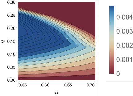
Figure 5: Maximal scaling factor $\epsilon^{*}_{\mu,q}$ as defined in Eq. (6) depending on $\mu$ and $q$. Here one allows for smaller parameters $\mu$ as in the main text, as $W_{\mu}$ becomes steerable before it becomes Bell-nonlocal. All parameter pairs yielding $\epsilon_{\mu,q}=0$ (red area) cannot be used for conclusive activation. As an inner approximation of Bob’s Bloch sphere, we have used a icosidodecahedron which has 30 vertices.

The possibility of choosing a smaller $\mu$ yields the existence if larger confidence polytopes in the sense of Eq. (6) and thus a smaller number of samples to achieve a predefined confidence level. After the filter operation, instead of demonstrating the violation of CHSH inequality, one shows the violation of a so called steering inequality, i.e., one witnesses the non-existence of a LHS model for the filtered state. Motivated by the work in Ref. Saunders et al. (2010), we consider inequalities of the form

$$S_{N}=\frac{1}{M}\sum_{k=1}^{M}\langle A_{k}\sigma_{\vec{n}_{k}}^{B}\rangle\leq C_{M},$$ (10)

where $A_{k}\in\{\pm 1\}$ is a random variable describing the outcome of Alice’s measurement (still described by a black-box as in the CHSH setting) while Bob explains his outcomes quantum mechanically via the measurement of projective measurements along directions $\vec{n}_{k}\in\mathbb{R}^{3}$. Further, $C_{M}$ denotes the largest value that $S_{M}$ can take when the correlations are explained by means of a LHS model. For the Werner state $W_{\mu}$ it is known that in the limit of $M\rightarrow\infty$ there exist measurement settings for Bob such that $W_{\mu}$ is steerable iff $\mu>1/2$ Saunders et al. (2010); Wiseman et al. (2007). For the minimal case of $M=2$ measurements, $W_{\mu}$ is steerable iff $\mu\geq 1\sqrt{2}$ where Bob’s measurement directions are given by eigenvectors of $\sigma_{x}$ and $\sigma_{y}$, forming a square on the Bloch sphere. Hence in this setting we do not obtain an decrease of the allowed parameter space of $\mu$. However, if the number of measurements is increased and the directions are chosen in an appropriate manner, the value of $C_{M}$ can be lowered significantly. In fact, it is easy to show that if the state $W_{\mu}$ is prepared, the value of $S_{M}$ in Eq. (10) is given by $\mu$. If $M=6$ and the measurement directions on Bob’s side are given by the octahedron, then one has $C_{6}\approx 0.5393$. Consequently, the parameter regime can be chosen larger, i.e., one can allow $\mu\in[0.5393,1]$ which will offer the possibility for larger confidence polytopes, see Figure 5. Indeed, one finds that for $\mu\approx 0.5410$, $q\approx 0.1836$ the maximal size of the polytope is given by $\epsilon\approx 0.0048$, which turns out to be optimal for the allowed parameter region. This implies that the number of samples needed for a conclusive activation of steerability is by a factor $23$ smaller as for the activation of Bell-nonlocality explained in the main text. More generally, increasing the number of measurement directions in Eq. (10) does not lead to a significant smaller number of required samples. For example, with $M=10$ measurement directions the steerability of $W_{\mu}$ can be revealed by $S_{10}$ for $\mu\geq 0.5236$ Saunders et al. (2010), a marginal improvement compared to $C_{6}$.

Appendix C Formulation of steerability with dichotomic measurements as semidefinite program

Here we show that deciding whether a quantum state $\varrho^{AB}$ admits a local hidden state (LHS) model for dichotomic measurements from Alice to Bob can be solved asymptotically for arbitrary states $\varrho^{AB}\in B(\mathbb{C}^{d}\otimes\mathbb{C}^{2})$. This procedure relies on a reformulation of the problem as a nesting problem of two convex objects Nguyen et al. (2018, 2019). Note that for the most general case of LHS models for generalised measurements, this procedure can in principle also be applied Nguyen et al. (2018), but is practically infeasible as the dimension of the problem grows fast. In general, no efficient method is known to decide the existence of a LHS model for all generalised measurements, even for the case of small dimensions. For that reason, we limit our construction here to dichotomic measurements, and then use Lemma 1 to further construct the LHS model for all generalised measurements.

In order to determine whether a LHS model can be constructed for a quantum state $\varrho^{AB}$ with respect to dichotomic measurements, denoted LHS₂ in the main text, one defines the critical radius as

$$R(\varrho^{AB})=\max\set{t\geq 0\colon\varrho_{t}^{AB}\,\text{admits LHS}_{2}},$$ (11)

where $\varrho_{t}^{AB}=t\varrho^{AB}+(1-t)\frac{\openone^{A}}{d_{A}}\otimes\varrho^{B}$ and $\varrho^{B}=\operatorname{tr}_{A}(\varrho^{AB})$. Note that here in the definition we implicitly assumed only dichotomic measurements. It is clear that $\varrho^{AB}$ admits a LHS model if and only if $R(\varrho^{AB})\geq 1$.

Let $\mu$ be a probability measure over the set of pure states of Bob, denoted by $\mathcal{S}^{B}$. Denote by $\mathcal{K}(\mu)$ the set of all states Alice can simulate with $\mu$, which is referred to as the (simulability) capacity of $\mu$. More precisely,

$$\mathcal{K}(\mu)=\Set{\int\mathrm{d}\mu(\sigma)g(\sigma)\sigma}{g\colon\mathcal{S}^{B}\to[0,1]}.$$ (12)

Let $\mathcal{M}^{A}$ denote the set of measurement effects of Alice and denote the corresponding conditional state for $E_{A}\in\mathcal{M}^{A}$ by $\operatorname{tr}_{A}[\varrho^{AB}(E_{A}\otimes\openone_{B})]$. Then $\varrho_{t}^{AB}$ admits a LHS model with respect to dichotomic measurements if the conditional state at Bob’s side is a subset of the set of states Alice can simulate for certain $\mu$ Nguyen et al. (2018),

$$\set{\operatorname{tr}_{A}[\varrho^{AB}(E_{A}\otimes\openone_{B})]}{E_{A}\in\mathcal{M}^{A}}\subseteq\mathcal{K}(\mu).$$ (13)

The notion of simulability capacity allows us to rewrite the critical radius as

$$\begin{split}R(\varrho)=\,\,&\text{max}\,t\\ &\text{w.r.t.}\,\,t,\mu\\ &\text{s.t.}\,\,\operatorname{tr}[\varrho_{t}^{AB}E_{A}\otimes\openone_{B}]\in\mathcal{K}(\mu)\text{ for all }E_{A}\in\mathcal{M}^{A}.\end{split}$$ (14)

Notice that the nesting condition (13) can be expressed as

$$\max_{\tau\in\mathcal{K}(\mu)}\langle Z^{B},\tau\rangle\geq\max_{E_{A}\in\mathcal{M}^{A}}\operatorname{tr}(\varrho_{t}^{AB}E_{A}\otimes Z^{B})$$ (15)

for all hermitian operators $Z^{B}$ and with $\braket{Z^{B},\tau}=\operatorname{tr}(Z^{B}\tau)$. Moreover, using the definition of $\mathcal{K}(\mu)$, one can solve the maximisation on the left hand side, which gives

$$\max_{\tau\in\mathcal{K}(\mu)}\langle Z^{B},\tau\rangle=\int\mathrm{d}\mu(\sigma)\max\{\left\langle Z^{B},\sigma\right\rangle,0\}.$$ (16)

Therefore we obtain the critical radius as

$$\begin{split}R(\varrho)=\,&\text{max}\,t\\ &\text{w.r.t.}\,\,t,\mu\\ &\text{s.t.}\,\,\int\mathrm{d}\mu(\sigma)\max\{\left\langle Z^{B},\sigma\right\rangle,0\}\geq\max_{E^{A}\in\mathcal{M}^{A}}\operatorname{tr}(\varrho_{t}^{AB}E^{A}\otimes Z^{B})\text{ for all }Z^{B}.\end{split}$$ (17)

This is an optimisation over probability measures $\mu$ supported on Bob’s Bloch sphere and with respect to an infinite number of constraints, as the whole set of hermitian operators $Z^{B}$ has to be considered. The crucial step to solve this problem is to introduce a polytope $P$ consisting of $N_{P}$ vertices, $P=\{\sigma_{i}\}_{i=1}^{N_{P}}$, approximating Bob’s Bloch sphere $S^{B}$ from inside or from outside, which gives the lower bound or upper bound of $R(\varrho^{AB})$, respectively. Upon approximating the Bloch sphere by polytope $P$, the probability measure $\mu$ turns into a probability distribution supported on the vertices. We write $u=\{p_{k}\}_{k=1}^{N_{P}}$ for this distribution, where $p_{k}=\mu(\sigma_{k})$. Correspondingly, $\mathcal{K}(\mu)$, which can be denoted by $\mathcal{K}_{P}(u)$ in this case, is also a polytope in the operator space over Bob’s system. As a consequence, in the constraints (17), one only has to consider those $Z^{B}$ corresponding to the normal vectors of the facets of $\mathcal{K}_{P}(u)$, which are of finite number. Crucially, these normal vectors of $\mathcal{K}_{P}(u)$ are only dependent on the polytope approximation $P$ of the Bloch sphere, and independent of the probability weights $u$ on the vertices of the polytope.

To find the normal vectors of the facets of the capacity $\mathcal{K}_{P}(u)$ for a polytope $P$, we follow the following reasoning. As mentioned above, for a certain operator $Z^{B}$, we have

$$\max_{\tau\in\mathcal{K}_{P}(u)}\langle Z^{B},\tau\rangle=\sum_{k=1}^{N_{P}}p_{k}\max\{\left\langle Z^{B},\sigma_{k}\right\rangle,0\}.$$ (18)

The operator $Z^{B}$ corresponds to a facet of $\mathcal{K}_{P}(u)$ if the maximisers on the left form a hyperplane in the four dimensional vector space of operators over Bob’s system. The solution on the right hand side gives the maximisers as

$$\sum_{k\in A}p_{k}\sigma_{k}+\sum_{k\in B}p_{k}\xi_{k}\sigma_{k}$$ (19)

where $A=\{k:\langle Z^{B},\sigma_{k}\rangle>0\}$ and $B=\{k:\langle Z^{B},\sigma_{k}\rangle=0\}$ with any $\xi_{k}$. One can see that this forms a hyperplane if there are at least $3$ points in $B$, that is, there are three $\sigma_{k}\in P$ such that $\langle Z^{B},\sigma_{k}\rangle=0$. This means that $P$ defines a plane that goes through at least three points of $P$. Let $\mathscr{F}(P)$ denote the set of all operator $Z^{B}$ that define a plane that goes through at least three points of $P$. Notice that $\mathscr{F}(P)$ is independent of $u$.

However, unlike the problem of two-qubit Nguyen et al. (2019), even under this polytope approximation, the problem (17) is not yet a linear program if Alice owns a qudit. Indeed, the right-hand side of the constraint in (17) still depends on $t$ in a complicated way. However, this complication can be overcome as we will explain in the following. As the objective function is linear, it follows that the maximum is attained at an extreme point of $\mathcal{M}^{A}$. The extreme points of $\mathcal{M}^{A}$ are exactly projections of rank-$l$ with $l=0,1,\ldots,d_{A}$. Consequently,

$$\max_{E^{A}\in\mathcal{M}^{A}}\operatorname{tr}(\varrho_{t}^{AB}E^{A}\otimes Z^{B})=\max_{l=0,1,\ldots,d_{A}}\max_{E^{A}\in\mathcal{M}^{A},\operatorname{tr}(E^{A})=l}\operatorname{tr}(\varrho_{t}^{AB}E^{A}\otimes Z^{B})$$ (20)

where the right-hand side indeed reduces to a linear expression of $t$,

$$t\times\max_{E^{A}\in\mathcal{M}^{A},\operatorname{tr}(E^{A})=l}\operatorname{tr}(\varrho^{AB}E^{A}\otimes Z^{B})+(1-t)l/d_{A}\operatorname{tr}(\varrho^{B}Z).$$ (21)

Hence we end up with a linear program of the form

$$\begin{split}R_{P}(\varrho^{AB})=\,&\mbox{max}\,t\\ &\text{w.r.t.}\,\,t,\{p_{k}\}_{k=1}^{N_{P}},\sum_{k=1}^{N_{P}}p_{k}=1\\ &\text{s.t.}\,\sum_{k=1}^{N_{P}}p_{k}\max\{\left\langle Z^{B},\sigma_{k}\right\rangle,0\}\geq t\eta_{l}(Z^{B})+(1-t)\frac{l}{d_{A}}\operatorname{tr}(\varrho^{B}Z^{B})\\ &\quad\text{ for all }l\text{ and for all }Z^{B}\in\mathscr{F}(P)\end{split}$$ (22)

where $\eta_{l}(Z^{B})=\max\set{\operatorname{tr}(\varrho^{AB}E^{A}\otimes Z^{B})}{E^{A}\in\mathcal{M}^{A},\operatorname{tr}(E^{A})=l}$. Notice that $\eta_{l}(Z^{B})$ is simply the sum over the $l$ maximal eigenvalues of $\operatorname{tr}_{B}(\varrho^{AB}\openone_{A}\otimes Z^{B})$.

Appendix D Construction of the confidence polytope

In quantum state tomography one measures the quantum system with a complete set of measurement settings, such that the outcome probabilities allow to identify the state. We write $E_{a|x}$ for the operator corresponding to the outcome $a$ of the measurement setting $x$. Hence, $\sum_{a}E_{a|x}=\openone$ and for projective measurements, $E_{a|x}$ is required to be a projector, while for generalised measurements it is sufficient if $E_{a|x}$ is positive semidefinite. For a system in the mixed state $\varrho$, the probability to obtain outcome $a$ in a measurement of the setting $x$ is given by

$$p_{a|x}(\varrho)=\operatorname{tr}(E_{a|x}\varrho).$$ (23)

Quantum state tomography allows us now to determine the unknown state $\varrho$ of the system. Then, for each setting $x$, one samples from the distribution $(p_{a|x}(\varrho))_{a}$, yielding after $N$ trails the relative frequencies $(f_{a|x})_{a}$. We collect all frequencies $f_{a|x}$ in a vector $\boldsymbol{f}$ and similarly for $\boldsymbol{p}(\varrho)$.

From the frequencies $\boldsymbol{f}$ one computes the free least-squares estimate, given by

$$\hat{\varrho}=\operatorname{arg\,min}_{X}\set{\lVert\boldsymbol{p}(X)-\boldsymbol{f}\rVert_{2}^{2}}{X=X^{\dagger}\text{ and }\operatorname{tr}(X)=1},$$ (24)

where the optimisation also involves matrices that are not positive semidefinite, in which case also $\boldsymbol{p}(X)$ may even become negative. Conveniently, the free least-squares estimate can be computed via $\hat{\rho}=\boldsymbol{p}^{-1}(\boldsymbol{f})$ with $\boldsymbol{p}^{-1}$ the pseudo-inverse of the linear map $X\mapsto\boldsymbol{p}(X)$. Assuming a Gaussian distribution for $\boldsymbol{f}$, one finds Eq. (3) of the main text,

$$\mathbb{P}[\,\lVert\boldsymbol{p}(\hat{\varrho})-\boldsymbol{p}(\varrho)\rVert_{2}\leq\alpha\,]\geq F_{\ell}(2N\alpha^{2}),$$ (25)

see Ref. de Almeida et al. (2023). We can rewrite this equation to

$$\mathbb{P}[\,\varrho\in\hat{\varrho}+\alpha\mathcal{E}\,]\geq F_{\ell}(2N\alpha^{2}),$$ (26)

where $\mathcal{E}=\set{Y}{\lVert\boldsymbol{p}(Y)\rVert_{2}\leq 1,\,Y=Y^{\dagger},\,\operatorname{tr}(Y)=0}$ is an ellipsoid in the set of zero-trace self-adjoint operators. Hence, the ellipsoid $\hat{\varrho}+\alpha\mathcal{E}$ constitutes a confidence region once we choose $\alpha$ according to our intended level of confidence (for example, $\gamma=99\%$), that is, we obtain $\alpha$ by solving $F_{\ell}(2N\alpha^{2})=\gamma$.

In order to obtain an outer approximation of the confidence ellipsoid in the form of a hyperoctahedron, we replace the Euclidean norm in the definition of the ellipsoid by the one-norm. For $m$ orthonormal vectors $(\boldsymbol{b}_{i})_{i}$, we use the inequality

$$\sqrt{\sum_{i}(\boldsymbol{b}_{i}\cdot\boldsymbol{v})^{2}}\geq\frac{1}{\sqrt{m}}\sum_{i}\lvert\boldsymbol{b}_{i}\cdot\boldsymbol{v}\rvert.$$ (27)

The ball $\set{\boldsymbol{v}}{\sum_{i}(\boldsymbol{b}_{i}\cdot\boldsymbol{v})^{2}\leq 1}$ is hence contained in the hyperoctahedron $\set{\sqrt{m}\,\boldsymbol{v}}{\sum_{i}\lvert\boldsymbol{b}_{i}\cdot\boldsymbol{v}\rvert\leq 1}$ with extremal points $\pm\sqrt{m}\,\boldsymbol{b}_{i}$. Since we are here interested in $\boldsymbol{v}=\boldsymbol{p}(Y)$, we need an orthonormal basis of the range of $Y\mapsto\boldsymbol{p}(Y)$ over all self-adjoint $Y$ with zero trace. This yields $\ell$ orthonormal vectors $\boldsymbol{b}_{i}=\boldsymbol{p}(Y_{i})$ with $Y_{i}$ appropriate zero-trace self-adjoint operators. After rescaling $\alpha$, we obtain Eq. (4) of the main text,

$$\mathbb{P}[\,\varrho\in\hat{\varrho}+\alpha\mathcal{P}]\geq F_{\ell}\big{(}\frac{2N}{\ell}\alpha^{2}\big{)},$$ (28)

where $\mathcal{P}$ is the hyperoctahedron spanned by $(\pm Y_{i})_{i}$. Both, the sphere and the polytope, are deformed by the linear map $\boldsymbol{p}$, see Figure 6 for an illustration.

For our specific scenario of one qutrit and one qubit we choose for the tomographic measurement the Pauli operators $\sigma_{x}$, $\sigma_{y}$, $\sigma_{z}$ for the qubit and the operators $\sigma_{0,x}$, $\sigma_{0,y}$, $\sigma_{0,z}$, $\sigma_{1,x}$, $\sigma_{1,y}$, $\sigma_{1,z}$, $\sigma_{2,x}$, $\sigma_{2,y}$ for the qutrit, where $\sigma_{i,\mu}\ket{i}=\ket{i}$ and $\sigma_{i,\mu}\ket{j}=\sigma_{\mu}\ket{j^{\prime}}$ with $j^{\prime}=j$ for $j<i$ and $j^{\prime}=j-1$ for $j>i$. We only include 3 of the 4 outcomes for each measurement setting, which yields a smaller vector $\vec{p}$ while still the above analysis is applicable. There is a freedom in the orientation of the hyperoctahedron since the operators $Y_{i}$ only need to satisfy the aforementioned orthogonality conditions. We choose the operators at random, such the orientation of the polytope does not prefer any specific direction. The specific choice of the operators $Y_{j}$ is provided in a machine-readable format upon request.

Figure 6: Illustration of the outer approximation of a confidence region by a polytope. The inner ellipsoid is the confidence region in state space. The outer polytope corresponds to the outer approximation by an octahedron.