Hadronic molecules $\eta_{c}\eta_{c}$ and $\chi_{c0}\chi_{c0}$

Abstract

The fully charmed hadronic scalar molecules $\mathcal{M}_{1}=\eta_{c}\eta_{c}$ and $\mathcal{M}_{2}=\chi_{c0}\chi_{c0}$ are studied in the context of the QCD sum rule method. The masses $m$, $\widetilde{m}$ and current couplings $f$, $\widetilde{f}$ of these states are calculated using the two-point sum rule approach. The obtained results $m=(6264\pm 50)~{}\mathrm{MeV}$ and $\widetilde{m}=(6954\pm 50)~{}\mathrm{MeV}$ are employed to determine their decay channels. It is demonstrated that the processes $\mathcal{M}_{1}\to J/\psi J/\psi$ and $\mathcal{M}_{1}\to\eta_{c}\eta_{c}$ are kinematically allowed decay modes of $\mathcal{M}_{1}$. The molecule $\mathcal{M}_{2}$ decays to $J/\psi J/\psi$, $J/\psi\psi^{\prime}$, $\eta_{c}\eta_{c}$, $\eta_{c}\eta_{c}(2S)$, $\eta_{c}\chi_{c1}(1P)$, and $\chi_{c0}\chi_{c0}$ mesons. The partial widths all of these processes are evaluated by means of the three-point sum rule calculations, which are necessary to extract the strong couplings $g_{i}$ at vertices $\mathcal{M}_{1}J/\psi J/\psi$, $\mathcal{M}_{1}\eta_{c}\eta_{c}$, and others. Our estimates for the full widths of the molecules $\Gamma_{\mathcal{M}_{1}}=(320\pm 72)~{}\mathrm{MeV}$ and $\Gamma_{\mathcal{M}_{2}}=(138\pm 18)~{}\mathrm{MeV}$, as well as their masses are compared with parameters of the $X$ resonances discovered by the LHCb-ATLAS-CMS Collaborations in the di-$J/\psi$ and $J/\psi\psi^{\prime}$ invariant mass distributions. We argue that the molecule $\mathcal{M}_{1}$ can be considered as a real candidate to the resonance $X(6200)$. The structure $\mathcal{M}_{2}$ may be interpreted as $X(6900)$ or one of its components in combination with a scalar tetraquark.

I Introduction

The discovery of the resonances $X(6200)$, $X(6600)$, $X(6900)$, and $X(7300)$ in the di-$J/\psi$ and $J/\psi\psi^{\prime}$ invariant mass distributions by the LHCb, ATLAS, and CMS Collaborations gave new impetus to investigations of fully charmed and beauty four-quark mesons LHCb:2020bwg ; Bouhova-Thacker:2022vnt ; CMS:2023owd . Heavy exotic mesons composed of two or four $c$ and $b$ quarks attracted interest of researches already at early stages of multiquark hadrons’ physics Iwasaki:1975pv ; Chao:1980dv ; Ader:1981db ; Lipkin:1986dw ; Zouzou:1986qh ; Heller:1985cb ; Carlson:1987hh ; Barnea:2006sd ; Vijande:2007ix ; Ebert:2007rn . These investigations were continued in more recent papers Berezhnoy:2011xn ; Chen:2016jxd ; Wu:2016vtq ; Bai:2016int ; Wang:2017jtz ; Debastiani:2017msn ; Richard:2017vry ; Anwar:2017toa ; Richard:2018yrm ; Esposito:2018cwh ; Liu:2019zuc ; Bedolla:2019zwg .

One of main problems studied in pioneering articles was stability of such hadrons against strong decays. It was argued that tetraquarks containing a heavy diquark and a light antidiquark may be strong-interaction stable particles, whereas fully heavy structures are unstable against strong decays (see, for instance, Refs. Ader:1981db ; Lipkin:1986dw ; Zouzou:1986qh ; Carlson:1987hh ). Detailed quantitative explorations led to different conclusions concerning allowed decay channels of fully charmed or beauty exotic mesons. Thus, in accordance with Ref. Berezhnoy:2011xn , the scalar and axial-vector tetraquarks $X_{\mathrm{4c}}=cc\overline{c}\overline{c}$ cannot decay to $J/\psi J/\psi$ mesons, because their masses are less than the di-$J/\psi$ threshold. Only a mass of a tensor tetraquark $X_{\mathrm{4c}}$ exceeds this limit and can be seen in the di-$J/\psi$ mass distribution. At the same time, all fully beauty structures $X_{\mathrm{4b}}$ are below $\Upsilon(1S)\Upsilon(1S)$ threshold, therefore do not transform strongly to these mesons. Tetraquarks $X_{\mathrm{4c}}$ and $X_{\mathrm{4b}}$ with different spin-parities were studied in Ref. Chen:2016jxd , in which it was demonstrated that scalar $X_{\mathrm{4c}}$ decays to $\eta_{c}\eta_{c}$, $J/\psi J/\psi$, and $\eta_{c}\chi_{c1}(1P)$ mesons, whereas $X_{\mathrm{4b}}$ is stable against strong decays to two bottomonia expect for a scalar diquark-antidiquark state $X_{\mathrm{4b}}$ built of pseudoscalar components.

Information of the LHCb Collaboration generated new publications aimed to explain origin of observed new structures, calculate their masses and explore possible decay channels Zhang:2020xtb ; Albuquerque:2020hio ; Becchi:2020mjz ; Becchi:2020uvq ; Dong:2020nwy ; Liang:2021fzr . Thus, the mass of the scalar tetraquark $X_{\mathrm{4c}}$ was estimated around $6.44-6.47~{}\mathrm{GeV}$ in the framework of QCD sum rule method Zhang:2020xtb , and the author interpreted $X_{\mathrm{4c}}$ as a part of a threshold enhancement $6.2-6.8\ \mathrm{GeV}$ seen by LHCb in nonresonant di-$J/\psi$ production. The hadronic molecule $\chi_{c0}\chi_{c0}$ or/and the diquark-antidiquark state with pseudoscalar constituents were considered as candidates to the resonance $X(6900)$ in Ref. Albuquerque:2020hio . Decay channels of the fully heavy tetraquarks to conventional leptons and mesons through $Q\overline{Q}$ annihilations were investigated in Refs. Becchi:2020mjz ; Becchi:2020uvq .

The LHCb data were analyzed in Ref. Dong:2020nwy in the context of a coupled-channel method: It was argued that in the di-$J/\psi$ system there is a near-threshold state $X(6200)$ having the spin-parities $0^{++}$ or $2^{++}$. The coupled-channel effects may also produce a pole structure, which was denoted as the resonance $X(6900)$ in Ref. Liang:2021fzr . The performed analysis helped the authors to declare also the existence of a bound state $X(6200)$, and the broad and narrow resonances $X(6680)$ and $X(7200)$, respectively.

The discoveries of the ATLAS and CMS experiments intensified analyses of new heavy $X$ resonances Wang:2022xja ; Dong:2022sef ; Faustov:2022mvs ; Niu:2022vqp ; Yu:2022lak ; Kuang:2023vac . In fact, in Ref. Wang:2022xja the $X(6200)$ was considered to be the ground-level tetraquark structure with $J^{\mathrm{PC}}=0^{++}$ or $1^{+-}$, whereas its first radial excitation was assigned as $X(6600)$. Similar interpretations were extended to the whole family of heavy $X$ structures in Ref. Dong:2022sef , where the authors suggested to consider the resonances $X(6200)-X(7300)$ as $1S$, $1P/2S$, $1D/2P$, and $2D/3P/4S$ tetraquark states. Close ideas were proposed in the context of the relativistic quark model as well Faustov:2022mvs .

It is clear, that a wide variety of alternatives to explain the experimental data makes important detailed investigations of fully heavy tetraquarks. In our article Agaev:2023wua , we calculated the masses of the scalar diquark-antidiquark states $X_{\mathrm{4c}}$ and $X_{\mathrm{4b}}$ built of axial-vector constituents, and estimated the full width of $X_{\mathrm{4c}}$. Our results for the mass $m=(6570\pm 55)~{}\mathrm{MeV}$ and width $\Gamma_{\mathrm{4c}}=(110\pm 21)~{}\mathrm{MeV}$ of the tetraquark $X_{\mathrm{4c}}$ allowed us to consider it as a candidate to the resonance $X(6600)$. Relying on their decay channels $X(6600)\rightarrow J/\psi J/\psi$ and $X(7300)\rightarrow J/\psi\psi^{\prime}$, we also supposed that $X(7300)$ may be $2S$ excitation of $X(6600)$: Here, we took into account that $\psi^{\prime}$ is $2S$ excited state of the meson $J/\psi$. We computed the mass of the fully beauty scalar state $X_{\mathrm{4b}}$ and got $m^{\prime}=(18540\pm 50)~{}\mathrm{MeV}$ which is below the $\eta_{b}\eta_{b}$ threshold. Hence $X_{\mathrm{4b}}$ cannot decay to hidden-bottom mesons, i.e., this tetraquark is observable neither in the $\eta_{b}\eta_{b}$ nor in $\Upsilon(1S)\Upsilon(1S)$ mass distributions. The break-up of $X_{\mathrm{4b}}$ to ordinary mesons proceeds through its strong decays to open-bottom mesons, or via electroweak leptonic and nonleptonic processes.

The scalar diquark-antidiquark states $T_{\mathrm{4c}}$ and $T_{\mathrm{4b}}$ with pseudoscalar components were explored in Ref. Agaev:2023gaq , in which we computed spectroscopic parameters of these tetraquarks. We interpreted the tetraquark $T_{\mathrm{4c}}$ with the mass $m=(6928\pm 50)~{}\mathrm{MeV}$ and width $\widetilde{\Gamma}_{\mathrm{4c}}=(128\pm 22)~{}\mathrm{MeV}$ as a resonance $X(6900)$. The mass and width of its beauty counterpart $T_{\mathrm{4b}}$ were found equal to $m^{\prime}=(18858\pm 50)~{}\mathrm{MeV}$ and $\widetilde{\Gamma}_{\mathrm{4b}}=(94\pm 28)~{}\mathrm{MeV}$, respectively.

In present article, we explore the hadronic molecules $\mathcal{M}_{1}=\eta_{c}\eta_{c}$ and $\mathcal{M}_{2}=\chi_{c0}\chi_{c0}$ by computing their masses and widths to confront obtained predictions with the both available experintal data and results of diquark-antidiquark model. The masses of these structures are evaluated using the QCD two-point sum rule method. To estimate their widths, we apply the three-point sum rule approach, which is required to extract strong couplings $g_{i}$ at vertices, for example, $\mathcal{M}_{1}J/\psi J/\psi$ and $\mathcal{M}_{1}\eta_{c}\eta_{c}$ in the case of $\mathcal{M}_{1}$.

This paper is structures in the following way: In Section II, we calculate the mass and current coupling of the molecule $\mathcal{M}_{1}$. We evaluate its full width using strong processes $\mathcal{M}_{1}\rightarrow J/\psi J/\psi$ and $\mathcal{M}_{1}\rightarrow\eta_{c}\eta_{c}$.  In Section III, we analyze in a detailed form spectroscopic parameters of the molecule $\mathcal{M}_{2}$. The full width of $\mathcal{M}_{2}$ is found by considering decays $\mathcal{M}_{2}\rightarrow J/\psi J/\psi$, $J/\psi\psi^{\prime}$, $\eta_{c}\eta_{c}$, $\eta_{c}\eta_{c}(2S)$, $\eta_{c}\chi_{c1}(1P)$ and $\mathcal{M}_{2}\rightarrow\chi_{c0}\chi_{c0}$. Last section is reserved for discussion of results and concluding remarks. Appendix contains the explicit expression of the heavy-quark propagator, and different correlation functions employed in the analyses.

II Mass, current coupling and width of the molecule $\eta_{c}\eta_{c}$

In this section, we compute the mass $m$, current coupling $f$ and full width $\Gamma_{\mathcal{M}_{1}}$ of the hadronic molecule $\mathcal{M}_{1}=\eta_{c}\eta_{c}$ using the QCD sum rule method Shifman:1978bx ; Shifman:1978by .

II.1 Mass and coupling

To derive the two-point sum rules for the mass $m$ and current coupling $f$ of the molecule $\mathcal{M}_{1}$, we explore the two-point correlation function

$$\Pi(p)=i\int d^{4}xe^{ipx}\langle 0|\mathcal{T}\{J(x)J^{{\dagger}}(0)\}|0\rangle,$$ (1)

where, $\mathcal{T}$ is the time-ordered product of two currents, and $J(x)$ is the interpolating current for the molecule $\mathcal{M}_{1}$.

The current for $\mathcal{M}_{1}$ reads

$$J(x)=\overline{c}_{a}(x)i\gamma_{5}c_{a}(x)\overline{c}_{b}(x)i\gamma_{5}c_{b}(x),$$ (2)

where $a$, and $b$ are color indices. It describes a hadronic molecule with spin-parities $J^{\mathrm{PC}}=0^{++}$.

The physical side of the sum rule $\Pi^{\mathrm{Phys}}(p)$ can be obtained from Eq. (1) by inserting a complete set of intermediate states with quark content and spin-parities of the molecule $\mathcal{M}_{1}$, and carrying out integration over $x$

$$\Pi^{\mathrm{Phys}}(p)=\frac{\langle 0|J|\mathcal{M}_{1}(p)\rangle\langle\mathcal{M}_{1}(p)|J^{\dagger}|0\rangle}{m^{2}-p^{2}}+\cdots.$$ (3)

In Eq. (3) the ground-state contribution is presented explicitly, whereas higher resonances and continuum terms are denoted by the ellipses.

The function $\Pi^{\mathrm{Phys}}(p)$ can be rewritten using the matrix element of the molecule $\mathcal{M}_{1}$

$$\langle 0|J|\mathcal{M}_{1}(p)\rangle=fm,$$ (4)

which leads to the following expression

$$\Pi^{\mathrm{Phys}}(p)=\frac{f^{2}m^{2}}{m^{2}-p^{2}}+\cdots.$$ (5)

The correlator $\Pi^{\mathrm{Phys}}(p)$ has a Lorentz structure which is proportional to $\mathrm{I}$. Consequently, corresponding invariant amplitude $\Pi^{\mathrm{Phys}}(p^{2})$ is equal to the expression in right-hand side of Eq. (5).

The second component of the sum rule analysis, i.e., the function $\Pi^{\mathrm{OPE}}(p)$ should be calculated in the operator product expansion ($\mathrm{OPE}$) with some accuracy. In terms of the $c$-quark propagators $S_{c}(x)$ the function $\Pi^{\mathrm{OPE}}(p)$ has the following form

$$\Pi^{\mathrm{OPE}}(p)=i\int d^{4}xe^{ipx}\left\{\mathrm{Tr}\left[\gamma_{5}S_{c}^{ba^{\prime}}(x)\gamma_{5}S_{c}^{a^{\prime}b}(-x)\right]\mathrm{Tr}\left[\gamma_{5}S_{c}^{ab^{\prime}}(x)\gamma_{5}S_{c}^{b^{\prime}a}(-x)\right]\right.$$

$$-\mathrm{Tr}\left[\gamma_{5}S_{c}^{bb^{\prime}}(x)\gamma_{5}S_{c}^{b^{\prime}a}(-x)\gamma_{5}S_{c}^{aa^{\prime}}(x)\gamma_{5}S_{c}^{a^{\prime}b}(-x)\right]-\mathrm{Tr}\left[\gamma_{5}S_{c}^{ba^{\prime}}(x)\gamma_{5}S_{c}^{a^{\prime}a}(-x)\gamma_{5}\right.$$

$$\left.\left.\times S_{c}^{ab^{\prime}}(x)\gamma_{5}S_{c}^{b^{\prime}b}(-x)\right]+\mathrm{Tr}\left[\gamma_{5}S_{c}^{bb^{\prime}}(x)\gamma_{5}S_{c}^{b^{\prime}b}(-x)\right]\mathrm{Tr}\left[\gamma_{5}S_{c}^{aa^{\prime}}(x)\gamma_{5}S_{c}^{a^{\prime}a}(-x)\right]\right\}.$$ (6)

The propagator $S_{c}(x)$ contains terms which are linear and quadratic in gluon field strength. As a result, $\Pi^{\mathrm{OPE}}(p)$ does not depend on light quark or mixed quark-gluon vacuum condensates. The explicit expression of $S_{c}(x)$ can be found in Appendix (see, also Ref. Agaev:2020zad ).

The $\Pi^{\mathrm{OPE}}(p)$ has also a Lorentz structure proportional $\mathrm{I}$. We denote the corresponding invariant amplitude as $\Pi^{\mathrm{OPE}}(p^{2})$. To find a sum rule equality one has to equate the functions $\Pi^{\mathrm{Phys}}(p^{2})$ and $\Pi^{\mathrm{OPE}}(p^{2})$, apply the Borel transformation for suppressing contributions of higher resonances and continuum states, and subtract suppressed terms using the assumption about quark-hadron duality Shifman:1978bx ; Shifman:1978by . After these manipulations the amplitude $\Pi^{\mathrm{OPE}}(p^{2})$ becomes a function of the Borel and continuum subtraction parameters $M^{2}$ and $s_{0}$, and will be denoted by $\Pi(M^{2},s_{0})$.

Calculation of $\Pi(M^{2},s_{0})$ is a next step to derive the sum rules for the mass $m$ and coupling $f$. Analyses demonstrate that $\Pi(M^{2},s_{0})$ has the form

$$\Pi(M^{2},s_{0})=\int_{16m_{c}^{2}}^{s_{0}}ds\rho^{\mathrm{OPE}}(s)e^{-s/M^{2}}.$$ (7)

where $\rho^{\mathrm{OPE}}(s)$ is a two-point spectral density found as an imaginary part of the invariant amplitude $\Pi^{\mathrm{OPE}}(p^{2})$. The function $\rho^{\mathrm{OPE}}(s)$ contains a perturbative term $\rho^{\mathrm{pert.}}(s)$ and a dimension-$4$ nonperturbative contribution $\sim\langle\alpha_{s}G^{2}/\pi\rangle$. An analytical expression of $\rho^{\mathrm{OPE}}(s)$ is rather cumbersome, therefore we do not write it here explicitly.

The mass $m$ and coupling $f$ can be extracted from the sum rules

$$m^{2}=\frac{\Pi^{\prime}(M^{2},s_{0})}{\Pi(M^{2},s_{0})}$$ (8)

and

$$f^{2}=\frac{e^{m^{2}/M^{2}}}{m^{2}}\Pi(M^{2},s_{0}),$$ (9)

respectively. In Eq. (8), we introduce a notation $\Pi^{\prime}(M^{2},s_{0})=d\Pi(M^{2},s_{0})/d(-1/M^{2})$.

The parameters which enter to these sum rules are the gluon vacuum condensate $\langle\alpha_{s}G^{2}/\pi\rangle$ and the mass of $c$ quark. Their numerical values are presented below

$$\langle\frac{\alpha_{s}G^{2}}{\pi}\rangle=(0.012\pm 0.004)~{}\mathrm{GeV}^{4},\ m_{c}=(1.27\pm 0.02)~{}\mathrm{GeV}.$$ (10)

A choice of the working regions for $M^{2}$ and $s_{0}$ is another problem of sum rule analyses. These parameters should be determined in such a way that to satisfy the requirement imposed by the pole contribution ($\mathrm{PC}$), and ensure convergence of the operator product expansion. Prevalence of a perturbative contribution over a nonperturbative one, as well as stability of physical quantities under variation of these parameters are also among important constraints.

Because, in the present article we consider a nonperturbative term $\sim\langle\alpha_{s}G^{2}/\pi\rangle$, the pole contribution plays a key role in determination of the working intervals for the $M^{2}$ and $s_{0}$. To estimate $\mathrm{PC}$, we use the formula

$$\mathrm{PC}=\frac{\Pi(M^{2},s_{0})}{\Pi(M^{2},\infty)},$$ (11)

and require fulfillment of the constraint $\mathrm{PC}\geq 0.5$.

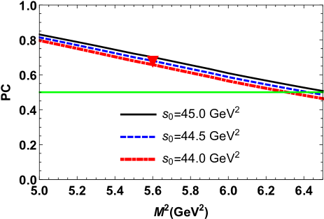
Figure 1: The pole contribution $\mathrm{PC}$ as a function of the Borel parameter $M^{2}$ at different $s_{0}$. The limit $\mathrm{PC}=0.5$ is plotted by the horizontal line. The red triangle shows the point, where the mass $m$ of $\mathcal{M}_{1}$ has effectively been extracted from the sum rule.

The $\mathrm{PC}$ is employed to fix the higher limit of the Borel parameter $M^{2}$. The lower limit for $M^{2}$, in the case under discussion, is found from a stability of the sum rules’ results under variation of $M^{2}$, and from superiority of the perturbative term. Two values of $M^{2}$ extracted by this way fix boundaries of the region where $M^{2}$ can be varied.

Calculations for the molecule $\mathcal{M}_{1}$ prove that intervals

$$M^{2}\in[5,6.5]~{}\mathrm{GeV}^{2},\ s_{0}\in[44,45]~{}\mathrm{GeV}^{2},$$ (12)

are suitable regions for the parameters $M^{2}$ and $s_{0}$, where they comply with limits on $\mathrm{PC}$ and nonperturbative term. Thus, at $M^{2}=6.5~{}\mathrm{GeV}^{2}$ the pole contribution is $0.49$, whereas at $M^{2}=5~{}\mathrm{GeV}^{2}$ it becomes equal to $0.81$. At the minimum of $M^{2}=5~{}\mathrm{GeV}^{2}$, contribution of the nonperturbative term forms $\simeq 5\%$ of the correlation function. In Fig. 1, we plot $\mathrm{PC}$ as a function of $M^{2}$ at different $s_{0}$ to show its changes in explored range of $\ M^{2}$. It is clear, that the pole contribution overshoots $0.5$ for all values of the parameters $M^{2}$ and $s_{0}$ from Eq. (12) excluding very small region around of the point $M^{2}=6.5~{}\mathrm{GeV}^{2}$.

The mass $m$ and coupling $f$ of the molecule $\mathcal{M}_{1}$ are determined by calculating them at different $M^{2}$ and $s_{0}$ from the regions Eq. (12), and averaging obtained results to find mean values of these parameters. Final results for $m$ and $f$ are

$$m=(6264\pm 50)~{}\mathrm{MeV},\ \ f=(2.12\pm 0.16)\times 10^{-2}~{}\mathrm{GeV}^{4}.$$ (13)

The predictions Eq. (13) correspond to sum rules’ results at the point $M^{2}=5.6~{}\mathrm{GeV}^{2}$ and $s_{0}=44.5~{}\mathrm{GeV}^{2}$ which is approximately at a middle of the regions Eq. (12). At this point the pole contribution is $\mathrm{PC}\approx 0.68$ which ensures superiority of $\mathrm{PC}$ in the results, and confirms ground-level nature of the molecule $\mathcal{M}_{1}$. Dependence of $m$ on the parameters $M^{2}$ and $s_{0}$ is plotted in Fig. 2.

Our result for $m$ nicely agrees with the mass of the resonance $X(6200)$

$$m^{\mathrm{ATL}}=6220\pm 50_{-50}^{+40}~{}\mathrm{MeV},$$ (14)

reported by the ATLAS Collaboration Bouhova-Thacker:2022vnt . But for reliable conclusions on a nature of the resonance $X(6200)$ there is a necessity also to estimate the full width of the molecule $\mathcal{M}_{1}$: Below, we provide results of relevant studies.

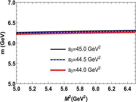
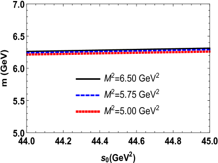
Figure 2: Mass of the hadronic molecule $\mathcal{M}_{1}$ as a function of the Borel $M^{2}$ (left), and the continuum threshold $s_{0}$ parameters (right).

II.2 Full width

The mass of the hadronic molecule $\mathcal{M}_{1}$ exceeds the two-meson $J/\psi J/\psi$ and $\eta_{c}\eta_{c}$ thresholds $6192~{}\mathrm{MeV}$ and $5968~{}\mathrm{MeV}$, respectively. Hence $S$-wave decay channels $\mathcal{M}_{1}\rightarrow J/\psi J/\psi$ and $\mathcal{M}_{1}\rightarrow\eta_{c}\eta_{c}$ are allowed modes of this particle.

II.2.1 Decay $\mathcal{M}_{1}\rightarrow J/\psi J/\psi$

We start our studies from consideration of the decay $\mathcal{M}_{1}\rightarrow J/\psi J/\psi$. Partial width of this process is determined by the strong coupling $g_{1}$ at the vertex $\mathcal{M}_{1}J/\psi J/\psi$. In the framework of the QCD sum rule method $g_{1}$ can be obtained from analysis of the three-point correlation function

$$\Pi_{\mu\nu}(p,p^{\prime})=i^{2}\int d^{4}xd^{4}ye^{ip^{\prime}y}e^{-ipx}\langle 0|\mathcal{T}\{J_{\mu}^{\psi}(y)J_{\nu}^{\psi}(0)J^{\dagger}(x)\}|0\rangle,$$ (15)

where $J_{\mu}^{\psi}(x)$ is the interpolating currents for the vector meson $J/\psi$

$$J_{\mu}^{\psi}(x)=\overline{c}_{i}(x)\gamma_{\mu}c_{i}(x),$$ (16)

where $i=1,2,3$ are the color indices. The $4$-momentum of the molecule $\mathcal{M}_{1}$ is $p$, whereas momenta of the $J/\psi$ mesons are $p^{\prime}$ and $q=p-p^{\prime}$, respectively.

After some calculations, for the physical side of the sum rule, we find

$$\Pi_{\mu\nu}^{\mathrm{Phys}}(p,p^{\prime})=g_{1}(q^{2})\frac{fmf_{1}^{2}m_{1}^{2}}{\left(p^{2}-m^{2}\right)\left(p^{\prime 2}-m_{1}^{2}\right)(q^{2}-m_{1}^{2})}$$

$$\times\left[\frac{1}{2}\left(m^{2}-m_{1}^{2}-q^{2}\right)g_{\mu\nu}-q_{\mu}p_{\nu}^{\prime}\right]+\cdots,$$ (17)

where $m_{1}$ and $f_{1}$ are the mass and decay constant of the $J/\psi$ meson. To derive Eq. (17), we have isolated the contribution of the ground-state particles from other terms, and made use the following matrix elements

$$\langle 0|J_{\mu}^{\psi}|J/\psi(p)\rangle=f_{1}m_{1}\varepsilon_{\mu}(p),$$ (18)

and

$$\langle J/\psi(p^{\prime})J/\psi(q)|\mathcal{M}_{1}(p)\rangle=g_{1}(q^{2})\left[q\cdot p^{\prime}\varepsilon^{\ast}(p^{\prime})\cdot\varepsilon^{\ast}(q)-q\cdot\varepsilon^{\ast}(p^{\prime})p^{\prime}\cdot\varepsilon^{\ast}(q)\right].$$ (19)

The correlator $\Pi_{\mu\nu}^{\mathrm{Phys}}(p,p^{\prime})$ contains two Lorentz structures that can be used to obtain the sum rule for $g_{1}(q^{2})$. We select to work with the term $\sim g_{\mu\nu}$ and present the relevant invariant amplitude by $\Pi^{\mathrm{Phys}}(p^{2},p^{\prime 2},q^{2})$. The Borel transformations over $p^{2}$ and $p^{\prime 2}$ of the amplitude $\Pi^{\mathrm{Phys}}(p^{2},p^{\prime 2},q^{2})$ yield

$$\mathcal{B}\Pi^{\mathrm{Phys}}(p^{2},p^{\prime 2},q^{2})=g_{1}(q^{2})fmf_{1}^{2}m_{1}^{2}\frac{m^{2}-m_{1}^{2}-q^{2}}{2(q^{2}-m_{1}^{2})}e^{-m^{2}/M_{1}^{2}}e^{-m_{1}^{2}/M_{2}^{2}}+\cdots.$$ (20)

The correlation function $\Pi_{\mu\nu}(p,p^{\prime})$ calculated in terms of $c$-quark propagators reads

$$\Pi_{\mu\nu}^{\mathrm{OPE}}(p,p^{\prime})=-2\int d^{4}xd^{4}ye^{ip^{\prime}y}e^{-ipx}\mathrm{Tr}\left[\gamma_{\mu}S_{c}^{ib}(y-x)\right.$$

$$\left.\times\gamma_{5}S_{c}^{bj}(x){}\gamma_{\nu}S_{c}^{ja}(-x)\gamma_{5}S_{c}^{ai}(x-y)\right].$$ (21)

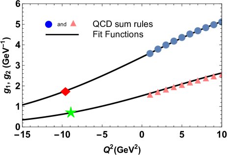
Figure 3: The sum rule predictions and fit functions for the strong couplings $g_{1}(Q^{2})$ (upper line) and $g_{2}(Q^{2})$ (lower line). The red diamond and green star denote the points $Q^{2}=-m_{1}^{2}$ and $Q^{2}=-m_{2}^{2}$, respectively.

Parameters	Values (in $\mathrm{MeV}$)
$m_{1}[m_{J/\psi}]$	$3096.900\pm 0.006$
$f_{1}[f_{J/\psi}]$	$409\pm 15$
$m_{1}^{\ast}[m_{\psi^{\prime}}]$	$3686.10\pm 0.06$
$f_{1}^{\ast}[f_{\psi^{\prime}}]$	$279\pm 8$
$m_{2}[m_{\eta_{c}}]$	$2983.9\pm 0.4$
$f_{2}[f_{\eta_{c}}]$	$398.1\pm 1.0$
$m_{2}^{\ast}[m_{\eta_{c}(2S)}]$	$3637.5\pm 1.1$
$f_{2}^{\ast}[f_{\eta_{c}(2S)}]$	$331$
$m_{3}[m_{\chi_{c1}}]$	$3510.67\pm 0.05$
$f_{3}[f_{\chi_{c1}}]$	$344\pm 27$
$m_{4}[m_{\chi_{c0}}]$	$3414.71\pm 0.30$
$f_{4}[f_{\chi_{c0}}]$	$343$

Table 1: Masses and decay constants of the various $\overline{c}c$ mesons which have been used in numerical computations.

The invariant amplitude $\Pi^{\mathrm{OPE}}(p^{2},p^{\prime 2},q^{2})$ which corresponds to the term $\sim g_{\mu\nu}$ in Eq. (21) forms the QCD side of the sum rule. Having equated the amplitudes $\Pi^{\mathrm{OPE}}(p^{2},p^{\prime 2},q^{2})$ and $\Pi^{\mathrm{Phys}}(p^{2},p^{\prime 2},q^{2})$ and performed the doubly Borel transforms and continuum subtractions, one can find the sum rule for the form factor $g_{1}(q^{2})$

$$g_{1}(q^{2})=\frac{2}{fmf_{1}^{2}m_{1}^{2}}\frac{q^{2}-m_{1}^{2}}{m^{2}-m_{1}^{2}-q^{2}}e^{m^{2}/M_{1}^{2}}e^{m_{1}^{2}/M_{2}^{2}}\Pi(\mathbf{M}^{2},\mathbf{s}_{0},q^{2}).$$ (22)

Here,

$$\Pi(\mathbf{M}^{2},\mathbf{s}_{0},q^{2})=\int_{16m_{c}^{2}}^{s_{0}}ds\int_{4m_{c}^{2}}^{s_{0}^{\prime}}ds^{\prime}\rho(s,s^{\prime},q^{2})e^{-s/M_{1}^{2}}e^{-s^{\prime}/M_{2}^{2}},$$ (23)

is the function $\Pi^{\mathrm{OPE}}(p^{2},p^{\prime 2},q^{2})$ after the Borel transformations and subtraction procedures. It is expressed using the spectral density $\rho(s,s^{\prime},q^{2})$: the latter is calculated as a relevant imaginary part of $\Pi_{\mu\nu}^{\mathrm{OPE}}(p,p^{\prime})$. In Eq. (23) $\mathbf{M}^{2}=(M_{1}^{2},M_{2}^{2})$ and $\mathbf{s}_{0}=(s_{0},s_{0}^{\prime})$ are the Borel and continuum threshold parameters, respectively.

The form factor $g_{1}(q^{2})$ depends on the masses and decay constants of the molecule $\mathcal{M}_{1}$ and meson $J/\psi$ , which are input parameters in calculations. Their numerical values are collected in Table 1. Additionally, this table contains the parameters of the $\psi^{\prime}$, $\eta_{c}$, $\eta_{c}(2S)$, $\chi_{c1}(1P)$, and $\chi_{c0}(1P)$ mesons which are necessary to explore decay modes of the hadronic molecules $\mathcal{M}_{1}$ and $\mathcal{M}_{2}$. For the masses of the particles, we utilize information from Ref. PDG:2022 . For decay constant of the meson $J/\psi$, we employ the experimental value from Ref. Kiselev:2001xa . As $f_{\eta_{c}}$ we use results of the QCD lattice simulations Hatton:2020qhk , whereas for $f_{\chi_{c1}}$ and $f_{\chi_{c0}}$ – the sum rule predictions from Refs. VeliVeliev:2012cc ; Veliev:2010gb .

To carry out numerical computations, it is also necessary to choose the working regions for the parameters $\mathbf{M}^{2}$ and $\mathbf{s}_{0}$. For $M_{1}^{2}$ and $s_{0}$, associated with the $\mathcal{M}_{1}$ channel, we apply the working windows of Eq. (12). The parameters $(M_{2}^{2},\ s_{0}^{\prime})$ for the $J/\psi$ channel are varied inside the intervals

$$M_{2}^{2}\in[4,5]~{}\mathrm{GeV}^{2},\ s_{0}^{\prime}\in[12,13]~{}\mathrm{GeV}^{2}.$$ (24)

It is a fact that the sum rule approach leads to reliable predictions in the deep-Euclidean region $q^{2}<0$. For our purposes, it is suitable to introduce a new variable $Q^{2}=-q^{2}$ and present the obtained function by $g_{1}(Q^{2})$. The interval of $Q^{2}$ studied by the sum rule analysis contains the region $Q^{2}=1-10~{}\mathrm{GeV}^{2}$. The results of analyses are plotted in Fig. 3.

But the width of the decay $\mathcal{M}_{1}\rightarrow J/\psi J/\psi$ is determined by the the form factor $g_{1}(q^{2})$ at the mass shell $q^{2}=m_{1}^{2}$, i.e., one has to find $g_{1}(Q^{2}=-m_{1}^{2})$. To overcome this problem, we use a fit function $\mathcal{G}_{1}(Q^{2})$, which at momenta $Q^{2}>0$ gives the same values as the sum rule predictions, but it can be extrapolated to the region of $Q^{2}<0$. In this paper, we employ the functions $\mathcal{G}_{i}(Q^{2})$

$$\mathcal{G}_{i}(Q^{2})=\mathcal{G}_{i}^{0}\mathrm{\exp}\left[c_{i}^{1}\frac{Q^{2}}{m^{2}}+c_{i}^{2}\left(\frac{Q^{2}}{m^{2}}\right)^{2}\right]$$ (25)

with parameters $\mathcal{G}_{i}^{0}$, $c_{i}^{1}$, and $c_{i}^{2}$.

Calculations demonstrate that $\mathcal{G}_{1}^{0}=3.41~{}\mathrm{GeV}^{-1}$, $c_{1}^{1}=2.18$, and $c_{1}^{2}=-2.21$ lead to reasonable agreement with the sum rule’s data for $g_{1}(Q^{2})$ depicted in Fig. 3. At the mass shell $q^{2}=m_{1}^{2}$ the function $\mathcal{G}_{1}(Q^{2})$ equals to

$$g_{1}\equiv\mathcal{G}_{1}(-m_{1}^{2})=(1.75\pm 0.41)\ \mathrm{GeV}^{-1}.$$ (26)

The partial width of the process $\mathcal{M}_{1}\rightarrow J/\psi J/\psi$ can be obtained by means of the following formula

$$\Gamma\left[\mathcal{M}_{1}\rightarrow J/\psi J/\psi\right]=g_{1}^{2}\frac{\lambda_{1}}{8\pi}\left(\frac{m_{1}^{4}}{m^{2}}+\frac{2\lambda_{1}^{2}}{3}\right),$$ (27)

where $\lambda_{1}=\lambda(m,m_{1},m_{1})$ and

$$\lambda(a,b,c)=\frac{\sqrt{a^{4}+b^{4}+c^{4}-2(a^{2}b^{2}+a^{2}c^{2}+b^{2}c^{2})}}{2a}.$$ (28)

It is easy to find that

$$\Gamma\left[\mathcal{M}_{1}\rightarrow J/\psi J/\psi\right]=(142\pm 47)~{}\mathrm{MeV}.$$ (29)

II.2.2 Process $\mathcal{M}_{1}\rightarrow\eta_{c}\eta_{c}$

The process $\mathcal{M}_{1}\rightarrow\eta_{c}\eta_{c}$ is another decay channel of the hadronic molecule $\mathcal{M}_{1}$. Investigation of this process runs, with some modifications, in accordance with the scheme explained above. The strong coupling $g_{2}$ that describes the vertex $\mathcal{M}_{1}\eta_{c}\eta_{c}$ is extracted from the correlation function

$$\Pi(p,p^{\prime})=i^{2}\int d^{4}xd^{4}ye^{ip^{\prime}y}e^{-ipx}\langle 0|\mathcal{T}\{J^{\eta_{c}}(y)J^{\eta_{c}}(0)J^{\dagger}(x)\}|0\rangle,$$ (30)

where

$$J^{\eta_{c}}(x)=\overline{c}_{i}(x)i\gamma_{5}c_{i}(x),$$ (31)

is the interpolating current for the meson $\eta_{c}$.

The physical side of the sum rule for the form factor $g_{2}(q^{2})$ is derived by separating the contribution of the ground-state and the effects of the higher states and continuum from each other. Then, the correlation function (30) can be presented in the following form

$$\Pi^{\mathrm{Phys}}(p,p^{\prime})=\frac{\langle 0|J^{\eta_{c}}|\eta_{c}(p^{\prime})\rangle}{p^{\prime 2}-m_{2}^{2}}\frac{\langle 0|J^{\eta_{c}}|\eta_{c}(q)\rangle}{q^{2}-m_{2}^{2}}\langle\eta_{c}(p^{\prime})\eta_{c}(q)|\mathcal{M}_{1}(p)\rangle$$

$$\times\frac{\langle\mathcal{M}_{1}(p)|J^{\dagger}|0\rangle}{p^{2}-m^{2}}+\cdots,$$ (32)

with $m_{2}$ being the mass of the $\eta_{c}$ meson.

We define the vertex composed of a scalar and two pseudoscalar particles by means of the formula

$$\langle\eta_{c}(p^{\prime})\eta_{c}(q)|\mathcal{M}_{1}(p)\rangle=g_{2}(q^{2})p\cdot p^{\prime}.$$ (33)

To rewrite the correlator $\Pi^{\mathrm{Phys}}(p,p^{\prime})$ in terms of physical parameters of particles $\mathcal{M}_{1}$ and $\eta_{c}$, we also use the matrix elements Eq. (4) and

$$\langle 0|J^{\eta_{c}}|\eta_{c}\rangle=\frac{f_{2}m_{2}^{2}}{2m_{c}},$$ (34)

where $f_{2}$ is the decay constant of the $\eta_{c}$ meson. The correlation function $\Pi^{\mathrm{Phys}}(p,p^{\prime})$ then becomes equal to

$$\Pi^{\mathrm{Phys}}(p,p^{\prime})=g_{2}(q^{2})\frac{fmf_{2}^{2}m_{2}^{4}}{4m_{c}^{2}\left(p^{2}-m^{2}\right)\left(p^{\prime 2}-m_{2}^{2}\right)}\frac{m^{2}+m_{2}^{2}-q^{2}}{2(q^{2}-m_{2}^{2})}+\cdots.$$ (35)

The function $\Pi^{\mathrm{Phys}}(p,p^{\prime})$ has a Lorentz structure which is proportional to $\mathrm{I}$, hence right-hand side of Eq. (35) is the corresponding invariant amplitude $\widehat{\Pi}^{\mathrm{Phys}}(p^{2},p^{\prime 2},q^{2})$.

We also find the function $\Pi^{\mathrm{OPE}}(p,p^{\prime})$

$$\Pi^{\mathrm{OPE}}(p,p^{\prime})=2i^{2}\int d^{4}xd^{4}ye^{ip^{\prime}y}e^{-ipx}\left\{\mathrm{Tr}\left[\gamma_{5}S_{c}^{ia}(y-x)\gamma_{5}S_{c}^{ai}(x-y)\right]\right.$$

$$\left.\times\mathrm{Tr}\left[\gamma_{5}S_{c}^{jb}(-x)\gamma_{5}S_{c}^{bj}(x){}\right]-\mathrm{Tr}\left[\gamma_{5}S_{c}^{ia}(y-x)\gamma_{5}S_{c}^{aj}(x){}\gamma_{5}S_{c}^{jb}(-x)\gamma_{5}S_{c}^{bi}(x-y)\right]\right\},$$ (36)

and denote the amplitude corresponding to a structure $\sim\mathrm{I}$ by $\widehat{\Pi}^{\mathrm{OPE}}(p^{2},p^{\prime 2},q^{2})$. The sum rule for the strong form factor $g_{2}(q^{2})$ reads

$$g_{2}(q^{2})=\frac{8m_{c}^{2}}{fmf_{2}^{2}m_{2}^{4}}\frac{q^{2}-m_{2}^{2}}{m^{2}+m_{2}^{2}-q^{2}}e^{m^{2}/M_{1}^{2}}e^{m_{2}^{2}/M_{2}^{2}}\widehat{\Pi}(\mathbf{M}^{2},\mathbf{s}_{0},q^{2}).$$ (37)

Numerical computations are carried out using the parameters of the meson $\eta_{c}$ from Table 1. The Borel and continuum subtraction parameters $M_{1}^{2}$ and $s_{0}$ in the $\mathcal{M}_{1}$ channel is chosen as in Eq. (12), whereas for $M_{2}^{2}$ and $s_{0}^{\prime}$ that correspond to the $\eta_{c}$ channel, we employ

$$M_{2}^{2}\in[3.5,4.5]~{}\mathrm{GeV}^{2},\ s_{0}^{\prime}\in[11,12]~{}\mathrm{GeV}^{2}.$$ (38)

The fit function $\mathcal{G}_{2}(Q^{2})$ has the following parameters: $\mathcal{G}_{2}^{0}=1.52~{}\mathrm{GeV}^{-1}$, $c_{2}^{1}=2.84$, and $c_{2}^{2}=-2.73$. For the strong coupling $g_{2}$, we get

$$g_{2}\equiv\mathcal{G}_{2}(-m_{2}^{2})=(6.9\pm 1.5)\times 10^{-1}\ \mathrm{GeV}^{-1}.$$ (39)

The width of the process $\mathcal{M}_{1}\rightarrow\eta_{c}\eta_{c}$ is determined by means of the formula

$$\Gamma\left[\mathcal{M}_{1}\rightarrow\eta_{c}\eta_{c}\right]=g_{2}^{2}\frac{m_{2}^{2}\lambda_{2}}{8\pi}\left(1+\frac{\lambda_{2}^{2}}{m_{2}^{2}}\right),$$ (40)

where $\lambda_{2}=\lambda(m,m_{2},m_{2})$. Finally, we obtain

$$\Gamma\left[\mathcal{M}_{1}\rightarrow\eta_{c}\eta_{c}\right]=(178\pm 55)~{}\mathrm{MeV}.$$ (41)

The parameters of the decays $\mathcal{M}_{1}\rightarrow J/\psi J/\psi$ and $\mathcal{M}_{1}\rightarrow\eta_{c}\eta_{c}$ are shown in Table 2.

Based on these results, it is not difficult to find that

$$\Gamma_{\mathcal{M}_{1}}=(320\pm 72)~{}\mathrm{MeV},$$ (42)

which is the full width of the hadronic molecule $\mathcal{M}_{1}$.

$i$	Channels	$g_{i}^{(\ast)}\times 10~{}(\mathrm{GeV}^{-1})$	$\Gamma_{i}~{}(\mathrm{MeV})$
$1$	$\mathcal{M}_{1}\to J/\psi J/\psi$	$17.5\pm 4.1$	$142\pm 47$
$2$	$\mathcal{M}_{1}\to\eta_{c}\eta_{c}$	$6.9\pm 1.5$	$178\pm 55$
$3$	$\mathcal{M}_{2}\to J/\psi J\psi$	$4.1\pm 0.8$	$38\pm 11$
$3^{\ast}$	$\mathcal{M}_{2}\to J/\psi\psi^{\prime}$	$3.3\pm 0.7$	$11\pm 4$
$4$	$\mathcal{M}_{2}\to\eta_{c}\eta_{c}$	$2.1\pm 0.4$	$39\pm 11$
$4^{\ast}$	$\mathcal{M}_{2}\to\eta_{c}\eta_{c}(2S)$	$1.34\pm 0.26$	$12\pm 4$
$5$	$\mathcal{M}_{2}\to\eta_{c}\chi_{c1}$	$29\pm 6^{\star}$	$16\pm 5$
$6$	$\mathcal{M}_{2}\to\chi_{c0}\chi_{c0}$	$2.7\pm 0.43$	$22\pm 5$

Table 2: Decay channels of the molecules $\mathcal{M}_{1(2)}$, strong couplings $g_{i}^{(\ast)}$, and partial widths $\Gamma_{i}$. The star-labeled coupling $g_{5}$ is dimensionless.

III Hadronic molecule $\chi_{c0}\chi_{c0}$

This part of the article is devoted to thorough investigations of the molecule $\mathcal{M}_{2}=\chi_{c0}\chi_{c0}$ which imply calculations of the mass $\widetilde{m}$ and coupling $\widetilde{f}$, as well as the full width $\Gamma_{\mathcal{M}_{2}}$ of this compound by employing its numerous decay modes.

III.1 Spectroscopic parameters $\widetilde{m}$ and $\widetilde{f}$

In the case of the molecule $\mathcal{M}_{2}=\chi_{c0}\chi_{c0}$ the two-point correlation function that should be analyzed has the form

$$\widetilde{\Pi}(p)=i\int d^{4}xe^{ipx}\langle 0|\mathcal{T}\{\widetilde{J}(x)\widetilde{J}^{{\dagger}}(0)\}|0\rangle,$$ (43)

where $\widetilde{J}(x)$ is the interpolating current for the molecule $\mathcal{M}_{2}$. We treat $\mathcal{M}_{2}$ as a hadronic state built of the scalar mesons $\chi_{c0}\chi_{c0}$, therefore define the relevant interpolating current as

$$\widetilde{J}(x)=\overline{c}_{a}(x)c_{a}(x)\overline{c}_{b}(x)c_{b}(x).$$ (44)

The physical side of the sum rule

$$\widetilde{\Pi}^{\mathrm{Phys}}(p)=\frac{\widetilde{f}^{2}\widetilde{m}^{2}}{\widetilde{m}^{2}-p^{2}}+\cdots,$$ (45)

does not differ from Eq. (5), but $\widetilde{m}$ and $\widetilde{f}$ are now the mass and coupling of the molecule $\mathcal{M}_{2}$ introduced through the matrix element

$$\langle 0|\widetilde{J}|\mathcal{M}_{2}(p)\rangle=\widetilde{f}\widetilde{m}.$$ (46)

The amplitude $\widetilde{\Pi}^{\mathrm{Phys}}(p^{2})$ required for the following analysis is given by the expression in the right-hand side of Eq. (45).

The correlation function $\widetilde{\Pi}^{\mathrm{OPE}}(p)$ computed using the $c$-quark propagators is written down in Eq. (A.85). The sum rules for $\widetilde{m}$ and $\widetilde{f}$ are determined by Eqs. (8) and (9) with evident replacements.

The working windows for the Borel and continuum subtraction parameters $M^{2}$ and $s_{0}$ are:

$$M^{2}\in[5.5,7]~{}\mathrm{GeV}^{2},\ s_{0}\in[54,55]~{}\mathrm{GeV}^{2}.$$ (47)

At $M^{2}=5.5~{}\mathrm{GeV}^{2}$ and $7~{}\mathrm{GeV}^{2}$ the pole contribution constitutes $\mathrm{PC}=0.75$ and $0.48$ parts of the correlation function, respectively. The pole contribution changes within limits

$$0.75\geq\mathrm{PC}\geq 0.48.$$ (48)

On average in $s_{0}$ the pole contribution is $\mathrm{PC}\geq 0.5$. The dimension-$4$ term is negative and at $M^{2}=5.5~{}\mathrm{GeV}^{2}$ constitutes $\simeq 19.9\%$ of the correlator.

The mass and current coupling of $\mathcal{M}_{2}$ are:

$$\widetilde{m}=(6954\pm 50)~{}\mathrm{MeV},\ \ \widetilde{f}=(1.71\pm 0.12)\times 10^{-2}~{}\mathrm{GeV}^{4}.$$ (49)

These results are obtained as mean values of $\widetilde{m}$ and $\widetilde{f}$ averaged over the regions Eq. (47). They effectively correspond to the sum rule predictions at the point $M^{2}=6.2~{}\mathrm{GeV}^{2}$ and $s_{0}=54.5~{}\mathrm{GeV}^{2}$, where $\mathrm{PC}=0.64$. In Fig. 4, we plot $\widetilde{m}$ as a function of $M^{2}$ and $s_{0}$.

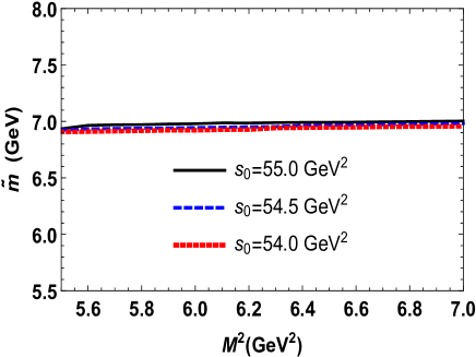
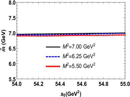
Figure 4: Dependence of the $\mathcal{M}_{2}$ molecule’s mass $\widetilde{m}$ on the parameters $M^{2}$ (left), and $s_{0}$ (right).

III.2 Decays of $\mathcal{M}_{2}$

The prediction for the mass of the molecule $\mathcal{M}_{2}$ determines its kinematically allowed decay channels. First of all, they are processes $\mathcal{M}_{2}\rightarrow J/\psi J/\psi$ and $\mathcal{M}_{2}\rightarrow J/\psi\psi^{\prime}$. The $\widetilde{m}$ satisfies kinematical restrictions for productions of $\eta_{c}\eta_{c}$ and $\eta_{c}\eta_{c}(2S)$ pairs. The $\mathcal{M}_{2}$ can decay to $\eta_{c}\chi_{c1}(1P)$ and $\chi_{c0}\chi_{c0}$ mesons as well. The decay $\mathcal{M}_{2}\rightarrow\eta_{c}\chi_{c1}(1P)$ is the $P$-wave process, whereas other ones are $S$-wave modes.

III.2.1 $\mathcal{M}_{2}\rightarrow J/\psi J/\psi$ and $\mathcal{M}_{2}\rightarrow J/\psi\psi^{\prime}$

The three-point sum rules for the strong form factors $g_{3}(q^{2})$ and $g_{3}^{\ast}(q^{2})$ which describe interaction of particles at vertices $\mathcal{M}_{2}J/\psi J/\psi$  and $\mathcal{M}_{2}J/\psi\psi^{\prime}$ respectively, can be extracted from studies of the correlation function

$$\widetilde{\Pi}_{\mu\nu}(p,p^{\prime})=i^{2}\int d^{4}xd^{4}ye^{ip^{\prime}y}e^{-ipx}\langle 0|\mathcal{T}\{J_{\mu}^{\psi}(y)J_{\nu}^{\psi}(0)\widetilde{J}^{\dagger}(x)\}|0\rangle.$$ (50)

Firstly, we express $\widetilde{\Pi}_{\mu\nu}(p,p^{\prime})$ using the physical parameters of particles involved in these decays. The molecule $\mathcal{M}_{2}$ can decay to $J/\psi J/\psi$ and $J/\psi\psi^{\prime}$ mesons, therefore in $\widetilde{\Pi}_{\mu\nu}(p,p^{\prime})$ we isolate contributions of the particles $J/\psi$ and $\psi^{\prime}$ from effects of higher resonances and continuum states. Then, the physical side of the sum rule $\widetilde{\Pi}_{\mu\nu}^{\mathrm{Phys}}(p,p^{\prime})$ is determined by Eq. (A.86). It can be rewritten using the matrix elements of the particles $\mathcal{M}_{2}$, $J/\psi$ and $\psi^{\prime}$

$$\widetilde{\Pi}_{\mu\nu}^{\mathrm{Phys}}(p,p^{\prime})=g_{3}(q^{2})\frac{\widetilde{f}\widetilde{m}f_{1}^{2}m_{1}^{2}}{\left(p^{2}-\widetilde{m}^{2}\right)\left(p^{\prime 2}-m_{1}^{2}\right)(q^{2}-m_{1}^{2})}\left[\frac{1}{2}\left(\widetilde{m}^{2}-m_{1}^{2}-q^{2}\right)g_{\mu\nu}-q_{\mu}p_{\nu}^{\prime}\right]$$

$$+g_{3}^{\ast}(q^{2})\frac{\widetilde{f}\widetilde{m}f_{1}m_{1}f_{1}^{\ast}m_{1}^{\ast}}{\left(p^{2}-\widetilde{m}^{2}\right)\left(p^{\prime 2}-m_{1}^{\ast 2}\right)(q^{2}-m_{1}^{2})}\left[\frac{1}{2}\left(\widetilde{m}^{2}-m_{1}^{\ast 2}-q^{2}\right)g_{\mu\nu}-q_{\mu}p_{\nu}^{\prime}\right]+\cdots,$$

(51)

where $m_{1}^{\ast}$ and $f_{1}^{\ast}$ are the mass and decay constant of the meson $\psi^{\prime}$. In what follows, we use the component of $\widetilde{\Pi}_{\mu\nu}^{\mathrm{Phys}}(p,p^{\prime})$ that is proportional to $g_{\mu\nu}$, and denote the relevant invariant amplitude by $\widetilde{\Pi}^{\mathrm{Phys}}(p^{2},p^{\prime 2},q^{2})$.

The second term of the sum rules,  i.e., the correlation function $\widetilde{\Pi}_{\mu\nu}^{\mathrm{OPE}}(p,p^{\prime})$ is presented in Eq. (A.87). An amplitude $\widetilde{\Pi}^{\mathrm{OPE}}(p^{2},p^{\prime 2},q^{2})$ which corresponds to the term $\sim g_{\mu\nu}$ in $\widetilde{\Pi}_{\mu\nu}^{\mathrm{OPE}}(p,p^{\prime})$ establishes the QCD side of the sum rules. By equating the amplitudes $\widetilde{\Pi}^{\mathrm{OPE}}(p^{2},p^{\prime 2},q^{2})$ and $\widetilde{\Pi}^{\mathrm{Phys}}(p^{2},p^{\prime 2},q^{2})$, applying the the Borel transformations and carrying out continuum subtractions, one can find the sum rules for the form factors $g_{3}(q^{2})$ and $g_{3}^{\ast}(q^{2})$. Let us note after these manipulations the $\widetilde{\Pi}^{\mathrm{OPE}}(p^{2},p^{\prime 2},q^{2})$ takes the form Eq. (23) with a new spectral density $\widetilde{\rho}(s,s^{\prime},q^{2})$.

To find the form factors $g_{3}(q^{2})$ and $g_{3}^{\ast}(q^{2})$, we keep the following approach. At the first phase, we compute the form factor $g_{3}(q^{2})$ by choosing in the $J/\psi$ channel $4m_{c}^{2}<s_{0}^{\prime}<m_{1}^{\ast 2}$. This means that, we exclude the second term in Eq. (51) from analysis by including it into higher resonances and continuum states. As a result, the physical side of the sum rule contains a contribution coming only from ground-level states. The sum rule for the form factor $g_{3}(q^{2})$ is determined by Eq. (22) after substitutions $\Pi(\mathbf{M}^{2},\mathbf{s}_{0},q^{2})\rightarrow\widetilde{\Pi}(\mathbf{M}^{2},\mathbf{s}_{0},q^{2})$ and $fm\rightarrow\widetilde{f}\widetilde{m}$. At the second stage of computations, we fix $s_{0}^{\ast\prime}>$ $m_{1}^{\ast 2}$, and take into account the second term in Eq. (51). Afterwards, using results obtained for $g_{3}(q^{2})$, we determine $g_{3}^{\ast}(q^{2})$.

In numerical computations the working regions for $M_{1}^{2}$ and $s_{0}$ in the $\mathcal{M}_{2}$ channel are chosen as in Eq. (47). The parameters $(M_{2}^{2},\ s_{0}^{\prime})$ for the $J/\psi$ channel are changed within limits given by Eq. (24). The sum rule calculations are carried out in deep-Euclidean region $q^{2}=-(1\div 10)~{}\mathrm{GeV}^{2}$. The fit function $\mathcal{G}_{3}(Q^{2})$ necessary to extrapolate these data to region of $q^{2}>0$ has the parameters $\mathcal{G}_{3}^{0}=0.87~{}\mathrm{GeV}^{-1}$, $c_{3}^{1}=3.03$, and $c_{3}^{2}=-3.64$. At the mass shell $q^{2}=m_{1}^{2}$ this function determines the strong coupling $g_{3}$

$$g_{3}\equiv\mathcal{G}_{3}(-m_{1}^{2})=(4.1\pm 0.8)\times 10^{-1}\ \mathrm{GeV}^{-1}.$$ (52)

Partial width of the process $\mathcal{M}_{2}\rightarrow J/\psi J/\psi$ can be found by means of Eq. (27) after substitutions $g_{1}\rightarrow g_{3}$, $m^{2}\rightarrow\widetilde{m}^{2}$ and $\lambda_{1}\rightarrow\lambda_{3}=\lambda(\widetilde{m},m_{1},m_{1})$. It is not difficult to get

$$\Gamma\left[\mathcal{M}_{2}\rightarrow J/\psi J/\psi\right]=(38\pm 11)~{}\mathrm{MeV}.$$ (53)

The process $\mathcal{M}_{2}\rightarrow J/\psi\psi^{\prime}$ can be studied in accordance with a scheme described above. In this phase of the analysis, in the $\psi^{\prime}$ channel, we employ

$$M_{2}^{2}\in[4,5]~{}\mathrm{GeV}^{2},\ s_{0}^{\ast\prime}\in[15,16]~{}\mathrm{GeV}^{2}.$$ (54)

It is worth noting that $s_{0}^{\ast\prime}$ is limited by the mass $m(3S)=4039~{}\mathrm{MeV}$ of the charmonium $\psi(3S)$ PDG:2022 . For this decay, the extrapolating function $\mathcal{G}_{3}^{\ast}(Q^{2})$ has the parameters $\mathcal{G}_{3}^{0\ast}=0.68~{}\mathrm{GeV}^{-1}$, $c_{3}^{1\ast}=2.90$, and $c_{3}^{2\ast}=-3.54$. The strong coupling $g_{3}^{\ast}$ is calculated at the mass shell $q^{2}=m_{1}^{2}$

$$g_{3}^{\ast}\equiv\mathcal{G}_{3}^{\ast}(-m_{1}^{2})=(3.3\pm 0.7)\times 10^{-1}\ \mathrm{GeV}^{-1}.$$ (55)

The partial width of the decay $\mathcal{M}_{2}\rightarrow J/\psi\psi^{\prime}$ is

$$\Gamma\left[\mathcal{M}_{2}\rightarrow J/\psi\psi^{\prime}\right]=(11\pm 4)~{}\mathrm{MeV}.$$ (56)

III.2.2 $\mathcal{M}_{2}\rightarrow\eta_{c}\eta_{c}$ and $\mathcal{M}_{2}\rightarrow\eta_{c}\eta_{c}(2S)$

The processes $\mathcal{M}_{2}\rightarrow\eta_{c}\eta_{c}$ and $\mathcal{M}_{2}\rightarrow\eta_{c}\eta_{c}(2S)$ can be investigated by the similar manner. The strong couplings $g_{4}$ and $g_{4}^{\ast}$ that correspond to the vertices $\mathcal{M}_{2}\eta_{c}\eta_{c}$ and $\mathcal{M}_{2}\eta_{c}\eta_{c}(2S)$ can be extracted from the correlation function

$$\widetilde{\Pi}(p,p^{\prime})=i^{2}\int d^{4}xd^{4}ye^{ip^{\prime}y}e^{-ipx}\langle 0|\mathcal{T}\{J^{\eta_{c}}(y)J^{\eta_{c}}(0)\widetilde{J}^{\dagger}(x)\}|0\rangle.$$ (57)

Separating the ground-level and first excited state contributions from effects of higher resonances and continuum states, we can write the correlation function $\widetilde{\Pi}^{\mathrm{Phys}}(p,p^{\prime})$ which is determined by Eq. (A.88). It can be further simplified using known matrix elements and takes the form

$$\widetilde{\Pi}^{\mathrm{Phys}}(p,p^{\prime})=g_{4}(q^{2})\frac{\widetilde{f}\widetilde{m}f_{2}^{2}m_{2}^{4}}{8m_{c}^{2}\left(p^{2}-\widetilde{m}^{2}\right)\left(p^{\prime 2}-m_{2}^{2}\right)}\frac{\widetilde{m}^{2}+m_{2}^{2}-q^{2}}{q^{2}-m_{2}^{2}}$$

$$+g_{4}^{\ast}(q^{2})\frac{\widetilde{f}\widetilde{m}f_{2}m_{2}^{2}f_{2}^{\ast}m_{2}^{\ast 2}}{8m_{c}^{2}\left(p^{2}-\widetilde{m}^{2}\right)\left(p^{\prime 2}-m_{2}^{\ast 2}\right)}\frac{\widetilde{m}^{2}+m_{2}^{\ast 2}-q^{2}}{q^{2}-m_{2}^{2}}+\cdots.$$ (58)

where $m_{2}^{\ast}$ and $f_{2}^{\ast}$ are the mass and decay constant of the $\eta_{c}(2S)$ meson. The correlation function $\widetilde{\Pi}^{\mathrm{Phys}}(p,p^{\prime})$ has simple Lorentz structure proportional to $\mathrm{I}$, hence right-hand side of Eq. (58) is the corresponding invariant amplitude $\widetilde{\Pi}^{\mathrm{Phys}}(p^{2},p^{\prime 2},q^{2})$.

The QCD side of the sum rule $\widetilde{\Pi}^{\mathrm{OPE}}(p,p^{\prime})$ is given by Eq. (A.89). The sum rule for the strong form factor $g_{4}(q^{2})$ is determined by Eq. (37) with replacements $fm\rightarrow\widetilde{f}\widetilde{m}$ and $\widehat{\Pi}\rightarrow\widetilde{\Pi}$, where $\widetilde{\Pi}(\mathbf{M}^{2},\mathbf{s}_{0},q^{2})$ corresponds to the correlation function $\widetilde{\Pi}^{\mathrm{OPE}}(p,p^{\prime})$.

Numerical computations are carried out using Eq. (37), parameters of the meson $\eta_{c}$ from Table 1, and working regions for $\mathbf{M}^{2}$ and $\mathbf{s}_{0}$. The Borel and continuum subtraction parameters $M_{1}^{2}$ and $s_{0}$ in the $\mathcal{M}_{2}$ channel are chosen as in Eq. (47), whereas for $M_{2}^{2}$ and $s_{0}^{\prime}$ which correspond to the $\eta_{c}$ channel, we employ Eq. (38).

The interpolating function $\mathcal{G}_{4}(Q^{2})$ necessary to determine the coupling $g_{4}$ has the parameters: $\mathcal{G}_{4}^{0}=0.48~{}\mathrm{GeV}^{-1}$, $c_{4}^{1}=3.65$, and $c_{4}^{2}=-4.24$. For the strong coupling $g_{4}$, we get

$$g_{4}\equiv\mathcal{G}_{4}(-m_{2}^{2})=(2.1\pm 0.4)\times 10^{-1}\ \mathrm{GeV}^{-1}.$$ (59)

The width of the process $\mathcal{M}_{2}\rightarrow\eta_{c}\eta_{c}$ is determined by means of the formula Eq. (40) with substitutions $g_{2}\rightarrow g_{4}$, $\lambda_{2}\rightarrow\lambda_{4}=\lambda(\widetilde{m},m_{2},m_{2})$. Our computations yield

$$\Gamma\left[\mathcal{M}_{2}\rightarrow\eta_{c}\eta_{c}\right]=(39\pm 11)~{}\mathrm{MeV}.$$ (60)

For the channel $\mathcal{M}_{2}\rightarrow\eta_{c}\eta_{c}(2S)$, we use

$$M_{2}^{2}\in[3.5,4.5]~{}\mathrm{GeV}^{2},\ s_{0}^{\ast\prime}\in[13,14]~{}\mathrm{GeV}^{2},$$ (61)

and find

$$g_{4}^{\ast}\equiv\mathcal{G}_{4}^{\ast}(-m_{2}^{2})=(1.34\pm 0.26)\times 10^{-1}\ \mathrm{GeV}^{-1}.$$ (62)

The $g_{4}^{\ast}$ is evaluated using the fit function $\mathcal{G}_{4}^{\ast}(Q^{2})$ with the parameters $\mathcal{G}_{4}^{0\ast}=0.32~{}\mathrm{GeV}^{-1}$, $c_{4}^{1\ast}=3.64$, and $c_{4}^{2\ast}=-4.23$. The width of this decay is equal to

$$\Gamma\left[\mathcal{M}_{2}\rightarrow\eta_{c}\eta_{c}(2S)\right]=(12\pm 4)~{}\mathrm{MeV}.$$ (63)

III.2.3 $\mathcal{M}_{2}\rightarrow\eta_{c}\chi_{c1}(1P)$ and $\mathcal{M}_{2}\rightarrow\chi_{c0}\chi_{c0}$

Analysis of the $P$-wave process $\mathcal{M}_{2}\rightarrow\eta_{c}\chi_{c1}(1P)$ is performed by the standard method. The three-point correlator that should be studied in this case is

$$\widetilde{\Pi}_{\mu}(p,p^{\prime})=i^{2}\int d^{4}xd^{4}ye^{ip^{\prime}y}e^{-ipx}\langle 0|\mathcal{T}\{J_{\mu}^{\chi_{c1}}(y)J^{\eta_{c}}(0)\widetilde{J}^{\dagger}(x)\}|0\rangle,$$ (64)

where $J_{\mu}^{\chi_{c1}}(x)$ is the interpolating current for the axial-vector meson $\chi_{c1}(1P)$

$$J_{\mu}^{\chi_{c1}}(x)=\overline{c}_{j}(x)\gamma_{5}\gamma_{\mu}c_{j}(x).$$ (65)

In terms of the physical parameters of involved particles this correlation function has the form

$$\widetilde{\Pi}_{\mu}^{\mathrm{Phys}}(p,p^{\prime})=g_{5}(q^{2})\frac{\widetilde{f}\widetilde{m}f_{2}m_{2}^{2}f_{3}m_{3}}{2m_{c}\left(p^{2}-\widetilde{m}^{2}\right)\left(p^{\prime 2}-m_{3}^{2}\right)}\frac{1}{q^{2}-m_{2}^{2}}\left[\frac{\widetilde{m}^{2}-m_{3}^{2}-q^{2}}{2m_{3}^{2}}p_{\mu}^{\prime}-q_{\mu}\right]+\cdots.$$

(66)

In Eq. (66) $m_{3}$ and $f_{3}$ are the mass and decay constant of the meson $\chi_{c1}(1P)$, respectively. To derive $\Pi_{\mu}^{\mathrm{Phys}}(p,p^{\prime})$, we have used the matrix elements of the molecule $\mathcal{M}_{2}$ and meson $\eta_{c}$, as well as new matrix elements

$$\langle 0|J_{\mu}^{\chi_{c1}}|\chi_{c1}(p^{\prime})\rangle=f_{3}m_{3}\varepsilon_{\mu}^{\ast}(p^{\prime}),$$ (67)

and

$$\langle\eta_{c}(q)\chi_{c1}(p^{\prime})|\mathcal{M}_{2}(p)\rangle=g_{5}(q^{2})p\cdot\varepsilon^{\ast}(p^{\prime}),$$ (68)

where $\varepsilon_{\mu}^{\ast}(p^{\prime})$ is the polarization vector of $\chi_{c1}(1P)$.

In terms of $c$-quark propagators the correlator $\widetilde{\Pi}_{\mu}^{\mathrm{OPE}}(p,p^{\prime})$ has the form Eq. (A.90). The sum rule for $g_{5}(q^{2})$ is derived using amplitudes corresponding to terms $\sim p_{\mu}^{\prime}$ in $\Pi_{\mu}^{\mathrm{Phys}}(p,p^{\prime})$ and $\Pi_{\mu}^{\mathrm{OPE}}(p,p^{\prime})$.

In numerical analysis, the parameter $M_{2}^{2}$ and $s_{0}^{\prime}$ in the $\chi_{c1}$ channel are chosen in the following way

$$M_{2}^{2}\in[4,5]~{}\mathrm{GeV}^{2},\ s_{0}^{\prime}\in[13,14]~{}\mathrm{GeV}^{2}.$$ (69)

For the parameters of the fit function $\mathcal{G}_{5}(Q^{2})$, we get $\mathcal{G}_{5}^{0}=6.02$, $c_{5}^{1}=3.16$, and $c_{5}^{2}=-3.88$. Then, the strong coupling $g_{5}$ is equal to

$$g_{5}\equiv\mathcal{G}_{5}(-m_{2}^{2})=2.9\pm 0.6.$$ (70)

The width of the decay $\mathcal{M}_{2}\rightarrow\eta_{c}\chi_{c1}(P)$  can be calculated by means of the expression

$$\Gamma\left[\mathcal{M}_{2}\rightarrow\eta_{c}\chi_{c1}(P)\right]=g_{5}^{2}\frac{\lambda_{5}^{3}}{24\pi m_{3}^{2}},$$ (71)

where $\lambda_{5}=\lambda(\widetilde{m},m_{3},m_{2})$. It is not difficult to find that

$$\Gamma\left[\mathcal{M}_{2}\rightarrow\eta_{c}\chi_{c1}(P)\right]=(16\pm 5)~{}\mathrm{MeV}.$$ (72)

For studying the decay $\mathcal{M}_{2}\rightarrow\chi_{c0}\chi_{c0}$, we consider the correlation function

$$\widetilde{\Pi}_{\chi_{c0}}(p,p^{\prime})=i^{2}\int d^{4}xd^{4}ye^{ip^{\prime}y}e^{-ipx}\langle 0|\mathcal{T}\{J^{\chi_{c0}}(y)J^{\chi_{c0}}(0)\widetilde{J}^{\dagger}(x)\}|0\rangle,$$ (73)

with $J^{\chi_{c0}}(x)$ being the interpolating current for the scalar meson $\chi_{c0}$

$$J^{\chi_{c0}}(x)=\overline{c}_{i}(x)c_{i}(x).$$ (74)

The explicit expression of the correlator $\widetilde{\Pi}_{\chi_{c0}}^{\mathrm{OPE}}(p,p^{\prime})$ can be found in Eq. (A.91). Remaning operations are performed in the context of the standard approach. Thus, in numerical computations, the parameters $M_{2}^{2}$ and $s_{0}^{\prime}$ in the $\chi_{c0}$ channel are chosen in the form

$$M_{2}^{2}\in[4,5]~{}\mathrm{GeV}^{2},\ s_{0}^{\prime}\in[14,14.9]~{}\mathrm{GeV}^{2},$$ (75)

where $s_{0}^{\prime}$ is restricted by the mass of the charmonium $\chi_{c0}(3860)$. The coupling $g_{6}$ that corresponds to the vertex $\mathcal{M}_{2}\chi_{c0}\chi_{c0}$ is extracted at $Q^{2}=-m_{4}^{2}$ of the fit function $\mathcal{G}_{6}(Q^{2})$ with parameters $\mathcal{G}_{6}^{0}=0.63$, $c_{6}^{1}=2.83$, and $c_{6}^{2}=-3.03$.

The strong coupling $g_{6}$ is found equal to

$$g_{6}\equiv\mathcal{G}_{6}(-m_{4}^{2})=(2.7\pm 0.43)\times 10^{-1}\ \mathrm{GeV}^{-1}.$$ (76)

The partial width of the decay $\mathcal{M}_{2}\rightarrow\chi_{c0}\chi_{c0}$ is calculated by means of the formula

$$\Gamma\left[\mathcal{M}_{2}\rightarrow\chi_{c0}\chi_{c0}\right]=g_{6}^{2}\frac{m_{4}^{2}\lambda_{6}}{8\pi}\left(1+\frac{\lambda_{6}^{2}}{m_{4}^{2}}\right),$$ (77)

where $\lambda_{6}=\lambda(\widetilde{m},m_{4},m_{4})$. Numerical analyses yield

$$\Gamma\left[\mathcal{M}_{2}\rightarrow\chi_{c0}\chi_{c0}\right]=(22\pm 5)\times 10^{-1}~{}\mathrm{MeV}.$$ (78)

The partial widths of the six decays considered in this section are collected in Table 2.

Using these results, we estimate the full width of $\mathcal{M}_{2}$

$$\Gamma_{\mathcal{M}_{2}}=(138\pm 18)~{}\mathrm{MeV}.$$ (79)

This prediction can be confronted with the data of the experimental groups.

IV Discussion and concluding notes

In this article, we studied the hadronic molecules $\mathcal{M}_{1}=\eta_{c}\eta_{c}$ and $\mathcal{M}_{2}=\chi_{c0}\chi_{c0}$ and calculated their masses and full widths. The masses of these structures were extracted from the QCD two-point sum rules. To evaluate full widths of $\mathcal{M}_{1}$ and $\mathcal{M}_{2}$, we applied the three-point sum rule method. We analyzed two decay channels of the molecule $\mathcal{M}_{1}$. In the case of $\mathcal{M}_{2}$ state, we took into account six kinematically allowed decay modes of this molecule.

Our predictions for the mass $m=(6264\pm 50)~{}\mathrm{MeV}$ and width $\Gamma_{\mathcal{M}_{1}}=(320\pm 72)~{}\mathrm{MeV}$ of the molecule $\mathcal{M}_{1}$ are consistent with the data of the ATLAS Collaboration which found for these parameters

$$m^{\mathrm{ATL}}=6220\pm 50_{-50}^{+40}~{}\mathrm{MeV},\ \ \Gamma^{\mathrm{ATL}}=310\pm 120_{-80}^{+70}~{}\mathrm{MeV}.$$ (80)

These results allow us to interpret the lowest resonance $X(6200)$ with great confidence as the molecule $\eta_{c}\eta_{c}$.

The $\mathcal{M}_{2}=\chi_{c0}\chi_{c0}$ state has the mass and width

$$\widetilde{m}=(6954\pm 50)~{}\mathrm{MeV},\ \Gamma_{\mathcal{M}_{2}}=(138\pm 18)~{}\mathrm{MeV}.$$ (81)

The mass $\widetilde{m}$ of the molecule $\mathcal{M}_{2}$ within errors of computations agrees with the mass of the resonance $X(6900)$ measured by the LHCb-ATLAS-CMS Collaborations, through the central value for $\widetilde{m}$ is a little over the relevant data. It is convenient to compare $\widetilde{m}$ and $\Gamma_{\mathcal{M}_{2}}$ with the CMS data

$$m^{\mathrm{CMS}}=(6927\pm 9\pm 4)~{}\mathrm{MeV},\ \Gamma^{\mathrm{CMS}}=(122_{-21}^{+24}\pm 18)~{}\mathrm{MeV}.$$ (82)

One sees that the molecule $\mathcal{M}_{2}$ is a serious candidate to the resonance $X(6900)$. The $X(6900)$ was also examined in our paper Agaev:2023gaq in the context of the diquark-antidiquark model. The predictions for the mass $m=(6928\pm 50)~{}\mathrm{MeV}$ and width $\widetilde{\Gamma}_{\mathrm{4c}}=(112\pm 21)~{}\mathrm{MeV}$ of the scalar tetraquark $T_{\mathrm{4c}}$ built of pseudoscalar constitutes are consistent with the CMS data as well. These circumstances make a linear superposition of the structures $\mathcal{M}_{2}$ and $T_{\mathrm{4c}}$ as one of the reliable scenarios for the resonance $X(6900)$.

*

Appendix A Heavy-quark propagator $S_{Q}^{ab}(x)$ and correlation functions

In the present study, for the heavy quark propagator $S_{Q}^{ab}(x)$ ($Q=c,\ b$), we use

$$S_{Q}^{ab}(x)=i\int\frac{d^{4}k}{(2\pi)^{4}}e^{-ikx}\Bigg{\{}\frac{\delta_{ab}\left({\not{k}}+m_{Q}\right)}{k^{2}-m_{Q}^{2}}-\frac{g_{s}G_{ab}^{\alpha\beta}}{4}\frac{\sigma_{\alpha\beta}\left({\not{k}}+m_{Q}\right)+\left({\not{k}}+m_{Q}\right)\sigma_{\alpha\beta}}{(k^{2}-m_{Q}^{2})^{2}}$$

$$+\frac{g_{s}^{2}G^{2}}{12}\delta_{ab}m_{Q}\frac{k^{2}+m_{Q}{\not{k}}}{(k^{2}-m_{Q}^{2})^{4}}+\cdots\Bigg{\}}.$$ (A.83)

Here, we have used the notations

$$G_{ab}^{\alpha\beta}\equiv G_{A}^{\alpha\beta}\lambda_{ab}^{A}/2,\ \ G^{2}=G_{\alpha\beta}^{A}G_{A}^{\alpha\beta},\$$ (A.84)

where $G_{A}^{\alpha\beta}$ is the gluon field-strength tensor, and $\lambda^{A}$ are the Gell-Mann matrices. The indices $A,B,C$ run in the range $1,2,\ldots 8$.

The correlation function $\widetilde{\Pi}^{\mathrm{OPE}}(p)$ used to calculate the mass and current coupling of the molecule $\mathcal{M}_{2}$:

$$\widetilde{\Pi}^{\mathrm{OPE}}(p)=i\int d^{4}xe^{ipx}\left\{\mathrm{Tr}\left[S_{c}^{ba^{\prime}}(x)S_{c}^{a^{\prime}b}(-x)\right]\mathrm{Tr}\left[S_{c}^{ab^{\prime}}(x)S_{c}^{b^{\prime}a}(-x)\right]-\mathrm{Tr}\left[S_{c}^{bb^{\prime}}(x)S_{c}^{b^{\prime}a}(-x)\right.\right.$$

$$\left.\times S_{c}^{aa^{\prime}}(x)S_{c}^{a^{\prime}b}(-x)\right]-\mathrm{Tr}\left[S_{c}^{ba^{\prime}}(x)S_{c}^{a^{\prime}a}(-x)S_{c}^{ab^{\prime}}(x)S_{c}^{b^{\prime}b}(-x)\right]+\mathrm{Tr}\left[S_{c}^{bb^{\prime}}(x)S_{c}^{b^{\prime}b}(-x)\right]$$

$$\left.\times\mathrm{Tr}\left[S_{c}^{aa^{\prime}}(x)S_{c}^{a^{\prime}a}(-x)\right]\right\}.$$ (A.85)

The correlators $\widetilde{\Pi}_{\mu\nu}^{\mathrm{Phys}}(p,p^{\prime})$ and $\widetilde{\Pi}_{\mu\nu}^{\mathrm{OPE}}(p,p^{\prime})$ necessary to explore the decays $\mathcal{M}_{2}\rightarrow J/\psi J/\psi(\psi^{\prime})$:

$$\widetilde{\Pi}_{\mu\nu}^{\mathrm{Phys}}(p,p^{\prime})=\frac{\langle 0|J_{\mu}^{\psi}|J/\psi(p^{\prime})\rangle}{p^{\prime 2}-m_{1}^{2}}\frac{\langle 0|J_{\nu}^{\psi}|J/\psi(q)\rangle}{q^{2}-m_{1}^{2}}\langle J/\psi(p^{\prime})J/\psi(q)|\mathcal{M}_{2}(p)\rangle\frac{\langle\mathcal{M}_{2}(p)|\widetilde{J}^{\dagger}|0\rangle}{p^{2}-\widetilde{m}^{2}}$$

$$+\frac{\langle 0|J_{\mu}^{\psi}|\psi(p^{\prime})\rangle}{p^{\prime 2}-m_{1}^{\ast 2}}\frac{\langle 0|J_{\nu}^{\psi}|J/\psi(q)\rangle}{q^{2}-m_{1}^{2}}\langle\psi(p^{\prime})J/\psi(q)|\mathcal{M}_{2}(p)\rangle\frac{\langle\mathcal{M}_{2}(p)|\widetilde{J}^{\dagger}|0\rangle}{p^{2}-\widetilde{m}^{2}}+\cdots,$$ (A.86)

and

$$\widetilde{\Pi}_{\mu\nu}^{\mathrm{OPE}}(p,p^{\prime})=2i^{2}\int d^{4}xd^{4}ye^{ip^{\prime}y}e^{-ipx}\left\{\mathrm{Tr}\left[\gamma_{\mu}S_{c}^{ia}(y-x)S_{c}^{ai}(x-y)\right]\mathrm{Tr}\left[\gamma_{\nu}S_{c}^{jb}(-x)S_{c}^{bj}(x){}\right]\right.$$

$$\left.-\mathrm{Tr}\left[\gamma_{\mu}S_{c}^{ia}(y-x)S_{c}^{aj}(x){}\gamma_{\nu}S_{c}^{jb}(-x)S_{c}^{bi}(x-y)\right]\right\}.$$ (A.87)

The correlation functions $\widetilde{\Pi}^{\mathrm{Phys}}(p,p^{\prime})$ and $\widetilde{\Pi}^{\mathrm{OPE}}(p,p^{\prime})$ used in the analysis of the decays $\mathcal{M}_{2}\rightarrow\eta_{c}\eta_{c}(\eta_{c}(2S))$

$$\widetilde{\Pi}^{\mathrm{Phys}}(p,p^{\prime})=\frac{\langle 0|J^{\eta_{c}}|\eta_{c}(p^{\prime})\rangle}{p^{\prime 2}-m_{2}^{2}}\frac{\langle 0|J^{\eta_{c}}|\eta_{c}(q)\rangle}{q^{2}-m_{2}^{2}}\langle\eta_{c}(p^{\prime})\eta_{c}(q)|\mathcal{M}_{2}(p)\rangle\frac{\langle\mathcal{M}_{2}(p)|J^{\dagger}|0\rangle}{p^{2}-\widetilde{m}^{2}}$$

$$+\frac{\langle 0|J^{\eta_{c}}|\eta_{c}(2S)(p^{\prime})\rangle}{p^{\prime 2}-m_{2}^{\ast 2}}\frac{\langle 0|J^{\eta_{c}}|\eta_{c}(q)\rangle}{q^{2}-m_{2}^{2}}\langle\eta_{c}(2S)(p^{\prime})\eta_{c}(q)|\mathcal{M}_{2}(p)\rangle\frac{\langle\mathcal{M}_{2}(p)|J^{\dagger}|0\rangle}{p^{2}-\widetilde{m}^{2}}+\cdots,$$ (A.88)

and

$$\widetilde{\Pi}^{\mathrm{OPE}}(p,p^{\prime})=-2\int d^{4}xd^{4}ye^{ip^{\prime}y}e^{-ipx}\mathrm{Tr}\left[\gamma_{5}S_{c}^{ia}(y-x)S_{c}^{aj}(x){}\gamma_{5}S_{c}^{jb}(-x)S_{c}^{bi}(x-y)\right].$$ (A.89)

The correlation function $\widetilde{\Pi}_{\mu}^{\mathrm{OPE}}(p,p^{\prime})$ for the process $\mathcal{M}_{2}\rightarrow\eta_{c}\chi_{1c}(1P)$ is given by the formula

$$\widetilde{\Pi}_{\mu}^{\mathrm{OPE}}(p,p^{\prime})=-2i^{3}\int d^{4}xd^{4}ye^{ip^{\prime}y}e^{-ipx}\mathrm{Tr}\left[\gamma_{\mu}\gamma_{5}S_{c}^{ia}(y-x)S_{c}^{aj}(x){}\gamma_{5}S_{c}^{jb}(-x)S_{c}^{bi}(x-y)\right].$$ (A.90)

The function $\widetilde{\Pi}_{\chi_{c0}}^{\mathrm{OPE}}(p,p^{\prime})$ for the decay $\mathcal{M}_{2}\rightarrow\chi_{c0}\chi_{c0}$ is:

$$\widetilde{\Pi}_{\chi_{c0}}^{\mathrm{OPE}}(p,p^{\prime}) = 2i^{2}\int d^{4}xd^{4}ye^{ip^{\prime}y}e^{-ipx}\left\{\mathrm{Tr}\left[S_{c}^{ia}(y-x)S_{c}^{ai}(x-y)\right]\mathrm{Tr}\left[S_{c}^{jb}(-x)S_{c}^{bj}(x)\right]\right.$$ (A.91)

$$\left.-\mathrm{Tr}\left[S_{c}^{ia}(y-x)S_{c}^{aj}(x)S_{c}^{jb}(-x)S_{c}^{bi}(x-y)\right]\right\}.$$

Data Availability Statement: No Data associated in the manuscript.

References

- (1)
- (2) R. Aaij et al. (LHCb Collaboration), Sci. Bull. 65, 1983 (2020).
- (3) E. Bouhova-Thacker (ATLAS Collaboration), PoS ICHEP2022, 806 (2022).
- (4) A. Hayrapetyan, et al. (CMS Collaboration) arXiv:2306.07164 [hep-ex].
- (5) Y. Iwasaki, Prog. Theor. Phys. 54, 492 (1975).
- (6) K. T. Chao, Z. Phys. C 7, 317 (1981).
- (7) J. P. Ader, J. M. Richard, and P. Taxil, Phys. Rev. D 25, 2370 (1982).
- (8) H. J. Lipkin, Phys. Lett. B 172, 242 (1986).
- (9) S. Zouzou, B. Silvestre-Brac, C. Gignoux, and J. M. Richard, Z. Phys. C 30, 457 (1986).
- (10) L. Heller and J. A. Tjon, Phys. Rev. D 32, 755 (1985).
- (11) J. Carlson, L. Heller, and J. A. Tjon, Phys. Rev. D 37, 744 (1988).
- (12) N. Barnea, J. Vijande, and A. Valcarce, Phys. Rev. D 73, 054004 (2006).
- (13) J. Vijande, A. Valcarce, and J. M. Richard, Phys. Rev. D 76, 114013 (2007).
- (14) D. Evert, R. N. Faustov, V. O. Galkin, and W. Lucha, Phys. Rev. D 76, 114015 (2007).
- (15) A. V. Berezhnoy, A. V. Luchinsky, and A. A. Novoselov, Phys. Rev. D 86, 034004 (2012).
- (16) W. Chen, H. X. Chen, X. Liu, T. G. Steele, and S. L. Zhu, Phys. Lett. B 773, 247 (2017).
- (17) J. Wu, Y. R. Liu, K. Chen, X.Liu, and S. L. Zhu, Phys. Rev. D 97, 094015 (2018).
- (18) Y. Bai, S. Lu, and J. Osborne, Phys. Lett. B 798, 134930 (2019).
- (19) Z. G. Wang, Eur. Phys. J. C 77, 432 (2017).
- (20) V. R. Debastiani and F. S. Navarra, Chin. Phys. C 43, 013105 (2019).
- (21) J. M. Richard, A. Valcarce, and J. Vijande Phys. Rev. D 95, 054019 (2017).
- (22) M. N. Anwar, J. Ferretti, F. K. Guo, E. Santopinto, and B. S. Zou Eur. Phys. J. C 78, 647 (2018).
- (23) J. M. Richard, A. Valcarce, and J. Vijande Phys. Rev. C 97, 035211 (2018).
- (24) A. Esposito and A. D. Polosa, Eur. Phys. J. C 78, 782 (2018).
- (25) M. S. Liu, Q. F. Lü, X. H. Zhong, and Q. Zhao, Phys. Rev. D 100, 016006 (2019).
- (26) M. A. Bedolla, J. Ferretti,C. D. Roberts, and E. Santopinto, Eur. Phys. J. C 80, 1004 (2020).
- (27) J. R. Zhang, Phys. Rev. D 103, 014018 (2021).
- (28) R. M. Albuquerque, S. Narison, A. Rabemananjara, D. Rabetiarivony, and G. Randriamanatrika, Phys. Rev. D 102, 094001 (2020).
- (29) C. Becchi, A. Giachino, L. Maiani, and E. Santopinto, Phys. Lett. B 806, 135495 (2020).
- (30) C. Becchi, A. Giachino, L. Maiani, and E. Santopinto, Phys. Lett. B 811, 135952 (2020).
- (31) X. K. Dong, V. Baru, F. K. Guo, C. Hanhart, and A. Nefediev, Phys. Rev. Lett. 126, 132001 (2021); 127, 119901(E) (2021).
- (32) Z. R. Liang, X. Y. Wu, and D. L. Yao, Phys. Rev. D 104, 034034 (2021).
- (33) Z. G. Wang, Nucl. Phys. B 985, 115983 (2022).
- (34) W. C. Dong and Z. G. Wang, Phys. Rev. D 107, 074010 (2023).
- (35) R. N. Faustov, V. O. Galkin, and E. M. Savchenko, Symmetry 14, 2504 (2022).
- (36) P. Niu, Z. Zhang, Q. Wang, and M. L. Du, Sci. Bull. 68, 800 (2023).
- (37) G. L. Yu, Z. Y. Li, Z. G. Wang, J. Lu, and M. Yan, Eur. Phys. J. C 83, 416 (2023).
- (38) S. Q. Kuang, Q. Zhou, D. Guo, Q. H. Yang, and L. Y. Dai, Eur. Phys. J. C 83, 383 (2023).
- (39) S. S. Agaev, K. Azizi, B. Barsbay, and H. Sundu, Phys. Lett. B 844, 138089 (2023).
- (40) S. S. Agaev, K. Azizi, B. Barsbay and H. Sundu, Nucl. Phys. A 844, 122768 (2024).
- (41) M. A. Shifman, A. I. Vainshtein, and V. I. Zakharov, Nucl. Phys. B 147, 385 (1979).
- (42) M. A. Shifman, A. I. Vainshtein, and V. I. Zakharov, Nucl. Phys. B 147, 448 (1979).
- (43) S. S. Agaev, K. Azizi, and H. Sundu, Turk. J. Phys. 44, 95 (2020).
- (44) R. L. Workman et al. (Particle Data Group), Prog. Theor. Exp. Phys. 2022, 083C01 (2022).
- (45) V. V. Kiselev, A. K. Likhoded, O. N. Pakhomova, and V. A. Saleev, Phys. Rev. D 65, 034013 (2002).
- (46) D. Hatton et al. (HPQCD Collaboration), Phys. Rev. D 102, 054511 (2020).
- (47) E. Veli Veliev, K. Azizi, H. Sundu, and G. Kaya, PoS (Confinement X) 339, 2012; arXiv:1205.5703.
- (48) E. V. Veliev, H. Sundu, K. Azizi, and M. Bayar, Phys. Rev. D 82, 056012 (2010).