AAA rational approximation on a continuum

Abstract

AAA rational approximation has normally been carried out on a discrete set, typically hundreds or thousands of points in a real interval or complex domain. Here we introduce a continuum AAA algorithm that discretizes a domain adaptively as it goes. This enables fast computation of high-accuracy rational approximations on domains such as the unit interval, the unit circle, and the imaginary axis, even in some cases where resolution of singularities requires exponentially clustered sample points, support points, and poles. Prototype MATLAB (or Octave) and Julia codes aaax, aaaz, and aaai are provided for these three special domains; the latter two are equivalent by a Möbius transformation. Execution is very fast since the matrices whose SVDs are computed have only three times as many rows as columns. The codes include a AAA-Lawson option for improvement of a AAA approximant to minimax, so long as the accuracy is well above machine precision. The result returned is pole-free in the approximation domain.

41A20, 65D15

1 Introduction

The AAA algorithm, introduced in 2018 [25], is a numerical method for rational approximation of a function $f$ on a real or complex domain. Because of its speed, reliability, and domain flexibility, AAA has become a standard method for these computations, with a rapidly growing literature. Applications to date include analytic continuation [9, 35], interpolation of equispaced data [18], Laplace problems with applications to magnetics [6, 7], conformal mapping [13, 34], Stokes flow [41], simulation of turbulence [21], nonlinear eigenvalue problems [15, 22, 29], finite element linearizations [8], design of preconditioners [2, 10], model order reduction [1, 14, 19, 20, 28], and signal processing [10, 17, 23, 37, 40]. For signal processing, AAA is the basis of the rational code in the MathWorks RF Toolbox [23], and there have also been generalizations to multivariate approximation [3, 14, 17, 19, 22].

In some applications, one wants a rational approximation on a discrete set $Z$ of $N$ points of ${\mathbb{R}}$ or ${\mathbb{C}}$. More often, however, one would like to approximate on a continuum $E$ such as the unit interval $[-1,1]$, the unit circle or unit disk, or the imaginary axis. In such cases AAA has normally been applied by approximating $E$ by a fixed discrete set $Z$, chosen in advance, with $N$ typically in the hundreds or thousands. The algorithm computes repeated SVDs (singular value decompositions) involving Loewner matrices with about $N$ rows and $m=1,2,3,\dots$ columns, where $m-1$ is the degree of the rational function being constructed. Since $m$ is usually below $100$ and the operation count of such an SVD grows only linearly with $N$, the cost associated with having many more rows than columns is usually not too great.

Nevertheless, it would be good to have a AAA algorithm that works directly with the continuum. We see three reasons for this. First, it is unappealing philosophically to require the user to specify a discrete set rather than the domain that is actually of interest. Second, although the cost of user discretization may only be a constant factor (loosely speaking), it is still a shame if this factor is large, in cases where the Loewner matrix is very tall and skinny. This may become particularly important in situations where the evaluation of $f$ is expensive. Third is the challenge of computing approximations with poles and zeros clustering near the approximation domain $E$. Exponential clustering of poles near singularities is essential, for it is the source of the special power of rational approximation in such cases [26, 36]. But for this to work, exponentially clustered sample points are needed too, and where should they be placed? As experienced AAA users, we have become adept at defining grids by expressions like logspace(-14,0,1000) (for approximation on $[\kern 0.3pt0,1]$ with a singularity at $0$) and tanh(linspace(-16,16,1000)) (for approximation on $[-1,1]$ with singularities at both ends), but some experimentation is always needed to get it right, and the user ingenuity has to increase when there are more singularities. And, of course, some problems have singularities at unknown locations, as can occur in model order reduction applications when there are poles near the imaginary axis.

This paper introduces an algorithm for continuum AAA approximation along with template MATLAB (or Octave) and Julia codes, each about 100 lines long, for the special cases of the unit interval, the unit circle or disk (these two are distinct for reasons we shall discuss), and the imaginary axis or right half-plane. The algorithm proceeds by greedily choosing support points in the usual AAA fashion, which then determine a new sample grid at every step defined by having three equispaced sample points between each pair of support points. Just six new sample points are added at each step. (One could reduce the number to four, but experiments suggest this is less robust.) Poles of the current approximation are computed at every AAA step, and if “bad” poles appear (i.e., poles in $E\kern 1.0pt$), the current approximation is never returned as the final AAA approximant. Following the AAA-Lawson variant algorithm introduced in [27], the user may specify that the AAA iteration should be followed by a barycentric Lawson iteration to improve the approximation to minimax form.

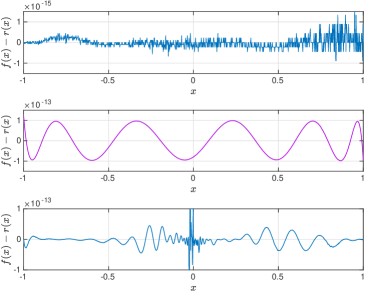
Figure 1: Illustration of aaax for rational approximation $r\approx f$ on $[-1,1]$, with each image showing the absolute error $f(x)-r(x)$ sampled at $1001$ equispaced points. Top: AAA approximation of $f(x)=e^{x}$ to default accuracy $10^{-13}$ ($1$ ms on our desktop, degree $6$). Middle: AAA-Lawson minimax approximation of $f(x)=e^{x}$ of degree $5$ ($5$ ms). Here and in other figures, AAA-Lawson error curves are distinguished by a purple color. Bottom: AAA approximation of $f(x)=|x|$ to requested accuracy $10^{-13}$ actually terminates with accuracy $1.3\times 10^{-12}$; see also Figures 7 and 8 ($600$ ms, degree $110$).

Figures 1 and 2 give an indication of the behavior of the continuum AAA algorithm and the template codes. (These and all our illustrations are based on our MATLAB rather than Julia codes, except in Figure 17.) The first image of Figure 1 shows the error in approximation of $e^{x}$ on $[-1,1]$ to the default tolerance of $10^{-13}$. The function call r = aaax(@exp) delivers a function handle r corresponding to a barycentric representation of a rational approximation of $f$ of degree 6, the computation taking less than a millisecond on a laptop (excluding plotting). The second line shows the error in minimax approximation of $e^{x}$ computed by r = aaax(@exp,5,20), which specifies rational degree 5 and 20 steps of AAA-Lawson iteration (our usual number). Note our convention of using a purple color to distinguish error curves obtained from AAA-Lawson computations. This computation takes about 5 ms; the Chebfun minimax code takes about 8 times as long. (All the timings in this paper are approximate.) The third line treats the classic example [26] of a more difficult function with a singularity, $f(x)=|x|$. Here the final degree is 110, corresponding to a much heavier computation, but still the execution is fast, about half a second. The approximation returned has maximal error about $1.3\times 10^{-12}$, which is not far from the theoretical minimum for an approximation of this degree, about $4\times 10^{-14}$ [30]. By contrast the Chebfun minimax code [12] fails above degree $82$, even though this is the most powerful Remez algorithm implementation available, and for this it requires four minutes to compute an approximation with the optimal error $3.1\times 10^{-12}$.

All these computations benefit crucially from the numerical stability of the barycentric representation of $r$, as is used by both AAA approximation and minimax. Varga, Ruttan, and Carpenter showed that if one works with the quotient representation $r(x)=p(x)/q(x)$, where $p$ and $q$ are polynomials, then computing a degree 80 approximation of $|x|$ requires 200-digit arithmetic [39]. The explanation of this instability is given in the discussion of Figure 5 in the next section; see also [12, 25].

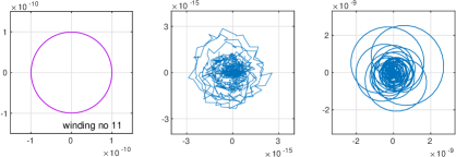
Figure 2: Illustration of aaaz for approximation on the unit circle, with each image showing the error curve $f(z)-r(z)$, where $z$ ranges over $1000$ equispaced points on the circle. Left: AAA-Lawson minimax approximation of $f(z)=e^{z}$ of degree $5$ ($12$ ms, error curve of winding number $11$). Middle: AAA approximation of $\sqrt{1-z^{-2}/4}$ to default accuracy $10^{-13}$ ($5$ ms, degree $12$). Right: AAA approximation of $\sqrt{1-z}$ again with default accuracy specification $10^{-13}$, though the code terminates at $10^{-9}$ ($110$ ms, degree $56$). In this last case the parameter mero is set to $0$, so the approximation is forced to be analytic in the unit disk.

Figure 2 gives a similar illustration of aaaz for complex approximation on the unit circle. The first image shows degree 5 minimax approximation of $e^{z}$, with an error curve $(f-r)(|z|=1)$ that looks perfectly circular. Near-circularity of error curves is a general phenomenon in complex minimax approximation, and for this example the exact error curve is circular to about one part in $10^{12}$ [31, 32]. The second image shows AAA approximation to the default tolerance of $f(z)=\sqrt{1-z^{-2}/4}$, a function that is analytic on the unit circle but has branch points at $z=\pm 1/2$. For this approximation the flag mero, to be discussed in Section 3, has been set to $1$ to allow poles in the unit disk; thus we are truly approximating on the circle, not the disk. The third image shows AAA approximation of $f(z)=\sqrt{1-z}$, which has a singularity on the unit circle. This time mero has been left at its default value $0$, forcing the approximation to be analytic in the unit disk. The reason the accuracy is only $10^{-9}$ is that after this point, the AAA iteration produced a string of approximations with poles in the unit disk, so the code has reverted to its best approximation found so far that is pole-free in the disk, as will be discussed in Section 2.

The next four sections present the details of continuum AAA on the unit interval, the unit circle or disk, the imaginary axis or right half-plane, and other real and complex domains. Many examples are shown along the way. Section 6 discusses certain challenges faced by the algorithm. The final section summarizes various aspects of continuum AAA approximation and its prospects. Our current algorithm is certainly not the last word on this subject, but it appears to be a substantial advance over what has been available before.

We would like to conclude this introduction with some comments on the relationship between minimax approximations, which can be computed by the AAA-Lawson variant, and near-minimax approximations, computed by AAA without Lawson.

Minimax approximations are undeniably fascinating. In real approximation, they are characterized by equioscillatory error curves, and in complex approximation they feature the complex analogue shown in Figure 2, error curves that are nearly circular, sometimes so close to circular that the variation of modulus could not be detected in floating point arithmetic. This makes minimax approximations beautiful, memorable, and easily recognized at a glance.

Partly for this reason, there has been a strong emphasis in the field of approximation theory on best as opposed to near-best approximations. This emphasis has been amplified by the fact that approximation theory, although it has always had its numerical practitioners, has been dominated by theorists.

We argue that for applications, minimax approximation should not normally be the starting point. The basic reason is one of practicality. Nobody knows how to compute minimax approximations as quickly and reliably as near-minimax ones. In the case of AAA approximation, adding a Lawson phase typically roughly doubles the computation time for the benefit of typically gaining just about a digit of accuracy, and with a greater risk of failure. (The size of the gain can be judged by noting the gaps between the green circles and the blue dots above them in Figures 4, 5, 9, and 11 below.) In particular, AAA-Lawson will almost always fail if one is dealing with approximations of accuracy close to machine precision. Thus in practice, as in the first two panes of Figure 1, one is often forced to choose between a non-optimal approximation of accuracy close to machine precision and an “optimal” approximation of lower accuracy! (The latter has lower degree.)

To put it another way, even if we keep well away from machine precision, the practical difference between minimax and near-minimax approximations is not that the former achieves slightly better accuracy, but that it achieves a prescribed accuracy with a slightly lower degree. This benefit is a modest one, easily outweighed by a reduction in speed and robustness.

2 Continuum AAA on $[-1,1]$

The precise specification of our algorithm can be found in the MATLAB code of the Appendix, particularly the $32$ lines labeled “Main AAA loop.” In this section we discuss the essential features, assuming the reader already has some familiarity with AAA [25].

The highest level description of the algorithm is as follows. At each step we have a row vector $S=[s_{1},\dots,s_{m}]$ of $m$ support points in $[-1,1]$ and a column vector $X=[x_{1},\dots,x_{N}]^{T}$ of $N=3(m-1)$ sample points in $[-1,1]\backslash S$, three equispaced sample points between each pair of support points. The sample points are constructed from $S$ by a function $X=\hbox{\tt XS}(S)$.

$S=[-1,1]$
for $m=2,3,\dots$ until convergence
   $(1)$ $X:=\hbox{\tt XS}(S)$
   $(2)$ Use SVD to compute barycentric weights for next approximation $r\approx f$
   $(3)$ $S:=S\cup\{\hbox{a sample point $x_{i}\in X$ where $|f(x_{i})-r(x_{i})|$ is maximal\/}\}$
end

Step (2) is the linearized least-squares computation introduced in [25], involving an $N\times m$ Loewner matrix $A$ with entries

(1) $$a_{ij}={f(x_{i})-f(s_{j})\over x_{i}-s_{j}}.$$

If the $m$-vector $w$ is a minimal singular vector of $A$, then

(2) $$\|Aw\|_{2}=\hbox{minimum},\quad\|w\|_{2}=1,$$

or equivalently,

(3) $$\|fd-n\|_{2}=\hbox{minimum},\quad\|w\|_{2}=1,$$

where $n$ and $d$ are the numerator and denominator of the barycentric quotient

(4) $$r(x)=\sum_{j=1}^{m}{w_{j}f(s_{j})\over x-s_{j}}\left/\sum_{j=1}^{m}{w_{j}\over x-s_{j}}\right..$$

In both (2) and (3), $\|\cdot\|_{2}$ is the discrete $2$-norm over $X$.

Step (3) amounts to greedy selection of the next support point, the standard nonlinear step of AAA approximation.

Step (1) is the feature that distinguishes continuum AAA from its fixed-grid predecessor. At each iterative step, the vector $X$ is determined by the current vector $S$ of support points. From one step to the next most sample points stay the same, except in the interval between the two support points where a new support point $s_{\hbox{\scriptsize new}}$ has been introduced in step (3); let us call this interval $(s_{j},s_{j+1})$. At step (1) the three sample points in $(s_{j},s_{j+1})$ are removed and six new sample points are added, three in $(s_{j},s_{\hbox{\scriptsize new}})$ and three in $(s_{\hbox{\scriptsize new}},s_{j+1})$.

In fact, we have slightly simplified the description of step (1). Inspection of the code XS will show that it takes not one but two arguments, $X=\hbox{\tt XS}(S,p)$, so that an arbitrary number $p$ of sample points will be placed between each pair of support points. The code aaax sets $p=\max\{3,16-m\}$ at step $m$, so that $p$ begins at $p=14$ for $m=2$ and reduces linearly with $m$ until it hits $p=3$ for $m\geq 13$. This is an engineering adjustment to ensure that the function $f$ is sampled at dozens of points during the approximation process, rather than as few as $3$ points. Such precautions have been been a familiar feature of adaptive numerical algorithms since the first adaptive integrators were introduced in the 1960s.

The other feature of the algorithm to be spelled out is the convergence criterion. The iteration stops if the maximum norm relative error on the sample points falls below a prescribed value tol, set by default to $10^{-13}$. The actual maximum error over all of $[-1,1]$ will be slightly larger, and this is checked a posteriori by evaluation on the finer grid $\hbox{\tt XS}(S,30)$. (If function evaluations are expensive, this step can be modified.) The iteration also stops if a prescribed maximum degree is reached, which is set by default to $150$. In addition the iteration stops if ten steps in a row have produced “bad poles,” that is, one or more poles in $[-1,1]$, and at least two digits of accuracy have been achieved. Poles are computed by means of a generalized eigenvalue problem by the prz code adapted from Chebfun; this is extremely fast and accurate, adding only about $25\%$ to the overall computation time even though poles are computed at every AAA step. In the case of termination due to bad poles, the approximation $r$ returned by aaax is the last one that was successfully computed without bad poles, so its accuracy will not be as good as $10^{-13}$. In practice we often find that a few digits are lost, but the approximation is always pole-free in the approximation interval.

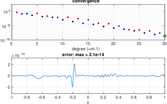
Figure 3: Plots produced by aaax in approximating $f(x)=\exp(-1/x^{2})$. The upper image shows convergence as a function of degree, with red dots marking steps with “bad poles”, i.e., poles in $[-1,1]$. The red-blue alternation is a result of $f$ being even. The second image shows the final error curve and maximal error on a finer grid. (Computation time excluding plotting: $20$ ms.)

In the default mode of operation, with an invocation as simple as r = aaax(f), the continuum AAA algorithm produces a pair of plots showing convergence and the final error curve. This is illustrated first in Figure 3 for a smooth function, $f(x)=\exp(-1/x^{2})$. Note that red dots are used to mark steps of the iteration with bad poles. The errors are measured on the sample grid; off the grid, the error in cases with bad poles would be $\infty$. The green circle in the upper plot, corresponding to the error value printed in the title of the lower plot, is the actual error as computed on the finer plotting grid.

If a second argument is provided to aaax, this is interpreted as the degree $m-1$ for the approximation (4) (more precisely a maximum degree, since the prescribed tolerance may be achieved earlier). Typically the result is an approximation whose error is on the order of a factor of ten or so greater than the minimax error for that degree. If a third argument is also provided, this is interpreted as a number of AAA-Lawson iterative steps to take in an attempt to improve the approximation to minimax. The 18 lines of Lawson code, which can be seen in the Appendix, are adapted from the algorithm introduced in [27]. We normally take 20 Lawson steps, and as discussed in [27], convergence occurs in the majority of cases so long as the error level is well above machine precision. Such a computation is illustrated in Figure 4, showing the result for degree 24 minimax approximation of the same function $f(x)=\exp(-1/x^{2})$ via aaax(@(x) exp(-1./x.^2,24,20)). A fourth argument to aaax allows one to adjust the convergence tolerance.

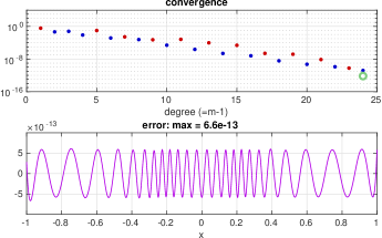
Figure 4: Approximation of the same function $f(x)=\exp(-1/x^{2})$, but now with the function call aaax(f,24,20) to specify maximal degree $24$ and $20$ AAA-Lawson steps. The result shows the expected equiosillation with an error of $6.6\times 10^{-13}$ ($25$ ms). The green circle lies below the final blue dot because AAA-Lawson has improved the error.

Figure 5 shows an example that is equivalent to a famous rational approximation problem, the degree $n$ rational approximation of $e^{s}$ for $s\in(-\infty,0\kern 0.3pt]$ first considered by Cody, Meinardus and Varga [5]. Setting $s=(x-1)/(x+1)$ transplants this to the problem of degree $n$ approximation of $\exp((x-1)/(x+1))$ for $x\in[-1,1]$. Executing aaax(@(x) exp((x-1)./(x+1)) produces Figure 5 in about $20$ ms of computing time. The same approximation can be computed by Chebfun minimax, taking about 100 times as long. For more on this problem see pp. 214–219 of [33].

The example of Figure 5 provides an illustration of the importance of the barycentric representation for numerical stability. If $r$ is written as a quotient of polynomials $p/q$ for this approximation, then $q$ decreases by a factor on the order of $10^{11}$ as $x$ moves from $1$ to $-1$, and $p$ decreases by a factor on the order of $10^{23}$. In floating point arithmetic, one would need a precision of more than 23 digits to retain any accuracy for $x\approx-1$. This effect gets rapidly more extreme at higher degrees.

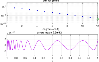
Figure 5: Approximation of $\exp((x-1)/(x+1))$ on $[-1,1]$, which is equivalent to the Cody–Meinardus–Varga problem of approximation of $\exp(s)$ on $(-\infty,0\kern 0.5pt]$ ($20$ ms). Here the degree $12$ AAA-Lawson result is computed.

Figure 6 considers approximation of the sigmoidal or Fermi–Dirac function $f(x)=1/(1+\exp(1000(x+0.5)))$ arising in electronic structure calculations, which makes a rapid transition from $f(x)\approx 1$ for $x<-0.5$ to $f(x)\approx 0$ for $x>-0.5$. A degree 38 rational approximation of accuracy $1.3\times 10^{-13}$ is obtained in 20 ms.  This appears to offer a big improvement over a recently published algorithm for this problem [24].

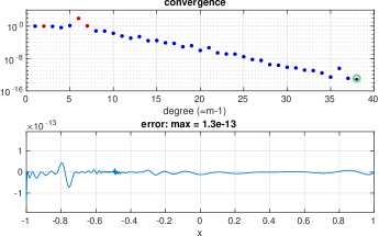
Figure 6: Approximation of the sigmoidal or Fermi–Dirac function $f(x)=1/(1+\exp(1000(x+0.5)))$ ($20$ ms).

Our final example of this section returns to the problem shown in Figure 1, approximation of $f(x)=|x|$. Figure 7 presents the convergence curve in this case, showing root-exponential convergence with approximately alternating blue and red dots (since $f$ is even) until at a level below $10^{-12}$, all the dots turn red and the iteration terminates. This successful computation of an approximation accurate to 12 digits in ordinary machine arithmetic happens in less than a second of computer time.

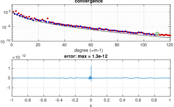
Figure 7: Approximation of the classic function with a branch point singularity, $f(x)=|x|$, showing root-exponential convergence as discovered by Newman [26]. $12$-digit accuracy is achieved in $600$ ms.  The black line under the data points shows the error of true minimax approximation.

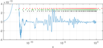
Figure 8: The error $f(x)-r(x)$ in continuum AAA approximation of $|x|$ on $[-1,1]$, plotted for $x\in(0,1]$ now on a semilogx scale. The dots show positions of support points in $(0,1]$ (black) and absolute values of conjugate pairs of zeros (green) and poles (red) near the imaginary axis.

It is known that the power of rational approximation for functions with singularities derives from exponential clustering of poles and zeros near these points [36]. The success of AAA for such problems depends on the support points being exponentially clustered too. Figure 8 illustrates how the continuum AAA computation of Figure 7 has achieved the necessary clusterings for all these three sets of points. The curve in the figure represents the error $f(x)-r(x)$ on the positive half of the domain, $x\in(0,1]$, and dots are placed on the same horizontal scale representing support points in $(0,1]$ (black), absolute values of zeros (green), and absolute values of poles (red). The poles and zeros lie approximately on the imaginary axis and in conjugate pairs, so each green and red dot has multiplicity $2$. It is evident that poles and zeros are (mostly) interlacing and exponentially clustered toward $x=0$, with the support points exponentially clustered in a similar manner. Towards $x=0$ the spacing between dots stretches out, the “tapering” effect analyzed in [36]. All this is computed blindly by the continuum AAA algorithm, which has no knowledge of optimality conditions or of the theory of exponential clustering.

Some problems of interest, such as those of Figures 4 and 7–8, involve functions $f(x)$ that are even or odd, and the algorithms could be modified to exploit this symmetry. We comment on exploitation of symmetry at the end of the next section.

3 Continuum AAA on the unit circle or disk

For approximation on the unit circle, our algorithm is mostly the same; the detailed changes can be seen in the code aaaz available in the Supplementary Materials.  Sample points are now placed between support points all around the circle with respect to angle, or equivalently, arc length. If AAA-Lawson is invoked, a numerical winding number is calculated since this is of interest for best and near-best approximations because of Rouché’s theorem. In the simplest case, if a function $f$ analytic in the disk has a degree $m-1$ rational approximation $r$ that is also analytic in the disk, and the error curve $(f-r)(|z|=1)$ is nearly a circle of winding number $\geq 2m-1$, then $\|f-r\|$ must be correspondingly close to minimal [32, Props. 2.1 and 2.2]. This is a complex analogue of the well-known de la Vallée Poussin lower bound in real approximation on an interval [33].

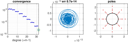
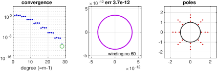
Figure 9: Continuum approximation of $f(z)=\tan(z^{4})$ on the unit circle. Upper row: aaaz(f) ($30$ ms). Lower row: aaaz(f,28,20) ($40$ ms). In the second case, in addition to the $24$ poles visible in the plot, there are four more with moduli about $6$.

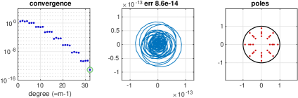
Figure 10: Approximation of $\tan(z^{-4})$ with the mero parameter set to $1$, so that poles of $r$ are permitted in the interior of the disk ($30$ ms).

Figure 9 illustrates aaaz approximation of $f(z)=\tan(z^{4})$. This function is analytic in the disk and meromorphic outside, with eight rays of poles extending to $\infty$. Continuum AAA achieves the prescribed accuracy by approximating the rays each by four poles. (Note that the errors in the convergence plot decrease in a staircase pattern because of the symmetry, a reflection of the Walsh table of best rational approximants to $f$ breaking into $4\times 4$ blocks of identical entries [33].) The innermost eight poles have moduli matching the value $(\pi/2)^{1/4}$ for $f$ to about 12 digits, and the next three rings of eight poles match the corresponding poles of $f$ to about 5, 2, and 1 digits, respectively. Similarly, the lower row of the figure shows an approximation to the same function with degree $28$ and $20$ steps of AAA-Lawson.

Although continuum AAA for the unit circle is like the algorithm for the unit interval, two new issues arise. The first is that the domain now encloses an interior, which raises the question, should the approximation $r$ be required to be analytic there? In other words, if a pole appears with $|z|<1$, should it be regarded as a bad pole? For some problems the answer will be yes, if an approximation analytic in the disk is sought, and in other cases it will be no, when we truly wish to approximate just on the circle. The code aaaz controls this choice with an input parameter mero (“meromorphic”), which by default is set to $0$. If $\hbox{\tt mero}=0$, then poles in the disk are treated as bad, following the same logic as described in the last section. If $\hbox{\tt mero}\neq 0$, then poles in the disk are accepted. (The possibility of poles exactly on the unit circle is unlikely enough in floating point arithmetic that we do not worry about it.)

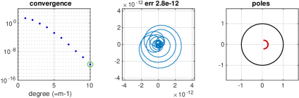
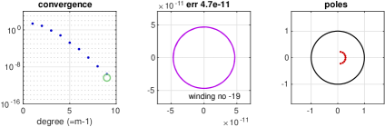
Figure 11: Approximation of $f(z)=\exp(4/z)$ on the unit circle, with an essential singularity at $z=0$. Upper row: aaaz(f) ($30$ ms). Lower row: aaaz(f,28,20) ($40$ ms).

Suppose, for example, we wish to approximate $f(z)=\tan(z^{-4})$ on the unit circle instead of $\tan(z^{4})$. With the default value $\hbox{\tt mero}=0$ this will result in failure (not shown), and indeed it is obvious that $\|f-r\|$ can be no less than $\tanh(1)\approx 0.76$ for a function $r$ analytic in the disk since $\tan(z^{-4})$ has winding number $-4$ on the unit circle and minimal modulus $\tanh(1)$, whereas an analytic function $r$ must have nonnegative winding number. (This is Rouché’s theorem again.) With $\hbox{\tt mero}=1$, however, the approximation is straightforward, and the result is shown in Figure 10, essentially a reflection in the unit circle of the upper row of Figure 9.

Figure 11 shows another pair of examples, near-minimax and minimax, involving the function $f(z)=\exp(4/z)$, which has an essential singularity at $z=0$. Although $f$ itself is not meromorphic in the unit disk, it is still analytic on the unit circle, and aaax with $\hbox{\tt mero}=1$ has no trouble constructing approximations.

Figure 12 shows approximation on the unit circle of $f(z)=|\hbox{\rm Re\kern 0.5pt}(z)|$, boundary data that cannot be matched by any function analytic inside or outside the disk. In the fashion familiar in the theories of Wiener–Hopf factorization and Riemann–Hilbert problems, however, it can still be regarded as the sum of one function analytic inside the disk plus another analytic outside (“analytic plus coanalytic”). As discussed in [7], AAA approximation may provide a valuable tool for such problems. The figure shows approximation to 13 digits by a rational function of degree 235, which has about 60 poles exponentially clustered on both sides of $z=i$ and $z=-i$. By separating the two sets of poles and switching to a partial fractions representation with coefficients determined by linear least-squares fitting, this can be the basis of very interesting further computations, including the solution of the Laplace or Stokes equations [6, 41].

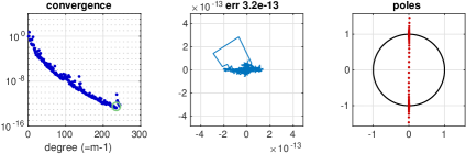
Figure 12: Approximation of $|\hbox{\rm Re\kern 0.5pt}(z)|$ on the unit circle with the mero parameter set to $1$, with exponentially clustered poles on both sides of $z=\pm i$ ($9$ s). Removing the poles inside or outside of the disk would be the first step towards a AAA-least squares computation as proposed by Costa [6, 7].

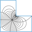
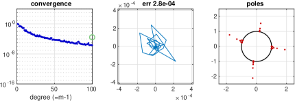
Figure 13: Conformal mapping example. The upper plot shows the conformal image in an L-shaped region of concentric circles and radial lines in the unit disk, as computed by the Schwarz–Christoffel Toolbox for MATLAB [11]. The lower image shows a degree $100$ continuum AAA rational approximation. The position of the green circle reflects a loss of accuracy near some of the vertices.

Figure 13 returns to functions analytic in the disk with an example from numerical conformal mapping. A conformal map $f$ of the unit disk onto a polygonal region can be represented as a Schwarz–Christoffel (SC) integral, and the standard software for computing such maps is the SC Toolbox for MATLAB [11]. As pointed out in [13], an effective strategy for representing SC maps numerically is rational approximation, taking advantage of poles exponentially clustered near corner singularities. The figure shows the result of degree $100$ rational approximation of a map onto an L-shaped region as generated by essentially this MATLAB code:

         v = [0 1i -1+1i -1-1i 1-1i 1];
         f = diskmap(polygon(v)); f = center(f,-.25-.25i); plot(f)
         r = aaaz(f,100);

Note that the poles of the approximant cluster exponentially near six “prevertices” along the unit circle. The accuracy is about 6 digits over most of the domain but falls to 4 digits very near the vertices (near five of them, to be precise). The rational approximation can be used to map points $z$ in the disk to their images in the L shape about ten times faster than with the SC Toolbox (about 1 ms vs. 10 ms per evaluation). As pointed out in [13], the ratio of speeds for evaluating the inverse map $f^{-1}$ typically exceeds $100$.

The other new feature that arises in approximation on the circle is the matter of real symmetry. A function $f$ is said to be real symmetric (or conjugate symmetric or Hermitian symmetric) if $\overline{f(z)}=f(\overline{z})$, and in such cases one might like to require the approximation $r$ to be real symmetric too. This is attractive not just cosmetically but also because exploiting the symmetry can provide a significant speedup.

Our template code aaax does not include an option to enforce real symmetry, and it breaks symmetry in two ways. First is simply by rounding errors. Second and more importantly, even in exact arithmetic, the sequence of support points will be nonsymmetric in general. One could modify the code to force symmetry at all stages, and various authors have done this [17, 20, 23, 37]. Other types of symmetry, most notably odd and even symmetry as mentioned at the end of the last section, could also be optionally enforced.

4 Continuum AAA on the imaginary axis or right half-plane

Many applications, especially in control theory and model order reduction, feature approximations $f(z)\approx r(z)$ on the imaginary axis, typically with a constraint that the poles should be in the left half-plane: in other words, $r$ should be analytic in the right half-plane. These problems can be regarded as transplants of approximation problems on the unit circle by a Möbius transformation. Specifically, the functions

(5) $$z=M\kern-1.0pt\left({1+w\over 1-w}\right),\quad w={z-M\over z+M}$$

describe a bijection of the unit disk in the $w$-plane and the right half of the $z$-plane, with $w=-1,0,1$ corresponding to $z=0,M,\infty$. As a practical matter, it might be desirable for a code to include $M$ as a parameter, since in an application one might happen to know that most of the action of $f(z)$ on the imaginary axis occurs, say, on the scale $|\hbox{\rm Im\kern 0.5pt}z|=O(10^{6})$ rather than $O(1)$. Our code arbitrarily fixes $M=1.207$, a choice close to $1$ but not equal to it so as to lead to fewer surprises since a pole $z=-M$ goes undetected because it is mapped to $\infty$ by the Möbius map.

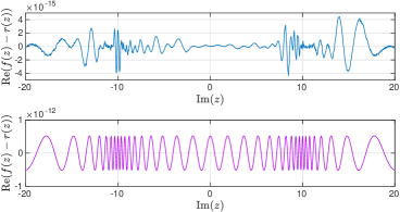
Figure 14: Errors in AAA approximation of $(\ref{twopts})$ on the imaginary axis to the default tolerance $10^{-13}$ ($25$ ms) and with degree $20$ and $20$ Lawson steps ($70$ ms). Both $f$ and the error $f-r$ are complex, and just the real part of the error is plotted.

Our template code aaai is a shell that calls aaaz after the transplantation (5). It has the same arguments f for the function, deg for the degree, nl for the number of AAA-Lawson iterations, tol for the tolerance, and mero to specify if a meromorphic approximation is permitted (i.e., with poles in the right half-plane as well as the left). We have not investigated continuum approximation on the imaginary axis in detail and give just two examples. Figure 14 shows near-minimax and minimax approximations to the function

(6) $$f(z)={1\over\sqrt{z-a}\kern 1.0pt\sqrt{z-\overline{a}\kern 0.5pt}\kern 1.0pt},\quad a=-1+10\kern 0.5pti.$$

This function has branch points at $z=-1\pm 10\kern 0.5pti$, and these are reflected in the denser error oscillations for $|\hbox{\rm Im\kern 0.5pt}z|\approx 10$. The figure shows the real part of the complex error $f(z)-r(z)$. For the second, minimax approximation the complex error curve describes a near-circle of winding number $35$ as $z$ traverses the imaginary axis downward from $+\infty\kern 0.5pti$ to $-\infty\kern 0.5pti$.

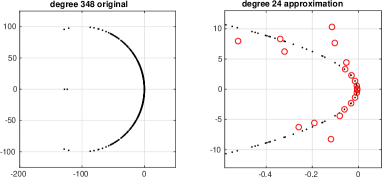
Figure 15: Poles in the complex plane for the clamped beam example from the NICONET collection [4]. On the left, the eigenvalues of the $348\times 348$ matrix $A$, which are the poles of its resolvent function. On the right, the poles of the degree $24$ AAA approximant computed with aaai. The poles near the imaginary axis are closely approximated, giving about $10^{-4}$ relative accuracy with (if symmetry is exploited) $72$ function evaluations.

The second example, shown in Figure 15, comes from the “clamped beam” problem from the NICONET collection of examples for model order reduction [4], which was also considered in Figures 6.13–6.14 of the original AAA paper [25]. The figure shows the poles of a continuum AAA approximation of degree $24$ with a relative error of about $10^{-4}$. For this problem, each function evaluation amounts to a scalarized resolvent, involving the inverse of a shift of a $348\times 348$ matrix $A$, and there are $144$ function evaluations. This number would be cut in half if real symmetry were exploited, so in effect we are getting 4-digit accuracy with about $72$ function evaluations as compared with the number $500$ used in [25]. The figure shows most of the 348 eigenvalues of $A$, on the left (a few are off-scale), and on the right, the 24 poles of the approximation $r$. The poles nearest the imaginary axis are captured closely, and their asymmetric configuration is a reminder that our codes do not enforce real symmetry.

In this section we have considered approximation on the imaginary axis, but of course, there are also problems posed on the real axis. Analogously, these may come with a requirement of analyticity in the upper or lower half-plane. These problems can be reduced to the former case by a multiplication by $i$ or $-i$.

5 Other real and complex domains

The algorithm we have presented extends readily to other domains. Approximation on ${\mathbb{R}}$ has just been mentioned. Approximation on a semiinfinite line like $[\kern 0.5pt0,\infty)$ can be treated by a Möbius transformation to $[-1,1]$, just as we used a transformation to the unit circle for approximation on the imaginary axis. Another real domain of interest in applications, going back to Zolotarev in the 19th century, is a pair of intervals $[a,b]\cup[c,d\kern 0.5pt]$. Here we would follow the algorithm essentially as described, with four initial support points $a,b,c,d$ and new support and sample points introduced in either $[a,b]$ or $[c,d\kern 0.5pt]$ at each step.

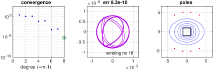
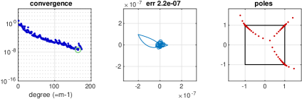
Figure 16: Rational approximations on the unit square. Upper row: degree $10$ continuum AAA approximation approximation of $\cos(4z)$ on the square and its interior with $20$ Lawson steps ($100$ ms). The error curve is nearly circular apart from four short portions near the corners of the square, where right angles are preserved since $(f-r)(z)$ is a conformal map. In the right image, error contours have been added to shown for $|f(z)-r(z)|=10^{-8},10^{-6},\dots,10^{0}$ (from inside out). Lower row: continuum AAA approximation of $f(z)=\min\{\hbox{\rm Re\kern 0.5pt}(z+1),\hbox{\rm Im\kern 0.5pt}(z+1)\}$ on the square without interior ($2.7$ ms). The absence of poles near $z=-1-i$ reveals that the algorithm has detected that there is no singularity there.

On complex domains we follow the pattern for the unit circle of working on the boundary contour, either with or without a requirement of analyticity in the interior (i.e., no poles). No essential change is needed in the algorithm, which can now distribute sample points according to arc length or (if the region is starshaped) the angle with respect to a center point. For our computed illustrations, we have modified aaaz into a code aaas for approximation on the unit square.

Figure 16 shows two examples. The first consists of degree $8$ approximation of $\cos(2x)$ on the square with $20$ Lawson steps. This would take $40$ ms, except that to get a better image we have run the Lawson iteration on a grid 10 times finer than usual: 20 SVD calculations involving matrices of dimension $4509\times 9$. This reveals an error curve that is nearly circular apart from four right angles. In the true minimax error curve, which emerges if one takes 200 rather than $20$ Lawson steps (not shown), the “double image” of the figure goes away as symmetry puts two parts of the error curve in exact superposition, a consequence of $\cos(2z)$ being an even function. The corresponding improvement in the error is from $8.3\times 10^{-10}$ to $8.0\times 10^{-10}$.

A striking application of rational approximation on complex domains is to the efficient representation of conformal maps, as mentioned in Section 3. In particular, the inverse Schwarz–Christoffel map from a polygonal region to the unit disk can be represented with great efficiency by rational functions [13].

The second row of Figure 16 shows an example in which the function to be approximated on the boundary of the square is real, making it necessary to approximate by a rational function with poles both inside and outside. The boundary function chosen, $f(z)=\min\{\hbox{\rm Re\kern 0.5pt}(z+1),\hbox{\rm Im\kern 0.5pt}(z+1)\}$, is zero on the left and bottom sides. Thus there is no singularity at the bottom-left corner, as the zero function is an analytic continuation to a neighborhood, and the AAA approximation reflects this in placing no poles near that corner. The other three corners have singularities, however, and the poles in the figure can be interpreted as delineating approximate branch cuts between the function branches $f_{1}(z)=0$ in the lower-left, $f_{2}(z)=z+1-i$ near the top, and $f_{3}(z)=1+i-iz$ near the right side. Such approximate branch cut effects are discussed, among other places, in [35]. As mentioned in connection with Figure 12, this kind of approximation with poles on both sides is the starting point of the AAA-least squares method introduced by Costa [6, 7].

6 Areas for improvement

The continuum AAA algorithm is remarkably fast and accurate for most approximation problems. Like its discrete predecessor, however, it is sometimes disappointing, especially in approximation of real functions with singularities. Here we discuss four issues with its behavior, confining our attention to this most challenging case, approximation by aaax of a real function $f(x)$ on $[-1,1]$.

1. Failure to meet the convergence tolerance. When $f$ is smooth, aaax typically converges in milliseconds to the default tolerance $10^{-13}$. For example, $f(x)=\tanh(100x)$ is approximated in 20 ms by a degree $30$ rational function with error $1.3\times 10^{-14}$. With $f(x)=\tanh(1000x)$, however, red dots appear for degree $\geq 45$, indicating the presence of bad poles, and the computation terminates with degree $43$ and error $1.6\times 10^{-11}$. This kind of “red zone termination” can be seen in Figure 7.

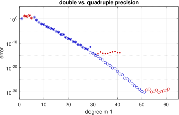
Figure 17: Comparison of double (dots) and quadruple precision (circles, computed in Julia) for $f(x)=\tanh(100x)$. Both iterations are run until ten steps in a row with bad poles have appeared.

We believe that in most cases, such failures are related to rounding errors in floating point arithmetic. This is confirmed by an experiment in quadruple precision Julia for $f(x)=\tanh(100x)$, shown in Figure 17, where convergence to accuracy $10^{-29}$ is readily achieved.

Of course, even if a failure would not occur in exact arithmetic, that does not mean that an algorithm is optimal. We hope that further developments will enhance the stability of continuum AAA further, so that it more reliably gets down to $10^{-13}$ in double precision arithmetic.

2. Zeroing in on singularities. Examining the behavior of continuum AAA for problems with singularities reveals that reasonably uniform error behavior is often not achieved near these points. In fact, trouble near singularities has already appeared in four of our figures. In Figures 1 and 7, both involving $f(x)=|x|$, there is a disconcerting spike in the final error curve. In Figure 13 (conformal map to L shape), the same kind of localized trouble shows up as a green circle two orders of magnitude above the blue dots, reflecting inaccuracy near prevertex square root singularities. It is the semilogx plot of Figure 8 that reveals the most. Here we see a much bigger error at the left side of the plot, off the vertical scale. The dots in this figure suggest that AAA would have done better to put one or two support points closer to the singularity at $x=0$. We see this in many experiments involving functions with singularities. Perhaps a modification of the algorithm might enhance its ability to zoom in speedily to difficult points, but we have not yet found the right trick.

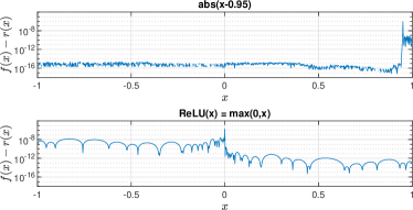
Figure 18: Illustrations of a difficulty that sometimes arises with the continuum AAA algorithm: the appearance of imbalances between the two sides of a singularity. The images show the final errors for $f(x)=|x-0.95|$ and $f(x)=\max(0,x)$. The errors $7.5\times 10^{-7}$ and $1.5\times 10^{-6}$ are much worse than the error $1.3\times 10^{-12}$ for the very similar function $f(x)=|x|$.

3. Asymmetries and oscillations. Another oddity that arises in certain cases is a pronounced asymmetry between the errors on the two sides of a singularity, which sometimes persists on the same side from step to step and sometimes oscillates from one side to the other (cf. Figure 6.1 of [27]). Figure 18 shows two examples, both of which ought to be straightforward variations of $f(x)=|x|$ but in fact are much less successful. In the first plot, for $f(x)=|x-0.95|$, the final error is ten orders of magnitude higher for $x>0.95$ than for $x<0.95$. Clearly something about the algorithm is out of balance. The second plot shows a similar imbalance in approximation of the function $f(x)=\max\{0,x\}$. The difficulty looks smaller in magnitude, but it stops convergence just as surely, and it is particularly embarrassing that our algorithm should do such a poor job on the famous “ReLU” function.

4. Bad poles. Finally there is the perennial question in AAA approximation—indeed, in rational approximation generally—of what to do when there are poles in a region where $r$ should be analytic. There is an established technology available for such problems, introduced in the AAA context in [17] and used by other authors in different settings (e.g. [7, 18]): one can switch from the barycentric representation to partial fractions, after first discarding or moving any unwanted poles. It is also possible to discard or move poles while retaining a barycentric representation [19, 20].

In the early stages of the research that led to this paper, we assumed that the switch to partial fractions would be an essential part of our algorithm. However, in the end we did not find enough situations where this was advantageous for us to make this a part of continuum AAA.  One reason to avoid partial fractions is that they bring a loss of elegance and clarity, since one ends up with an algorithm that delivers a rational function sometimes in one representation, sometimes in another. A more serious drawback is that there is usually a loss of several digits of precision. A third is that, since the poles of a partial fraction representation are fixed, one loses the possibility of improving a near-minimax fit to minimax by a Lawson iteration.

Our experiments show that in difficult cases, bad poles often arise in approximately alternate steps rather than in long sequences of steps, until one gets down to the “red zone termination” related to rounding errors as discussed above. In other words, there are usually enough blue dots for the algorithm to proceed to a successful conclusion. This need not always be the case, however, especially for functions with multiple singularities.

Another quite different approach to the bad poles problem is the “cleanup” procedure introduced in the original AAA paper [25], which has subsequently been refined by the third author and Costa (unpublished). Here, when a bad pole is encountered, the nearest support point is removed from $S$ and a new linearized least-squares fit is computed. Cleanup is not invoked in the algorithm described in the present paper, but perhaps it should ultimately play a role in the design of robust software.

7 Summary and discussion

We have introduced a continuum AAA algorithm for minimax and near-minimax rational approximation on real and complex sets, with template MATLAB and Julia programs for $[-1,1]$, the unit circle, and the imaginary axis. The algorithm delivers an approximation with no bad poles, which will usually have relative accuracy at the default tolerance level of $10^{-13}$. The speed is remarkable, with approximations typically produced in milliseconds. For approximation of degree $m$, the total number of function evaluations along the way is $\sim 6\kern 0.7ptm$.

Our template codes lie in the middle of the spectrum from pseudocode to software. We hope readers will download them from the Supplementary Materials or the authors’ web sites and enjoy successful explorations. In the interest of compactness and readability, however, our codes omit various features that one would expect in true software. The omission of an option to impose real symmetry was discussed in Section 3. Another example is that we have not structured the codes to avoid recomputation of values $f(z)$ at points $z$ where they have already been evaluated, which would be important for problems where evaluation of $f$ is expensive.

There does not appear to be much previous work on adaptive selection of sample points for barycentric rational approximation, but we note the important recent paper of Pradovera [28]. He recommends a strategy in which the next sample point is added at a point where the barycentric denominator is minimal.

The original, discrete AAA algorithm, whose standard implementation is the aaa code of Chebfun, remains fast and important. The simplest starting point in dealing with an approximation problem may be to simply fix a few thousand points in a set Z, evaluate $\hbox{\tt F}=f(\hbox{\tt Z})$, and call aaa(F,Z). This is certainly the way to go with exotic sets, such as mixtures of discrete and continuum components, and it also works for approximating functions that are meromorphic rather than analytic in the approximation domain, with poles amidst the sample points. When one is truly working on a continuum, however, continuum AAA will be more reliable, both because the adaptive selection of points can bring more speed and accuracy and also, very importantly, because of the guarantee that the result will be free of bad poles.

Rational approximation problems are of urgent importance in applied areas including signal processing and model order reduction, and more recently, solution of PDEs. We are well aware that this paper is a long way from such applications, focusing on basic algorithms in the setting of real and complex approximation theory.

With continuum AAA, is it now feasible to develop a system for numerical computation based on rational functions, just as Chebfun makes use of polynomials and piecewise polynomials? This is a question on our minds for ongoing work.

8 Appendix: MATLAB and Julia code templates

Here are listings of the main MATLAB template code aaax for continuum AAA approximation on $[-1,1]$ and the three functions XS, prz, and reval, the last two adapted from Chebfun. These codes are intended to be read as well as executed, with careful comments in the mathematical sections but a rougher uncommented style in the plotting sections.

The similar codes aaaz and aaai for the unit circle and the imaginary axis, respectively, are available in the Supplementary Materials, together with Julia equivalents of everything. The Julia codes offer the option of computation in quadruple precision.

function [r,pol,res,zer,err,S] = aaax(f,deg,nl,tol,plt)
%AAAX   Rational approximation on [-1,1].
%   [r,pol,res,zer,err,S] = aaax(f,deg,nlawson,tol,plt)
%Examples:
%   aaax(@exp); aaax(@exp,5); aaax(@exp,5,20);
%   [r,pol] = aaax(@(x) tanh(20*pi*x)); pol
%   aaax(@abs,150,0,1e-10);

                                               % INITIALIZATIONS
if nargin<2, deg = 150; end                    % arg 2: (max) degree
if nargin<3, nl = 0; end                       % arg 3: Lawson steps, eg 20
if nargin<4, tol = 1e-13; end                  % arg 4: relative tolerance
if nargin<5, plt = 1; end                      % arg 5: plt=0 stops plotting
blue = [0 0 .8]; red = [.8 0 0];
grn = [.5 .8 .5];  MS = ’markersize’;
CO = ’color’; LW = ’linewidth’;
S = [-1 1];                                    % row vector of support pts
f0 = f([S’; XS(S,10)]); err = std(f0);
if (err==0) | (err/abs(mean(f0))<=tol) ...     % constant function or deg 0:
            | (deg==0)                         % return (no plot)
   r = @(x) mean(f0) + 0*x; return
end
m0 = 2; S0 = S; w0 = [1; -1]; err0 = err;

while true                                     % MAIN AAA LOOP
   m = length(S);
   X = XS(S,max(3,16-m));                      % column vector of sample pts
   C = 1./(X-S);                               % Cauchy matrix
   A = (f(X)-f(S)).*C;                         % Loewner matrix
   [~,~,V] = svd(A,0);                         % SVD
   w = V(:,end);                               % barycentric wt vector
   R = (C*(w.*f(S’)))./(C*w);                  % rat approx at sample pts
   err = norm(f(X)-R,inf);                     % abs error of this approx
   pol = prz(S’,f(S’),w);                      % poles
   bad = any(imag(pol)==0 & abs(pol)<=1);      % check for bad poles
   co = blue;
   fmax = norm(f([S’;X]),inf);
   if ~bad & err < err0
      m0 = m; S0 = S; w0 = w; err0 = err;      % save latest success
   end
   if plt
      subplot(211), if bad, co = red; end
      semilogy(m-1,err,’.’,MS,10,CO,co), hold on
      title convergence, ylim([1e-16 1e4]), grid on
      set(gca,’ytick’,10.^(-16:8:0)), xlabel(’degree (=m-1)’)
   end
   if ~bad & (err/fmax<=tol) | ...             % stop if converged
      (m == deg+1) | ...                       % stop if max degree reached
      ((m-m0>=10) & (err0/fmax<1e-2))          % stop if stagnated
      break
   end
   [~,j] = max(abs(f(X)-R)); S = [S X(j)];     % next support point
end
m = m0; S = S0; w = w0; err = err0;
[pol,res,zer] = prz(S’,f(S’),w);
r = @(x) reval(x,S’,f(S’),w);                  % function handle for r

if nl > 0                                      % LAWSON ITERATION
   X = XS(S,20); n = length(X);                % switch to finer grid
   wt = ones(m+n,1);                           % Lawson wt vector
   C = 1./(X-S);                               % Cauchy matrix
   R = (C*(w.*f(S’)))./(C*w);                  % rat approx at sample pts
   F = [f(X); f(S’)]; R = [R; f(S’)];          % f and r values
   L = f(X).*C;
   A = [C; eye(m)]; B = [L; diag(f(S))];       % numer and f*denom rows
   for stepno = 1:nl                           % take nl Lawson steps
      [~,~,V] = svd(sqrt(wt).*[A B/fmax],0);
      c = V(:,2*m);
      a = c(1:m); w = -c(m+1:2*m)/fmax;        % numer wts, denom wts
      R = (A*a)./(A*w);
      wt = wt.*abs(F-R);                       % iterative reweighting
      wt = wt/norm(wt,inf);
   end
   r = @(x) reval(x,S’,a./w,w);                % function handle for r
end

xx = sort([XS(S,30); S’]);                     % COMPUTE ERROR AND PLOT
ee = f(xx)-r(xx); err = norm(ee,inf);
if plt
   semilogy(m-1,max(err,1e-16),’o’,LW,2,CO,grn)
   hold off, subplot(212), co = [0 .45 .74];
   if nl > 0, co = [.7 0 .9]; end, plot(xx,ee,LW,.7,CO,co)
   s = sprintf(’error: max =%8.1e’,err); ylim(1.5*(err+realmin)*[-1 1])
   title(s), grid on, xlabel x
end
end

function XS = XS(S,p)                          % SAMPLE POINTS
S = sort(S); d = (1:p)/(p+1);
XS = S(1:end-1) + d’.*diff(S);
XS = XS(:);
end

function [pol,res,zer] = prz(xj,fj,wj)         % POLES, RESIDUES, ZEROS
m = length(wj);                                %    (from Chebfun)
if any(wj==0)
   ii = find(wj~=0); m = length(ii);
   xj = xj(ii); fj = fj(ii); wj = wj(ii);
end
B = eye(m+1); B(1,1) = 0;
E = [0 wj.’; ones(m,1) diag(xj)];
pol = eig(E,B); pol = pol(~isinf(pol));
if nargout >= 2
   N = @(t)(1./(t-xj.’))*(fj.*wj);
   Ddiff = @(t) -((1./(t-xj.’)).^2)*wj;
   res = N(pol)./Ddiff(pol);
   E = [0 (wj.*fj).’; ones(m,1) diag(xj)];
   zer = eig(E,B); zer = zer(~isinf(zer));
end
end

function r = reval(zz,xj,fj,wj)                % FUNCTION HANDLE FOR R
z = zz(:); C = 1./(z-xj.’);                    %    (from Chebfun)
r = (C*(wj.*fj))./(C*wj);
r(isinf(z)) = sum(wj.*fj)./sum(wj);
ii = find(isnan(r));
for j = 1:length(ii)
   r(ii(j)) = fj(z(ii(j))==xj);
end
r = reshape(r,size(zz));
end

References

- [1] A. C. Antoulas, C. A. Beattie, and S. Güğercin, Interpolatory Methods for Model Reduction, SIAM (2020).
- [2] A. Budiša, X. Hu, M. Kuchta, K.-A. Mardal, and L. Zikatanov, Rational approximation preconditioners for multiphysics problems, arXiv:2209.11659v2 (2022).
- [3] A. Carracedo Rodriguez, L. Balicki, and S. Güğercin, The p-AAA algorithm for data driven modeling of parametric dynamical systems, arXiv: 2003.06536v3 (2022).
- [4] Y. Chahlaoui and P. Van Dooren, A Collection of Benchmark Examples for Model Reduction of Linear Time Invariant Dynamical Systems, EPrint 2008.22, Manchester Institute for Mathematical Sciences, University of Manchester, Manchester, 2002.
- [5] W. J. Cody, G. Meinardus, and R. S. Varga, Chebyshev rational approximations to in and applications to head-conduction problems, J. Approx. Thy., 2 (1969), pp. 50–65.
- [6] S. Costa, E. Costamagna, and P. Di Barba, Permanent magnet models with rational approximations, manuscript submitted to ISEF 2023 (Pavia), 2023.
- [7] S. Costa and L. N. Trefethen, AAA-least squares rational approximation and solution of Laplace problems, Proceedings 8ECM, to appear.
- [8] E. Deckers, S. Jonckheere, and K. Meerbergen, Time integration of finite element models with nonlinear frequency dependencies, arXiv:2206.09617 (2022).
- [9] G. Deng and C. J. Lustri, Exponential asymptotics of woodpile chain nanoptera using numerical analytic continuation, Stud. Appl. Math., 150 (2023), pp. 520–557.
- [10] N. Derevianko, G. Plonka, and M. Petz, From ESPRIT to ESPIRA: estimation of signal parameters by iterative rational approximation, IMA J. Numer. Anal., 43 (2023), pp. 789–827.
- [11] T. Driscoll, Schwarz-Christoffel Toolbox for conformal mapping in MATLAB, version 3.1.3, 2021.
- [12] S.-I. Filip, Y. Nakatsukasa, L. N. Trefethen, and B. Beckermann, Rational minimax approximation via adaptive barycentric representations, SIAM J. Sci. Comput., 40 (2018), A2427–A2455.
- [13] A. Gopal and L. N. Trefethen, Representation of conformal maps by rational functions, Numer. Math., 142 (2019), pp. 359–382.
- [14] I. V. Gosea and S. Güttel, Algorithms for the rational approximation of matrix-valued functions, SIAM J. Sci. Comput., 43 (2021), pp. A3033–A3054.
- [15] S. Güttel, G. M. Negri Porzio, and F. Tisseur, Robust rational approximations of nonlinear eigenvalue problems, SIAM J. Sci. Comput., 44 (2022), A2439–A2463.
- [16] T. Haut, G. Beylkin, and L. Monzón, Solving Burgers’ equation using optimal rational approximations, Appl. Comp. Harm. Anal., 24 (2013), pp. 39–95.
- [17] A. Hochman, FastAAA: A fast rational-function fitter, in 2017 IEEE 26th Conference on Electrical Performance of Electronic Packaging and Systems (EPEPS), IEEE (2017), pp. 1–3.
- [18] D. Huybrechs and L. N. Trefethen, AAA interpolation of equispaced data, BIT Numer. Math., 2023.
- [19] W. R. Johns, Multi Input Minimax Adaptive Antoulas-Anderson Algorithm for Rational Approximation with Stable Poles, PhD dissertation, Montana State U., 2021.
- [20] W. R. Johns, Iterative stability enforcement in AAA algorithms for H2 model reduction, SIAM J. Sci. Comput., to appear.
- [21] B. Keith, U. Khristenko, and B. Wohlmuth, A fractional PDE model for turbulent velocity fields near solid walls, J. Fluid Mech., 916 (2021), pp. A21-1–30.
- [22] P. Lietaert, K. Meerbergen, J. Pérez, and B. Vandereycken, Automatic rational approximation and linearization of nonlinear eigenvalue problems, IMA J. Numer. Anal., 42 (2022), pp. 1087–1115.
- [23] The MathWorks, Inc., RF Toolbox, https://www.mathworks.com.
- [24] E. Moussa, Minimax rational approximation of the Fermi–Dirac distribution, J. Chem. Phys., 145 (2016), 164108.
- [25] Y. Nakatsukasa, O. Sète, and L. N. Trefethen, The AAA algorithm for rational approximation, SIAM J. Sci. Comput., 40 (2018), pp. A1494–A1522.
- [26] D. J. Newman, Rational approximation to , Mich. Math. J., 11 (1964), pp. 11–14.
- [27] Y. Nakatsukasa and L. N. Trefethen, An algorithm for real and complex rational minimax approximation, SIAM J. Sci. Comput., 42 (2020), pp. A3157–A3179.
- [28] D. Pradovera, Toward a certified greedy Loewner framework with minimal sampling, arXiv:2303.01015v1 (2023).
- [29] Y Saad, M. El-Guide, and A. Miedlar, A rational approximation method for the nonlinear eigenvalue problem, arXiv:1901.01188v2 (2020).
- [30] H. Stahl, Best uniform rational approximation of on , Russian Acad. Sci. Sb. Math., 76 (1993), pp. 461–487.
- [31] L. N. Trefethen, Near-circularity of the error curve in complex Chebyshev approximation, J. Approx. Thy., 31 (1981), pp. 344–367.
- [32] L. N. Trefethen, Rational Chebyshev approximation on the unit disk, Numer. Math., 37 (1981), pp. 297–320.
- [33] L. N. Trefethen, Approximation Theory and Approximation Practice, Extended Edition, SIAM, 2019.
- [34] L. N. Trefethen, Numerical conformal mapping with rational functions, Comp. Meth. Funct. Thy., 20 (2020), pp. 369–387.
- [35] L. N. Trefethen, Numerical analytic continuation, Japan J. Appl. Math., submitted.
- [36] L. N. Trefethen, Y. Nakatsukasa, and J. A. C. Weideman, Exponential node clustering at singularities for rational approximation, quadrature, and PDEs, Numer. Math., 147 (2021), pp. 227–254.
- [37] A. Valera-Rivera and A. E. Engin, AAA algorithm for rational transfer function approximation with stable poles, Lett. Electr. Compatibility Prac. and Applics., 3 (2021), pp. 92–95.
- [38] R. S. Varga and A. J. Carpenter, On the Bernstein conjecture in approximation theory, Constr. Approx., 1 (1985), pp. 333–348.
- [39] R. S. Varga, A. Ruttan, and A. J. Carpenter, Numerical results on best uniform approximation of on , Math. USSR-Sb., 74 (1993), pp. 271–290.
- [40] H. Wilber, A. Damle, and A. Townsend, Data-driven algorithms for signal processing with trigonometric rational functions, SIAM J. Sci. Comput., 44 (2022), pp. C185–C209.
- [41] Y. Xue, et al., Computation of 2D Stokes flows via lightning and AAA rational approximation, Trefethen in preparation.