Supporting Information
Machine learning for accelerated bandgap prediction
in strain-engineered quaternary III-V semiconductors

ML		: Machine learning
SVM-RBF model		: Support Vector Machine with Radial Basis Function kernel machine learning model
SVR-RBF model		: Support Vector Regression with Radial Basis Function kernel machine learning model
SVC-RBF model		: Support Vector Classification with Radial Basis Function kernel machine learning model
RMSE		: Root Mean Squared Error
MAE		: Mean Absolute Error
Max error		: Maximum error
R2		: Coefficient of determination

S1.   Hyperparameter optimization

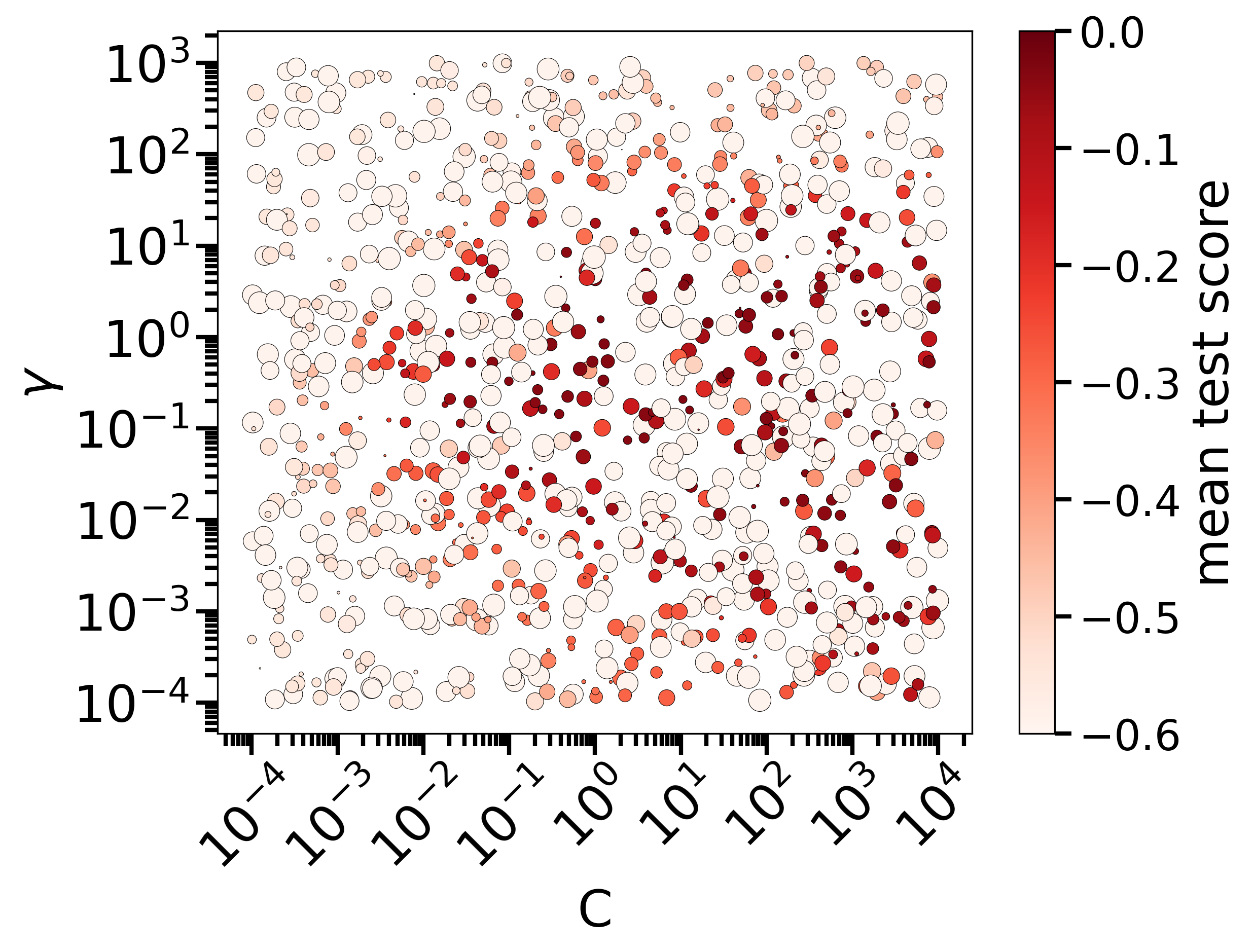
(a) $\varepsilon=10^{-3}-10^{2}$

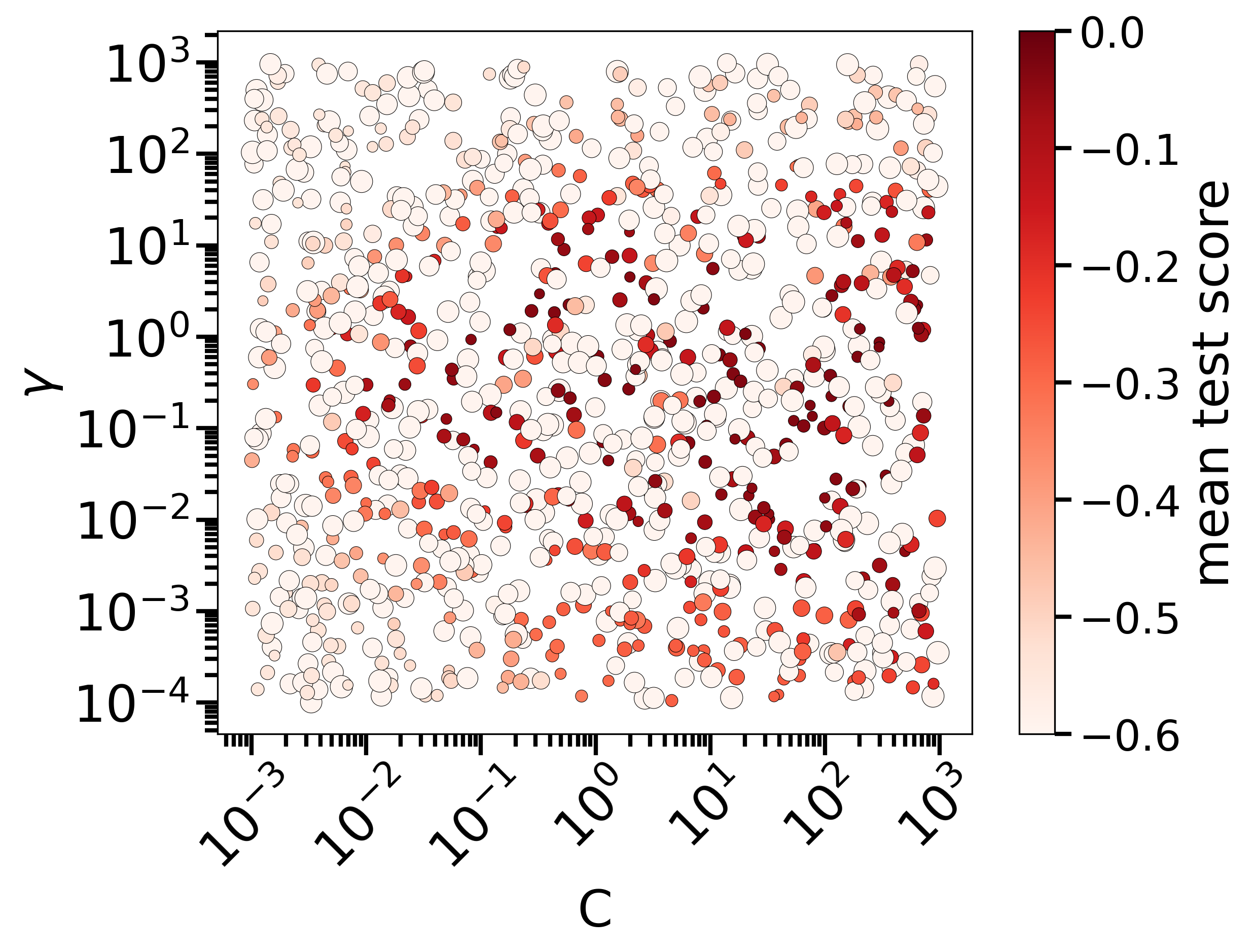
(b) $\varepsilon=10^{-2}-10^{2}$

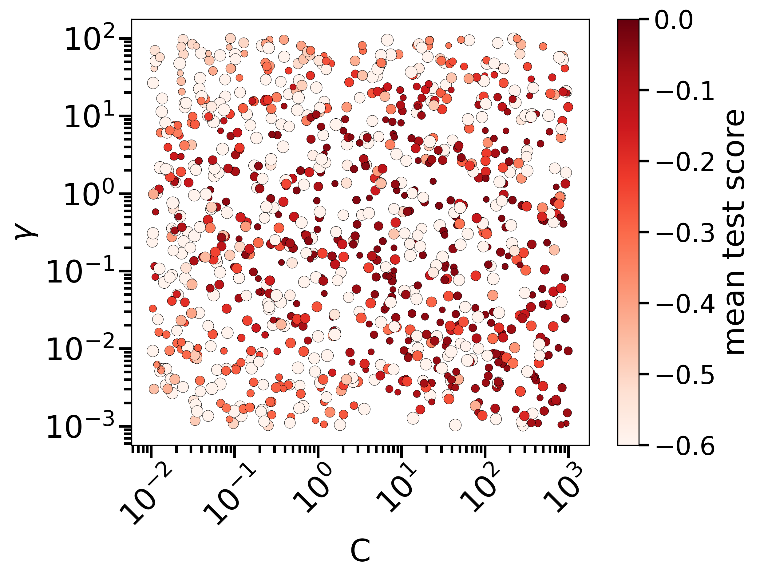
(c) $\varepsilon=10^{-2}-10$

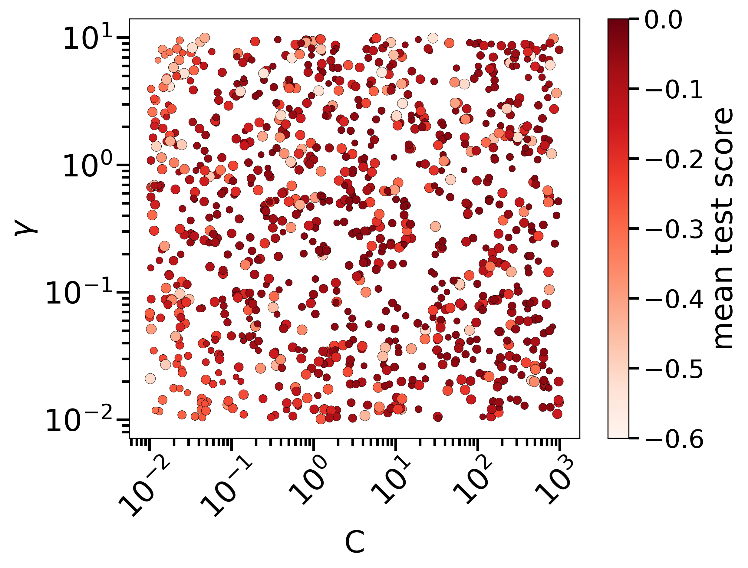
(d) $\varepsilon=10^{-2}-1$

Figure S1: Hyperparameter optimization with the largest dataset (3210 training data points) using random search cross-validation of the SVR-RBF model. The hyperparameter optimization scoring function is the negative RMSE, meaning that a small error or a high test-score (red) is beneficial. The random search is performed for each subfigure over 1000 random $C$, $\gamma$, and $\varepsilon$ combinations from a logarithmic uniform distribution space. The sizes of the circles, depicted in $\log$-scale, represent the $\varepsilon$ values. Specifically, we plot $\log(10^{3}\varepsilon)$ values to ensure non-negative marker size. The ranges for $C$, $\gamma$, and $\varepsilon$ are made tighter from (a) to (d).

In Fig. S1, we show the hyperparameter optimization with random search cross-validation of the SVR-RBF model. We tune the $C$, $\gamma$, and $\varepsilon$ ranges and find Fig. S1d as the optimal choice, covering the regimes with the best hyperparameters set. The larger $C$ value ($>10^{3}$) would result in a hard margin in the SVR model and, thus, poor generalization on unknown data. Therefore, for $C$, no larger values are sampled here.

Note the mean test score values in Fig. S1 are displayed on a negative scale. As mentioned in the manuscript, we used the package sklearn for implementing the ML models in this article. The hyperparameter optimizations in this package are performed by evaluating the scoring function values over the cross-validation set. In sklearn, by convention, the convention is to maximize all scorer objects during optimization. However, in ML problems, the objective is to minimize the error for error functions. Thus metrics such as ‘mean squared error’ are available as ‘negative mean squared error’ in hyperparameter optimization scoring functions, which return the negated value of the metric.

S2.   Negative direct bandgap

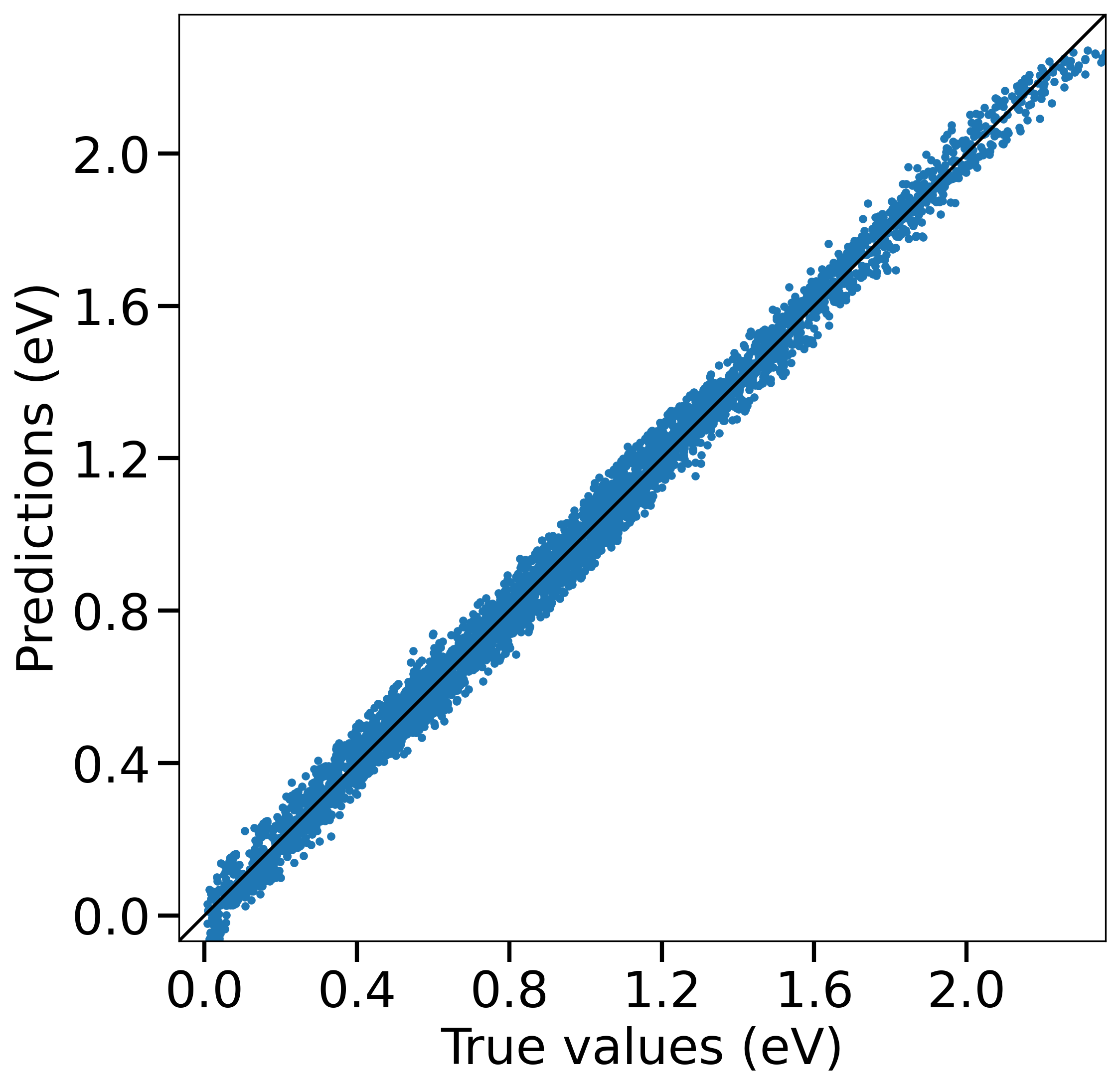
Figure S2: The SVR-RBF model bandgap value predictions over all the samples. The true values are the DFT calculated bandgaps. The hyperparameters are optimized with RMSE metric.

In Fig. S2, the bandgap values were predicted using SVR-RBF model. The hyperparameters of the model were optimized using RMSE metric, Eq. S1. However, the corresponding SVR-RBF model predicted a few small negative direct bandgap values of up to –5 meV (see left-bottom corner in Fig. S2). In the manuscript, we thus converted all the predicted negative bandgap values ($\hat{y}_{i}$) to 0 ($\hat{y}_{i}$=0). The RMSE of the model predictions was calculated after the conversion. Accordingly, all the performance metrics evaluated did include this conversion.

$$\text{RMSE}=\sqrt{\frac{1}{n_{{}_{\text{samples}}}}\sum_{i=1}^{n_{{}_{\text{samples}}}}\left(y_{i}-\hat{y}_{i}\right)^{2}}$$ (S1)

Where $\hat{y}_{i}$ is the ML model predicted value of $i$-th sample and $y_{i}$ is the corresponding true value. $n_{{}_{\text{samples}}}$ is the total number of samples.

S3.   Machine learning dataset features and labels for GaAsPSb

The full data dataset can be found in the Supplementary Information attachment. In the table below, the ML features for 3 example data are given.
Sample 1: Ga₁₀₀P₀As₁₀₀Sb₀ ($\equiv$ GaAs), unstrained
Sample 2: Ga₁₀₀P₂₅As₂₅Sb₅₀, 3.0% biaxial tensile strained
Sample 3: Ga₁₀₀P₅₀As₅₀Sb₀, 5.0% biaxial compressively strained

Sample index	Features				Labels
	Phosphorus (%)	Arsenic (%)	Antimony (%)	Strain (%)	Bandgap value (eV)	Bandgap nature
1	0	100	0	0.0	1.466	direct
2	25	25	50	3.0	0.629	direct
3	50	50	0	-5.0	1.243	indirect

S4.   Dataset convergence

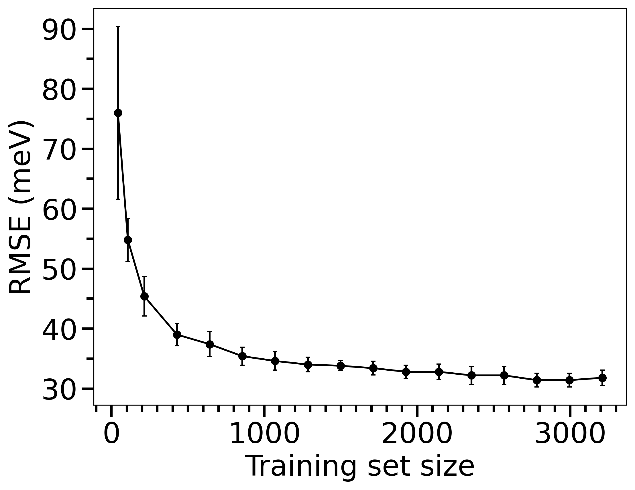
(a)

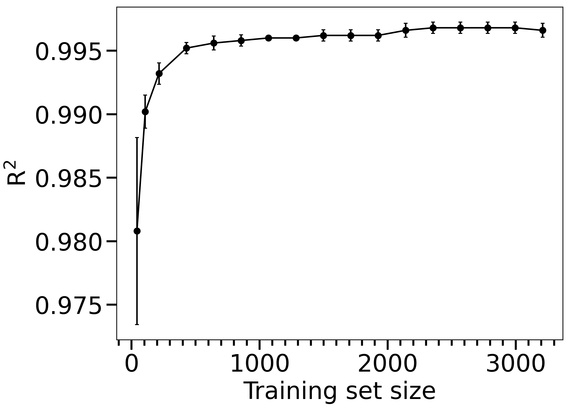
(b)

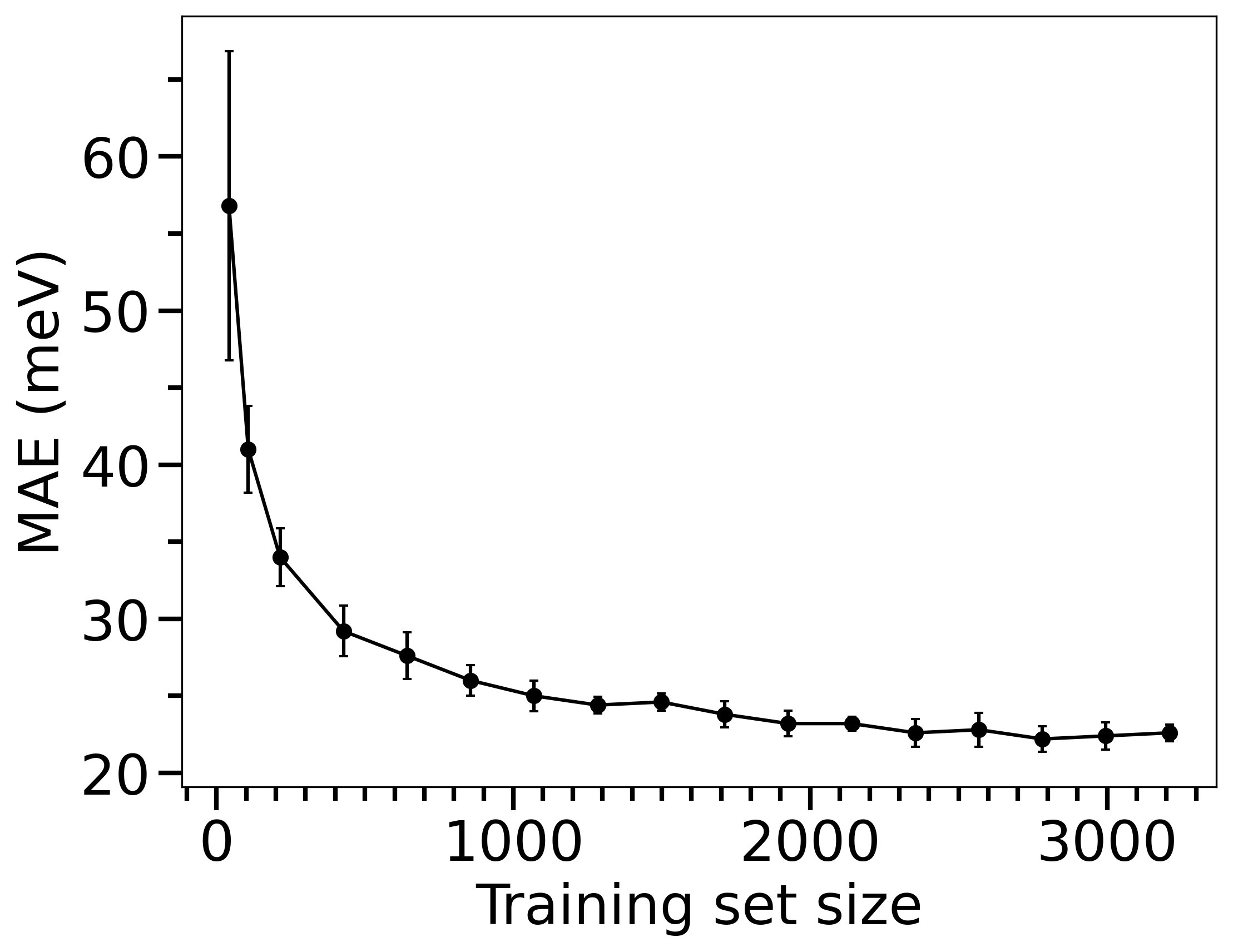
(c)

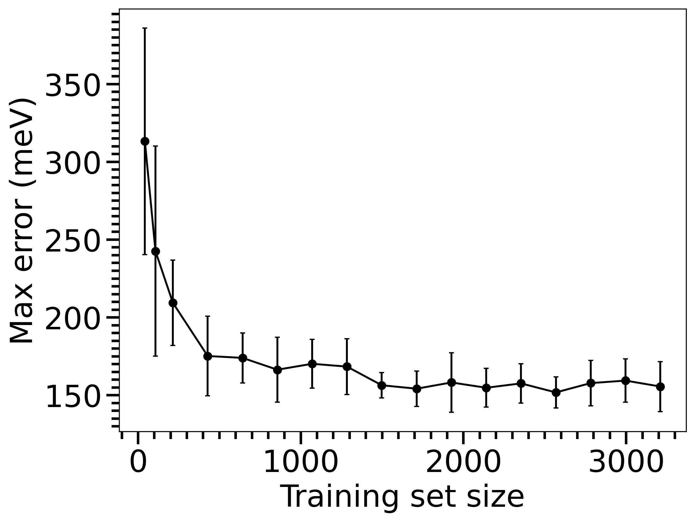
(d)

Figure S3: Dependence of bandgap magnitude prediction (a) RMSE, (b) R², (c) MAE, and (d) Max error from SVR-RBF model on the number of training data. Error bars show standard deviations for 5 trials. The hyperparameters are optimized with RMSE metric.

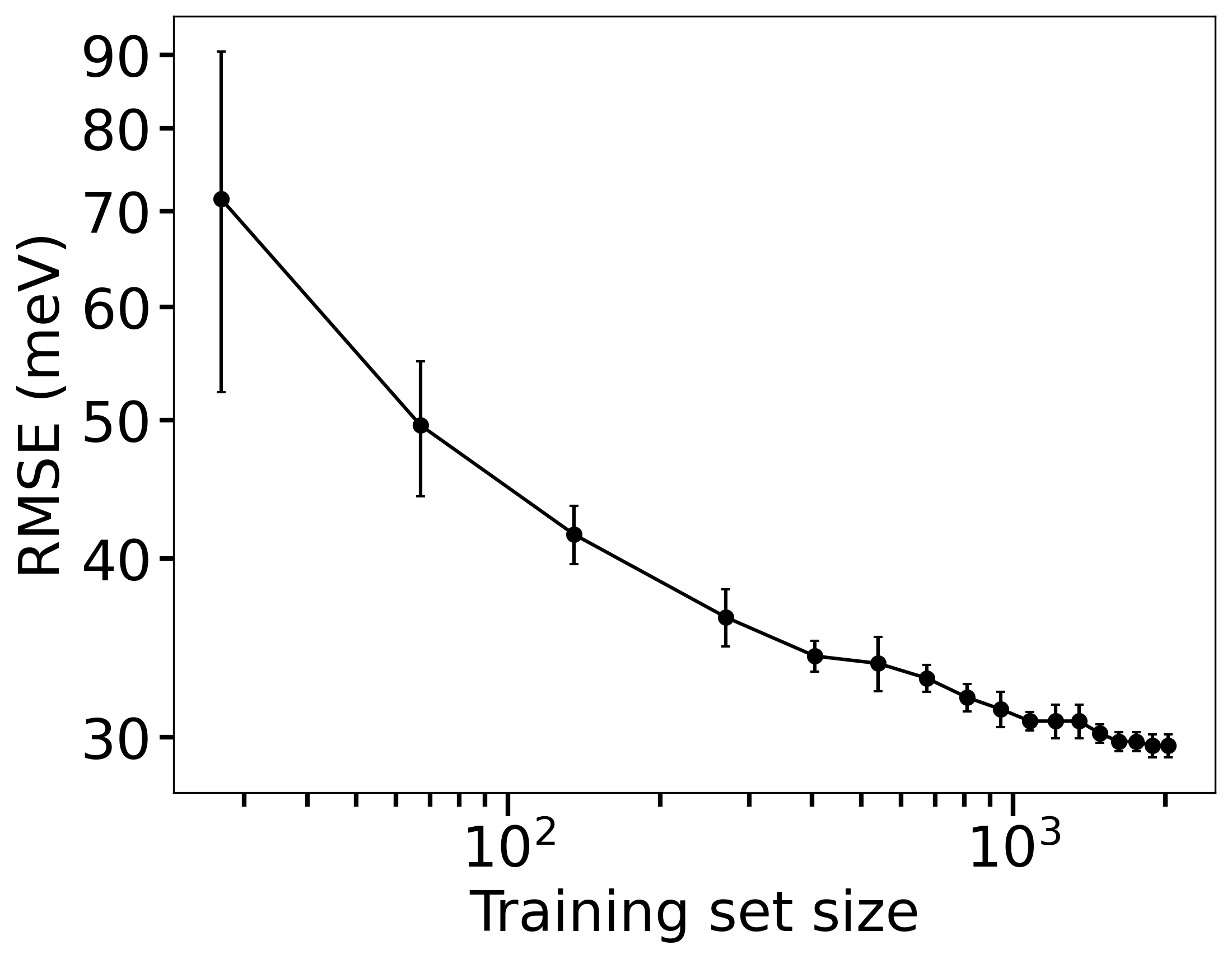
(a)

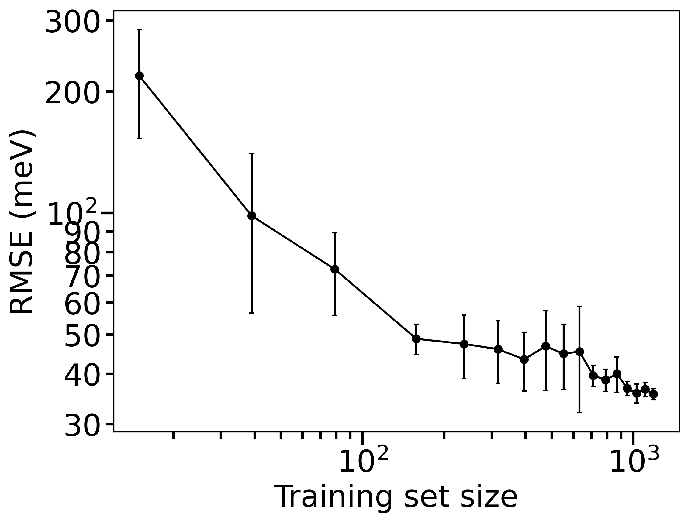
(b)

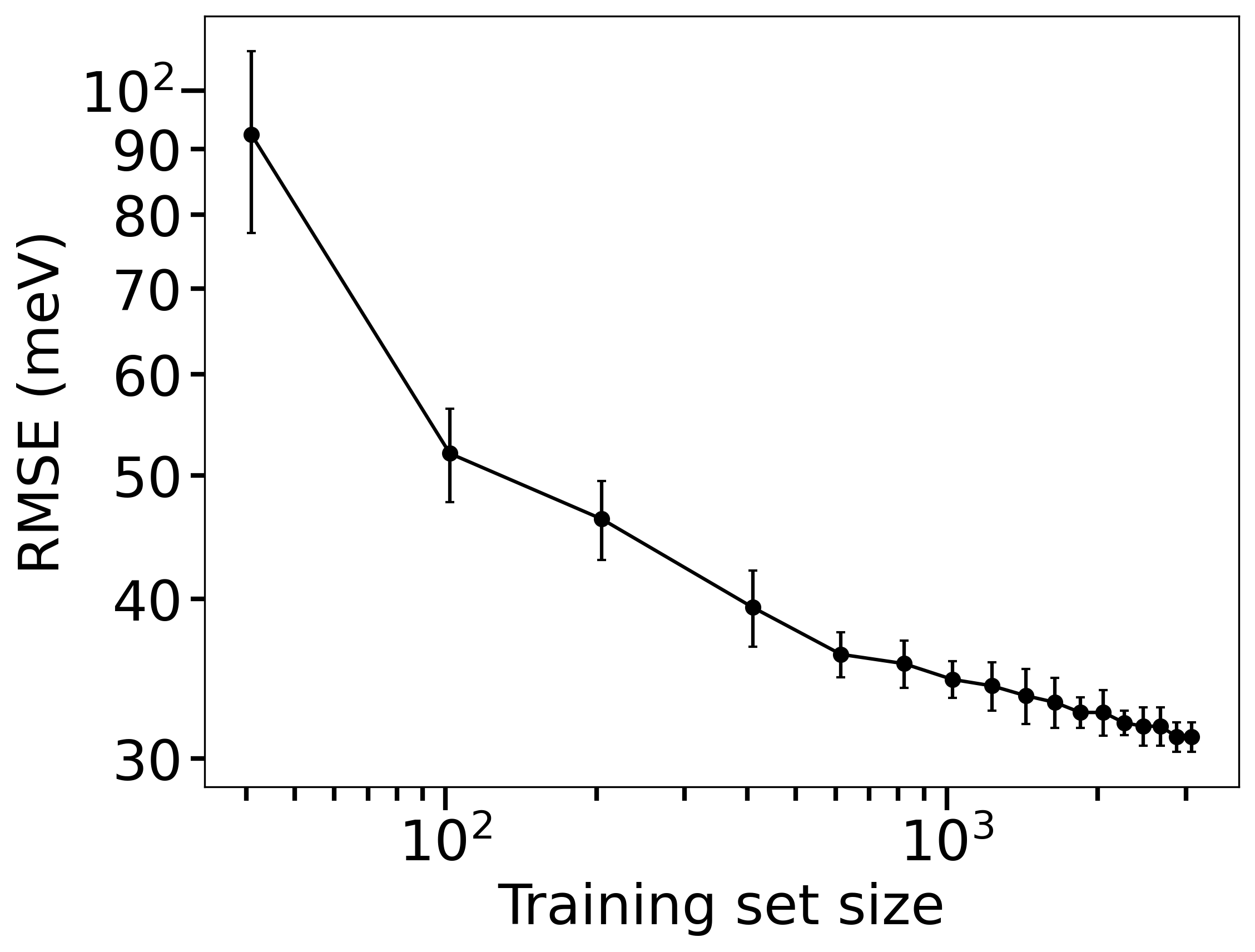
(c)

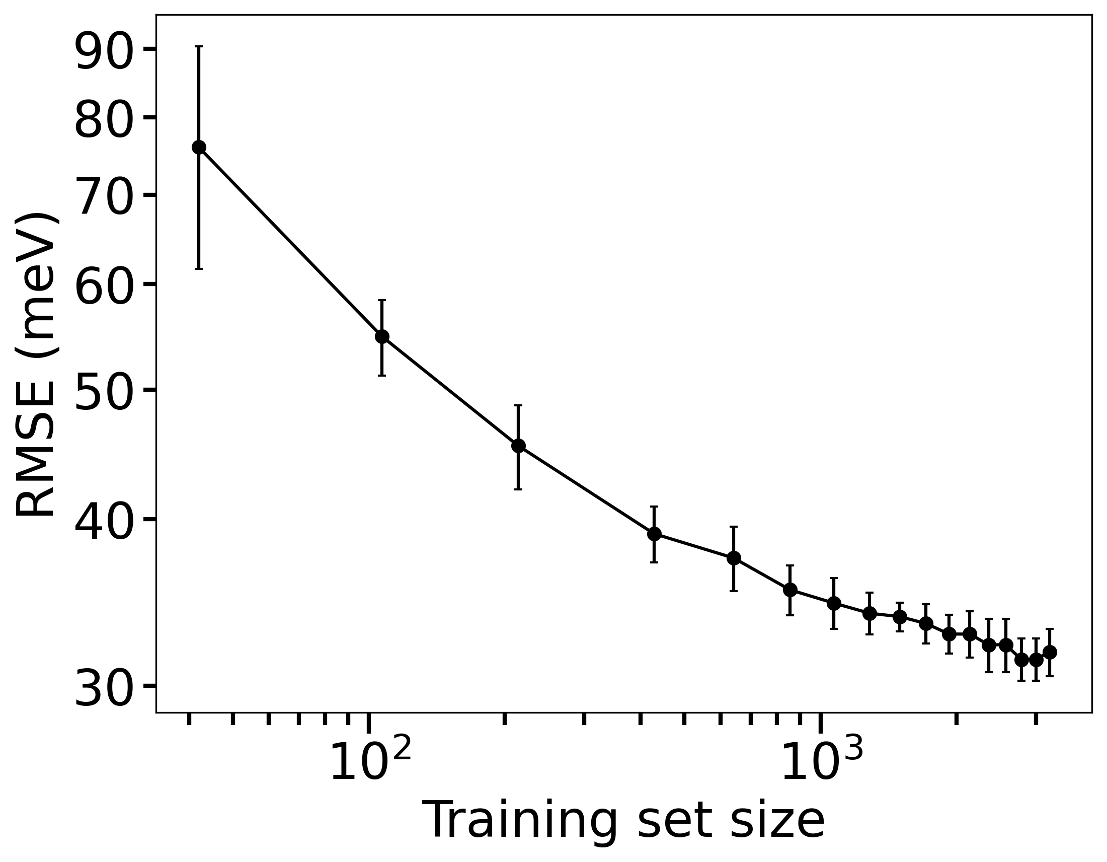
(d)

Figure S4: Learning curve in log–log scale showing the performance of the SVR-RBF model for bandgap value predictions, with different dataset settings: (a) using the dataset that contains only direct bandgaps, (b) using the dataset that contains only indirect bandgaps, (c) using the dataset that contains both direct and indirect bandgaps while excluding the data points for which SVC-RBF model predicted an incorrect bandgap nature, and (d) using the original dataset. Figure (d) corresponds to Fig. 1a in the main manuscript. Error bars show standard deviations over 5 trials. The hyperparameters are optimized with RMSE metric.

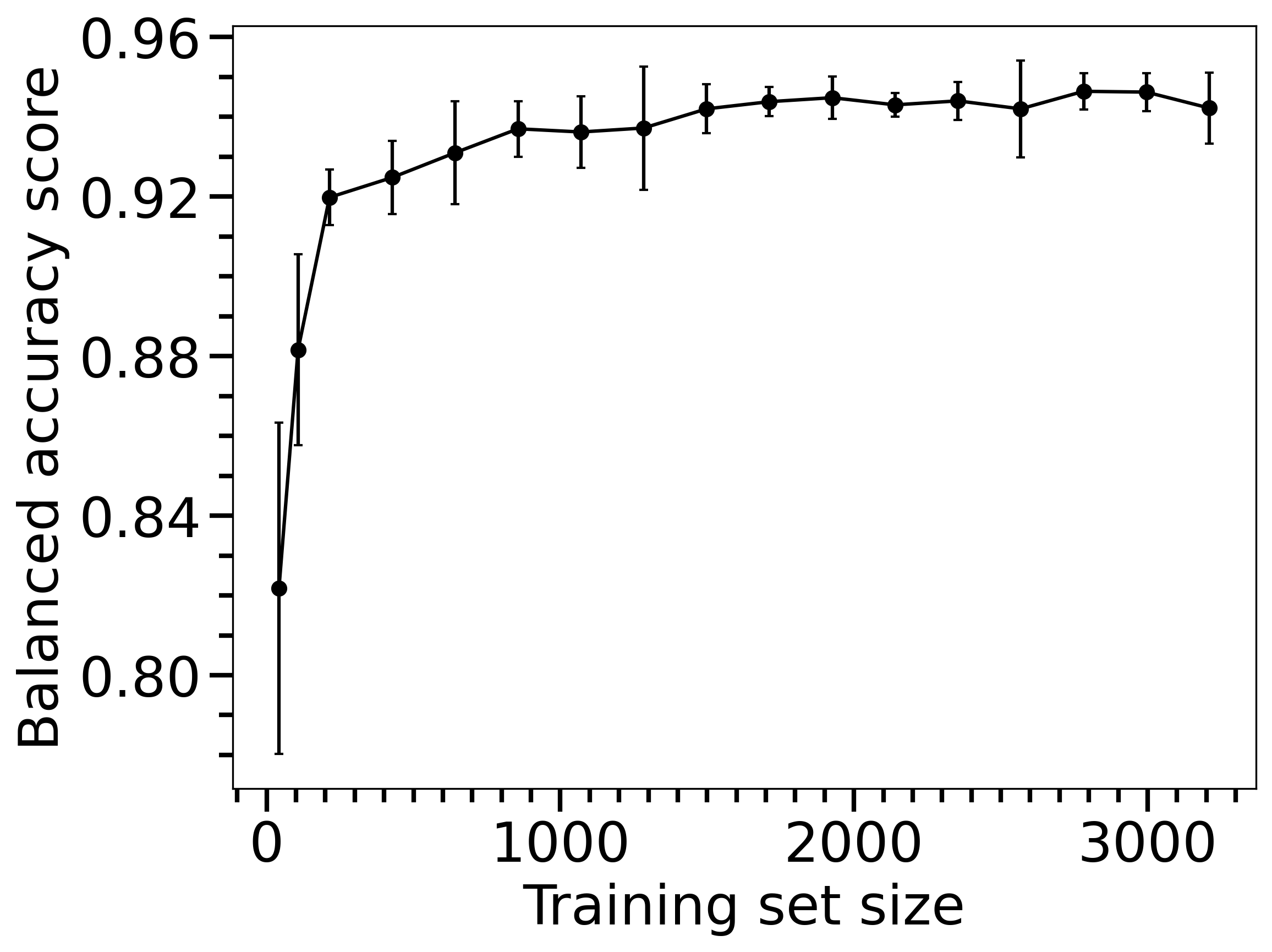
Figure S5: Dependence of bandgap nature prediction balanced-accuracy-score from SVC-RBF model on the number of training data. Error bars show standard deviations for 5 trials. Hyperparameters are optimized with accuracy-score metric.

S5.   Bandgap prediction validations

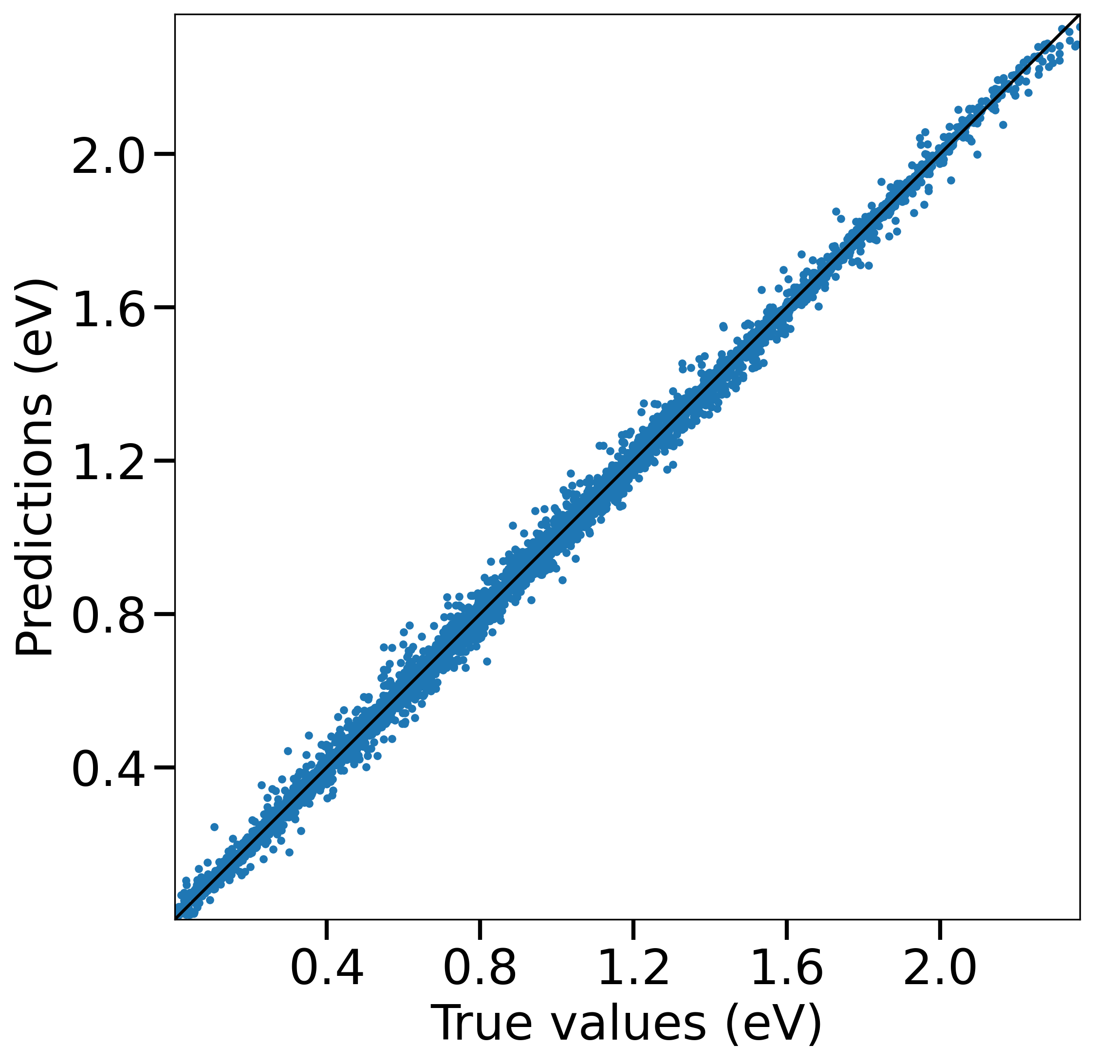
(a)

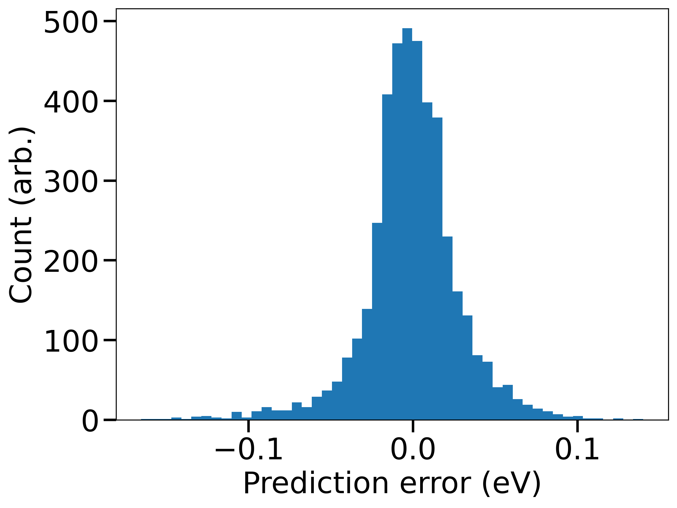
(b)

Figure S6: The bandgap values prediction from the SVR-RBF models for all input data in the dataset. True values are the DFT calculated bandgap values. The predictions are the average bandgap values over the 5 model predictions from the trial set of the last point from Fig. 1a. (a) shows the comparison between true and predicted values, (b) is the prediction error (true value minus predicted value) distribution.

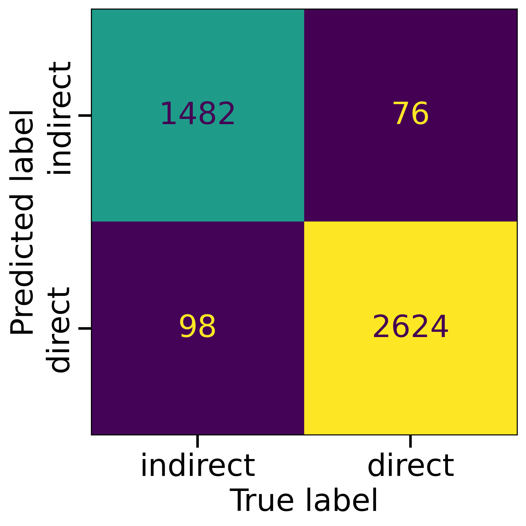
Figure S7: The confusion matrix of the bandgap nature predictions, showing the number of correct and wrong predictions for each class (direct and indirect). True labels are the bandgap nature determined from DFT calculations for all input data in the dataset. The prediction labels are the most frequent outcomes over the 5 SVC-RBF model predictions (mode value) from the trial set of the last point from Fig. 1b.

S6.   Standard deviation distribution of bandgap prediction

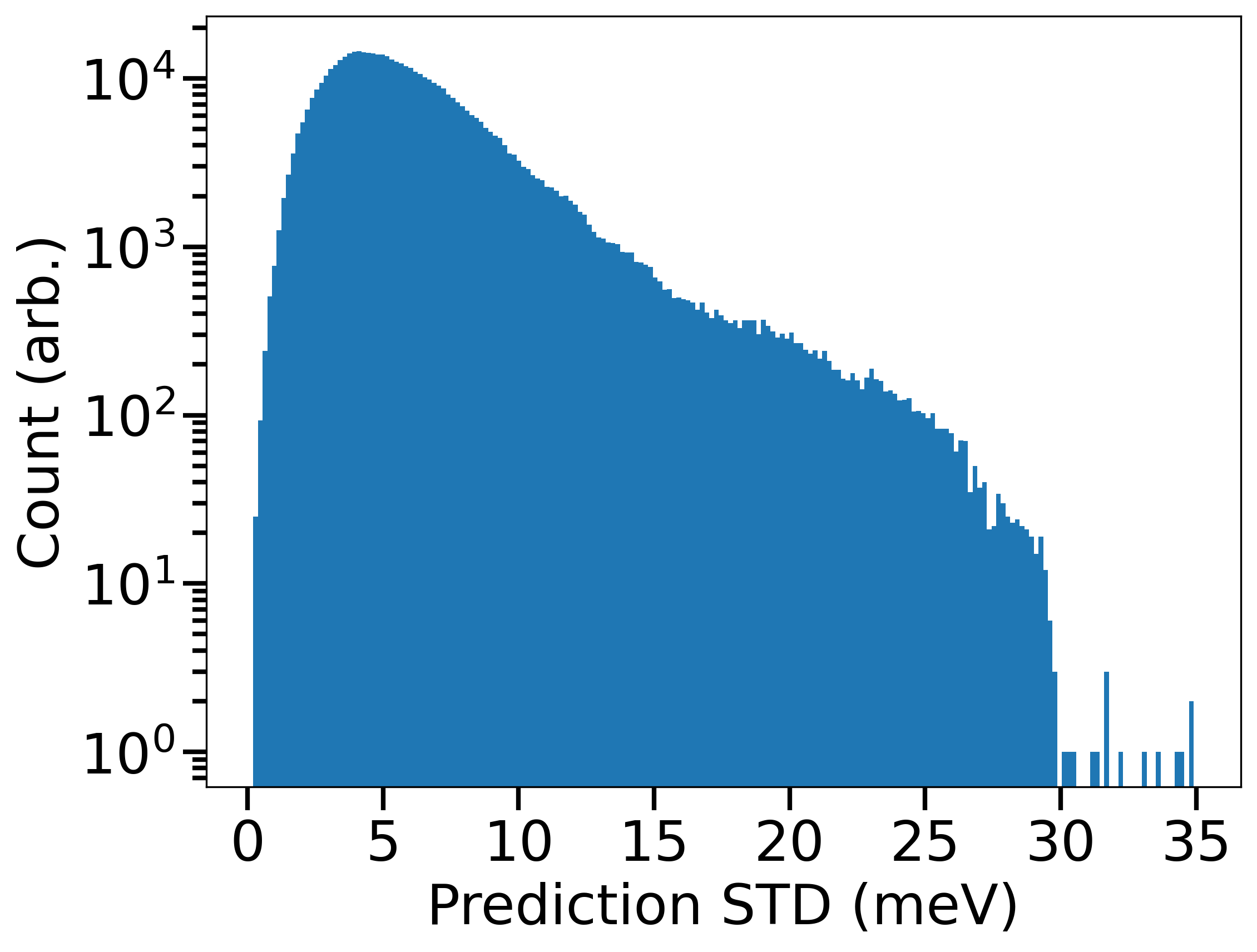
Figure S8: The standard deviation (STD) distribution of bandgap value predictions using the 5 SVR-RBF models from the last point of Fig. 1a. The figure is plotted in semi-log scale.

S7.   Smoothening direct-indirect transition line

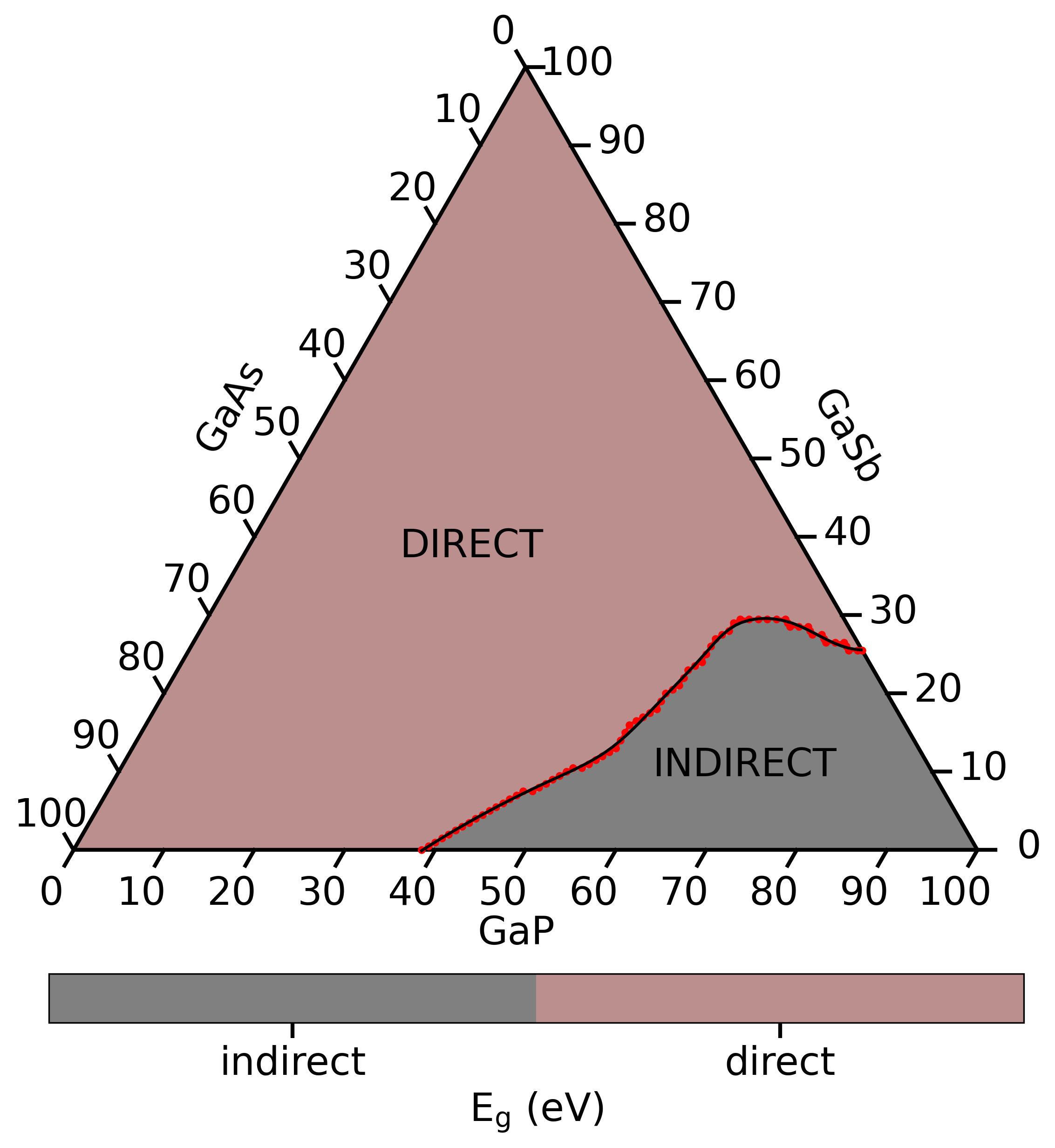
Figure S9: The mapping of bandgap nature for unstrained GaAsPSb (0.0% strain). The labels ‘direct’ and ‘indirect’ describe the enclosed regions, with the nature of bandgap being direct and indirect, respectively. These areas are separated by the direct-indirect transition (DIT) points (red dots). The bandgap natures calculated are the most frequent outcomes over the 5 predictions (mode value) from the trial set of the last point from Fig. 1b. The calculated DIT points (red dots) are fitted (black line) with B-spline function with the smoothing factor, s=5.

We smoothen the calculated discrete direct-indirect transition (DIT) points with B-spline function [1] (smoothing factor, s=5) as is implemented in scipy.interpolated [2] routine.

from scipy.interpolate import splprep, splev
x = DIT_x #x-coordinate of the calculated DITs
y = DIT_y #y-coordinate of the calculated DITs
tck, u = splprep([x, y], s=5)
smoothen_DIT_x, smoothen_DIT_y = splev(u, tck)

S8.   Bandgap values variation under strain for specific GaAsPSb

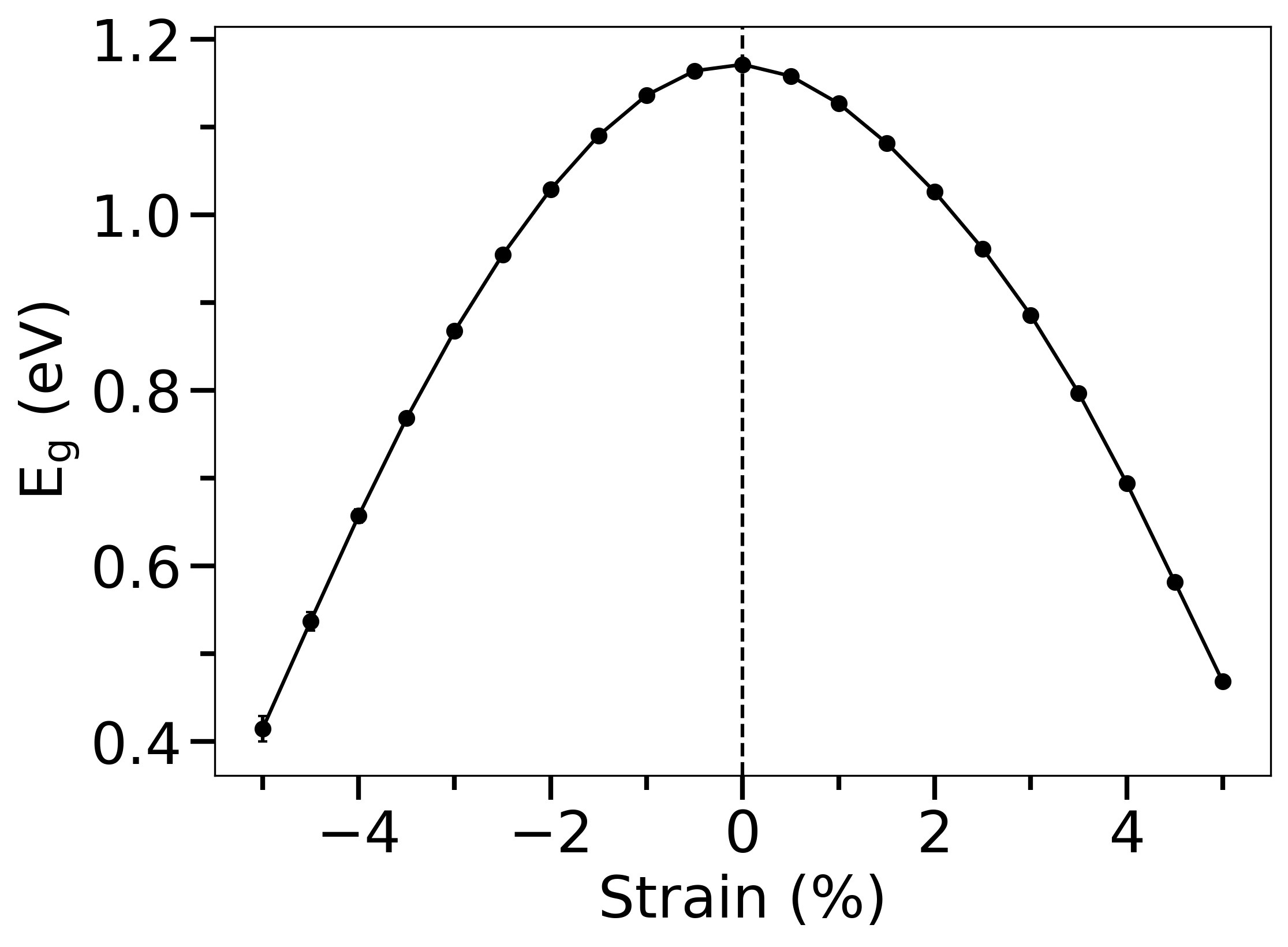
Figure S10: The variation of bandgap values (E${}_{\text{g}}$) under biaxial strain in GaAs_0.333P_0.333Sb_0.334. The positive and negative strain values indicate the tensile and compressive strains, respectively. The bandgap values are the average values over the 5 model predictions from the trial set of the last point from Fig. 1a and error bars show standard deviations.

S9.   Substrate effect in GaAsPSb bandgap phase diagram

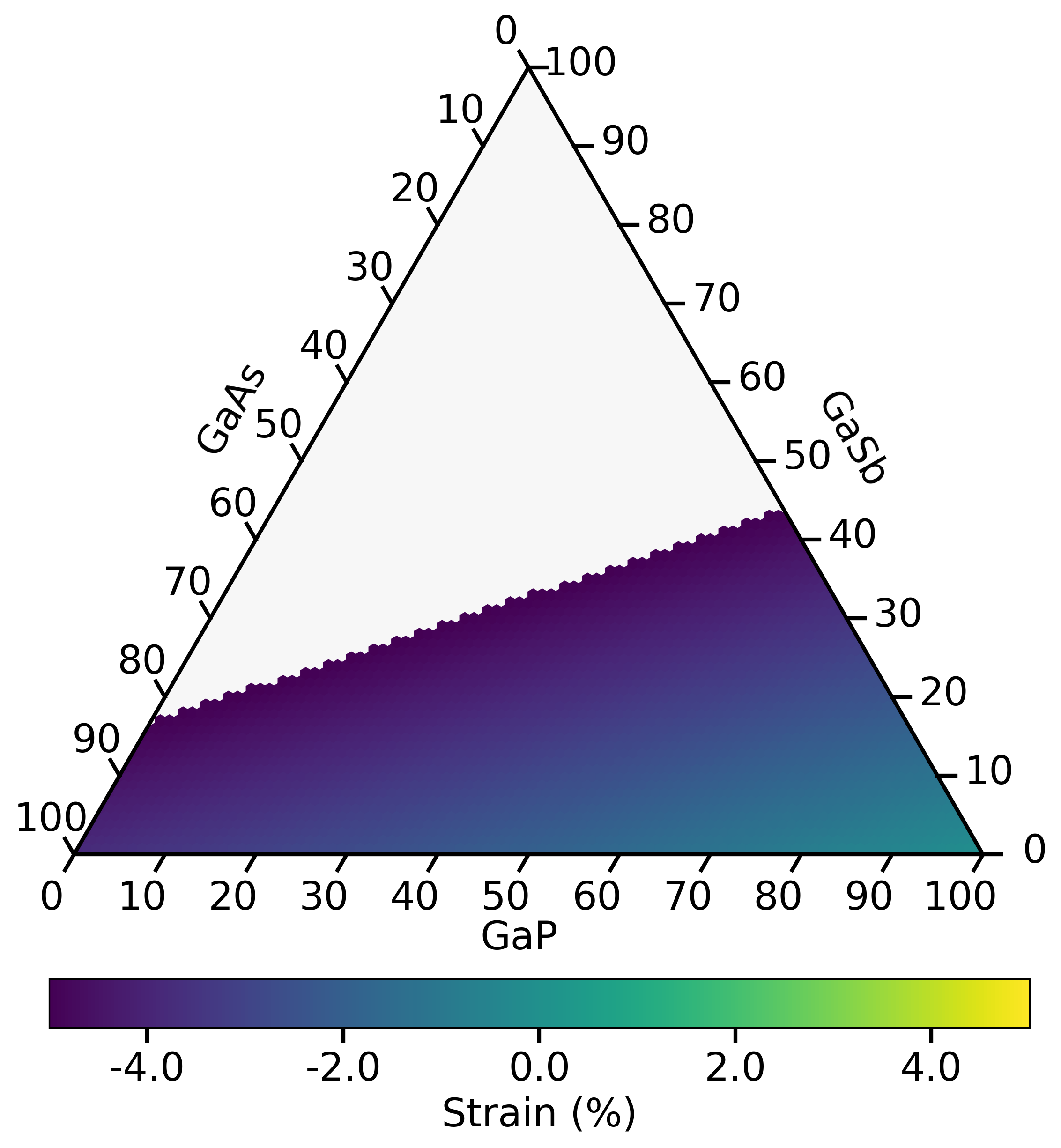
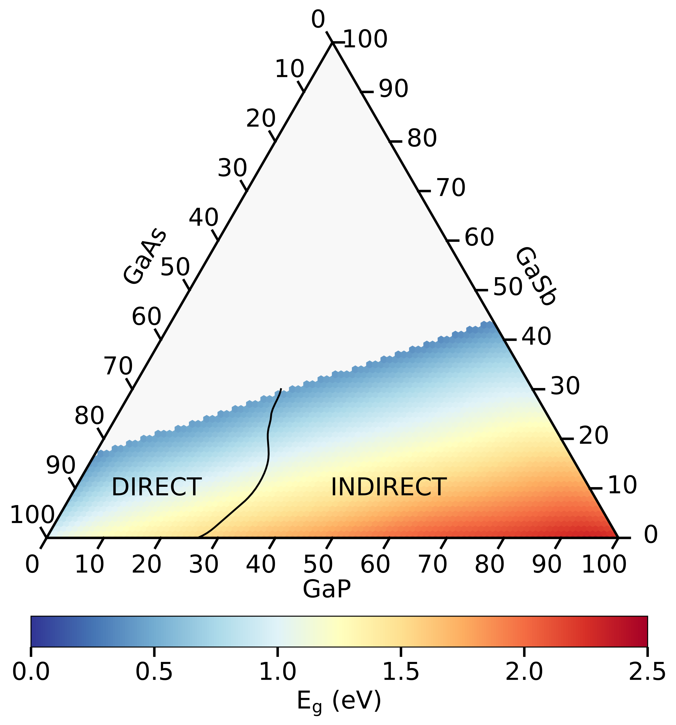
(a) GaP substrate

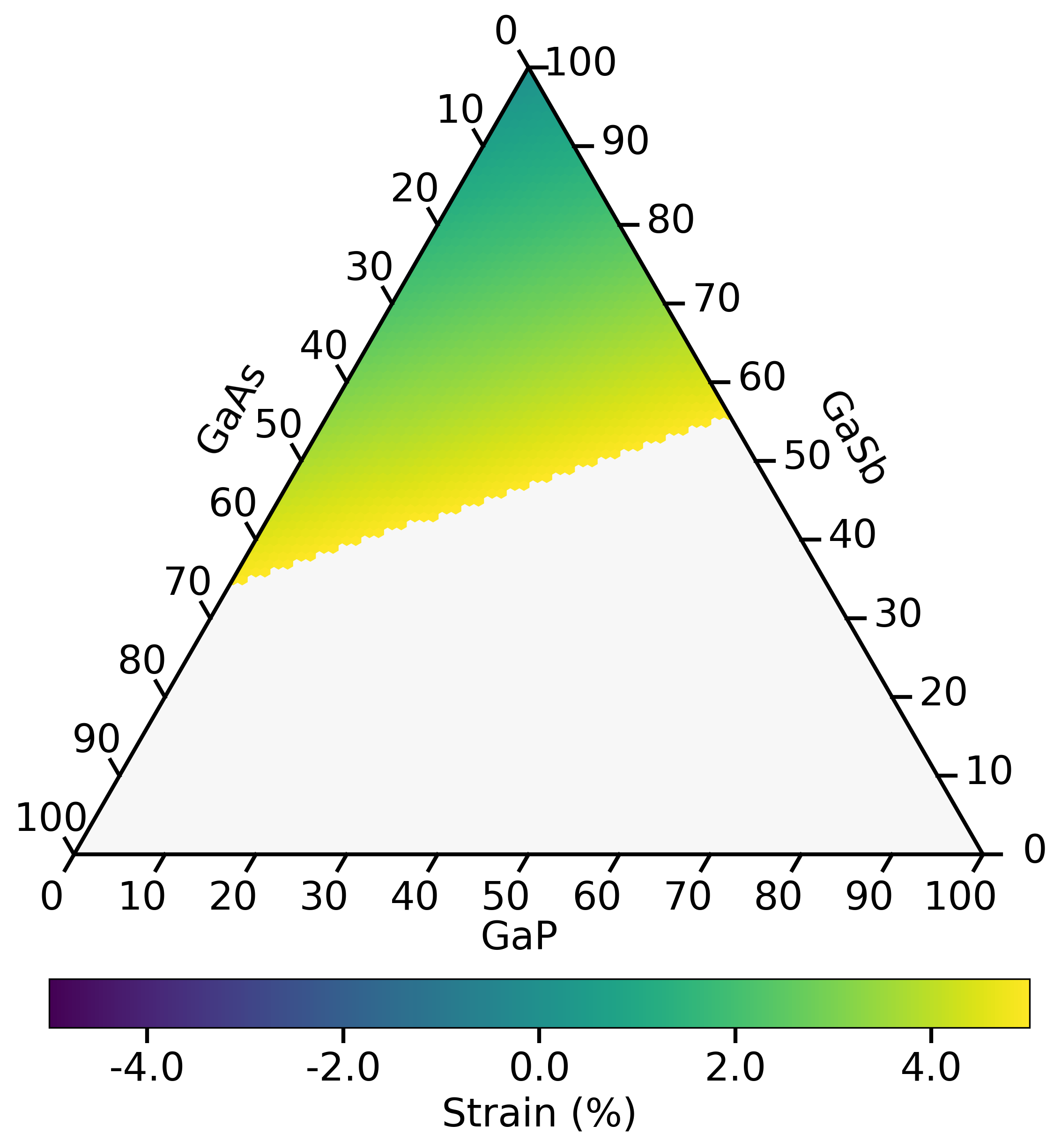
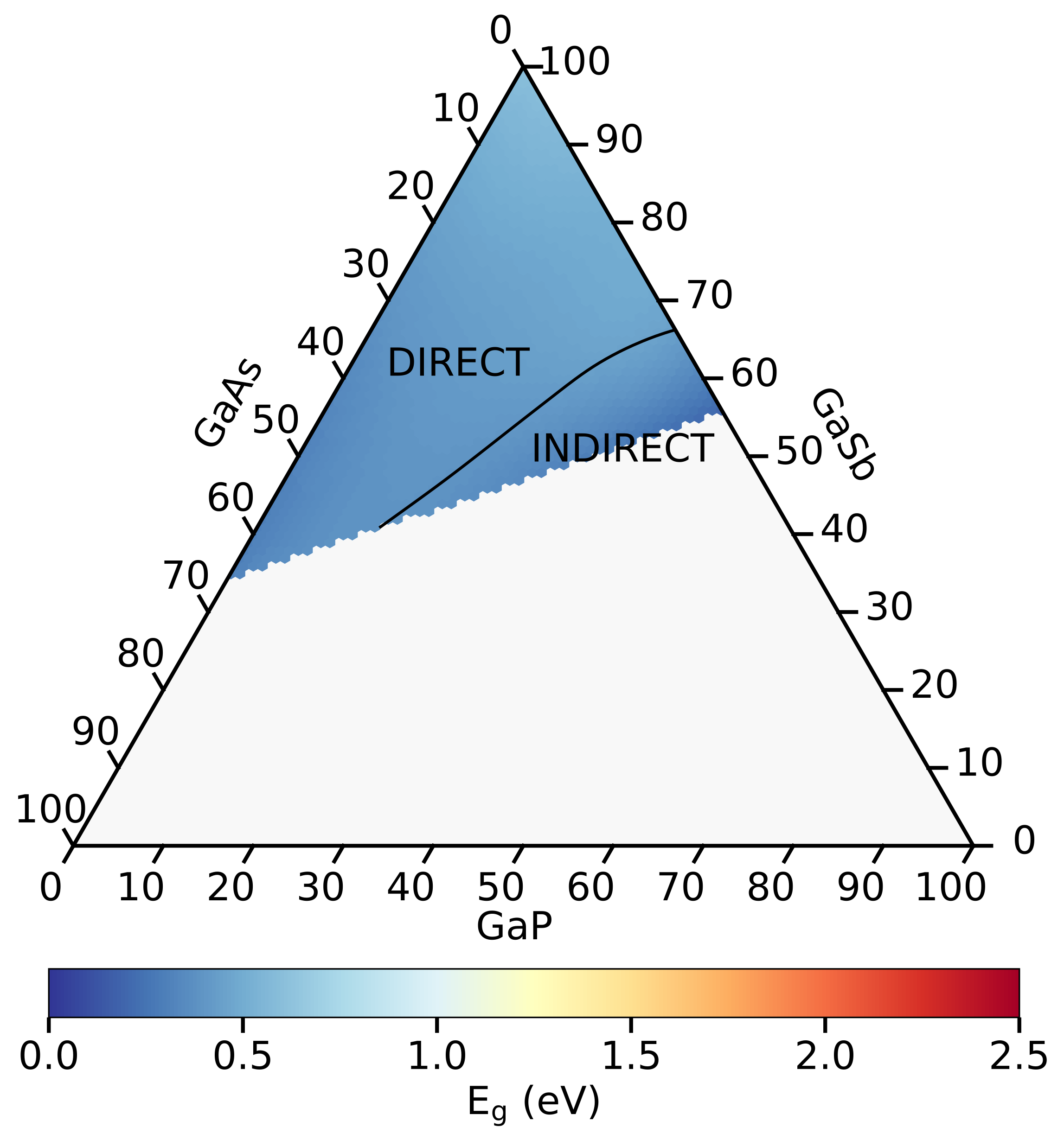
(b) GaSb substrate

Figure S11: The effect of substrate on GaAsPSb epi-layer under the ‘theoretical epitaxy’ model [3, 4] (up to $5\%$ compressive and tensile strain). The left column shows the calculated biaxial strain values using Eqs. 8 and 9. The right column presents predicted bandgap values in color (E${}_{\text{g}}$). The labels ‘direct’ and ‘indirect’ describe the enclosed regions, with the nature of bandgap being direct and indirect, respectively. The bandgap values are the average values over the 5 model predictions from the trial set of the last point from Fig. 1a. The nature of the bandgaps are the most frequent outcomes over the 5 predictions (mode value) from the trial set of the last point from Fig. 1b.

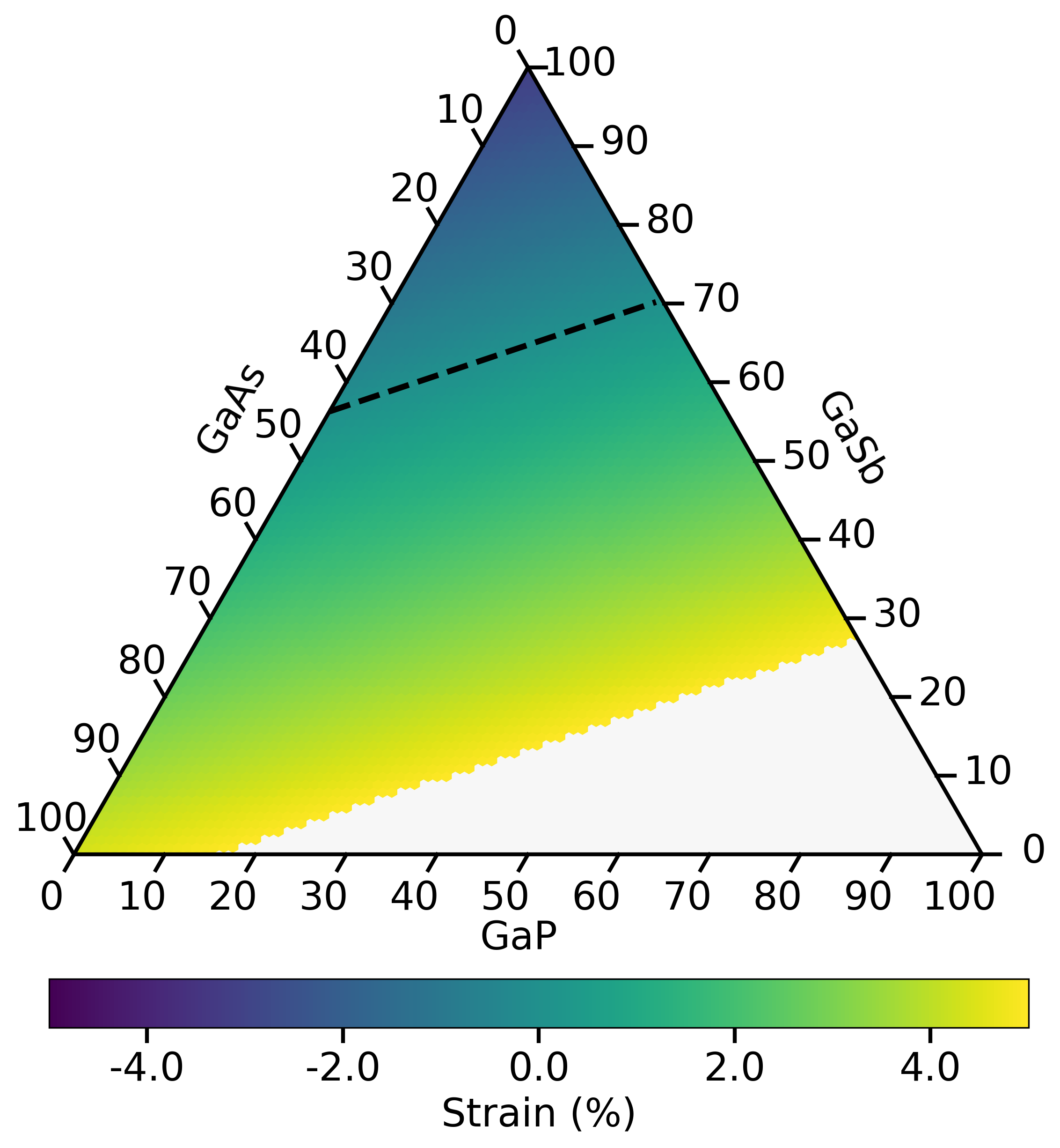
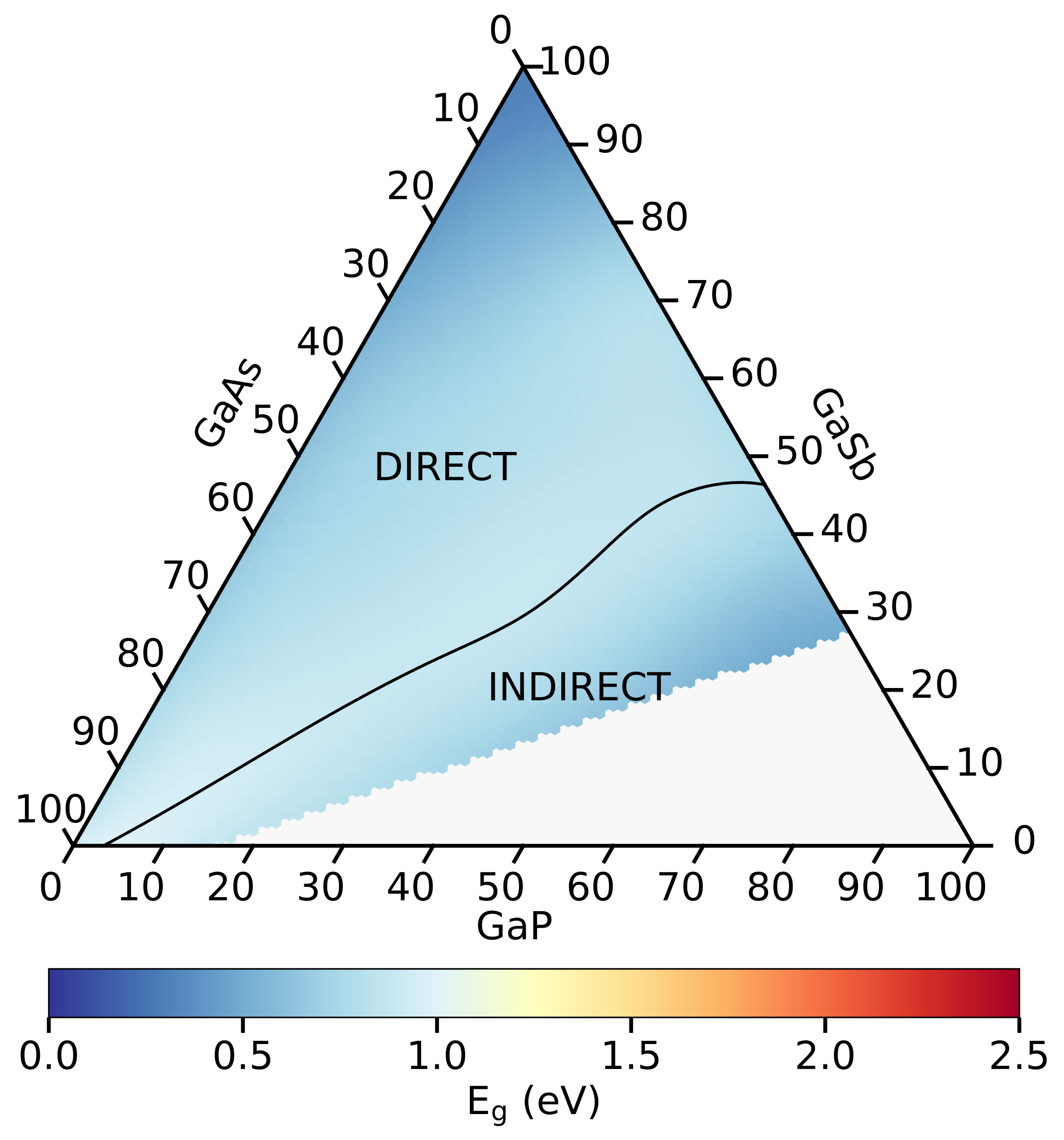
(c) InP substrate

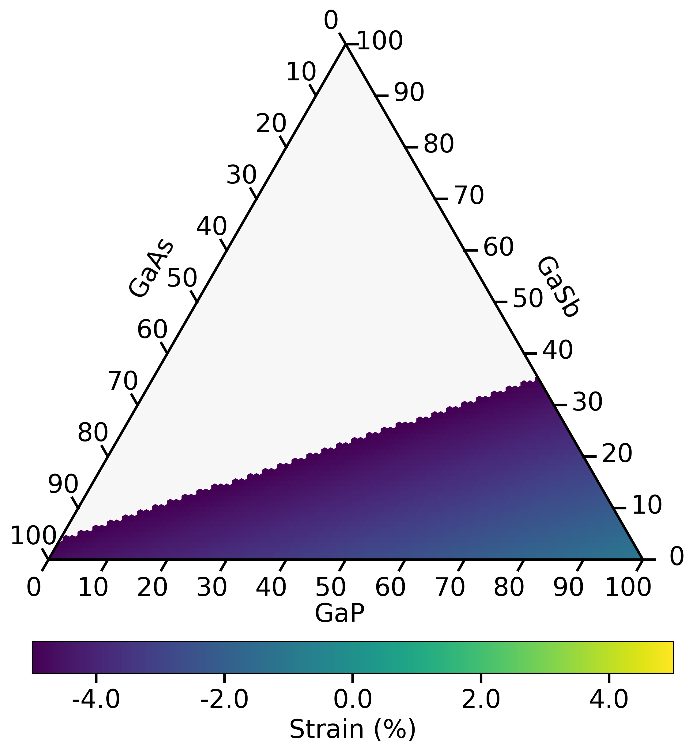
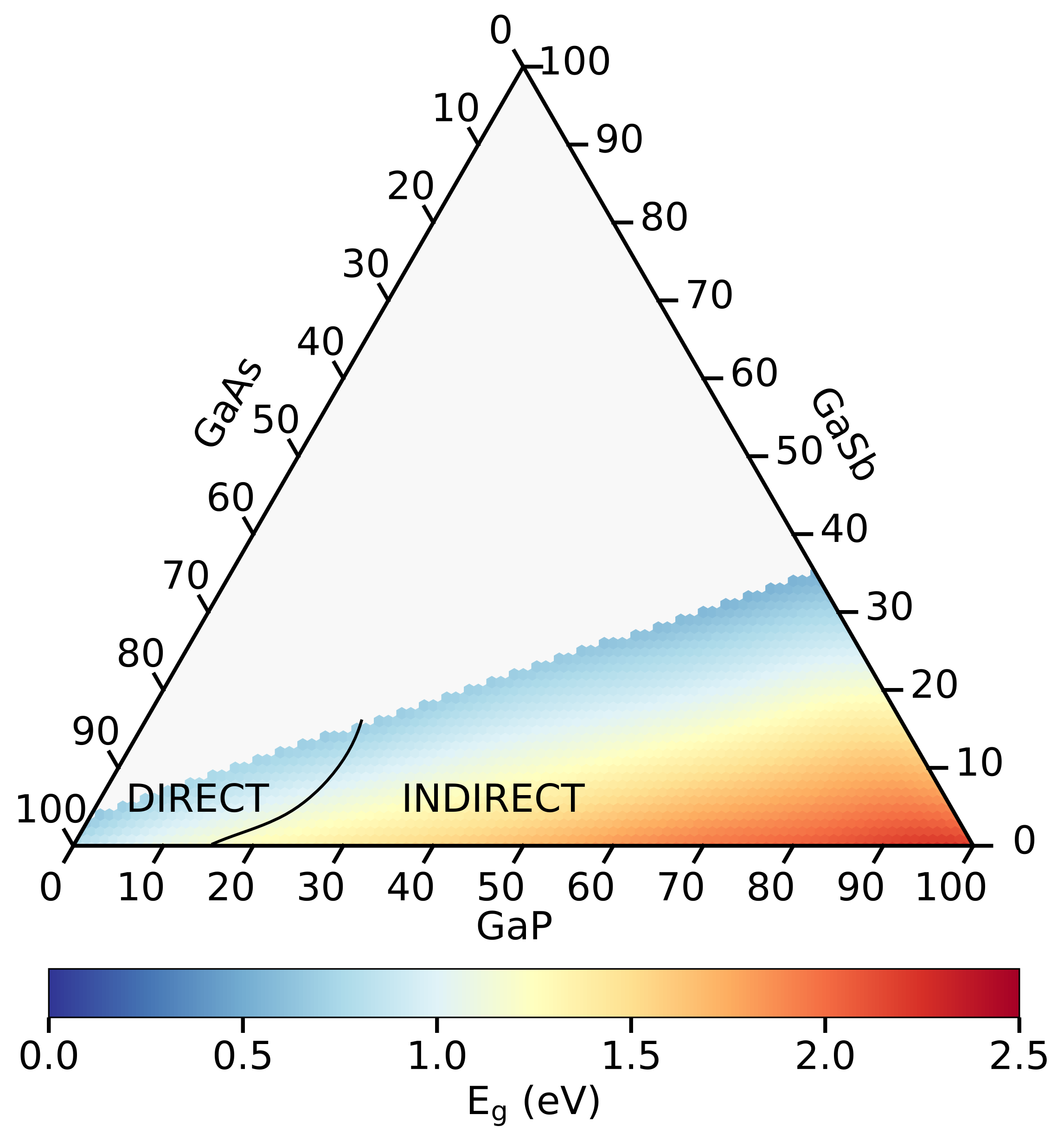
(d) Si substrate

Figure S11: (continue) The effect of substrate on GaAsPSb epi-layer under the ‘theoretical epitaxy’ model [3, 4] (up to $5\%$ compressive and tensile strain). The left column shows the calculated biaxial strain values using Eqs. 8 and 9. The black dotted line in (c) indicates the perfect lattice matching (no strain) compositions. The right column presents predicted bandgap values in color (E${}_{\text{g}}$). The labels ‘direct’ and ‘indirect’ describe the enclosed regions, with the nature of bandgap being direct and indirect, respectively. The bandgap values are the average values over the 5 model predictions from the trial set of the last point from Fig. 1a. The nature of the bandgaps are the most frequent outcomes over the 5 predictions (mode value) from the trial set of the last point from Fig. 1b.

References

• Dierckx [1982] P. Dierckx, Algorithms for smoothing data with periodic and parametric splines, Comput. Graph. Image Process. 20, 171 (1982).
• P. Virtanen et al. [2020] P. Virtanen et al., SciPy 1.0: fundamental algorithms for scientific computing in Python, Nat. Methods 17, 261 (2020).
• Mondal and Tonner-Zech [2023] B. Mondal and R. Tonner-Zech, Systematic strain-induced bandgap tuning in binary III-V semiconductors from density functional theory, Phys. Scr. 98, 065924 (2023).
• Mondal et al. [2023] B. Mondal, M. Kröner, T. Hepp, K. Volz, and R. Tonner-Zech, Accurate first principles band gap predictions in strain engineered ternary III-V semiconductors, Phys. Rev. B 108, 035202 (2023).