On the use of ordered factors as explanatory variables

The present version of the paper essentially coincides with the one appearing in Stat 12, e624 (2023), freely accessible at https://doi.org/10.1002/sta4.624. The only difference is in the very last paragraph of the main body of the text.

Abstract Consider a regression or some regression-type model for a certain response variable where the linear predictor includes an ordered factor among the explanatory variables. The inclusion of a factor of this type can take place is a few different ways, discussed in the pertaining literature. The present contribution proposes a different way of tackling this problem, by constructing a numeric variable in an alternative way with respect to the current methodology. The proposed techniques appears to retain the data fitting capability of the existing methodology, but with a simpler interpretation of the model components.

1 Context and aim

The statistical analysis of data arising from categorical variables, or factors, of ordered type involves specialized techniques. A valuable general treatment of the pertaining methods is provided by Agresti, (2010). To introduce notation, denote by $X$ the ordered factor under consideration, whose levels $1,\dots,K$ are in increasing order in some recognized sense, but they do not represent values on a numerical scale. For the study of relationship among a set of variables, the situation more extensively discussed in the specialized literature refers to the case where $X$ represents the response variable.

The present note deals instead with a different situation, namely with the case where $X$ plays the role of an explanatory variable, not the response one. This other setting has received substantially less attention in the literature. After a brief survey of the existing options for making use of $X$ as an explanatory variable in a linear model or a generalized linear model, we shall put forward a new proposal.

The inclusion of an ordered factor in a linear predictor implies its transformation into some numeric variable, or possibly a number of them. For the selection of a suitable numerical score scheme to be used as an explanatory variable, Armitage, (1955) and Graubard & Korn, (1987) provide essentially similar recommendations, as follows: (i) the ideal route is to identify some numerical score with a convincing subject-matter interpretation; (ii) in the absence of any a priori knowledge towards such a choice, one must pick-up some numeric values, and equally spaced values are the natural option to consider, at least as the initial choice. Since route (ii) involves a subjective choice, it has generated much debate over the years, and still it does, as demonstrated for instance by the views presented fairly recently by Pasta, (2009) and Williams, (2020).

In the common case that one chooses to employ equally spaced values as scores, it is however appropriate to test the assumption of linearity of the effect. For instance, Section 2 of Armitage, (1955) presents a decomposition of the variability due to $X$ into two components, the one due to linearity and the one due to departure from linearity.

Moving further in this direction, one can introduce more than one numeric variable. A specific option is to consider a sequence of orthogonal polynomials evaluated at $(1,\dots,K)$ or at an affine transformation of this sequence, so that the total variability associated to $X$ can be decomposed into components associated to the linear, quadratic, and other polynomial terms, with components up to a maximal degree $K-1$. An early exemplification of this procedure is provided by Winer, (1962, pp. 70–77), in a numerical illustration involving the effect of a six-level factor representing ‘complexity’ of a certain visual display, whose effect is decomposed into linear, quadratic, cubic and residual components.

This logic is currently standard practice. Specifically, in the R computing environment (R Core Team,, 2022), ordered factors are handled in this way unless an alternative choice is explicitly made; see the documentation of command contr.poly for details. This strategy is in line with the indications of Chambers & Hastie, (1993, p. 32) who prescribed that “ordered factors are coded so that individual coefficients represent orthogonal polynomials if the levels of the factor were actually equally spaced numeric values”.

However, alternative directions are possible. Specifically, Gertheiss & Tutz, (2009) and Tutz & Gertheiss, (2016) have proposed to consider regularization methods for the parameters based on “a penalty which enforces that estimates of coefficients for adjacent categories are not too far apart”. This is a way of approaching the problem which, as highlighted by the discussion in Gertheiss & Tutz, (2009, pp. 347–8), follows a different logic from the alternative of assigning scores, as we do here.

While an adequate fit to the data remains a basic requirement for any candidate formulation, the key feature of the present proposal is a simplification of the modelling process via a method which delivers a scoring system. The construction of a scoring system appears to be a desirable feature for many applied researchers, since it typically simplifies interpretation; this aspect will be illustrated in the practical situations presented later. This feature makes a qualitative difference with a number of other proposals, such as those based on regularization methods recalled in the previous paragraph, but also with other formulations. In this view, a numerical comparison with alternative methods beyond the standard ones does not seem to be crucial.

For the sake of completeness, we mention the connection with the paper by Winship & Mare, (1984). However, for ordinal independent variables, they consider a somewhat different setting, namely the case where ordered variables occur as “independent or intervening variables in structural equation models”.

The rest of this note is dedicated to a alternative way of constructing a set of scores, where the basic values $1,\dots,K$ are replaced by a set of not equally-spaced values. The method works by choosing the non-equally-spaced values in place of quadratic or higher-degree polynomial values, with the conceptual advantage of providing numeric scores which reflect the actual data behaviour. The overall aim is to construct a numeric response variable which replaces the original ordered factor, retaining a similar fitting ability but allowing a simpler interpretation. The procedure is illustrated by two numerical exemplifications, followed by a set of concluding remarks.

2 A method for choosing scores

2.1 The rationale of the formulation

The basic scores $1,\dots,K$ are equivalent to the scaled values $u_{k}=k/(K+1)\in(0,1)$ for $k=1,\dots,K$. In case the original scores span a different set of values, such as $0,1,\dots,K-1$, there exists some other affine transformation to achieve the same $u_{k}$’s values; the only requirement is that the original scores are equally spaced. Our aim is to select a non-linear transformation of the $u_{k}$’s, which can better fit the data pattern than the equally-spaced scores. This plan can be broadly viewed as a replacement of the above-mentioned suggestion by Armitage, (1955) and Graubard & Korn, (1987) of identifying scores with subject-matter interpretation, in the frequently occurring cases where a specification with such an ideal genesis is not feasible.

Take now into consideration two simple facts: (a) the $u_{k}$’s correspond to a set of equally-spaced quantiles of the $U(0,1)$ distribution, and (b) the transformation of these values must be monotonically increasing. For simplicity of treatment, we shall focus on the case where monotonicity holds in a strict sense, although this is not logically compelling; on this point, see also the final paragraph of Section 2.2. Combining remarks (a) and (b), we are led to consider transformations of the type $q_{k}=Q(u_{k})$ where $Q$ is a continuous quantile function, that is, the inverse of a continuous distribution function $P=Q^{-1}$. Hence the $q_{k}$’s represent the quantiles of $P$ at the levels $k/(K+1)$, for $k=1,\ldots,K$.

From the formal viewpoint, we have not yet made any progress, since the $q_{k}$’s simply represent an arbitrary sequence of numbers, with only the condition of monotonicity. Their interpretation as quantiles, however, lends itself to the introduction of a flexible parametric family of distributions from which to select a suitable member $P$. We shall sometimes write $q_{k}(\theta)=Q(u_{k};\theta)$ to emphasize the dependence on the parameter vector $\theta\in\mathbb{R}^{p}$ which identifies a given distribution in the parametric family.

It is widely recognized that, at least in the univariate context like the present one, flexible parametric families can be used to approximate closely an arbitrary continuous distribution, except possibly very peculiar situations. Some numerical evidence in this direction has been provided by Solomon & Stephens, (1978) using the Pearson system of curves, but the underlying idea applies more generally. For instance, Hoaglin, (1984) illustrates how the $g$-and-$h$ family can satisfactorily approximate a given target distribution, such as $\chi^{2}_{6}$ and Cauchy; the $g$-and-$h$ family will be recalled later. We shall return to the use of flexible parametric families in a short while.

Before proceeding further, we summarize the essence of the proposal, which is as follows: (i) adopt a flexible parametric family of continuous distributions; (ii) select its member $P$ whose quantile values $q_{k}$’s are most effective at fitting the data under consideration, and denote these quantiles by $q_{k}(\hat{\theta})$; (iii) optionally, these $q_{k}(\hat{\theta})$ are transformed on the original scale to produce new working scores, for instance adopting $(K{+}1)\,q_{k}(\hat{\theta})$ as the final scores. In next subsection, we discuss the more operational side of steps (i) and (ii).

2.2 On the choice of the transformation

To start with, the methodology requires to select a flexible parametric family of univariate continuous distributions. We discuss some guidelines for its choice.

Unless the specific problem under consideration incorporates some features which indicate differently, it is appropriate to work with distributions having support on the entire real line, to avoid unnecessary restrictions on the $q_{k}$’s. Typically, such distributions include parameters for the regulation of location, scale and shape, with shape often regulated by more than one parameter. For our purposes, however, location and scale can be fixed at 0 and 1, say, since their effect can be subsumed under the other components of the (generalized) regression model. Hence, we are only interested in regulating the shape parameters, of which there are typically two.

Even with these considerations, the choice is among a vast set of options. Consider that the fitting process involves the computation of $Q(u_{k};\theta)$ for all values of $k$ and for many candidate $\theta$’s. From the computational viewpoint, it is then advantageous to work with a family of distributions whose quantile function can be computed efficiently, ideally via an explicit expression.

Along this line of thinking, a convenient setting is represented by families obtained from transformations of the normal distribution. A classical construction of this type is the $S_{U}$ distribution introduced by Johnson, (1949); the main ingredients are summarized by Johnson et al., (1994, Chapter 12, § 4.3) under the heading ‘Transformed Distributions’. The essence of the construction is as follows: start with a standard normal random variable $Z$ and define $\tilde{Z}=(Z-\gamma)/\delta$ for given real parameters $(\gamma,\delta)$, where $\delta$ is positive; then an instance $Y$ of the $S_{U}$ family (without inclusion of location and scale parameters) is generated by the transformation

$$Y=\sinh\tilde{Z}=\mbox{$\textstyle\frac{1}{2}$}\left(e^{\tilde{Z}}-e^{-\tilde{Z}}\right).$$ (1)

As the parameters $(\gamma,\delta)$ span their admissible range, the $S_{U}$ family exhibits a high degree of flexibility. In particular, the measures of skewness and kurtosis vary considerably. If $\gamma=0$, the density of $Y$ is symmetric about 0.

Another construction of similar logic is represented by the Tukey $g$-and-$h$ distribution, discussed in detail by Hoaglin, (1984). Also in this case, we start from the random variable $Z$ as before, but its transformation takes now the form

$$Y=\cases{Z\>e^{h\,Z^{2}/2}&\hbox{if\leavevmode\nobreak\ } g=0,\cr g^{-1}\left(e^{g\,Z}-1\right)e^{h\,Z^{2}/2}&\hbox{otherwise}}$$ (2)

for arbitrary parameters $g$ and $h$, provided $h\geq 0$. Also for the $g$-and-$h$ distribution, the measures of skewness and kurtosis span a considerable range. If $g=0$, the density of $Y$ is symmetric about 0. If both $g=0$ and $h=0$, 2 reduces to $Y=Z$.

Yet another construction is the $\mathrm{sinh}$–$\mathrm{arcsinh}$ distribution introduced more recently by Jones & Pewsey, (2009). This is based on the transformation

$$Y=\sinh\left(\frac{\mathrm{arcsinh}\,Z+\varepsilon}{\delta}\right)$$ (3)

where $\varepsilon$ is a real-valued parameter which regulates skewness, with sign in agreement with the one of $\varepsilon$, and $\delta$ is a positive parameter which regulates tailweight. When $\varepsilon=0$ and $\delta=1$, 3 reduces to $Y=Z$. A convenient feature of 3 is that it can generate both lighter tails than the normal (if $\delta>1$) and heavier ones (if $\delta<1$).

While the $S_{U}$, the $g$-and-$h$ and the $\mathrm{sinh}$–$\mathrm{arcsinh}$ families appear to be suitable for our purposes, there is no compelling reason for their choice. In specific problems, other families of distributions could possibly be preferable.

A reviewer of this paper has suggested considering the Beta family because of its high flexibility as the parameters vary. Use of the Beta distribution had indeed been explored in an early stage of this project, but the outcome was disappointing. The reason of the unsuccess seemed to be linked to the bounded support of the distribution, while the extemal classes of the factors typically call for wide ranges of the quantiles. The issue of restricted range of the distribution cannot be overcome by considering an arbitrary range $(a,b)$, say, instead of $(0,1)$, regarding $(a,b)$ as additional parameters, for the same reason that has excluded the location and scale parameters for the distributions mentioned above.

Another interesting suggestion was to allow that some of the quantiles of $Q$ coincide, so that two or more factor levels could effectively collapse into one, a situation which may be appropriate in some cases. Technically, this extension means removing the condition that $Q$ is strictly monotonic. To achieve this situation, we can consider a transformation distribution obtained as a mixture of a point mass and a continuous distribution. This formulation is interesting, and deserves to be examined in future developments, but for the present presentation we focus on the simpler situation of strictly monotonic transformations, corresponding to preservation of distinct levels of the factor.

3 Numerical illustrations

3.1 Oesophageal cancer data

To demonstrate the working of the method in a concrete situation, we consider a set of data referring to a case-control study of oesophageal cancer reported by Breslow & Day, (1980), and available in the R computing environment as dataset esoph. The aim of the exercise is to model the number of cases and controls using three numerical explanatory variables which have been grouped into categories, hence yielding three ordered factors. Specifically, there are six groups for age (factor agegp), four groups for alcohol consumption (alcgp), and four groups for tobacco consumption (tobgp).

Logistic regression models have been fitted to the number of cases and controls, via the R command glm, with a linear predictor built from the above-described explanatory variables. After fitting an initial model with maximal degrees of the orthogonal polynomials representing the ordered factors, the non-significant components have been removed, leading to the model summarized in Table 1. Here and in the following, the suffixes ‘.L’, ‘.Q’ and ‘.C’ denote the linear, quadratic and cubic terms of a factor. Although the quadratic component of alcgp is not significant, it has been retained because the cubic component is, in order to follow a hierarchical building scheme.

Table 1: Oesophageal cancer data: summary ingredients of the logistic regression using orthogonal polynomials for representing the ordered factors effects.

	Estimate	Std. Error	z value	Pr($>$$|$z$|$)
(Intercept)	-1.154	0.170	-6.79	0.000
agegp.L	3.706	0.433	8.55	0.000
agegp.Q	-1.481	0.398	-3.72	0.000
tobgp.L	0.966	0.215	4.50	0.000
alcgp.L	2.505	0.258	9.73	0.000
alcgp.Q	0.082	0.220	0.37	0.708
alcgp.C	0.398	0.181	2.20	0.028
Residual deviance: 88.215

For this initial illustration, we focus on the alcgp factor, and apply the method introduced in Section 2 only to alcgp. The linear, quadratic and cubic effects of the factor alcgp in Table 1 are now replaced by a single explanatory variable denoted alcgp.scores. Two variants have been developed: one using the $S_{U}$ and the other using the $g$-and-$h$ distribution. Numerical minimization of the residual deviance computed at different values of the transformation parameters has produced the values $(\gamma,\delta)=(-0.025,0.395)$ for $S_{U}$ and $(g,h)=(0.116,1.85)$ for $g$-and-$h$. The outcomes of the corresponding logistic regressions are reported in Table 2.

Table 2: Oesophageal cancer data: summary ingredients of the logistic regression where the alcgp factor is expressed via a constructed set of scores. The first sub-table employs the $S_{U}$ distribution; the second sub-table uses a $g$-and-$h$ distribution.

$S_{U}$ distribution Estimate Std. Error z value Pr($>$$|$z$|$) (Intercept) -1.228 0.165 -7.44 0.000 agegp.L 3.706 0.432 8.58 0.000 agegp.Q -1.481 0.394 -3.76 0.000 tobgp.L 0.966 0.215 4.50 0.000 alcgp.score 0.427 0.042 10.06 0.000 Residual deviance: 88.215

$g$-and-$h$ distribution Estimate Std. Error z value Pr($>$$|$z$|$) (Intercept) -1.200 0.165 -7.25 0.000 agegp.L 3.706 0.432 8.58 0.000 agegp.Q -1.481 0.394 -3.76 0.000 tobgp.L 0.966 0.215 4.50 0.000 alcgp.score 1.089 0.108 10.06 0.000 Residual deviance: 88.215

Using the residual deviance as the target criterion for the selection of the transformation parameters seems quite a natural choice, since it coincides with the criterion used for fitting the logistic regression model of interest. In case the fitting criterion adopted for the original logistic regression model was different, such as some form of regularized log-likelihood, the same criterion could equally be adopted for selecting the transformation parameters. However, while this logic ‘by analogy’ seems the more natural one, alternative procedures are not ruled out, in principle.

A noticeable feature emerging from the comparison of the entries in Tables 1 and 2 is the almost exact coincidence of several components, notably the residual deviance and the estimates and standard errors of agegp.L, agegp.Q and tobgp.L. Therefore, the modified handling of alcgp has not altered the outcomes associated to the other components of the logistic model, which is a welcome feature.

The differences are in the intercept term and, for the two subtables of Table 2, in the estimates and standard errors of alcgp.score. These differences merely reflect the different numeric ranges of the two sets of scores, but their actual working is the same, as we discuss next. First of all, the $z$-values on the two lines of alcgp.score coincide, and so the same holds for the observed significance level.

Additional insight can be obtained from close consideration of the scores values, visualized in the plots of Figure 1. For the $S_{U}$ family, the parameter estimates are $(\hat{\gamma},\hat{\delta})\approx(-0.025,0.395)$, leading to score values $(-3.88,-0.61,0.76,4.42)$, using transformation 1 applied to $u_{1},\dots,u_{4}$. These scores are plotted on the left panel of Figure 1 versus the basic scores $(1,2,3,4)$ shifted so that they are centred on $0$, for easy comparison. It is clear, both numerically and graphically, that the new scores have the values of the extremal classes more stretched out. This elongation is almost symmetric on the two sides, and it would be conceivable to fit a constrained $S_{U}$ distribution with $\gamma=0$.

The indication from the right panel of Figure 1 are qualitatively very much the same for the $g$-and-$h$ distribution; only the numeric range of the new scores is scaled down, namely $(-1.55,-0.26,0.27,1.70)$. The ratio of the $S_{U}$-associated scores are about 2.5 times larger than those associated to the $g$-and-$h$ distribution and, correspondingly, the alcgp.score estimates $0.427$ and $1.089$ are reversely related.

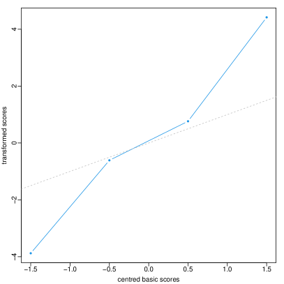
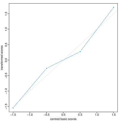
Figure 1: Oesophageal cancer data: new scores versus equally spaced scores using the $S_{U}$ (left panel) and $g$-and-$h$ distribution (right panel); the grey dashed line is the identity.

Given the essential coincidence of the numerical outcomes reported in Tables 1 and 2, consideration about the relative merits of the classical and the new methodology rests on the more qualitative side, especially interpretability of the outcome. In this respect, it seems advantageous to be provided with a set of scores which quantify in a simple way how the four categories of alcgp are actually spaced. For further simplification, especially for convenience of non-specialist readers, one could linearly transform the scores to more easily readable ones. For instance, we could transform the scores so that the first two of them are $(1,2)$, which leads to the values $(1,2,2.42,3.54)$ for both the $S_{U}$ and the $g$-and-$h$ variant.

We have not yet mentioned a method for constructing scores which has a long tradition in statistical practice, namely the use of mid-values of the alcgp classes. This method is has the advantage of simplicity, but it runs into difficulty when the class in unbounded. In the example under consideration, the upper class of alcgp is $[120,\infty)$ and the selection of a sensible ‘mid-value’ introduces another element of subjective choice. In fact, it is quite common that at least one of the extremal classes of an order factored constructed by grouping of continuous values is unbounded. Another limitation of this option is that it is feasible only for factors obtained by grouping of an underlying continuous variable; it is not feasible with a different genesis of the factor, such as in the case considered in the next numerical illustration.

3.2 Diamond pricing data

Various packages within the R environment, such as ggplot2, include the dataset diamonds which comprises 10 characteristics of 54,940 round cut diamonds. The main determinants of the price are four classical variables of interest, often collectively denoted as “the 4C’s”, which are as follows:

carat	denotes weight (1 carat equals $0.2$ grams);
clarity	indicates how clear the diamond is,
	with levels I1 (worst), SI2, SI1, VS2, VS1, VVS2, VVS1, IF (best);
color	the diamond colour, from D (best) to J (worst);
cut	indicates the quality of the cut, with levels Fair, Good, Very Good, Premium, Ideal.

Among these, only carat is of numeric type; all the others are of ordinal type. The purpose of the exercise is to find a simple rule for predicting the monetary value (in USD) from the 4C’s variables. Given the large number of cases in the dataset and the purely illustrative aim of the present demonstration, we examined a small subset of the data, namely those with row number $1,101,201,\ldots$.

The instinctive starting point is a linear model with response variable price and explanatory variables carat, clarity, color and cut. However, graphical exploration of the data exhibited noticeable curvature of the response variable as well as increasing dispersion as carat increases. Use of the Box-Cox transformation indicated $0.436$ as the appropriate power transformation for linearizing the relationship, although this does not quite stabilizes the residual dispersion. For simplicity, the power value $0.436$ has been approximated to $0.5$ even if this value is slightly outside the pertaining confidence interval, hence using sqrt(price) as the response variable. The ordered factors have been initially included using orthogonal polynomials at the maximal degree allowed by their number of levels, which are $8,7,5$, respectively. Observations numbered $(518,519,523)$ resulted to be clear outliers with high leverage; after their removal, there were $537$ observations left. In addition, several higher order components of the polynomials could be removed, leading to the model summarized in Table 3.

Table 3: Diamond pricing data: summary ingredients of the linear model for response variable sqrt(price) using orthogonal polynomials for expressing the ordered factors effects.

	Estimate	Std. Error	z value	Pr($>$$|$z$|$)
(Intercept)	1.194	0.75	1.60	0.11
carat	65.317	0.71	92.31	0.00
clarity.L	24.154	1.58	15.25	0.00
clarity.Q	-11.701	1.24	-9.42	0.00
clarity.C	3.610	1.24	2.90	0.00
color.L	-13.271	0.96	-13.76	0.00
color.Q	-1.907	0.89	-2.13	0.03
color.C	1.979	0.85	2.33	0.02
color^4	3.369	0.78	4.30	0.00
cut.L	1.882	0.85	2.21	0.03
Residual std. deviation: 6.74 on 527 degrees of freedom

For this numerical illustration, we apply the proposed method to two factors simultaneously, namely clarity and color, making use of the $g$-and-$h$ and the $\mathrm{sinh}$–$\mathrm{arcsinh}$ distribution. Since both distributions feature two parameters, the numerical optimization for minimizing the residual variance involves a four-dimensional search in both cases. Similarly to the illustration of Section 3.1, the target criterion for choosing the trasformation parameters agrees with the criterion for fitting the original model, that is, the residual variance in case of a linear model; again, penalized variants of the residual variance are possible. The outcome of the fitting process is summarized in Table 4. We do not report the analogous values using the $S_{U}$ distribution, but they were qualitatively similar to those for the other two distributions.

Table 4: Diamond pricing data: summary ingredients of the linear model for response variable sqrt(price) when the factors clarity and color are expressed via constructed sets of scores. The first sub-table employs the $g$-and-$h$ distribution; the second sub-table refers to the $\mathrm{sinh}$–$\mathrm{arcsinh}$ distribution.

g-and-h distribution Estimate Std. Error t value Pr($>$$|$t$|$) (Intercept) 6.448 0.67 9.68 0.00 carat 65.001 0.71 91.03 0.00 clarity.score 8.618 0.47 18.52 0.00 color.score -6.811 0.49 -13.98 0.00 cut.L 2.003 0.87 2.31 0.02 Residual std.  deviation: 6.90 on 532 degrees of freedom

$\mathrm{sinh}$–$\mathrm{arcsinh}$ distribution Estimate Std. Error t value Pr($>$$|$t$|$) (Intercept) 23.105 1.00 23.05 0.00 carat 65.087 0.71 91.72 0.00 clarity.score 0.000 0.00 18.72 0.00 color.score -0.072 0.01 -14.26 0.00 cut.L 2.028 0.86 2.35 0.02 Residual std. deviation: 6.85 on 532 degrees of freedom

Taking the residual standard deviation as the reference ingredient in Table 4, we see a modest increase with respect to the value, $6.74$, of Table 3. On the other hand, there is a substantial simplification of the model complexity, which may more than compensate the limited increase of residual standard deviation. A formal comparison between the model of Table 3 and those of Table 4 is not feasible by standard procedures, because the models are non-nested, and in addition because of the qualitative difficulty of making allowance for the parameters of the transformation distributions; on a broadly connected point, see also the discussion of Section 4.

A specific note is due for the sub-table of the $\mathrm{sinh}$-$\mathrm{arcsinh}$ distribution. The very small absolute values of some estimates reflect the very large size of the constructed scores, especially so for clarity whose scores range up to $10^{9}$. Correspondingly, the clarity.score estimate appearing as $0.000$ in Table 4 becomes $7.83{\times}10^{-9}$ with standard error $4.18{\times}10^{-10}$ when written in scientific notation. In practical work, these scores could simply be scaled down to more manageable values, with matching increase of the estimates and standard errors. However, for the present illustration, we have preferred to report the outcome in its original form.

4 Some miscellaneous remarks

As stated in the introductory section, the aim of this proposal is to retain an adequate fitting, as compared to the currently standard technique based on the polynomial representation of the factor, while providing a plainer interpretation of the resulting model. Note that the methodology does not attempt to improve on the polynomial-based fitting when one is ready to set a sufficiently high degree of the polynomial, since this scheme will eventually involve as many parameters as the number of factor levels. On the other hand, a high-degree polynomial model goes against the idea of a parsimonious model, and it is not desirable from an interpretational viewpoint, while these aspects constitute key motivations for the present proposal.

Clearly, the proposed method can be employed in a variety of situations, not only linear or generalized linear models. The method is suitable for any formulation where the response variable is regulated, possibly through some transformation, by some predictor which incorporates the ordered factors. For instance, proportional hazard models for the analysis of survival data represent another possibility. In this case, the natural criterion for choosing the transformation parameter is maximization of the partial log-likelihood, possibly in some penalized form.

In the numerical cases which have been examined, including those which have not been reported here, adequate linearization of the factor effect could always be achieved with some suitably chosen parameters of the transformation. It could possibly happen that in harder problems such a linearization may be not attainable; in these cases, one could consider introducing a parametric family of distributions with increased flexibility, involving more than two shape parameters. For instance, one could consider the generalized hyperbolic distribution, which allows higher flexibility, although at the cost of an higher computational effort and often increased difficulties at the fitting stage.

A possible remark concerning the interpretation of the outcome summarized in Table 2 and 4 is that the <factor>.score coefficients vary with the parameters of the transformation distribution and we should consider whether this variability should be taken into account. More explicitly, the question is whether the evaluation of the variance of the parameter of interest, namely the coefficients of alcp.score, clarity.score and color.score, should include its inflation due to the estimation step of the transformation parameters. This sort of consideration is similar to one raised for the Box-Cox transformation in other situations. Recall that, while the Box-Cox transformation had been introduced for the response variabile, it has been used also for transforming explanatory variables. The issue is quite broad and beyond the scope of the present note, but we mention at least the situation examined by Siqueira & Taylor, (1999) because of the similarity with the one of Section 3.1, since they also deal with a logistic model, the difference being that they consider a Box-Cox transformation of a continuous explanatory variable. One simple way of addressing the issue of variance inflation here is similar to the one denoted ‘conditional’ by Siqueira & Taylor, (1999), but its essence can be linked to the argumentation of Box & Cox, (1982). Under this view, the interpretation of the regression coefficient must refer to a fixed transformation, hence to fixed transformation parameters, since the assessment across different transformations would imply combining values on different and incomparable scales, preventing any sound scientific interpretation.

The proposed methodology has been implemented in an R package freely available at https://CRAN.R-project.org/package=smof whose documentation also shows how to reproduce the numerical illustrations of Section 3.

Acknowledgements

I am grateful to Sandy Weisberg and Alan Agresti for a number of insightful remarks on a preliminary sketch of this proposal, leading to a substantially improved presentation. Additional constructive comments have been provided by an associate editor and four reviewers of the submitted paper, to whom I also express my gratitude for stimulating an improved exposition.

References

- Agresti, (2010) Agresti, A. (2010). Analysis of Ordinal Categorical Data. J. Wiley & Sons, second edition.
- Armitage, (1955) Armitage, P. (1955). Tests for linear trends in proportions and frequencies. Biometrics, 11, 375–386.
- Box & Cox, (1982) Box, G. E. P. & Cox, D. R. (1982). An analysis of transformations revisited, rebutted. J. Amer. Statist. Assoc., 77(209–210).
- Breslow & Day, (1980) Breslow, N. E. & Day, N. E. (1980). Statistical Methods in Cancer Research, volume 1 – The analysis of case-control studies. International Agency for Research Cancer, World Health Organization.
- Chambers & Hastie, (1993) Chambers, J. M. & Hastie, T. J. (1993). Statistical models. In Statistical Models in S chapter 2. Wadsworth & Brooks/Cole.
- Gertheiss & Tutz, (2009) Gertheiss, J. & Tutz, G. (2009). Penalized regression with ordinal predictors. Int. Statist. Rev., 77, 345–365.
- Graubard & Korn, (1987) Graubard, B. I. & Korn, E. L. (1987). Choice of column scores for testing independence in ordered contingency tables. Biometrics, 43, 471–476.
- Hoaglin, (1984) Hoaglin, D. C. (1984). Summarizing shape numerically: the -and- distributions. In D. C. Hoaglin, F. Mosteller, & J. W. Tukey (Eds.), Exploring Data Tables, Trends, and Shapes chapter 11. J. Wiley & Sons.
- Johnson, (1949) Johnson, N. L. (1949). Systems of frequency curves generated by methods of translation. Biometrika, 36, 146–176.
- Johnson et al., (1994) Johnson, N. L., Kotz, S., & Balakrishnan, N. (1994). Continuous Univariate Distributions, volume 1. J. Wiley & Sons, second edition.
- Jones & Pewsey, (2009) Jones, M. C. & Pewsey, A. (2009). Sinh-arcsinh distributions. Biometrika, 96, 761–780.
- Pasta, (2009) Pasta, D. J. (2009). Learning when to be discrete: continuous vs. categorical predictors. In SAS Global Forum 2009 (pp. Paper 248–2009).
- R Core Team, (2022) R Core Team (2022). R: A Language and Environment for Statistical Computing. R Foundation for Statistical Computing, Vienna, Austria.
- Siqueira & Taylor, (1999) Siqueira, A. L. & Taylor, J. M. G. (1999). Treatment effects in a logistic model involving the Box-Cox transformation. J. Amer. Statist. Assoc., 94, 240–246.
- Solomon & Stephens, (1978) Solomon, H. & Stephens, M. A. (1978). Approximations to density functions using Pearson curves. J. Amer. Statist. Assoc., 73, 153–160.
- Tutz & Gertheiss, (2016) Tutz, G. & Gertheiss, J. (2016). Regularized regression for categorical data. Stat. Modelling, 16, 161–200.
- Williams, (2020) Williams, R. A. (2020). Ordinal independent variables. In P. Atkinson, S. Delamont, A. Cernat, J. W. Sakshaug, & R. A.Williams (Eds.), Linear Regression. SAGE Research Methods Foundations.
- Winer, (1962) Winer, B. J. (1962). Statistical Principles in Experimental Design. McGraw-Hill.
- Winship & Mare, (1984) Winship, C. & Mare, R. D. (1984). Regression models with ordinal variables. American Sociological Review, 49, 512–525.