Improving LaCAM for Scalable Eventually Optimal Multi-Agent Pathfinding

Abstract

This study extends the recently-developed LaCAM algorithm for multi-agent pathfinding (MAPF). LaCAM is a sub-optimal search-based algorithm that uses lazy successor generation to dramatically reduce the planning effort. We present two enhancements. First, we propose its anytime version, called $\text{LaCAM}^{\ast}$, which eventually converges to optima, provided that solution costs are accumulated transition costs. Second, we improve the successor generation to quickly obtain initial solutions. Exhaustive experiments demonstrate their utility. For instance, $\text{LaCAM}^{\ast}$ sub-optimally solved 99% of the instances retrieved from the MAPF benchmark, where the number of agents varied up to a thousand, within ten seconds on a standard desktop PC, while ensuring eventual convergence to optima; developing a new horizon of MAPF algorithms.

1 Introduction

The multi-agent pathfinding (MAPF) problem aims to assign collision-free paths for multiple agents on a graph. To date, various MAPF algorithms have been developed, motivated by various applications such as warehouse automation Wurman et al. (2008). Ideal MAPF algorithms will be complete, optimal, quick, and scalable. However, there is generally a tradeoff between the former two and the latter two. Conversely, the primary challenge of developments in MAPF algorithms is to guarantee solvability and solution quality, while suppressing planning efforts to secure speed and scalability.

To break this tradeoff, we present two enhancements to the recently-developed algorithm called LaCAM (lazy constraints addition search for MAPF) Okumura (2023). It is complete, sub-optimal, and search-based (akin to $\text{A}^{\ast}$ search) that uses lazy successor generation. The first enhancement is its anytime version called $\text{LaCAM}^{\ast}$ that eventually converges to optima, provided that solution costs are accumulated transition costs. Since solving MAPF optimally is computationally intractable Yu and LaValle (2013), one practical approach to large instances is obtaining sub-optimal solutions and then refining their quality as time allows. $\text{LaCAM}^{\ast}$ meets such demands. The second enhancement is for the successor generation, i.e., tuning of the PIBT algorithm Okumura et al. (2022), so as to quickly obtain initial solutions.

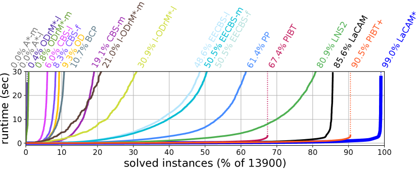
	algorithm	reference	solvability	optimality	metrics
$\blacksquare$	$\text{A}^{\ast}$	Hart et al. (1968)	complete	optimal	m, l
$\blacksquare$	OD	Standley (2010)	complete	sub-optimal	(greedy)
$\blacksquare$$\blacksquare$	ODrM∗	Wagner and Choset (2015)	complete	optimal	m, l
$\blacksquare$$\blacksquare$	I-ODrM∗	Wagner and Choset (2015)	complete	bnd. sub-opt.	m, l
$\blacksquare$	BCP	Lam et al. (2022)	solution cmp.	optimal	f
$\blacksquare$$\blacksquare$$\blacksquare$	CBS	Sharon et al. (2015)	solution cmp.	optimal	f, m, l
$\blacksquare$$\blacksquare$$\blacksquare$	EECBS	Li et al. (2021c)	solution cmp.	bnd. sub-opt.	f, m, l
$\blacksquare$	PP	Silver (2005)	incomplete	sub-optimal
$\blacksquare$	LNS2	Li et al. (2022)	incomplete	sub-optimal
$\blacksquare$$\blacksquare$	PIBT(+)	Okumura et al. (2022)	incomplete	sub-optimal
$\blacksquare$	LaCAM	Okumura (2023)	complete	sub-optimal
$\blacksquare$	$\text{LaCAM}^{\ast}$	this paper	complete	eventually opt.	m, l

Figure 1: Performance on the MAPF benchmark. upper: The number of solved instances among 13,900 instances on 33 four-connected grid maps, retrieved from Stern et al. (2019). The size of agents varies up to 1,000. ‘-f,’ ‘-m,’ and ‘-l’ respectively mean that an algorithm tries to minimize flowtime, makespan, or sum-of-loss. The scores of $\text{LaCAM}^{\ast}$ are for initial solutions. lower: Representative or state-of-the-art MAPF algorithms. “solution cmp.” means that an algorithm ensures to find solutions for solvable instances but it never identifies unsolvable ones. “bnd. sub-opt.” means a bounded sub-optimal algorithm. Their sub-optimality was set to five.

With these enhancements, we empirically demonstrate that $\text{LaCAM}^{\ast}$ can break the trade-off. For instance, it sub-optimally solved 99% of the instances retrieved from the MAPF benchmark Stern et al. (2019) within ten seconds while guaranteeing the eventual optimality, on a standard desktop PC. As illustrated in Fig. 1, this result is beyond frontiers of existing MAPF algorithms. In what follows, we present preliminaries, $\text{LaCAM}^{\ast}$, improved successor generation, empirical results, and discussion in order. The appendix and code are available at https://kei18.github.io/lacam2/.

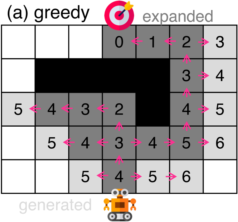
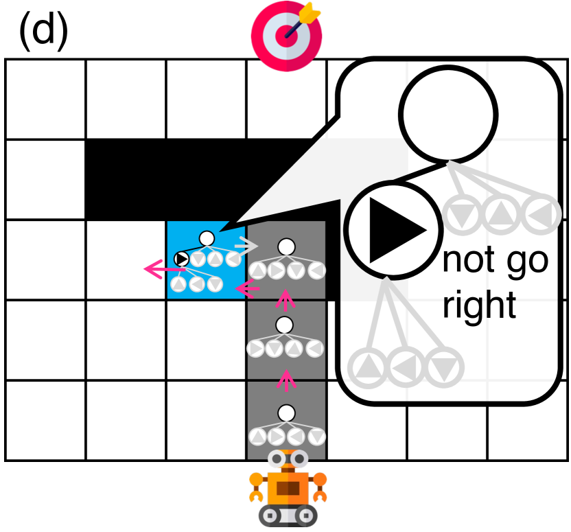
Figure 2: Illustration of LaCAM using single-agent grid pathfinding.

2 Preliminaries

2.1 Notation, Problem Definition, and Assumption

Notations.

$S[k]$ denotes the $k$-th element of the sequence $S$, where the index starts at one. For convenience, we use $\bot$ as an “undefined” or “not found” sign.

Instance.

An MAPF instance is defined by a graph $G=(V,E)$, a set of agents $A=\{1,\ldots,n\}$, a tuple of distinct starts $\mathcal{S}=(s_{i}\in V)^{i\in A}$ and goals $\mathcal{G}=(g_{i}\in V)^{i\in A}$.

Configuration.

A configuration is a tuple of locations for all agents. For instance, $\mathcal{Q}=(v_{1},v_{2},\ldots,v_{n})\in V^{|A|}$ is a configuration, where $\mathcal{Q}[i]=v_{i}$ is the location of agent $i\in A$. The start and goal configurations are $\mathcal{S}$ and $\mathcal{G}$, respectively.

Collision and Connectivity.

A configuration $\mathcal{Q}$ has a vertex collision when there is a pair of agents $i,j\in A,i\neq j$, such that $\mathcal{Q}[i]=\mathcal{Q}[j]$. Two configurations $X$ and $Y$ have an edge collision when there is a pair of agents $i,j\in A,i\neq j$, such that $X[i]=Y[j]\land Y[i]=X[j]$. Let $\mathsf{neigh}(v)$ be a set of vertices adjacent to $v\in V$. Two configurations $X$ and $Y$ are connected when $Y[i]\in\mathsf{neigh}(X[i])\cup\{X[i]\}$ for all $i\in A$, and, there are neither vertex nor edge collisions in $X$ and $Y$.

Decision Problem.

Given an MAPF instance, an MAPF problem is a decision problem that asks existence of a sequence of configurations $\Pi=(\mathcal{Q}_{0},\mathcal{Q}_{1},\ldots,\mathcal{Q}_{k})$, such that $\mathcal{Q}_{0}=\mathcal{S}$, $\mathcal{Q}_{k}=\mathcal{G}$, and any two consecutive configurations in $\Pi$ are connected. A solution to MAPF is a $\Pi$ that satisfies the conditions. To align with the literature, the index of $\Pi$ exceptionally starts at zero (i.e., $\Pi[0]=\mathcal{Q}_{0}$). An algorithm is said to be complete when it returns solutions for solvable instances and reports non-existence for unsolvable instances. Otherwise, it is called incomplete.

Optimization Problems.

Given a transition (or edge) cost between two configurations, $\mathsf{cost}_{e}:V^{|A|}\times V^{|A|}\mapsto\mathbb{R}_{\geq 0}$, we aim at minimizing accumulated transition costs of a solution $\Pi$, denoted as $\mathsf{cost}(\Pi)\mathrel{\mathop{:}}=\sum_{t=0}^{k-1}\mathsf{cost}_{e}\bigl{(}\Pi[t],\Pi[t+1]\bigr{)}$. This notation can represent various optimization metrics. For instance, $\mathsf{cost}$ is called makespan when $\mathsf{cost}_{e}(X,Y)\mathrel{\mathop{:}}=1$. It is called sum-of-fuels (aka. total travel distance) when $\mathsf{cost}(X,Y)\mathrel{\mathop{:}}=|\{i\in A;X[i]\neq Y[i]\}|$. Sum-of-loss counts actions of non-staying at goals, defined by $\mathsf{cost}_{e}(X,Y)\mathrel{\mathop{:}}=|\{i\in A\mid\lnot(X[i]=Y[i]=g_{i})\}|$. A solution $\Pi$ is optimal when there is no solution $\Pi^{\prime}$ such that $\mathsf{cost}(\Pi^{\prime})<\mathsf{cost}(\Pi)$.

Remarks for Flowtime.

Another common metric of MAPF is flowtime (aka. sum-of-costs): $\sum_{i\in A}t_{i}$, where $t_{i}\leq k$ is the earliest timestep such that $\Pi[t_{i}][i]=\Pi[t_{i}+1][i]=\ldots=\Pi[k][i]=g_{i}$. The difference from sum-of-loss is cost contribution of agents who once reach their goal and leave there temporarily. The flowtime is history-dependent on paths of each agent; hence, it is impossible to represent as it is with accumulative costs. Instead, this paper considers sum-of-loss as seen in Standley (2010); Wagner and Choset (2015).

Admissible Heuristic.

We assume an admissible heuristic $\mathsf{h}:V^{|A|}\mapsto\mathbb{R}_{\geq 0}$, such that $\mathsf{h}(Q)$ is always the optimal cost from $\mathcal{Q}$ to $\mathcal{G}$ or less; e.g., $\mathsf{h}(\mathcal{Q})\mathrel{\mathop{:}}=\sum_{i\in A}\mathsf{dist}(\mathcal{Q}[i],g_{i})$ is available for the sum-of-{loss, fuels}, where $\mathsf{dist}:V\times V\mapsto\mathbb{N}_{\geq 0}$ is the shortest path length on $G$.

Understanding MAPF as Graph Pathfinding.

Using configurations, consider a graph $H$ comprising vertices that represent configurations, and edges that represent the connectivity of configurations. Then, by regarding $\mathcal{S}$ and $\mathcal{G}$ as start and goal vertices respectively, optimal MAPF is equivalent to the shortest pathfinding problem on $H$. This is a key perspective to understand LaCAM^(∗).

2.2 LaCAM

LaCAM Okumura (2023) was originally developed as a sub-optimal complete MAPF algorithm. In a nutshell, it is a graph pathfinding algorithm, like $\text{A}^{\ast}$, but some parts are specific to MAPF. Below, we provide the essence of the graph pathfinding part, using an example of single-agent grid pathfinding. The details of the MAPF-specific part are delivered in the appendix.

Classical Search.

See Fig. 2a that illustrates how a typical search scheme solves grid pathfinding. Specifically, we show the greedy best-first search with a heuristic of the Manhattan distance. Here, a location of the agent corresponds to a configuration (aka. state) of the search. From the start configuration, the search generates three successor nodes: left, up, and right. Each node corresponds to one configuration. The search then takes one of the generated nodes according to the heuristic, and generates successors. This procedure continues until finding the goal configuration.

Branching Factor.

Consider how many nodes are generated to estimate the search effort. Though the solution length is 8, 22 nodes are generated. This number is related to the number of connected configurations (i.e., branching factor). It is four in grid pathfinding, therefore, the number of node generations remains acceptable. However, the branching factor of MAPF is exponential for the number of agents. Consequently, the generation itself becomes intractable. This is why a vanilla $\text{A}^{\ast}$ is hopeless to solve large MAPF instances.

Configuration Generator.

LaCAM tries to relieve this huge-branching-factor issue when a configuration generator is available. Given a configuration and constraints, it generates a connected configuration following constraints. Constraints should be embodied by each domain. In this example, consider a constraint as a prohibition of direction, such as not moving up, left, right, or down.

Constraint Tree.

Each search node of LaCAM contains not only a configuration but also constraints, taking the form of a tree structure. For each node invoke, LaCAM gradually develops the tree by low-level search, implemented by, e.g., breadth-first search (BFS). A node on the tree has a constraint and represents several constraints by tracing a path to the root.

Search Flow.

We now explain LaCAM using Fig. 2b–e, with a depth-first search (DFS) style. The attempt to find a sequence of configurations is called high-level search. At first, a search node of the start is examined (Fig. 2b). The node poses no constraints for the first invoke, meaning that the configuration generator can output any connected configuration. Suppose that the generator outputs an “up” configuration, following the Manhattan distance guide, illustrated by the pink arrow. Preparing for the second invoke, the node expands a constraint tree with new constraints (e.g., “not go up”). The high-level search does not discard the examined node immediately, rather, it discards when all connected configurations have been generated (i.e., when the low-level search completes). Next, Fig. 2c–d show an example of the second invoke of nodes. In Fig. 2c, the generator outputs an already-known configuration. Since this example assumes DFS, LaCAM examines the blue-colored node again in Fig. 2d. This time, the generator must follow a constraint “not go right” and its parent “no constraint.” The example then generates a “left” configuration. The search continues until finding the goal (Fig. 2e) and obtains a solution path by backtracking.

Adaptation to MAPF.

With appropriate designs of constraints and tree construction, LaCAM can be an exhaustive search and guarantees completeness for graph pathfinding problems. In Okumura (2023), such an example is shown for MAPF by letting a constraint specify which agent is where in the next configuration. Moreover, LaCAM can greatly decrease the number of node generations if the configuration generator is promising in outputting configurations that are close to the goal. This reduction could be a silver bullet to achieve quick planning, especially in planning problems where the branching factor is huge like MAPF. The remaining question is a realization of good configuration generators. In the original paper, PIBT (priority inheritance with backtracking) Okumura et al. (2022) served as it, explained in Sec. 2.3.

Pseudocode.

Algorithm 1 shows DFS-based LaCAM. Each search node $\mathcal{N}$ stores (i) a configuration, (ii) a constraint tree embodied by a queue (assuming BFS) and (iii) a pointer to a parent node (see 4). Nodes are stored in an $\mathit{Open}$ list and $\mathit{Explored}$ table, akin to general search schema, and are processed one by one. We abstract how to create constraint trees for MAPF by 11, which is elaborated in the appendix.

Algorithm 1 LaCAM. $\mathcal{C}_{\text{init}}$ means “no constraint.”

1:

2:

3: initialize $\mathit{Open}$, $\mathit{Explored}$ $\triangleright$ stack, hash table

4: $\mathcal{N}^{\text{init}}\leftarrow\bigl{\langle}~{}\mathit{config}:\mathcal{S},\mathit{tree}:\llbracket~{}\mathcal{C}^{\text{init}}~{}\rrbracket,\mathit{parent}:\bot~{}\bigr{\rangle}$

5: $\mathit{Open}.\mathsf{push}\left(\mathcal{N}^{\text{init}}\right)$;  $\mathit{Explored}[\mathcal{S}]=\mathcal{N}^{\text{init}}$

6: while $\mathit{Open}\neq\emptyset$ do

7:    $\mathcal{N}\leftarrow\mathit{Open}.\mathsf{top}()$

8:    if $\mathcal{N}.\mathit{config}=\mathcal{G}$ then return $\mathsf{backtrack}(\mathcal{N})$

9:    if $\mathcal{N}.\mathit{tree}=\emptyset$ then $\mathit{Open}.\mathsf{pop}()$; continue $\triangleright$ discard node

10:    $\mathcal{C}\leftarrow\mathcal{N}.\mathit{tree}.\mathsf{pop}()$ $\triangleright$ get constraint

11:    $\mathsf{low\_level\_expansion}(\mathcal{N},\mathcal{C})$ $\triangleright$ proceed low-level search

12:    $\mathcal{Q}^{\text{new}}\leftarrow\mathsf{configuration\_generator}(\mathcal{N},\mathcal{C})$

13:    if $\mathcal{Q}^{\text{new}}=\bot$ then continue $\triangleright$ generator may fail

14:    if $\mathit{Explored}\left[\mathcal{Q}^{\text{new}}\right]\neq\bot$ then continue

15:    $\mathcal{N}^{\text{new}}\leftarrow\langle~{}\mathit{config}:\mathcal{Q}^{\text{new}},\mathit{tree}:\left\llbracket~{}\mathcal{C}^{\text{init}}~{}\right\rrbracket,\mathit{parent}:\mathcal{N}~{}\bigr{\rangle}$

16:    $\mathit{Open}.\mathsf{push}\left(\mathcal{N}^{\text{new}}\right)$; $\mathit{Explored}\left[\mathcal{Q}^{\text{new}}\right]=\mathcal{N}^{\text{new}}$

17: return NO_SOLUTION

Algorithm 2 PIBT

1:

2:

3: for $i\in A$ do;  if $\mathcal{Q}^{\text{to}}[i]=\bot$ then $\mathsf{PIBT}(i)$

4: return $\mathcal{Q}^{\text{to}}$

5: procedure $\mathsf{PIBT}$($i$) $\triangleright$ return VALID or INVALID

6:    $C\leftarrow\mathsf{neigh}\left(\mathcal{Q}^{\text{from}}[i]\right)\cup\left\{\mathcal{Q}^{\text{from}}[i]\right\}$ $\triangleright$ candidate vertices

7:    sort $C$ in ascending order of $\mathsf{dist}(u,g_{i})$ where $u\in C$

8:    for $v\in C$ do

9:       if collisions in $\mathcal{Q}^{\text{to}}$ supposing $\mathcal{Q}^{\text{to}}[i]=v$ then continue

10:       $\mathcal{Q}^{\text{to}}[i]\leftarrow v$

11:       if $\exists j\in A~{}\text{s.t.}~{}j\neq i\land\mathcal{Q}^{\text{from}}[j]=v\land\mathcal{Q}^{\text{to}}[j]=\bot$ then

12:          if $\mathsf{PIBT}(j)=\texttt{INVALID}$ then continue       

13:       return VALID $\triangleright$ assignment done    

14:    $\mathcal{Q}^{\text{to}}[i]\leftarrow\mathcal{Q}^{\text{from}}[i]$; return INVALID

Figure 3: Concept of PIBT. $\mathcal{Q}^{\text{from}}$ is illustrated. Bold arrows represent assignments of $\mathcal{Q}^{\text{to}}$. (a) Consider a fixed assignment order of $i$, $k$, and $j$. If $i$ and $k$ are assigned following the illustrated arrows, $j$ has no candidate vertex as $\mathcal{Q}^{\text{to}}[j]$ (annotated with $\times$). (b)  This pitfall is overcome by doing the assignment for $j$ prior to $k$, reacting to $i$’s assignment request.

2.3 PIBT

PIBT Okumura et al. (2022) was originally developed to solve MAPF iteratively. In a nutshell, it is a configuration generator, which generates a new connected configuration ($\mathcal{Q}^{\text{to}}$), given another ($\mathcal{Q}^{\text{from}}$) as input. By continuously generating configurations, PIBT can generate a solution for MAPF.

Concept.

To determine $\mathcal{Q}^{\text{to}}$, PIBT sequentially assigns a vertex to each agent while avoiding assignments that trigger collisions. This assignment order adaptively changes. Specifically, before fixing $\mathcal{Q}^{\text{to}}[i]$ to $v\in\mathsf{neigh}(\mathcal{Q}^{\text{from}}[i])\cup\{\mathcal{Q}^{\text{from}}[i]\}$, PIBT first checks the existence of $j\in A$ such that $\mathcal{Q}^{\text{from}}[j]=v$. If such $j$ exists, $j$ may have no candidate vertex for $\mathcal{Q}^{\text{to}}[j]$, due to collision avoidance (see Fig. 3a). Therefore, PIBT next determines $\mathcal{Q}^{\text{to}}[j]$ prior to locations of other agents (e.g., $k$ in Fig. 3). This scheme is called priority inheritance. If $\mathcal{Q}^{\text{to}}[j]$ is successfully assigned, $\mathcal{Q}^{\text{to}}[i]$ is fixed to $v$ (Fig. 3b); otherwise, $\mathcal{Q}^{\text{to}}[i]$ needs to take another vertex other than $v$.

Pseudocode.

Algorithm 2 implements the concept above, by recursively calling a procedure $\mathsf{PIBT}$ (5–), which takes an agent $i$ and eventually assigns $\mathcal{Q}^{\text{to}}[i]$. The assignment attempts of Lines 8–13 are performed for candidate vertices regarding $\mathcal{Q}^{\text{from}}[i]$, in ascending order of the distance toward $g_{i}$. The attempts continue until $\mathcal{Q}^{\text{to}}[i]$ is determined, resulting in VALID outcome (13). When all attempts failed, $\mathsf{PIBT}(i)$ assigns $\mathcal{Q}^{\text{from}}[i]$ to $\mathcal{Q}^{\text{to}}[i]$ and returns INVALID (14). Priority inheritance is triggered as necessary, taking the form of calling $\mathsf{PIBT}$ for another agent $j$ (12). The success of priority inheritance triggers receipt of VALID; otherwise, INVALID is backed, and then $i$ continues the assignment attempts.

Dynamic Priorities.

In addition to priority inheritance, PIBT prioritizes assignments for agents that are not on their goal, which is done by sorting $A$ of 3 in that way. This scheme is convenient for lifelong scenarios wherein all agents are not necessarily being goals simultaneously.

3 $\text{LaCAM}^{\ast}$: Eventually Optimal Algorithm

Algorithm 3 presents $\text{LaCAM}^{\ast}$. The same lines as LaCAM (Alg. 1) are grayed out. The blue-colored lines are not necessary from the theoretical side but are effective in speeding up the search. The main differences from LaCAM are two: (i) it continues the search when finding the goal configuration $\mathcal{G}$, and, (ii) it rewrites parent relations between search nodes as necessary. For convenience, the transition cost $\mathsf{cost}_{e}$ and admissible heuristic $\mathsf{h}$ can take nodes as arguments, instead of configurations. Below, the updated parts are explained.

Keeping Goal Node.

$\text{LaCAM}^{\ast}$ retains the goal node $\mathcal{N}^{\text{goal}}$, rather than immediately returning solutions when first finding the goal $\mathcal{G}$ (9). The search terminates when there is no remaining node in $\mathit{Open}$; otherwise, there is an interruption from users such as timeout (7). A solution is then constructed by backtracking from $\mathcal{N}^{\text{goal}}$ (Lines 31–32). Doing so makes $\text{LaCAM}^{\ast}$ an anytime algorithm, that is, after finding the goal node, it is interruptible whenever a solution is required, while gradually refining solution quality as time allows.

Search Node Ingredients.

Each high-level node contains a set $\mathit{neigh}$ that stores connected configurations (i.e., nodes) and g-value that represents cost-to-come from the start $\mathcal{S}$ (5). They are initialized and updated appropriately when finding a new configuration (Lines 27–30).

Updating Parents and Costs.

To maintain the optimality, when finding an already known configuration, $\text{LaCAM}^{\ast}$ updates $\mathit{neigh}$ (17). This is followed by updates of g-value and $\mathit{parent}$, performed by Dijkstra’s algorithm (Lines 19–24). Figure 4 illustrates the update.

Discarding Redundant Nodes.

Once the goal node is found, $\text{LaCAM}^{\ast}$ discards nodes that do not contribute to improving solution quality (10). It also revives nodes as necessary when their $g$-values are updated (26).

Theorem 1.

$\text{LaCAM}^{\ast}$ (Alg. 3) is complete and optimal.

Proof.

Consider Alg. 3 without blue lines (10 and 26); they just speed up the search without breaking the optimal search structure. In this proof, the term “path” refers to a sequence of connected configurations.

Algorithm 3 $\text{LaCAM}^{\ast}$. $\mathcal{C}_{\text{init}}$ means “no constraint.”

1:

2:

3:

4: initialize $\mathit{Open},\mathit{Explored}$; $\mathcal{N}^{\text{goal}}\leftarrow\bot$

5: ${\color[rgb]{0.6,0.6,0.6}\mathcal{N}^{\text{init}}\leftarrow\bigr{\langle}\mathit{config}:\mathcal{S},\mathit{tree}:\llbracket\mathcal{C}^{\text{init}}\rrbracket,\text{\it parent}:\bot,}~{}\mathit{neigh}:\emptyset,g:0{\color[rgb]{0.6,0.6,0.6}\bigr{\rangle}}$

6: $\mathit{Open}.\mathsf{push}\left(\mathcal{N}^{\text{init}}\right)$; $\mathit{Explored}[\mathcal{S}]=\mathcal{N}^{\text{init}}$

7: while ${\color[rgb]{0.6,0.6,0.6}\mathit{Open}\neq\emptyset}~{}\land~{}\lnot\mathsf{interrupt}()$ do

8:    $\mathcal{N}\leftarrow\mathit{Open}.\mathsf{top}()$

9:    if $\mathcal{N}.\mathit{config}=\mathcal{G}$ then $\mathcal{N}^{\text{goal}}\leftarrow\mathcal{N}$

10:    if $\spadesuit\land\mathsf{f}\left(\mathcal{N}^{\text{goal}}\right)\leq\mathsf{f}\left(\mathcal{N}\right)$ then $\mathit{Open}.\mathsf{pop}()$; continue

11:    if $\mathcal{N}.\mathit{tree}=\emptyset$ then $\mathit{Open}.\mathsf{pop}()$; continue

12:    $\mathcal{C}\leftarrow\mathcal{N}.\mathit{tree}.\mathsf{pop}()$

13:    $\mathsf{low\_level\_expansion}(\mathcal{N},\mathcal{C})$

14:    $\mathcal{Q}^{\text{new}}\leftarrow\mathsf{configuration\_generator}(\mathcal{N},\mathcal{C})$

15:    if $\mathcal{Q}^{\text{new}}=\bot$ then continue

16:    if $\mathit{Explored}\left[\mathcal{Q}^{\text{new}}\right]\neq\bot$ then

17:       $\mathcal{N}.\mathit{neigh}.\mathsf{append}\left(\mathit{Explored}\left[\mathcal{Q}^{\text{new}}\right]\right)$

18:       $\mathcal{D}\leftarrow\llbracket~{}\mathcal{N}~{}\rrbracket$ $\triangleright$ Dijkstra, priority queue of $g$-value

19:       while $\mathcal{D}\neq\emptyset$ do

20:          $\mathcal{N}^{\text{from}}\leftarrow\mathcal{D}.\mathsf{pop}()$

21:          for $\mathcal{N}^{\text{to}}\in\mathcal{N}^{\text{from}}.\mathit{neigh}$ do

22:            $g\leftarrow\mathcal{N}^{\text{from}}.g+\mathsf{cost}_{e}\left(\mathcal{N}^{\text{from}},\mathcal{N}^{\text{to}}\right)$

23:            if $g<\mathcal{N}^{\text{to}}.g$ then

24:               $\mathcal{N}^{\text{to}}.g\leftarrow g$; $\mathcal{N}^{\text{to}}.\mathit{parent}\leftarrow\mathcal{N}^{\text{from}}$; $\mathcal{D}.\mathsf{push}(\mathcal{N}^{\text{to}})$

25:               if $\spadesuit\land\mathsf{f}\left(\mathcal{N}^{\text{to}}\right)<\mathsf{f}\left(\mathcal{N}^{\text{goal}}\right)$ then $\mathit{Open}.\mathsf{push}\left(\mathcal{N}^{\text{to}}\right)$                             

26:    else

27:       ${\color[rgb]{0.6,0.6,0.6}\mathcal{N}^{\text{new}}\leftarrow}\begin{aligned} {\color[rgb]{0.6,0.6,0.6}\bigl{\langle}}&{\color[rgb]{0.6,0.6,0.6}\mathit{config}:\mathcal{Q}^{\text{new}},\mathit{tree}:\llbracket\mathcal{C}^{\text{init}}\rrbracket,\mathit{parent}:\mathcal{N},}\\ &\mathit{neigh}:\emptyset,g:\mathcal{N}.g+\mathsf{cost}_{e}\left(\mathcal{N},\mathcal{Q}^{\text{new}}\right){\color[rgb]{0.6,0.6,0.6}\bigr{\rangle}}\end{aligned}$

28:       $\mathit{Open}.\mathsf{push}\left(\mathcal{N}^{\text{new}}\right)$; $\mathit{Explored}\left[\mathcal{Q}^{\text{new}}\right]=\mathcal{N}^{\text{new}}$

29:       $\mathcal{N}.\mathit{neigh}.\mathsf{append}\left(\mathcal{N}^{\text{new}}\right)$    

30: if $\spadesuit\land\mathit{Open}=\emptyset$ then return $\mathsf{backtrack}\left(\mathcal{N}^{\text{goal}}\right)$ $\triangleright$ optimal

31: else if $\spadesuit$ then return $\mathsf{backtrack}\left(\mathcal{N}^{\text{goal}}\right)$ $\triangleright$ sub-optimal

32: else if $\mathit{Open}=\emptyset$ then return NO_SOLUTION

33: else return FAILURE

Figure 4: Updating parents and costs. Each circle is a search node (i.e., configuration), including its g-value of makespan. Arrows represent known neighboring relations. Among them, solid lines represent $\mathit{parent}$. The updated parts are red-colored. left: A new neighbor relationship, a red dashed arrow, has been found. right: Rewrite the search tree. Observe that the rewriting occurs in a limited part of the tree due to g-value pruning (23).

First, we introduce a directed graph $H$, where its vertex corresponds to a configuration. Initially, $H$ has only a start vertex $\mathcal{S}$. Then, the search iterations gradually develop $H$. When a new node is created (27), its configuration is added to $H$. An arc $(X,Y)$ of $H$ occurs when the search finds a connection from $X$ to $Y$, i.e., $\mathcal{N}^{Y}\in\mathcal{N}^{X}.\mathit{neigh}$.

We now prove that: ($\clubsuit$) for any configuration $\mathcal{Q}$ in $H$, a path from $\mathcal{S}$ to $\mathcal{Q}$ constructed by backtracking (i.e., by following $\mathcal{N}$.$\mathit{parent}$) is the shortest path in $H$, regarding accumulative transition costs, at the beginning of each search iteration. This is proven by induction. Initially, $H$ comprises only $\mathcal{S}$, satisfying $\clubsuit$. Assume now that $\clubsuit$ is satisfied in the previous iteration of Lines 7–29. In the next iteration, $H$ is updated by: (i) generating a new configuration (Lines 27–30), or (ii) finding a known configuration (Lines 17–24). Case (i) holds $\clubsuit$ because only a new vertex and an arc toward the vertex are added to $H$. Case (ii) holds $\clubsuit$ because only an arc is added for the node $\mathcal{N}$ (17), and then Lines 19–24 perform Dijkstra’s algorithm starting from $\mathcal{N}$ that maintains the tree structure of the shortest paths.

The search space of $\text{LaCAM}^{\ast}$ is finite (see Okumura (2023)); the search terminates in finite time. Each node eventually examines all connected configurations. Consequently, when terminated, $H$ includes all possible paths from $\mathcal{S}$ to $\mathcal{G}$ for solvable instances. Together with $\clubsuit$, $\text{LaCAM}^{\ast}$ returns an optimal solution, otherwise, reports the non-existence. ∎

Implementation Tips.

Following Okumura (2023), when finding an already known configuration at 16, our implementation reinserts the corresponding node to $\mathit{Open}$. Moreover, with a small probability (e.g., 0.1%), the implementation reinserts a node of $\mathcal{S}$ instead of the found one. Doing so enables the search to “escape” from configurations being bottlenecks. Such techniques relying on non-determinism have been seen in other search problems Kautz et al. (2002) and MAPF studies Cohen et al. (2018b); Andreychuk and Yakovlev (2018). Indeed, we informally observed that this random replacement slightly improved the success rate. Note that the optimality still holds with these modifications.

4 Improving Configuration Generator

The performance of LaCAM heavily relies on a configuration generator, therefore, the development of good generators is critical. The implementation in Okumura (2023) uses a vanilla PIBT of Alg. 2, resulting in poor performances in several scenarios, especially in instances with narrow corridors. This is because PIBT itself often fails such scenarios, hence being an ineffective guide for LaCAM. This section elaborates on this phenomenon and presents an improved version.

4.1 Failure Analysis of PIBT

As seen in Sec. 2.3, PIBT sequentially assigns the next locations for agents. Since this order prioritizes agents being not on their goals, livelock situations might be triggered. See Fig. 5; two agents reach their goal vertex periodically but PIBT never reaches the goal configuration.

LaCAM can break such livelocks by posing constraints. However, it may require significant effort because appropriate combinations of constraints should be explored. Even worse, with more agents, the search effort dramatically increases, as demonstrated in Table 1.

4.2 Enhancing PIBT by Swap

Livelocks in PIBT can be resolved by swap operation, originally developed in rule-based MAPF algorithms Luna and Bekris (2011); De Wilde et al. (2014). In short, this operation swaps locations of two agents using a vertex with a degree of three or more. Figure 6 shows an example. Here, we extract its essence and incorporate it into PIBT. Specifically, this is done by adjusting vertex scoring at 8 in Alg. 2.

Algorithm 4 procedure $\mathsf{PIBT}$ with swap

1: $C\leftarrow\mathsf{neigh}\left(\mathcal{Q}^{\text{from}}[i]\right)\cup\left\{\mathcal{Q}^{\text{from}}[i]\right\}$

2: sort $C$ in increasing order of $\mathsf{dist}(u,g_{i})$ where $u\in C$

3: $j\leftarrow\mathsf{swap\_required\_and\_possible}\left(i,C[1],\mathcal{Q}^{\text{from}}\right)$

4: if $j\neq\bot$ then reverse $C$

5: for $v\in C$ do

6:    Lines 9–12 of Alg. 2

7:    if $v=C[1]\land j\neq\bot\land\mathcal{Q}^{\text{to}}[j]=\bot$ then $\mathcal{Q}^{\text{to}}[j]\leftarrow\mathcal{Q}^{\text{from}}[i]$

8:    return VALID

9: $\mathcal{Q}^{\text{to}}[i]\leftarrow\mathcal{Q}^{\text{from}}[i]$; return INVALID

Figure 5: Failure example of PIBT. Goals are represented by arrows.

Figure 6: Swap operation. The last two steps are omitted because of just moving two agents toward their goal.

	$|A|$$=$2	$|A|$$=$4	$|A|$$=$6
w/Alg. 2	128	23,907	287,440
w/Alg. 4	6	8	8

Table 1: The number of search iterations of LaCAM to solve the instances. When $|A|=2$, only agents-$\{1,2\}$ appear, and so forth.

Algorithm 4 extends the $\mathsf{PIBT}$ procedure of Alg. 2. The modification is simple; if an agent $i$ and neighboring agent $j$ are judged to require swapping locations (3), $i$ reverses the order of candidate vertices $C$ (5); that is, $i$ tries to be apart from $g_{i}$. Then, if $i$ successfully moves to the first vertex in the candidates $C$, $i$ pulls $j$ to the current occupying vertex (7). With an appropriate implementation of the function $\mathsf{swap\_required\_and\_possible}$, PIBT does not fall into the livelock of Fig. 5, rather, it can generate a sequence of configurations shown in Fig. 6.

The $\mathsf{swap\_required\_and\_possible}$ function is a pattern detector and implementation-depending. We do not aim at designing complete detectors because pitfalls of the detectors can be complemented by LaCAM. However, a well-tuned implementation can relax the search effort of LaCAM. Below, we illustrate our example implementation, while omitting tiny fine-tunings.

4.2.1 Pattern Detector Implementation

Assume that the detector is called for $i$. Assume further that another agent $j$ is on $C[1]$ for $i$ at 2 of Alg. 4, such that the degree is 2 or less. Our detector uses two emulations.

The first emulation asks about the necessity of the swap. This is done by continuously moving $i$ to $j$’s location while moving $j$ to another vertex not equal to $i$’s location, ignoring the other agents. The emulation stops in two cases: (i) The swap is not required when $j$’s location has a degree of more than two. (ii) The swap is required when $j$’s location has a degree of one, or, when $i$ reaches $g_{i}$ while $j$’s nearest neighboring vertex toward its goal is $g_{i}$.

If the swap is required, the second emulation asks about the possibility of the swap. This is done by reversing the emulation direction; that is, continuously moving $j$ to $i$’s location while moving $i$ to another vertex. It stops in two cases: (i) The swap is possible when $i$’s location has a degree of more than two. (ii) The swap is impossible when $i$ is on a vertex with degree of one.

The function returns $j$ when the swap is required and possible. For instance, in configurations of Fig. 6(a,b), the swap is required for both agents. However, the swap is possible only for agent-$1$, then, the order of candidate vertices is reversed for agent-$1$ (5). Consequently, Alg. 4 generates configurations of Fig. 6(b,c). An exception is the case of Fig. 6c, where agent-$2$ needs to reverse its candidates to generate a configuration of Fig. 6d. We note that this case is also possible to be detected by applying the two emulations.

5 Evaluation

This section empirically assesses the two improvements, comprising: (i) how the improved configuration generator reduces planning effort, (ii) how $\text{LaCAM}^{\ast}$ refines solution, (iii) how discarding redundant nodes speeds up the convergence, (iv) evaluation with small complicated instances, (v) evaluation with the MAPF benchmark, (vi) comparison with another anytime MAPF algorithm, and (vii) evaluation with extremely dense scenarios.

Setup.

The experiments were run on a desktop PC with Intel Core i7-7820X $3.6\text{\,}\mathrm{GHz}$ CPU and $32\text{\,}\mathrm{GB}$ RAM. A maximum of 16 different instances were run in parallel using multi-threading. $\text{LaCAM}^{\ast}$ was coded in C++. All experiments used four-connected grid maps retrieved from the MAPF benchmark Stern et al. (2019). Unless mentioned, this section uses a timeout of $30\text{\,}\mathrm{s}$ for solving MAPF. Baseline MAPF algorithms are summarized in Fig. 1. Their implementation details are available in the appendix.

Effect of Improved Configuration Generator.

Table 1 presents the number of search iterations of LaCAM on an instance that requires “swap,” using a vanilla PIBT (Alg. 2) and the improved one (Alg. 4) as a configuration generator. Table 2 further compares the generators with larger instances. The results show that Alg. 4 dramatically reduced the search iterations of LaCAM, contributing to smaller computation time in large instances. Note however that the pattern detector has runtime overhead, as seen in $|A|=100$ of Table 2.

	search iterations				runtime ($\text{\,}\mathrm{ms}$)
$|A|$	w/Alg. 2		w/Alg. 4		w/Alg. 2		w/Alg. 4
100	374	(344,54468)	366	(338,401)	65	(31,1218)	112	(34,216)
300	54802	(388,369131)	392	(357,482)	3049	(291,18858)	301	(187,409)
500	181459	(44534,268724)	410	(391,432)	18063	(4598,29820)	500	(347,574)

Table 2: Effect of configuration generators. For each $|A|$, median, min, and max scores are presented for instances solved by both algorithms among 25 instances retrieved from Stern et al. (2019), on warehouse-20-40-10-2-1, illustrated in Fig. 8.

	tunnel, $|A|$$=$$4$		loop-chain, $|A|$$=$$5$
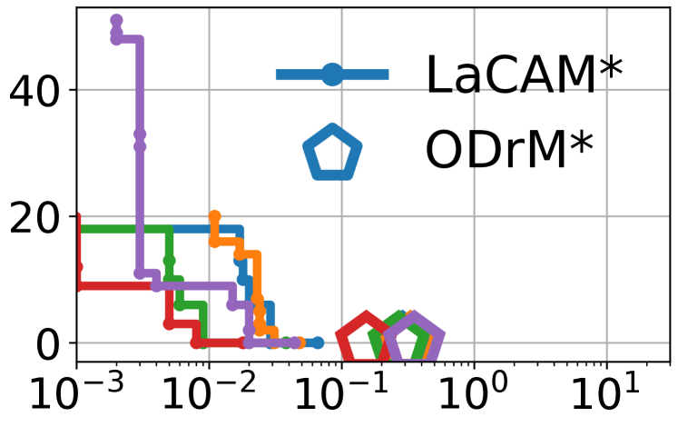
loss		loss
	time($\text{\,}\mathrm{ms}$)		time($\text{\,}\mathrm{ms}$)
	random-32-32-20, $|A|$$=$$30$		random-32-32-20, $|A|$$=$$100$
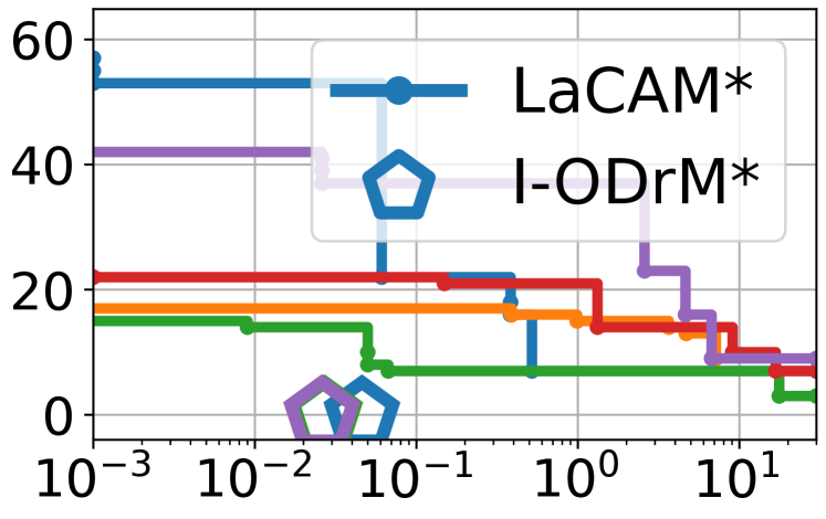
loss		loss
	time($\text{\,}\mathrm{ms}$)		time($\text{\,}\mathrm{ms}$)

Figure 7: Refinement of $\text{LaCAM}^{\ast}$. Three maps were used, shown in Tables 4 and 8. For each chart, five identical instances were used where starts and goals were set randomly. The optimization was for sum-of-loss. “loss” shows the gaps from scores of $\text{(I-)ODrM}^{\ast}$. In random-32-32-20, the bounded sub-optimal version with sub-optimality of 1.5 was used because $\text{ODrM}^{\ast}$ failed to solve the instances. $\text{LaCAM}^{\ast}$ used Alg. 2 as a configuration generator.

	tree	corners	tunnel	string	loop-chain	connector
no discard	10K	2M	410M	19M	N/A	N/A
w/Alg. 2	1K	28K	287K	103K	N/A	N/A
w/Alg. 4	1K	1K	199K	103K	N/A	N/A

Table 3: The number of search iterations for termination. “no discard” is blue-lines omitted version of $\text{LaCAM}^{\ast}$. The metric was for makespan. The instances are displayed in Table 4. In the last two instances, $\text{LaCAM}^{\ast}$ did not terminate before the timeout.

	tree		corners		tunnel		string		loop-chain		connector
unit of time: $\text{\,}\mathrm{ms}$
	time	s-opt	time	s-opt	time	s-opt	time	s-opt	time	s-opt	time	s-opt	solved
$\text{LaCAM}^{\ast}$	0	1.20	0	1.23	0	1.41	0	1.81	2	6.58	0	1.62	6/6
after $1\text{\,}\mathrm{s}$	0	1.00	2	1.00	6	1.00	7	1.00	578	1.35	226	1.00
$\text{A}^{\ast}$	0	1.00	0	1.00	30	1.00	27	1.00	11125	1.00	N/A	N/A	5/6
ODrM∗	5	1.00	2	1.00	396	1.00	402	1.00	N/A	N/A	N/A	N/A	4/6
I-ODrM∗	1	1.00	0	1.50	70	1.07	2	1.25	N/A	N/A	N/A	N/A	4/6
CBS	71	1.00	0	1.00	N/A	N/A	149	1.00	N/A	N/A	N/A	N/A	3/6
EECBS	2	1.00	1	1.00	N/A	N/A	0	1.00	N/A	N/A	N/A	N/A	3/6
OD	0	1.00	0	1.88	14	2.73	0	1.25	2133	31.22	5	1.50	6/6
LaCAM	0	1.17	1	2.12	92	2.00	0	2.25	55	17.83	0	1.56	6/6
PP	N/A	N/A	0	1.00	N/A	N/A	0	1.00	N/A	N/A	N/A	N/A	2/6
LNS2	N/A	N/A	0	1.00	N/A	N/A	0	1.00	N/A	N/A	29	1.00	3/6
PIBT	N/A	N/A	N/A	N/A	N/A	N/A	N/A	N/A	N/A	N/A	N/A	N/A	0/6
$\text{PIBT}^{+}$	0	3.50	0	1.25	0	4.07	0	2.12	N/A	N/A	0	1.81	5/6
BCP	194	-	150	-	N/A	-	117	-	N/A	-	N/A	-	3/6

Table 4: Results of the small complicated instances. “s-opt” is makespan normalized by optimal ones. The minimum is one. The sum-of-loss version appears in the appendix. Two rows show results of $\text{LaCAM}^{\ast}$: (i) scores for initial solutions and (ii) solution quality at $1\text{\,}\mathrm{s}$ and the runtime when that solution was obtained; they are an average of $10$ trials with different random seeds. Algorithms are categorized into $\text{LaCAM}^{\ast}$, those optimizing makespan, sub-optimal ones, and BCP optimizing another metric (i.e., flowtime).

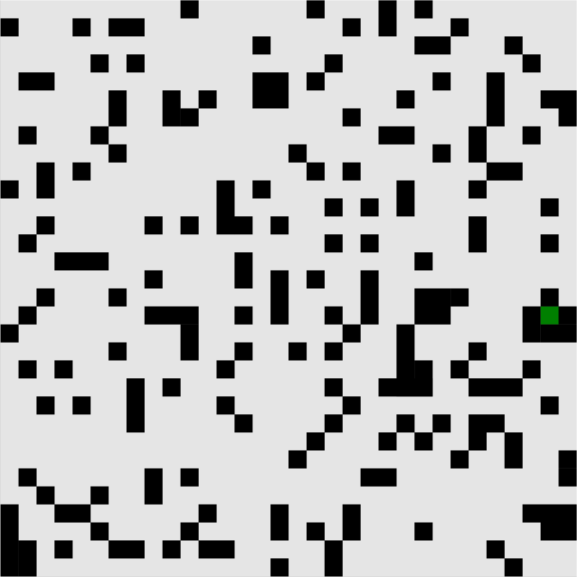
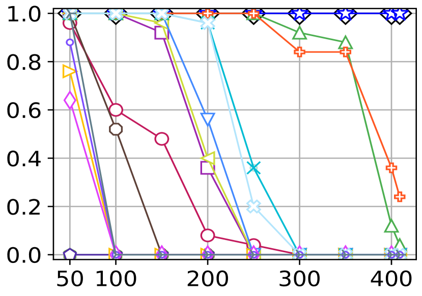
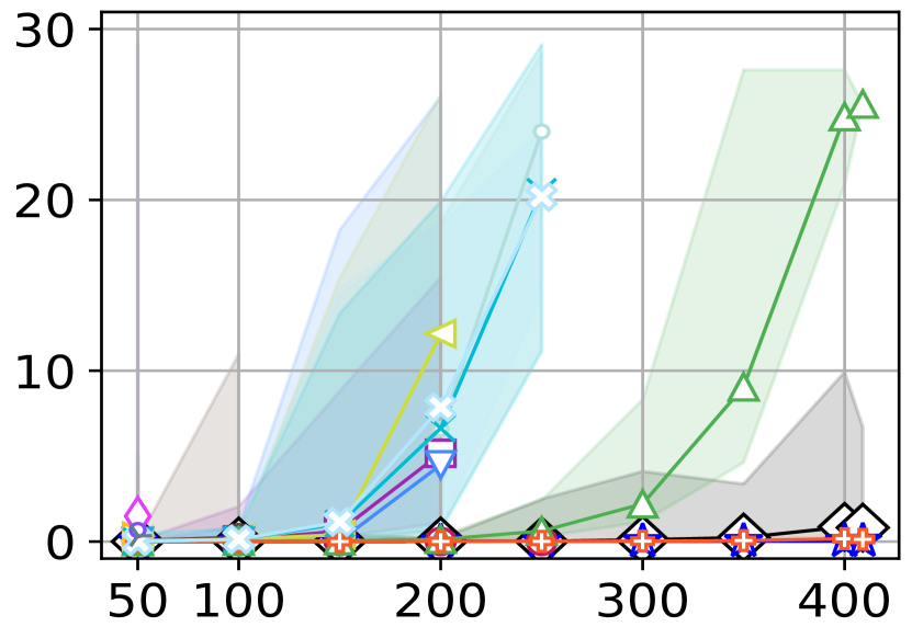
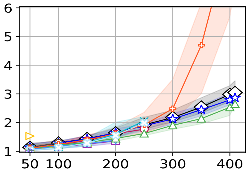
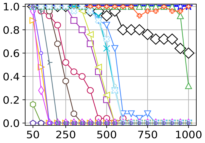
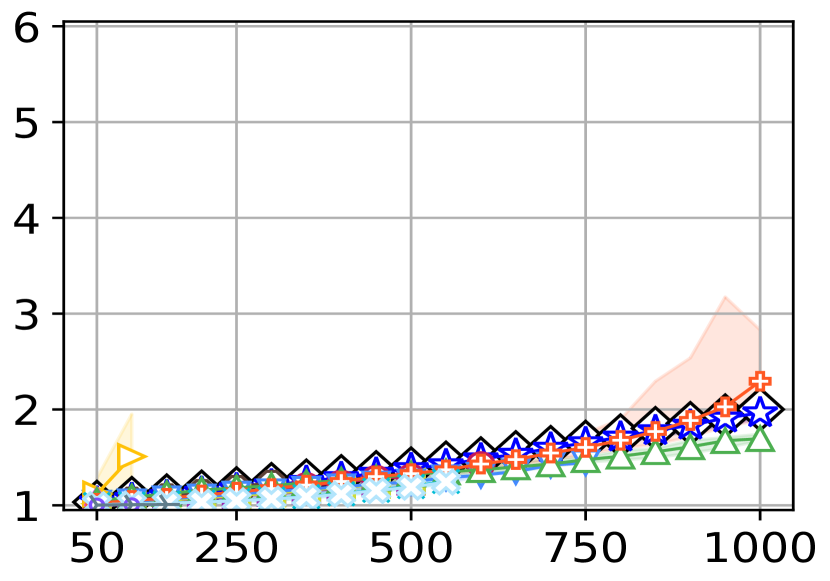
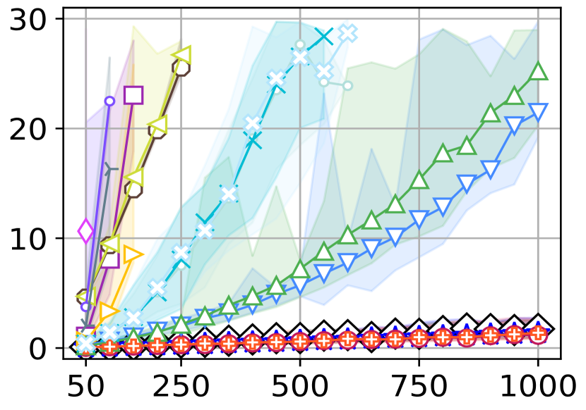
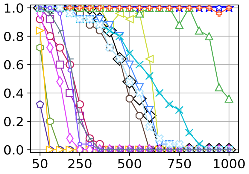
	random-32-32-20 32x32 ($|V|$$=$819)	random-64-64-20 64x64 ($|V|$$=$3,270)	brc202d 530x481 ($|V|$$=$43,151)	warehouse-20-40-10-2-1 321x123 ($|V|$$=$22,599)	maze-128-128-1 128x128 ($|V|$$=$8,191)
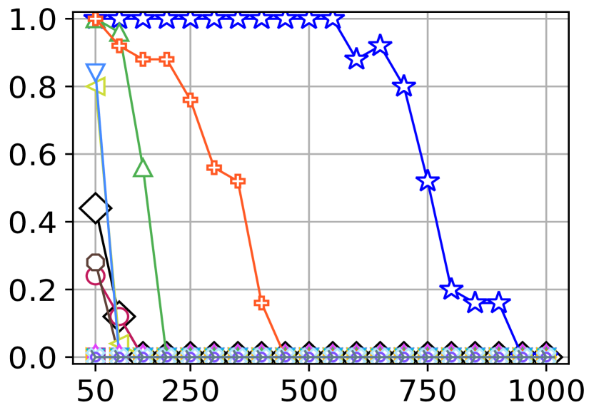
agents: $|A|$

Figure 8: Results of the MAPF benchmark. Scores of sum-of-loss are normalized by $\sum_{i\in A}\mathsf{dist}(s_{i},g_{i})$. For runtime and sum-of-loss, median, min, and max scores of solved instances within each solver are displayed. Scores of $\text{LaCAM}^{\ast}$ are from initial solutions.

Refinement of $\text{LaCAM}^{\ast}$.

Figure 7 shows how $\text{LaCAM}^{\ast}$ refines solutions. As baselines, we used scores of a complete and optimal algorithm called (I-)$\text{ODrM}^{\ast}$ Wagner and Choset (2015). In the small instances, $\text{LaCAM}^{\ast}$ quickly found initial solutions and converged to optimal ones. Meanwhile, the convergence speed was slow in large instances with many agents. This is due to finding new connections between known configurations becoming rare, hence reducing the chance of rewriting the search tree.

Effect of Discarding Redundant Nodes.

Table 3 shows how discarding redundant search nodes (blue lines of Alg. 3) affects the search to identify optimal solutions. Regardless of the generators, the discarding dramatically reduced the search effort. The reduction was larger with Alg. 4 because initial solutions can be found with smaller search iterations than Alg. 2. Note that without the discarding, the numbers of search iterations are equivalent between Alg. 2 and Alg. 4 because the search spaces are identical. In the remaining, $\text{LaCAM}^{\ast}$ uses Alg. 4 while LaCAM denotes the original implementation that uses Alg. 2.

Small Complicated Instances.

Table 4 shows the results of $\text{LaCAM}^{\ast}$ with instances retrieved from Luna and Bekris (2011). Overall, it immediately found not only initial solutions but also (near-)optimal ones. In contrast, the baselines failed some instances or returned low-quality solutions.

MAPF Benchmark.

We tested $\text{LaCAM}^{\ast}$ on the MAPF benchmark that includes 33 maps, each having 25 “random scenarios” which specify start-goal pairs. From each scenario, we extracted instances by increasing the number of agents by 50 up to the maximum (1,000 in most cases) and obtained 13,900 instances in total. The percentage of solved instances is summarized in Fig. 1. Figure 8 presents partial results for each map. $\text{LaCAM}^{\ast}$ only failed in the instances of maze-128-128-1 and sub-optimally solved all the other instances within $10\text{\,}\mathrm{s}$, outperforming the other algorithms. The failures might be reduced by improving the pattern detector; however, we consider such implementations are too optimized for the benchmark. As shown in Fig. 9, the refinement was steady but not dramatic due to the same reason of Fig. 7. Further discussions are available in the appendix.

Comparison with Anytime MAPF Solver.

We compared $\text{LaCAM}^{\ast}$ with AFS Cohen et al. (2018a), a CBS-based anytime MAPF solver that guarantees to converge optima. Table 5 summarizes the results. Contrary to $\text{LaCAM}^{\ast}$, AFS can obtain plausible solutions from the beginning, however, it compromises scalability. We consider this quality gap can be overcome by developing better generators other than PIBT.

Extremely Dense Scenarios.

Table 6 reports $\text{LaCAM}^{\ast}$ in very congested scenarios that existing solvers mostly fail. Even with such challenging cases, $\text{LaCAM}^{\ast}$ solved many instances, demonstrating its excellent scalability.

6 Conclusion and Discussion

The primary challenge of MAPF is to maintain solvability and solution quality while suppressing planning efforts. To break this tradeoff, this paper presented two enhancements to LaCAM, namely, $\text{LaCAM}^{\ast}$ which eventually converges to optima and an effective configuration generator. The enhancements were thoroughly assessed, achieving remarkable results. From the empirical evidence, we believe that $\text{LaCAM}^{\ast}$ has developed a new frontier in MAPF.

Related Work.

LaCAM^(∗) relates to partial successor expansion during the search, as seen in Goldenberg et al. (2014); Wagner and Choset (2015), because it also generates a subset of successors, but differs in the use of constraints and a configuration generator. Anytime MAPF algorithms that converge to optima have been studied Standley and Korf (2011); Cohen et al. (2018a); Vedder and Biswas (2021). However, their scalability is limited; they often fail to derive initial solutions, as we empirically saw. Techniques to refine arbitrary MAPF solutions have also been studied Surynek (2013); De Wilde et al. (2014); Okumura et al. (2021); Li et al. (2021a) but they do not ensure optimality. Rewriting the search tree structure is popular in optimal motion planning Karaman and Frazzoli (2011); Shome et al. (2020), by which $\text{LaCAM}^{\ast}$ is partially inspired. Incorporating swap into PIBT is inspired by sub-optimal rule-based MAPF algorithms Luna and Bekris (2011); De Wilde et al. (2014). Meanwhile, the solution quality of rule-based approaches themselves is often severely compromised.

Future Directions.

We are interested in more effective configuration generators than PIBT variants which can output near-optimal initial solutions. Improving the convergence speed of $\text{LaCAM}^{\ast}$ is also important. Moreover, $\text{LaCAM}^{\ast}$ in MAPF variants, e.g., multi-robot motion planning Okumura and Défago (2023), is worth to be studied. Other than MAPF, since $\text{LaCAM}^{\ast}$ is just a graph pathfinding algorithm, applying its concept to other planning domains might be exciting.

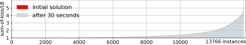
Figure 9: Refinement by $\text{LaCAM}^{\ast}$ for the MAPF benchmark. On the x-axis, the figure sorts 13,766 solved instances out of 13,900 by initial solution quality and displays the scores in red bars. For each instance, we also plot the solution quality at 30 seconds using gray bars. Hence, the effect of refinement is visualized by tiny red areas.

	solved(%)		time-init($\text{\,}\mathrm{ms}$)		loss-init		loss-$30\text{\,}\mathrm{s}$
$|A|$	AFS	$\text{LaCAM}^{\ast}$	AFS	$\text{LaCAM}^{\ast}$	AFS	$\text{LaCAM}^{\ast}$	AFS	$\text{LaCAM}^{\ast}$
50	100	100	88	1	25	159	24	118
100	56	100	7223	2	140	609	139	545
150	0	100	N/A	4	N/A	1463	N/A	1368

Table 5: Comparison of anytime MAPF algorithms. We used sum-of-loss and 25 “random” scenarios of random-32-32-20. “init” shows scores related to initial solutions. “loss” is the gap scores from $\sum_{i\in A}\mathsf{dist}(s_{i},g_{i})$. The scores are averaged for instances solved by both solvers, except for $|A|=150$ because AFS failed all.

map	$|A|$	%	time($\text{\,}\mathrm{s}$)	other algorithms
empty-8-8	58	100	0.00	PIBT&LaCAM (100%; $0.00\text{\,}\mathrm{s}$)
random-32-32-20	737	100	0.63	LaCAM (4%; $14.81\text{\,}\mathrm{s}$)
random-64-64-20	2943	68	11.64	N/A
maze-128-128-10	9772	100	55.54	N/A

Table 6: Results on extremely dense scenarios. $|A|$ was adjusted so that $|A|/|V|=0.9$. For each scenario, 25 instances were prepared while randomly placing starts and goals. “%” is the success percentage by $\text{LaCAM}^{\ast}$ with timeout of $60\text{\,}\mathrm{s}$. “time” is the median runtime to obtain initial solutions. We also tested the other solvers in Fig. 1 and report solvers that solved in at least one instance.

Appendix

Appendix A MAPF-Specific Part of LaCAM

Algorithm 5 presents the full version of LaCAM (Alg. 1). To highlight differences, the pseudocode uses gray-out for the same lines with Alg. 1. In what follows, we complement the MAPF-specific part of Alg. 5.

Constraint.

Recall that a constraint in LaCAM is defined by each domain. In MAPF, a constraint specifies which agent is where in the next configuration. Then, a node $\mathcal{C}$ in the constraint tree specifies locations for multiple agents in the next configuration. The configuration generator must follow this specification.

Constraint Generation.

To determine which agent will be constrained, a high-level node $\mathcal{N}$ includes $\mathit{order}$, an enumeration of all agents sorted by specific criteria. This is specified by two functions: $\mathsf{get\_init\_order}$ (5) and $\mathsf{get\_order}$ (20). An agent $i$ is then selected following $\mathit{order}$ and depth of the low-level node in the constraint tree, which is obtained by the function $\mathsf{depth}$ (14). Doing so ensures that each path of the constraint tree has no duplicate agents. Constraints are generated for all possible locations from $\mathcal{N}.\mathit{config}[i]$ (Lines 14–16). The constraint tree is not developed when the depth of the low-level node equals $|A|$ (12) because all agents have constraints in such a node.

Appendix B Evaluation

B.1 Baselines

We tested a variety of representative or state-of-the-art MAPF algorithms that have diverse properties for solvability and optimality as follows. See also Fig. 1.

• $\text{A}^{\ast}$ Hart et al. [1968] as a vanilla search algorithm. It is complete and optimal. The used objectives were makespan ($\text{A}^{\ast}$-m) and sum-of-loss ($\text{A}^{\ast}$-l).

• $\text{A}^{\ast}$ with operator decomposition (OD) Standley [2010] as an adaptation of the general search to MAPF. It was implemented as a greedy best-first search to obtain solutions as much as possible. The heuristic was the sum of distance toward goals.

• ODrM^∗ Wagner and Choset [2015] as a state-of-the-art optimal and complete algorithm, similar to $\text{A}^{\ast}$. The used objectives were sum-of-loss (ODrM^∗-l) and makespan (ODrM^∗-m). The implementation was from https://github.com/gswagner/mstar_public. The original implementation uses sum-of-loss as an objective function. The makespan version was adapted from it.

• Inflated ODrM^∗ (I-ODrM^∗) Wagner and Choset [2015] as a state-of-the-art bounded sub-optimal and complete algorithm, which is a variant of ODrM^∗. The used objective is makespan (I-ODrM^∗-m) and sum-of-loss (I-ODrM^∗-l). The sub-optimality was set to five to find solutions as much as possible.

• BCP Lam et al. [2022] as a state-of-the-art optimal solver that uses reduction to a mathematical optimization problem. BCP is solution complete, namely, it cannot distinguish unsolvable instances. The implementation used CPLEX for mathematical optimization and was retrieved from https://github.com/ed-lam/bcp-mapf. The used objective was flowtime (aka. sum-of-costs), following the authors’ implementation.

• CBS Sharon et al. [2015] with many improvement techniques as appeared in Li et al. [2021b], as a state-of-the-art optimal solver. This is representative of two-level combinatorial search. CBS is solution complete. The implementation was retrieved from https://github.com/Jiaoyang-Li/CBSH2-RTC. The used objectives were flowtime (CBS-f), makespan (CBS-m), and sum-of-loss (CBS-l). The original implementation uses flowtime as an objective function. The makespan and sum-of-loss versions were adapted from it.

• EECBS Li et al. [2021c] as a state-of-the-art bounded sub-optimal but solution complete algorithm, which is a variant of CBS. The used objectives were flowtime (EECBS-f), makespan (EECBS-m), and sum-of-loss (EECBS-l). The sub-optimality was set to five. The implementation was retrieved from https://github.com/Jiaoyang-Li/EECBS. The original implementation uses flowtime as an objective function. The makespan and sum-of-loss versions were adapted from it.

  Algorithm 5 LaCAM

  1:

  2:

  3:

  4: initialize $\mathit{Open}$, $\mathit{Explored}$ $\triangleright$ stack, hash table

  5: ${\color[rgb]{0.6,0.6,0.6}\mathcal{N}^{\text{init}}\leftarrow}\begin{aligned} {\color[rgb]{0.6,0.6,0.6}\bigl{\langle}}~{}&{\color[rgb]{0.6,0.6,0.6}\mathit{config}:\mathcal{S},\mathit{tree}:\llbracket~{}\mathcal{C}^{\text{init}}~{}\rrbracket,\mathit{parent}:\bot,}\\ &\mathit{order}:\mathsf{get\_init\_order}()~{}{\color[rgb]{0.6,0.6,0.6}\bigr{\rangle}}\end{aligned}$

  6: $\mathit{Open}.\mathsf{push}\left(\mathcal{N}^{\text{init}}\right)$;  $\mathit{Explored}[\mathcal{S}]=\mathcal{N}^{\text{init}}$

  7: while $\mathit{Open}\neq\emptyset$ do

  8:    $\mathcal{N}\leftarrow\mathit{Open}.\mathsf{top}()$

  9:    if $\mathcal{N}.\mathit{config}=\mathcal{G}$ then return $\mathsf{backtrack}(\mathcal{N})$

  10:    if $\mathcal{N}.\mathit{tree}=\emptyset$ then $\mathit{Open}.\mathsf{pop}()$; continue

  11:    $\mathcal{C}\leftarrow\mathcal{N}.\mathit{tree}.\mathsf{pop}()$

  12:    if $0pt(\mathcal{C})\leq|A|$ then $\triangleright$ $\mathsf{low\_level\_expansion}$

  13:       $i\leftarrow\mathcal{N}.\mathit{order}\left[0pt(\mathcal{C})\right]$

  14:       for $u\in\mathsf{neigh}(\mathcal{N}.\mathit{config}[i])\cup\left\{\mathcal{N}.\mathit{config}[i]\right\}$ do

  15:          $\mathcal{C}^{\text{new}}\leftarrow\langle~{}\mathit{parent}:\mathcal{C},\mathit{who}:i,\mathit{where}:u~{}\rangle$

  16:          $\mathcal{N}.\mathit{tree}.\mathsf{push}\left(\mathcal{C}^{\text{new}}\right)$           

  17:    $\mathcal{Q}^{\text{new}}\leftarrow\mathsf{configuration\_generator}(\mathcal{N},\mathcal{C})$

  18:    if $\mathcal{Q}^{\text{new}}=\bot$ then continue

  19:    if $\mathit{Explored}\left[\mathcal{Q}^{\text{new}}\right]\neq\bot$ then continue

  20:    ${\color[rgb]{0.6,0.6,0.6}\mathcal{N}^{\text{new}}\leftarrow}\begin{aligned} {\color[rgb]{0.6,0.6,0.6}\langle}~{}&{\color[rgb]{0.6,0.6,0.6}\mathit{config}:\mathcal{Q}^{\text{new}},\mathit{tree}:\left\llbracket~{}\mathcal{C}^{\text{init}}~{}\right\rrbracket,\mathit{parent}:\mathcal{N},}\\ &\mathit{order}:\mathsf{get\_order}(\mathcal{Q}^{\text{new}},\mathcal{N})~{}{\color[rgb]{0.6,0.6,0.6}\bigr{\rangle}}\end{aligned}$

  21:    $\mathit{Open}.\mathsf{push}\left(\mathcal{N}^{\text{new}}\right)$; $\mathit{Explored}\left[\mathcal{Q}^{\text{new}}\right]=\mathcal{N}^{\text{new}}$

  22: return NO_SOLUTION

• Prioritized planning (PP) Erdmann and Lozano-Perez [1987]; Silver [2005] as a basic approach for MAPF. The implementation first uses a distance heuristic Van Den Berg and Overmars [2005] for the planning order. Furthermore, it involves the repetition of PP with random priorities until the problem is solved. The implementation was adapted from https://github.com/Kei18/pibt2.

• MAPF-LNS2 (LNS2) Li et al. [2022] as a state-of-the-art sub-optimal and incomplete solver, based on a large neighborhood search. The implementation was retrieved from https://github.com/Jiaoyang-Li/MAPF-LNS2.

• PIBT Okumura et al. [2022], which is an incomplete and sub-optimal algorithm. A vanilla PIBT was tested because LaCAM used PIBT. To detect planning failure, PIBT was regarded as a failure when it reached pre-defined sufficiently large timesteps. The implementation was retrieved from https://github.com/Kei18/pibt2.

• $\text{PIBT}^{+}$ Okumura et al. [2022], as a state-of-the-art scalable MAPF solver, which is incomplete and sub-optimal. It used push and swap Luna and Bekris [2011] to complement solutions.

• LaCAM Okumura [2023], on which $\text{LaCAM}^{\ast}$ is based. This is a complete sub-optimal algorithm. It used a vanilla PIBT as a configuration generator. The implementation was from https://github.com/Kei18/lacam.

• AFS Cohen et al. [2018a], an anytime version of CBS that eventually converges to optima. Its implementation was obtained from the authors of the paper. The original implementation uses flowtime as an objective function. The sum-of-loss versions were adapted from it.

B.2 Small Complicated Instances for Sum-of-loss

Table 7 presents the results of the small complicated instances for the sum-of-loss, corresponding to Table 4. Overall, the results are similar to those for makespan; many solvers failed in some instances or compromised the solution quality, while $\text{LaCAM}^{\ast}$ immediately found initial solutions and converged to (near-)optimal solutions.

B.3 MAPF Benchmark

How to Test Each Algorithm.

When increasing the number of agents by $50$, we stopped testing some algorithms if they failed to solve all instances in the previous round.

Results.

Figures 10, 11 and 12 present full results of the MAPF benchmark, complementing Fig. 8. In addition to sum-of-loss, we also present makespan normalized by $\max_{i\in A}\mathsf{dist}(s_{i},g_{i})$. Scores of $\text{LaCAM}^{\ast}$ are for initial solutions. Overall, $\text{LaCAM}^{\ast}$ solved a variety of problem instances that have diverse sizes of graphs or agents, sparseness, and complexity, within several seconds. Solution qualities of $\text{LaCAM}^{\ast}$ are comparable to other sub-optimal algorithms. Specifically, the qualities are similar to those of PIBT and LaCAM because it is based on these algorithms.

Discussion of Other Algorithms.

Although recent remarkable progress in MAPF studies, the scalability of optimal algorithms (e.g., $\text{ODrM}^{\ast}$, BCP, CBS) is limited; they failed to handle a few hundred agents in most cases. Bounded sub-optimal algorithms such as $\text{I-ODrM}^{\ast}$ and EECBS can solve a variety of instances but struggle to solve challenging instances (e.g., with 1000 agents). Sub-optimal algorithms such as PP, LNS2, or PIBT⁽⁺⁾ sometimes can handle such challenging instances but still failed many instances. From another perspective, it is ideal for an algorithm to be complete, however, the completeness can be the bottleneck for achieving speed. This is observed in $\text{A}^{\ast}$, OD, and $\text{ODrM}^{\ast}$.

In general, makespan-optimal solutions are easier to obtain than sum-of-loss-optimal ones. This is because, given an instance, the number of makespan-optimal solutions is larger than that of sum-of-loss. Empirically, this is validated with $\text{ODrM}^{\ast}$ and CBS in Fig. 1. For instance, CBS-m solved much more instances than CBS-l. Meanwhile, we can see a reverse trend in $\text{I-ODrM}^{\ast}$, which is a bounded sub-optimal complete algorithm; $\text{I-ODrM}^{\ast}$-l solved more instances than $\text{I-ODrM}^{\ast}$-m. We regard this as an effect of admissible heuristics. The sum-of-loss optimization uses $\sum_{i\in A}\mathsf{dist}(s_{i},g_{i})$ while the makespan optimization uses $\max_{i\in A}\mathsf{dist}(s_{i},g_{i})$; the former provides more informatic guidance than the latter.

	tree		corners		tunnel		string		loop-chain		connector
	time	s-opt	time	s-opt	time	s-opt	time	s-opt	time	s-opt	time	s-opt	solved
$\text{LaCAM}^{\ast}$	0	1.25	0	1.12	0	1.46	0	2.36	2	7.12	0	(1.48)	6/6
after $1\text{\,}\mathrm{s}$	0	1.00	13	1.00	77	1.00	8	1.00	700	1.44	408	(1.08)
$\text{A}^{\ast}$	0	1.00	149	1.00	35	1.00	25	1.00	15124	1.00	N/A	N/A	5/6
ODrM∗	3	1.00	40	1.00	675	1.00	0	1.00	N/A	N/A	N/A	N/A	4/6
I-ODrM∗	0	1.00	0	1.31	257	1.08	0	1.00	N/A	N/A	124	(1.39)	5/6
CBS	70	1.00	0	1.00	N/A	N/A	180	1.00	N/A	N/A	N/A	N/A	3/6
EECBS	2	1.00	0	1.00	N/A	N/A	0	1.00	N/A	N/A	86	(1.61)	4/6
OD	0	1.00	0	1.50	14	2.57	0	1.20	2133	30.62	5	(1.38)	6/6
LaCAM	0	1.23	1	1.69	92	1.91	0	3.30	55	19.15	0	(1.45)	6/6
PP	N/A	N/A	0	1.00	N/A	N/A	0	1.00	N/A	N/A	N/A	N/A	2/6
LNS2	N/A	N/A	0	1.00	N/A	N/A	0	1.00	N/A	N/A	29	(1.00)	3/6
PIBT	N/A	N/A	N/A	N/A	N/A	N/A	N/A	N/A	N/A	N/A	N/A	N/A	0/6
$\text{PIBT}^{+}$	0	4.38	0	1.12	0	3.91	0	2.20	N/A	N/A	0	(1.68)	5/6
BCP	194	-	150	-	N/A	-	117	-	N/A	-	N/A	-	3/6

Table 7: Results of the small complicated instances for sum-of-loss. The time of the unit is $\text{\,}\mathrm{ms}$. See also the caption of Table 4. Regarding sum-of-loss in connector (decorated by parentheses), the scores normalized by known best values (80) are presented due to failing to obtain the optimal scores.

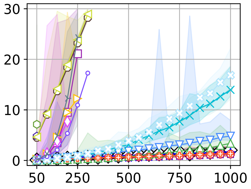
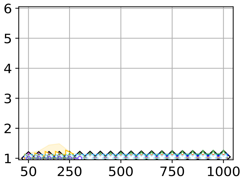
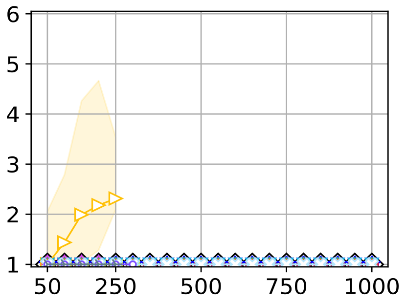
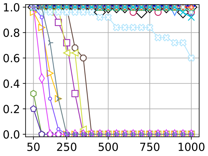
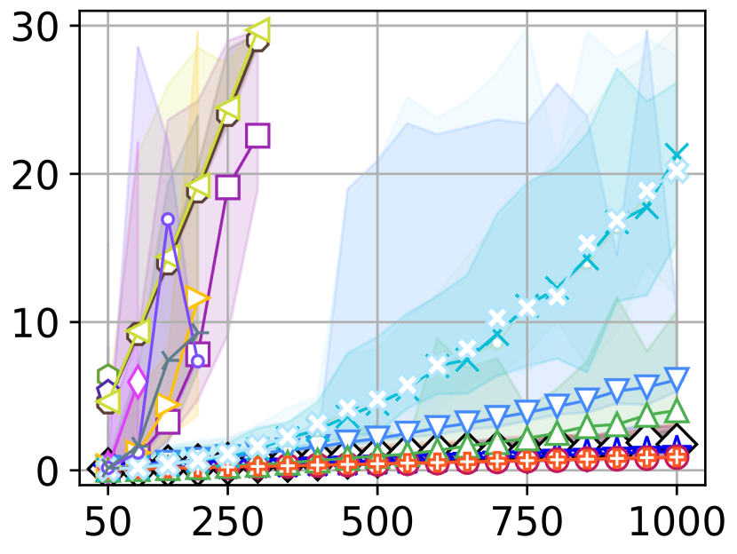
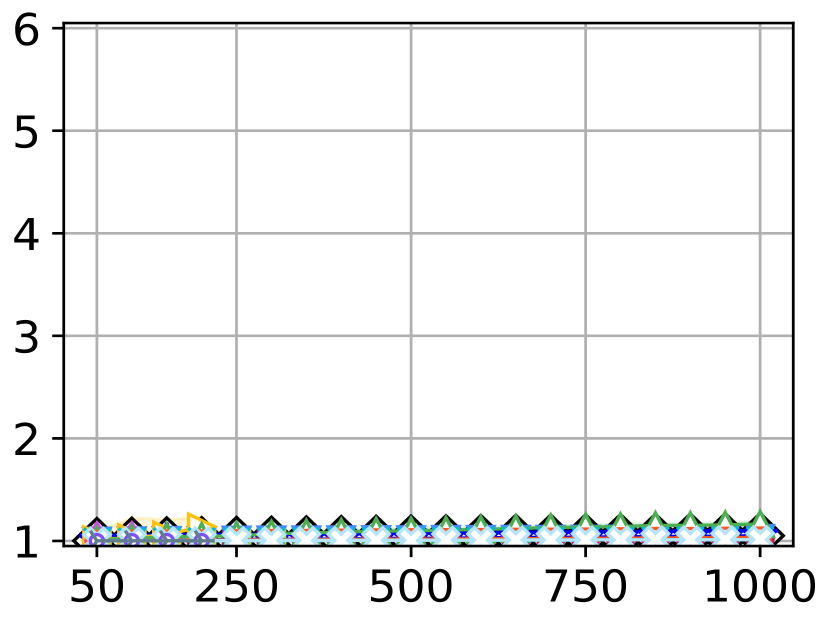
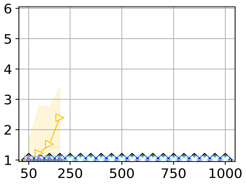
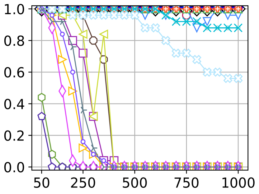
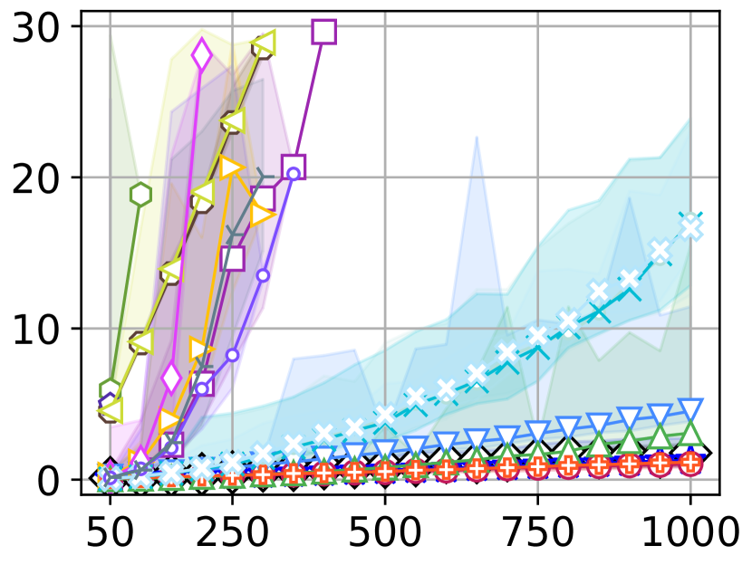
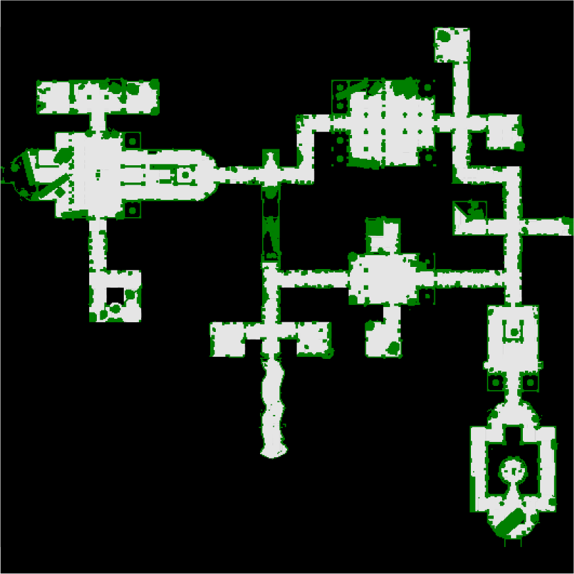
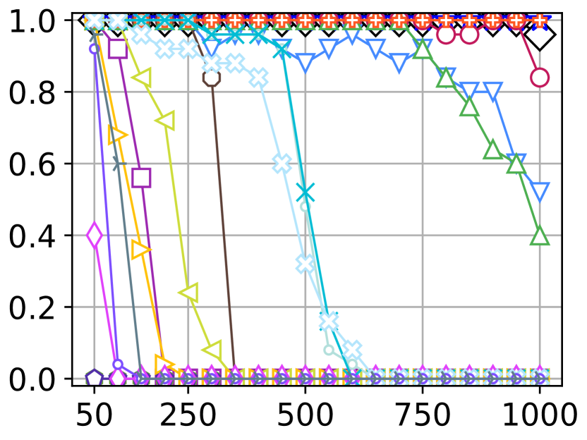
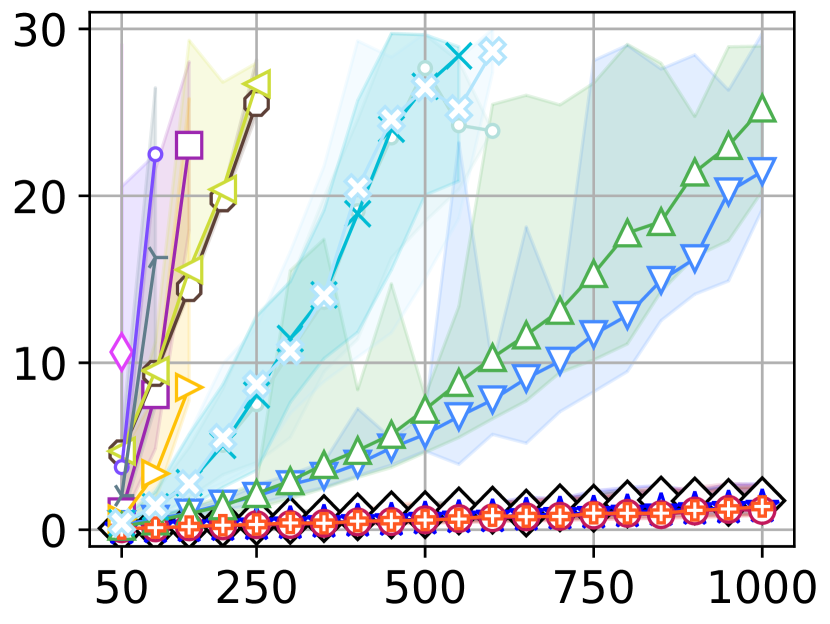
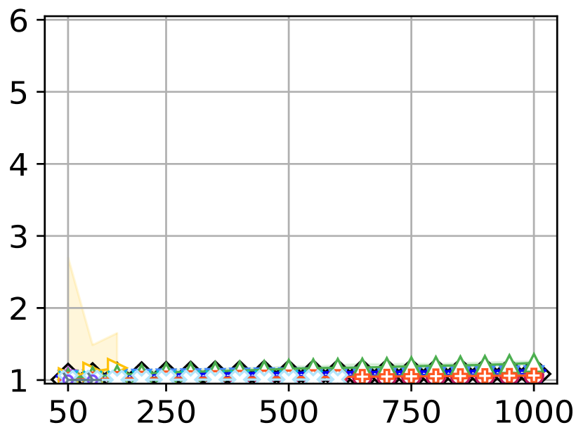
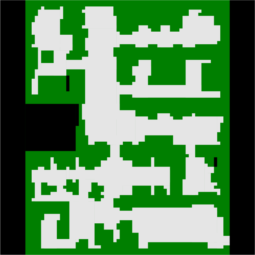
	Berlin_1_256 256x256 (47,540)	Boston_0_256 256x256 (47,768)	Paris_1_256 256x256 (47,240)	brc202d 530x481 (43,151)	den312d 65x81 (2,445)	den520d 256x257 (28,178)
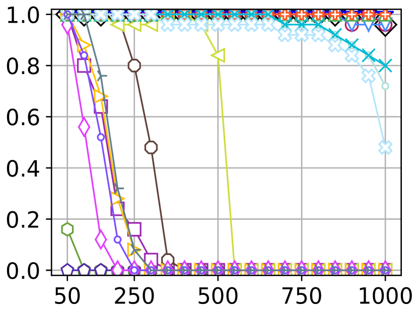
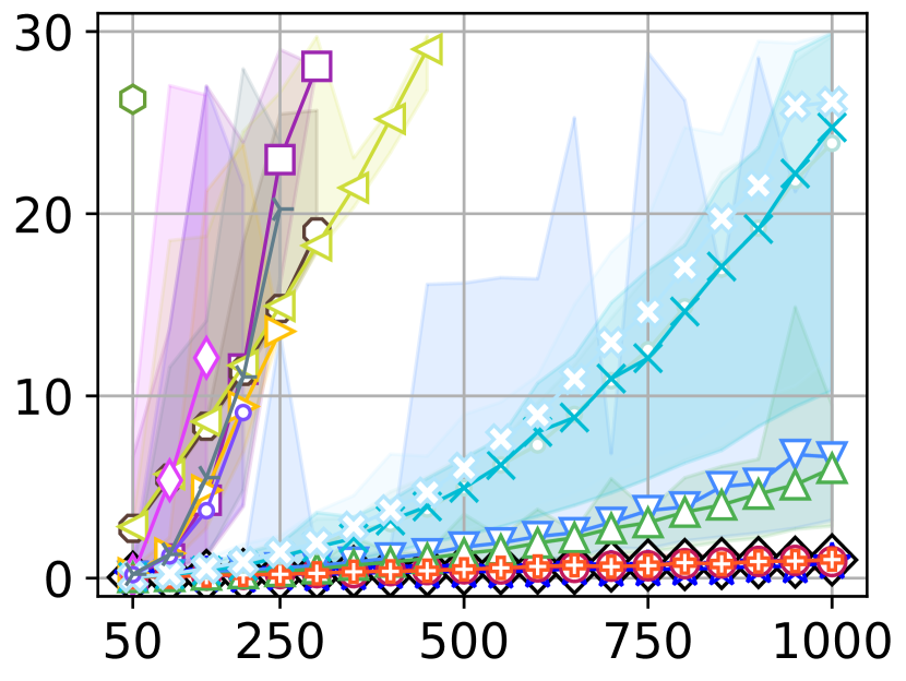
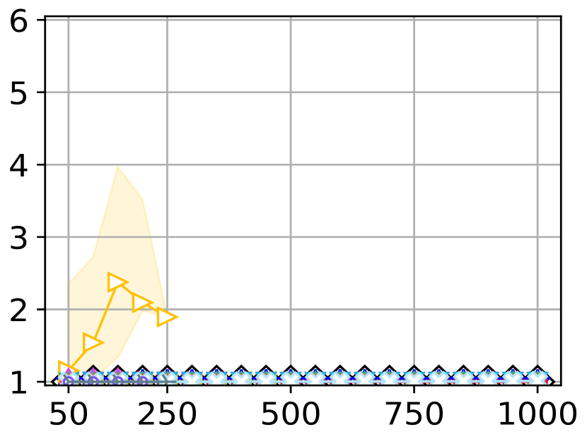
agents: $|A|$
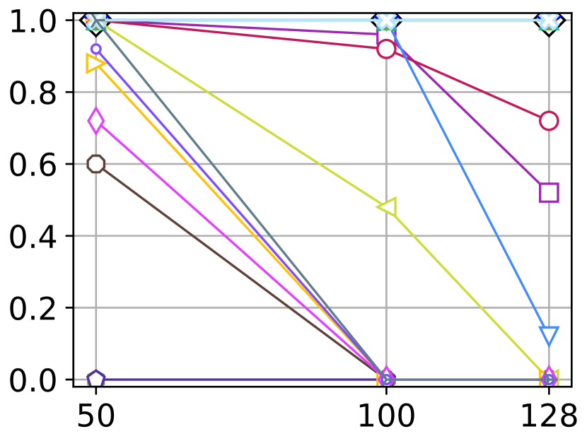
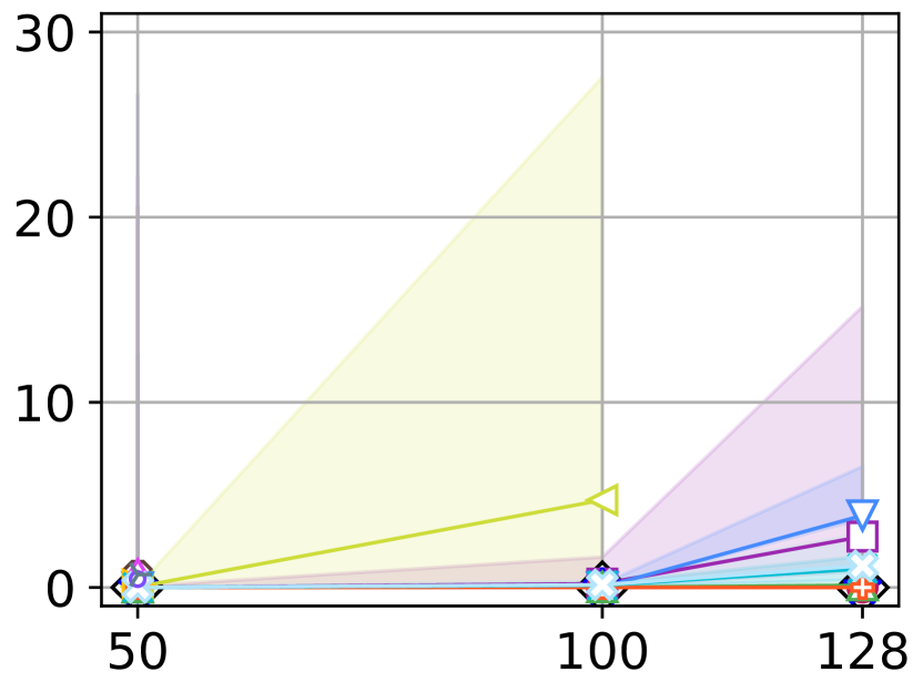
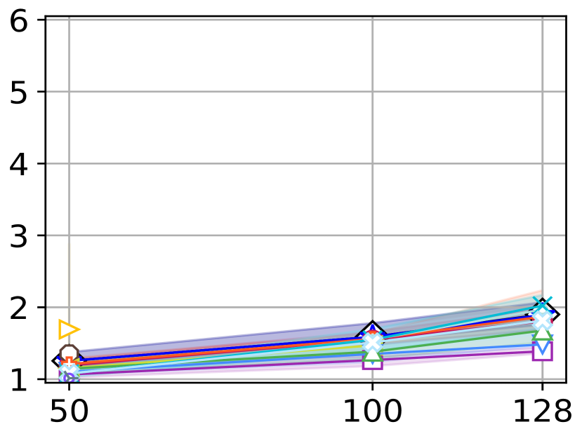
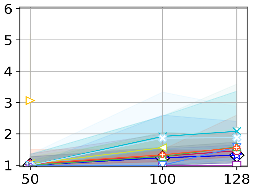
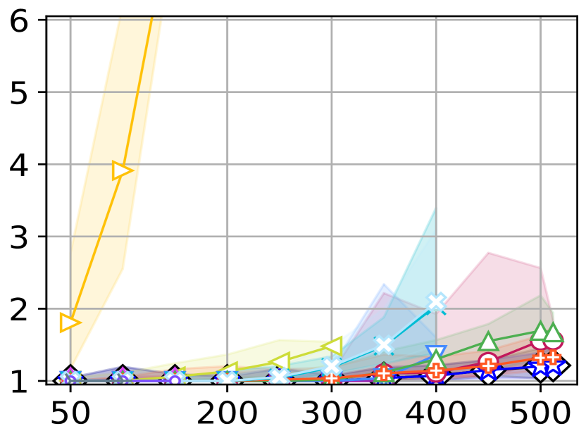
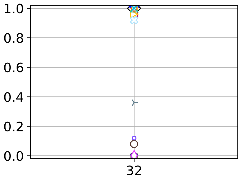
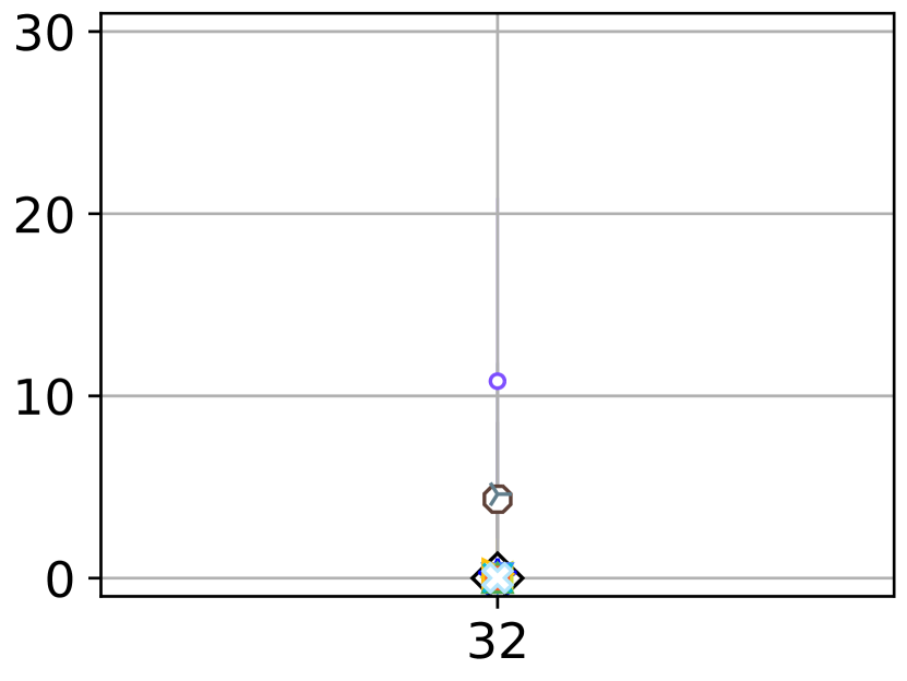
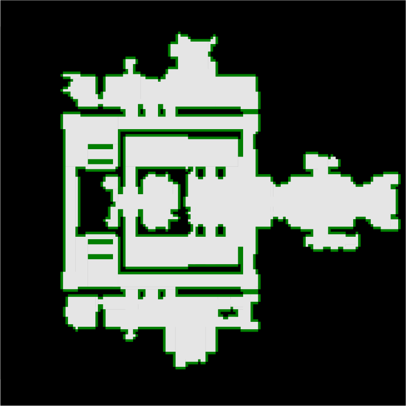
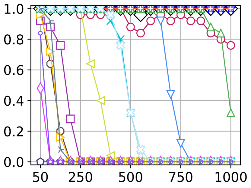
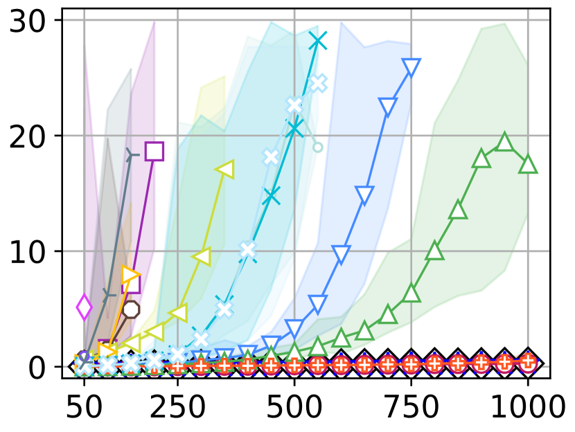
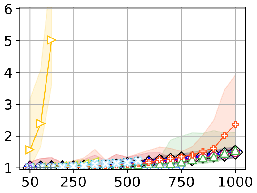
	empty-16-16 16x16 (256)	empty-32-32 32x32 (1,024)	empty-48-48 48x48 (2,304)	empty-8-8 8x8 (64)	ht_chantry 162x141 (7,461)	ht_mansion_n 133x270 (8,959)
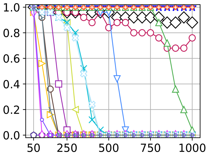
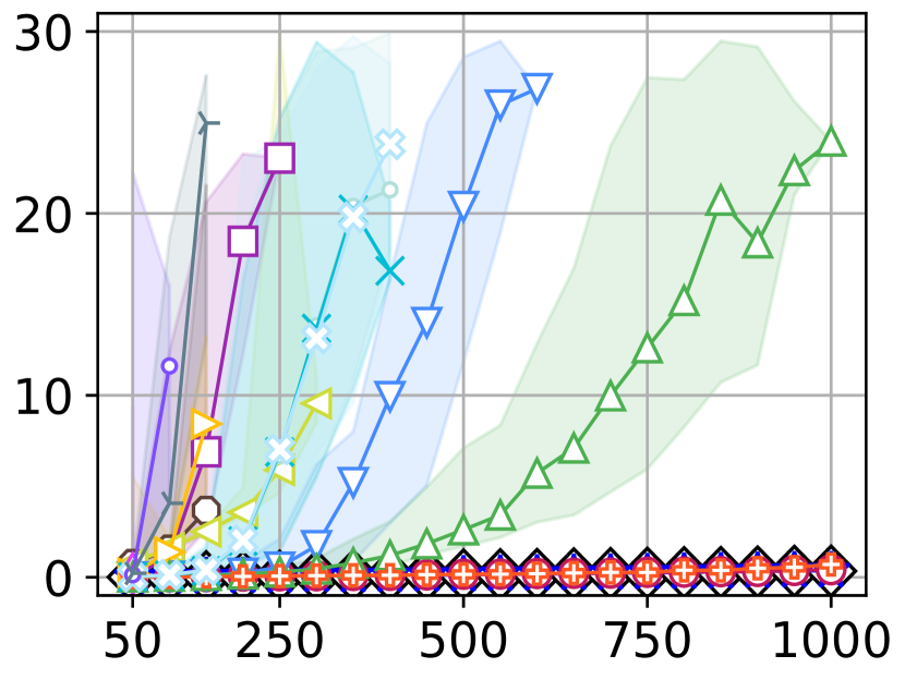
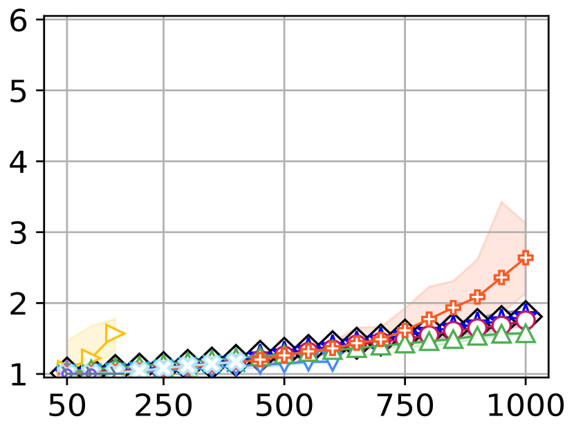
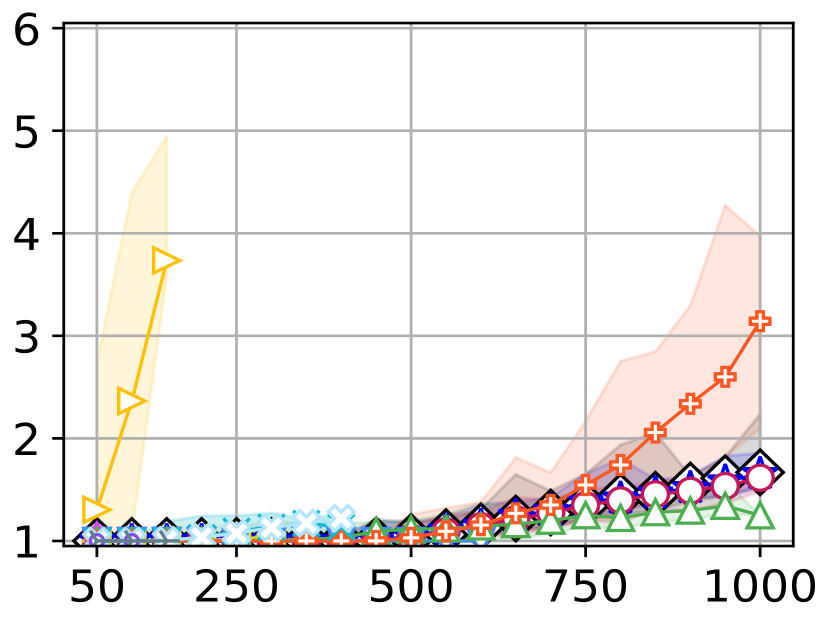
agents: $|A|$

Figure 10: Result of the MAPF benchmark (1/3). See also the caption of Fig. 8. $|V|$ is shown in parentheses.

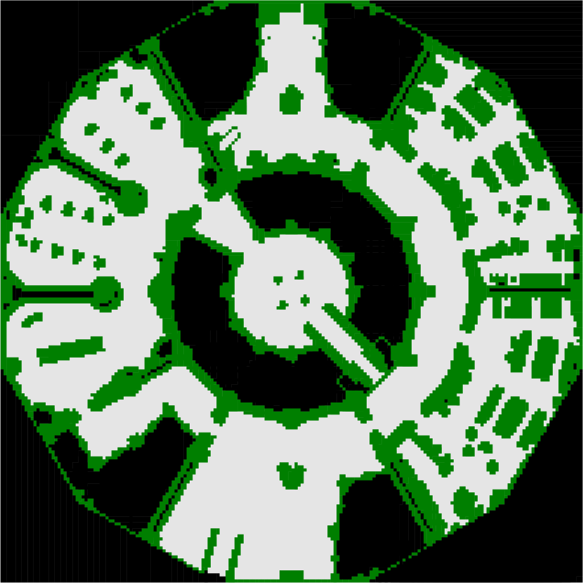
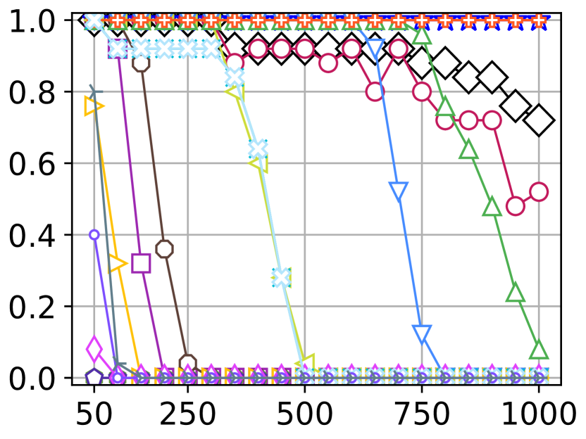
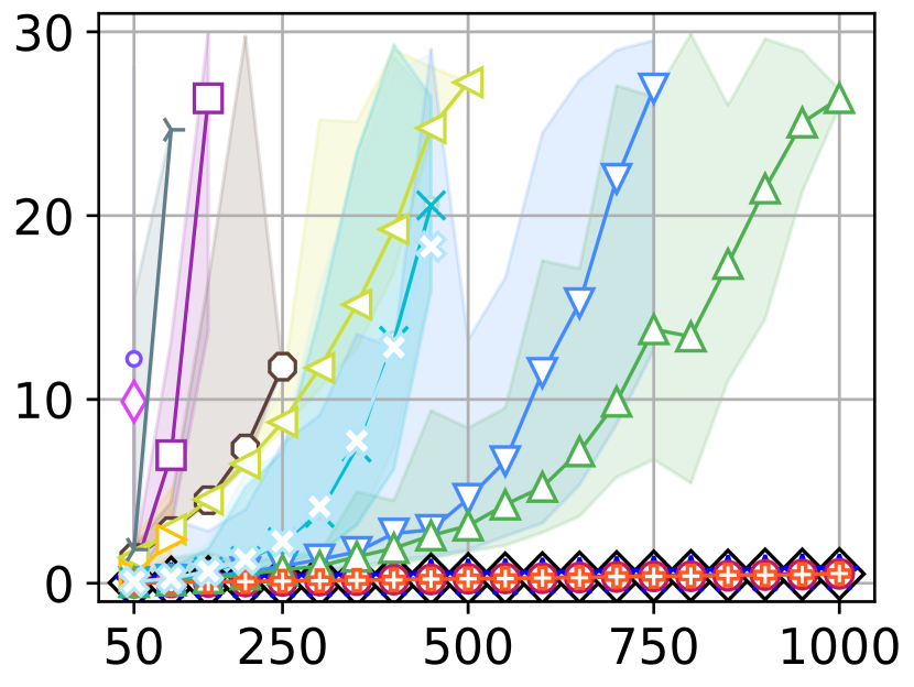
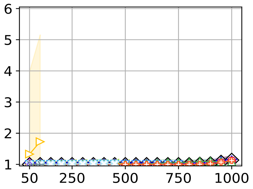
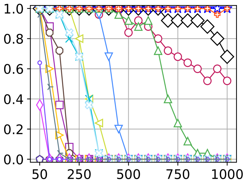
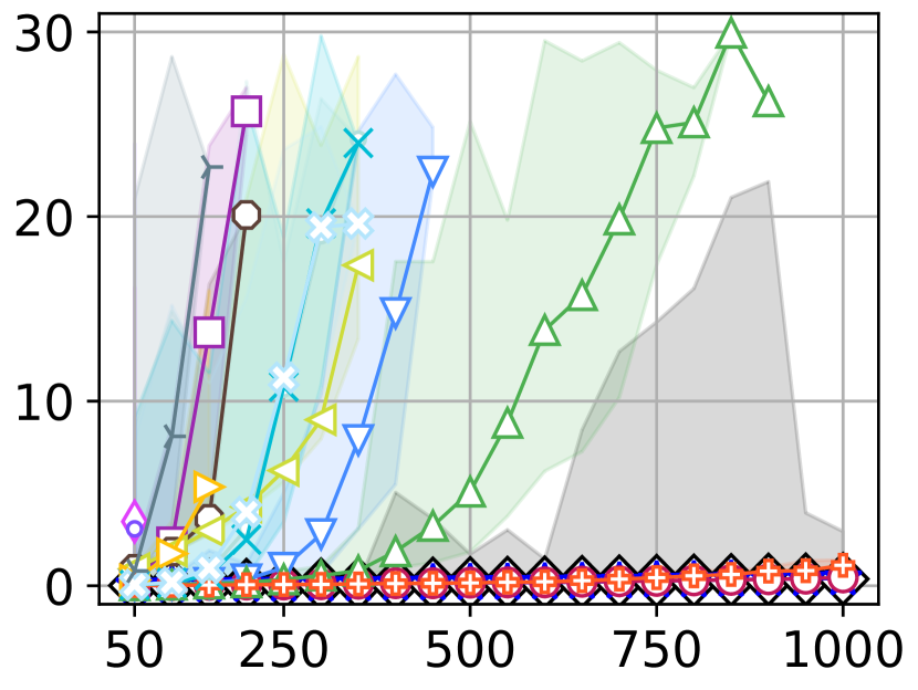
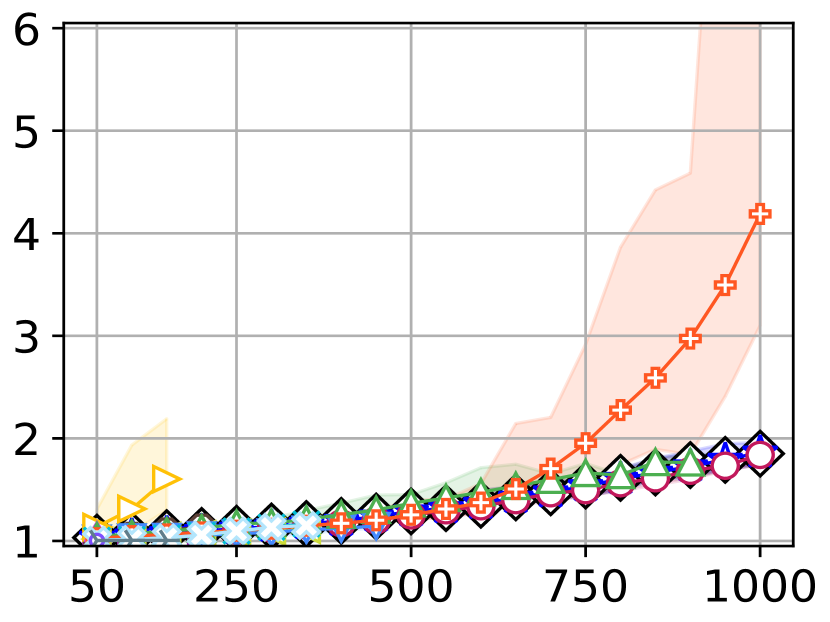
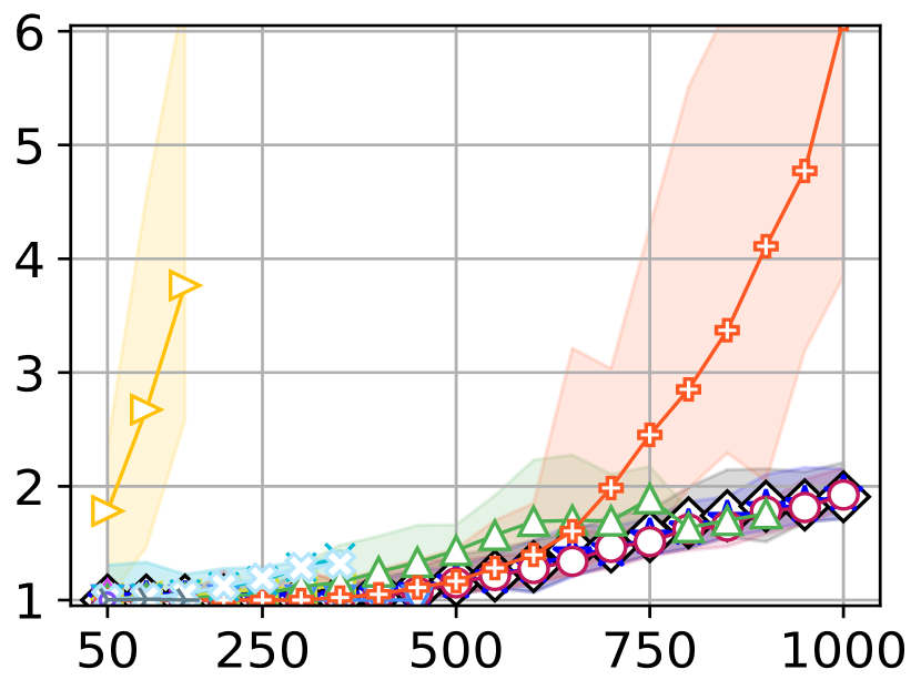
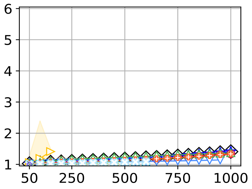
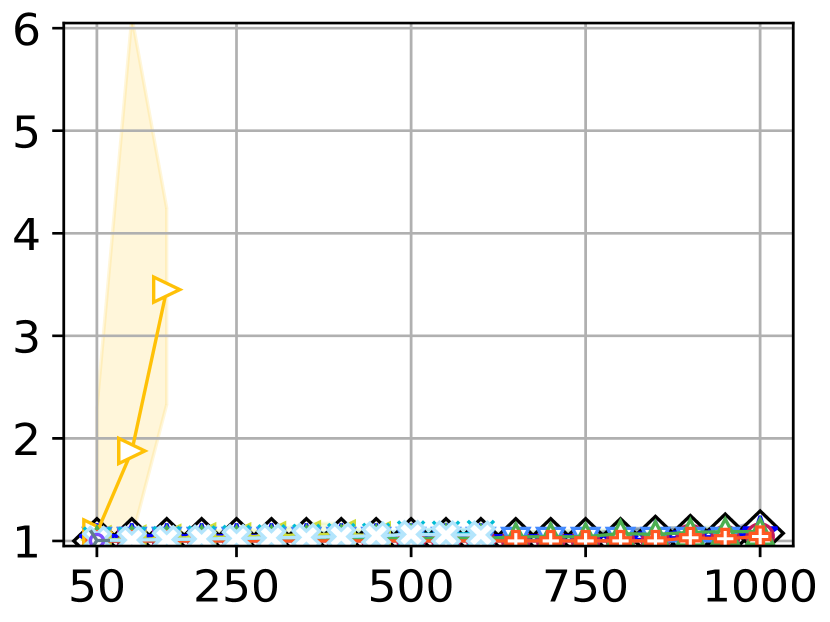
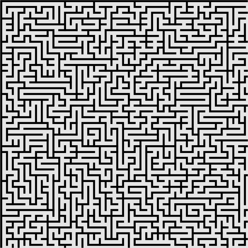
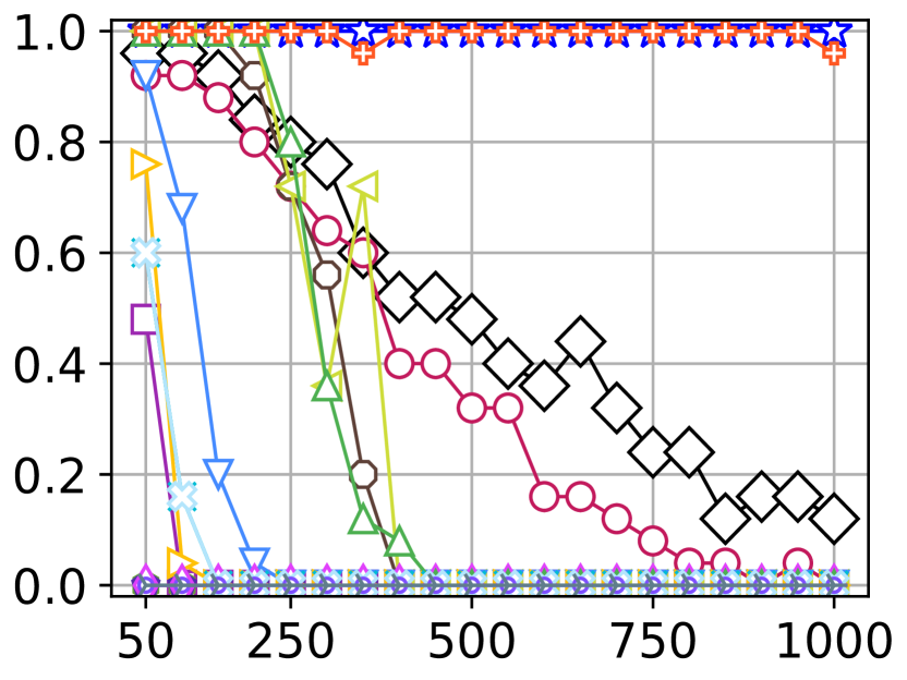
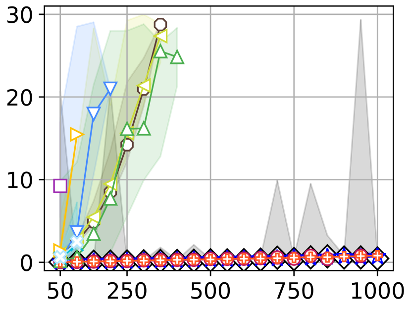
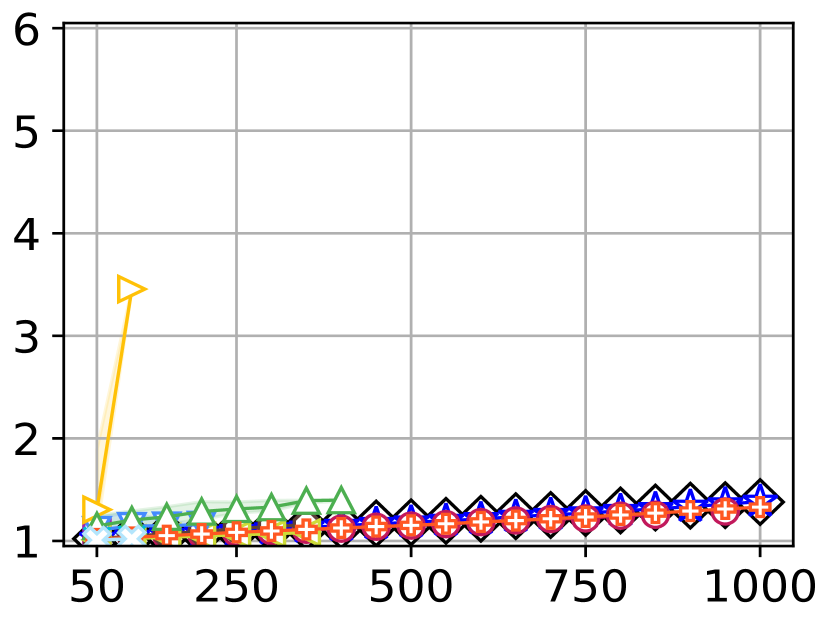
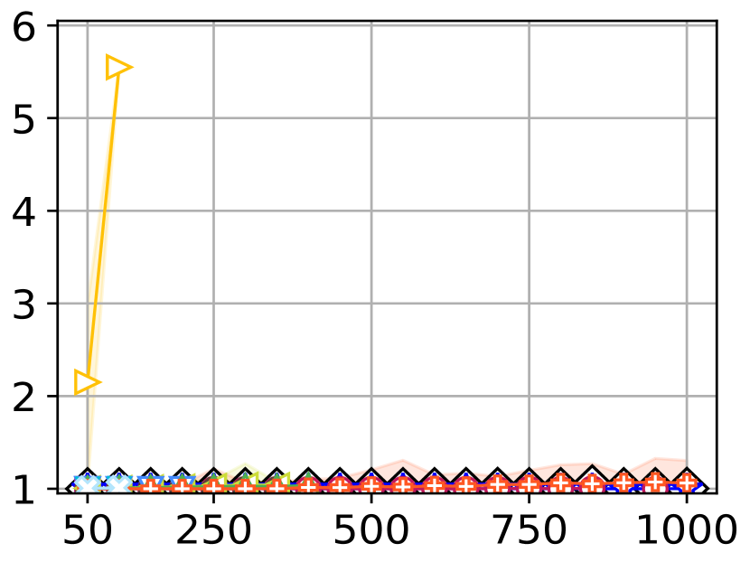
	lak303d 194x194 (14,784)	lt_gallowstemplar_n 251x180 (10,021)	maze-128-128-1 128x128 (8,191)	maze-128-128-10 128x128 (14,818)	maze-128-128-2 128x128 (10,858)	maze-32-32-2 32x32 (666)
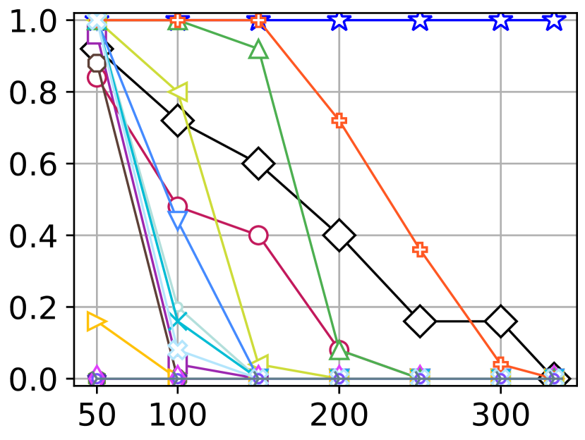
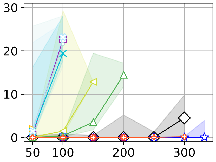
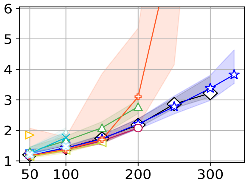
agents: $|A|$
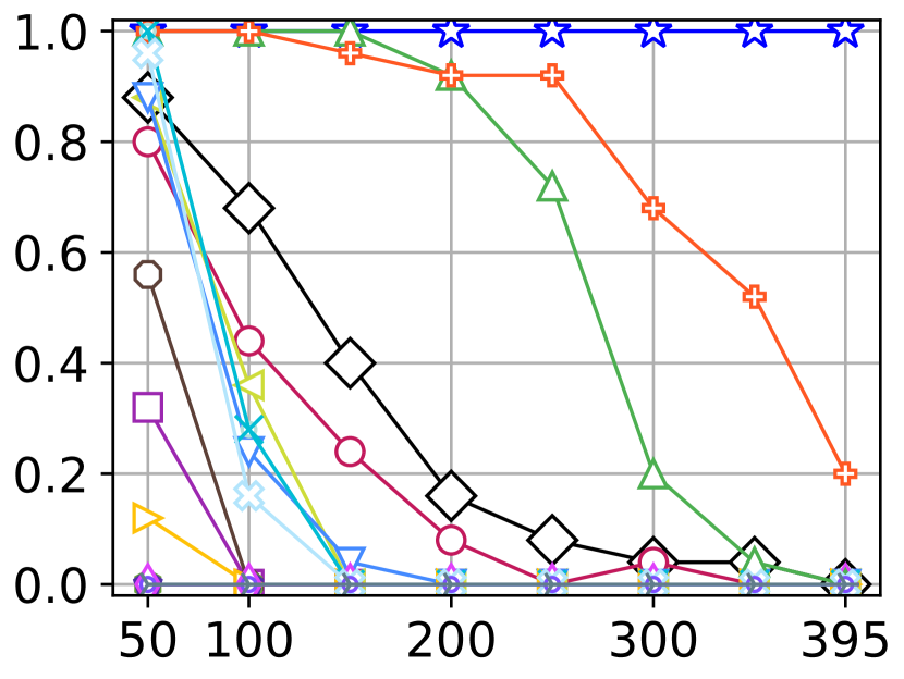
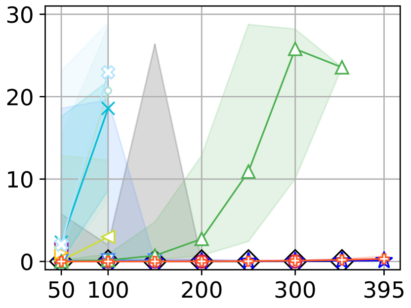
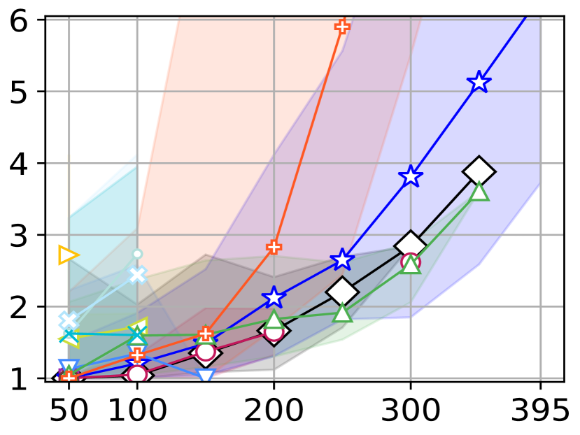
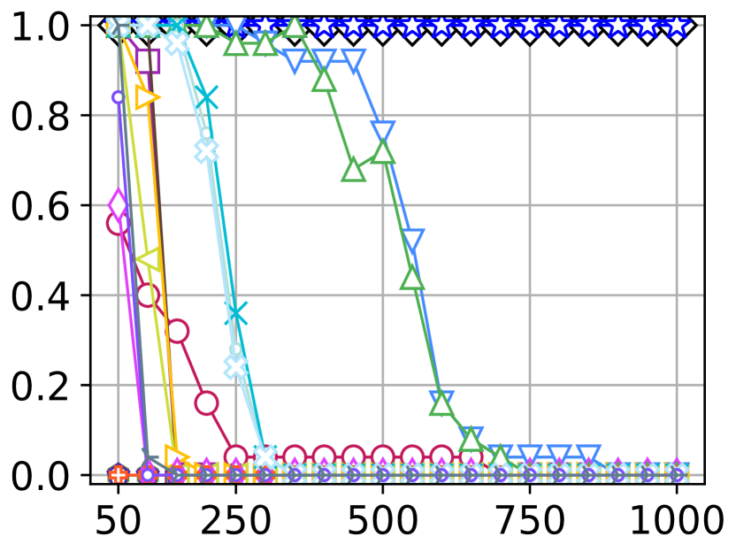
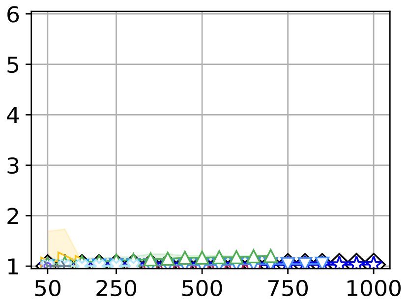
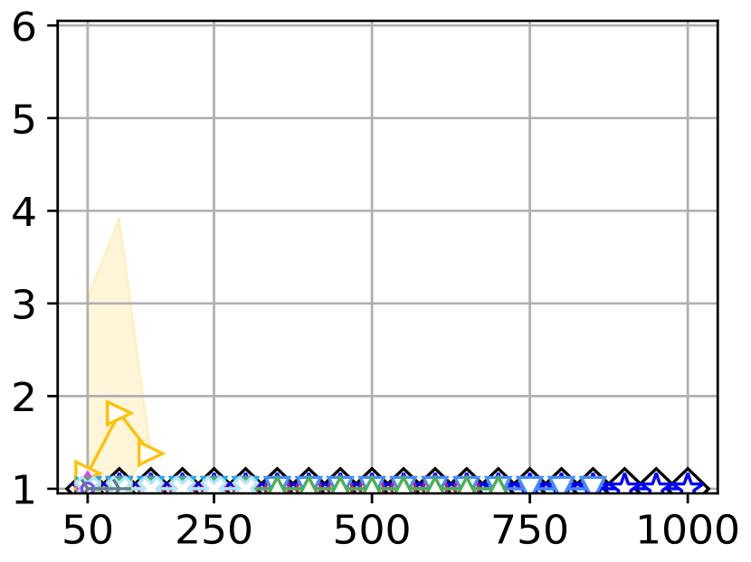
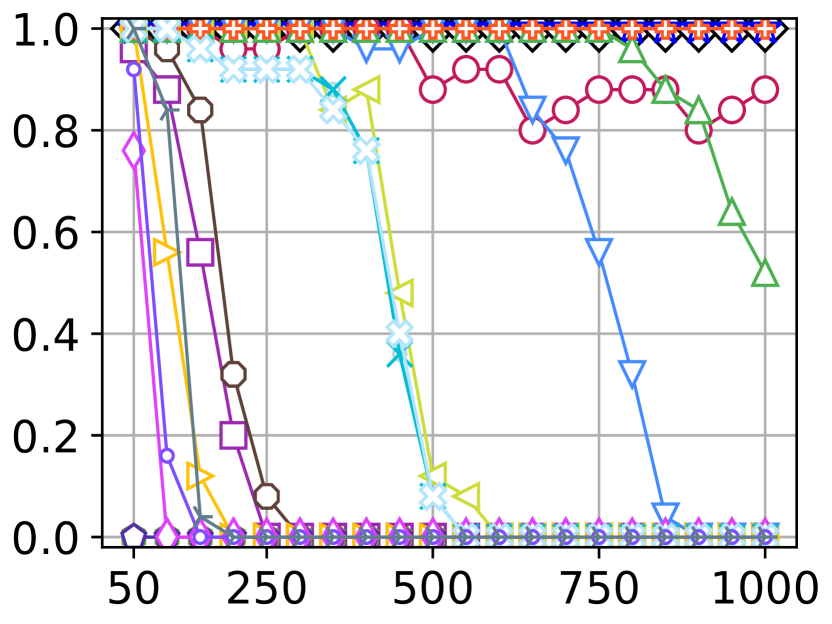
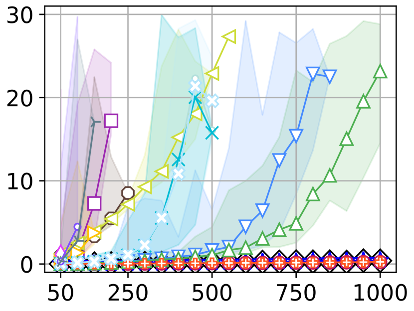
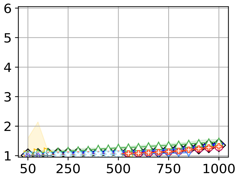
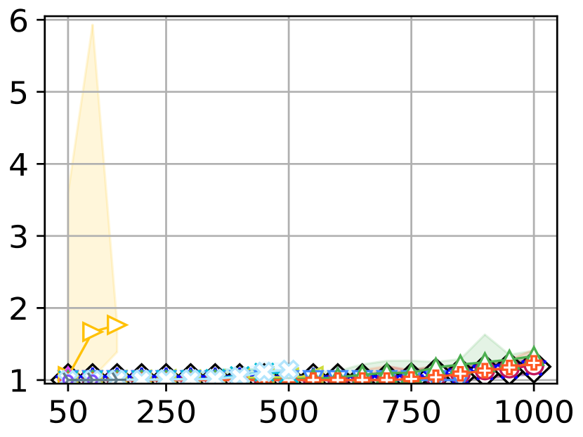
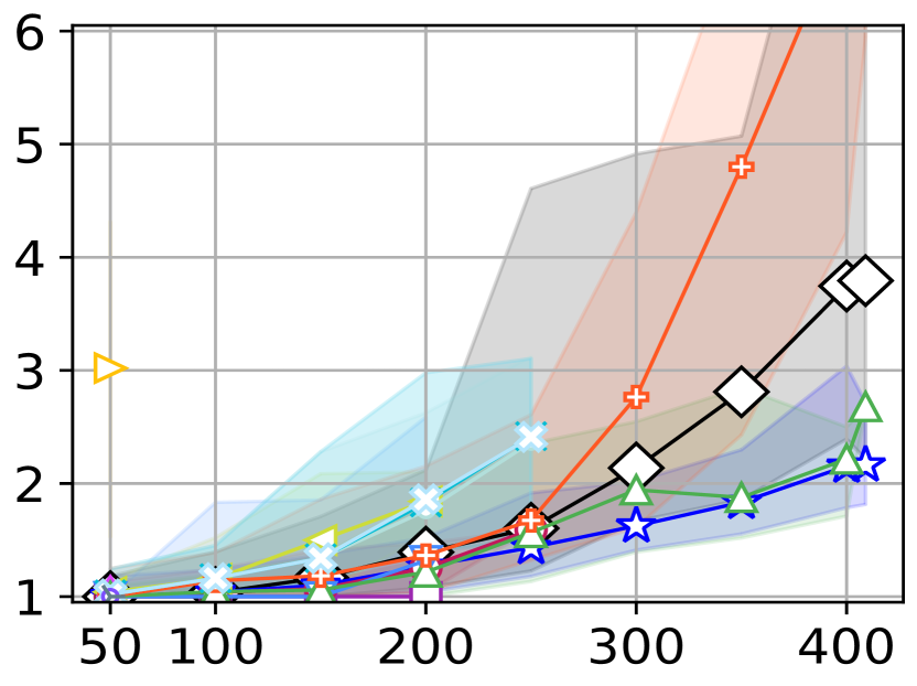
	maze-32-32-4 32x32 (790)	orz900d 1491x656 (96,603)	ost003d 194x194 (13,214)	random-32-32-10 32x32 (922)	random-32-32-20 32x32 (819)	random-64-64-10 64x64 (64x64)
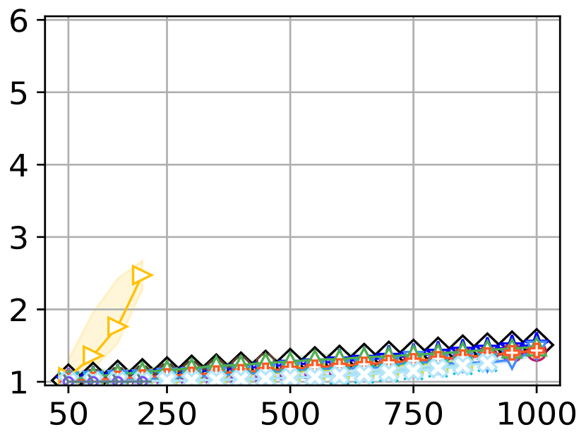
agents: $|A|$

Figure 11: Result of the MAPF benchmark (2/3). See also the caption of Fig. 8.

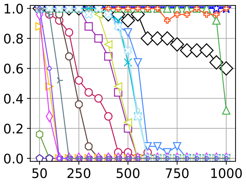
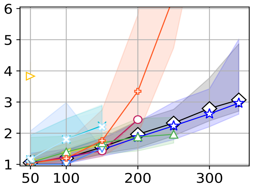
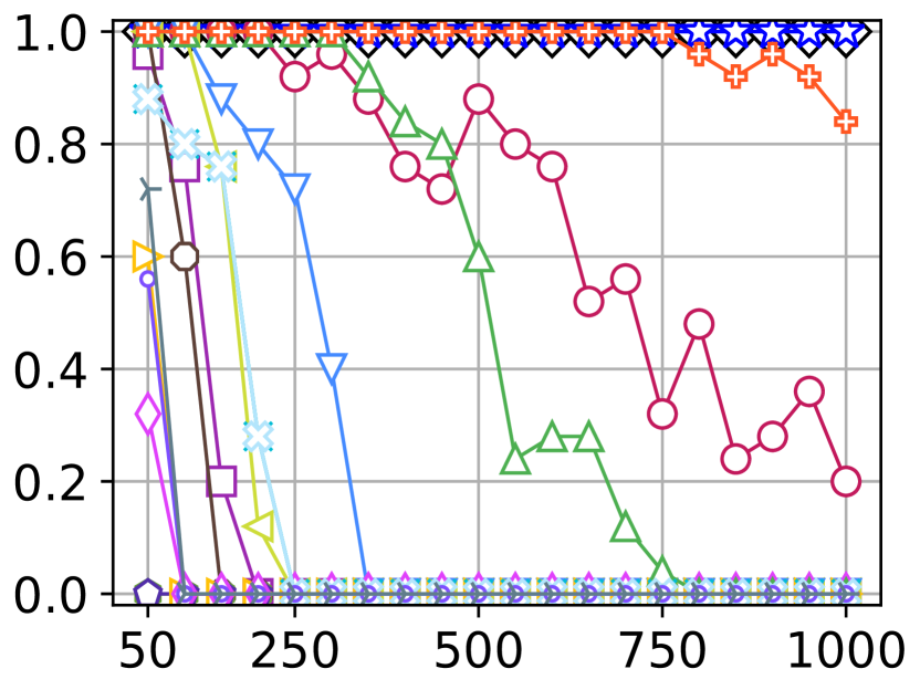
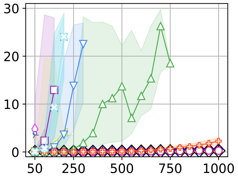
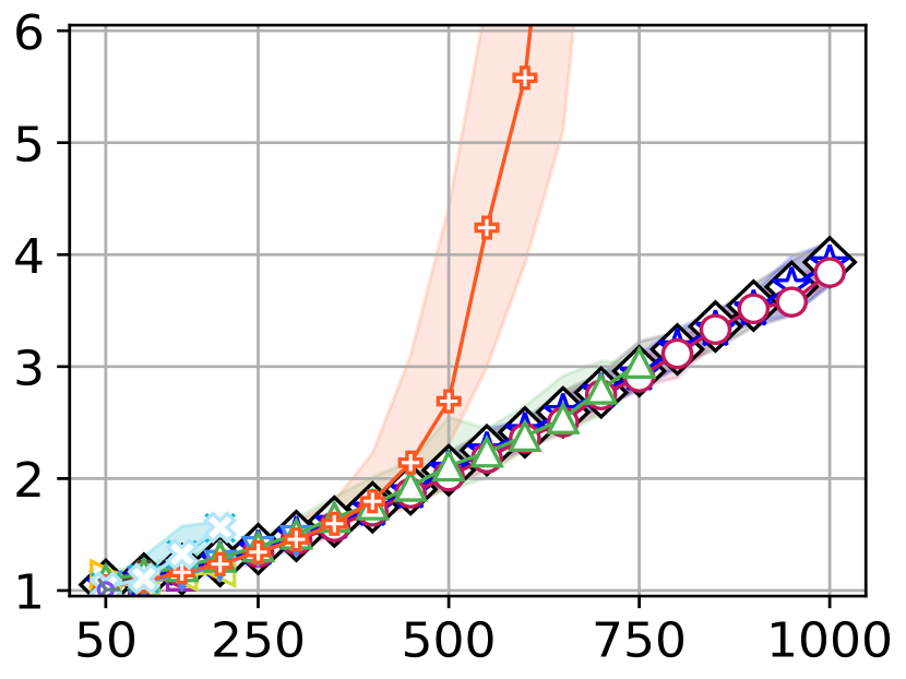
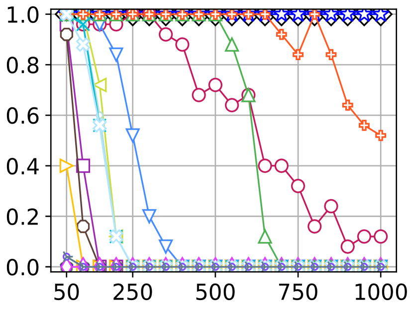
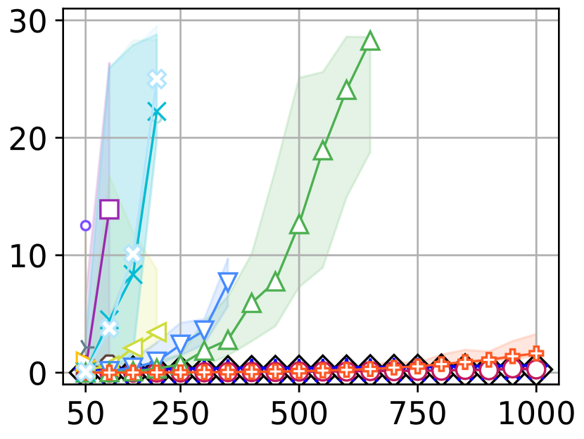
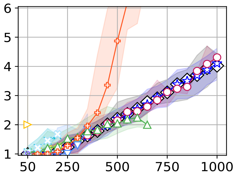
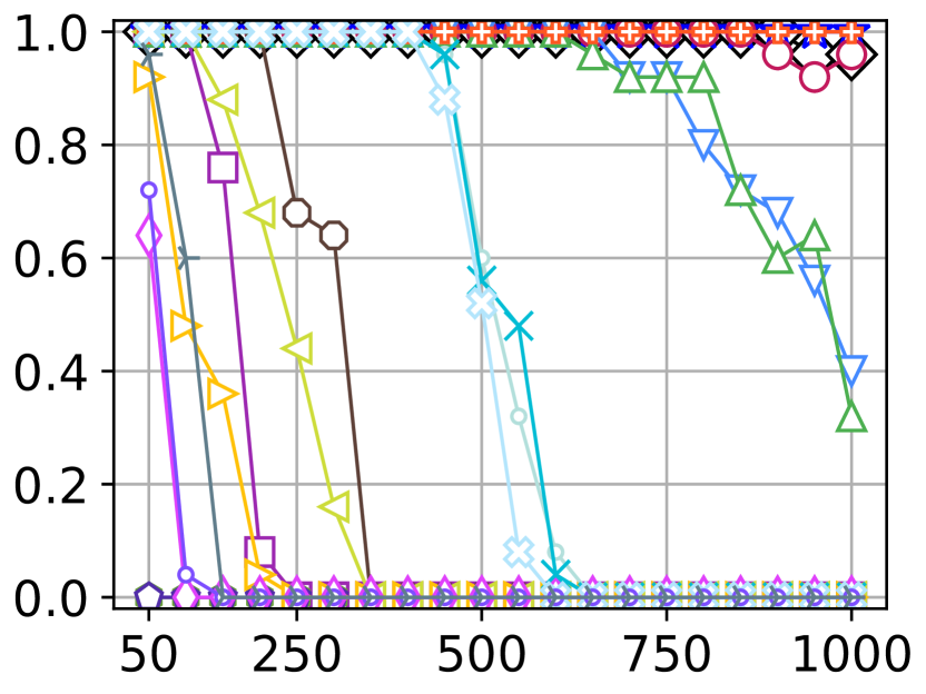
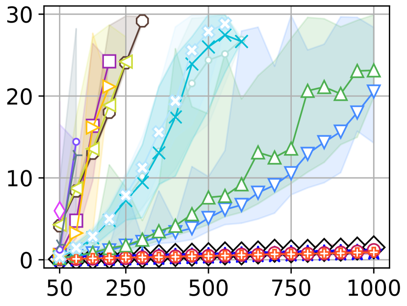
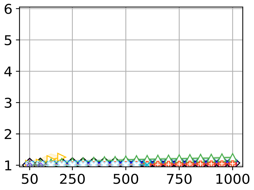
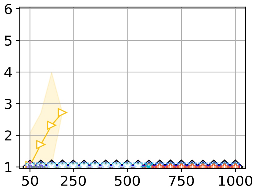
	random-64-64-20 64x64 (3,270)	room-32-32-4 32x32 (682)	room-64-64-16 64x64 (3,646)	room-64-64-8 64x64 (3,232)	w_woundedcoast 642x578 (34,020)	warehouse-10-20-10-2-1 161x63 (5,699)
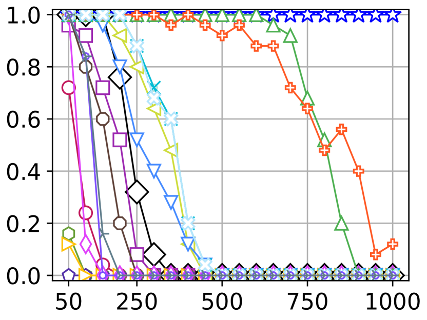
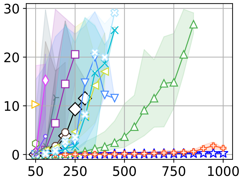
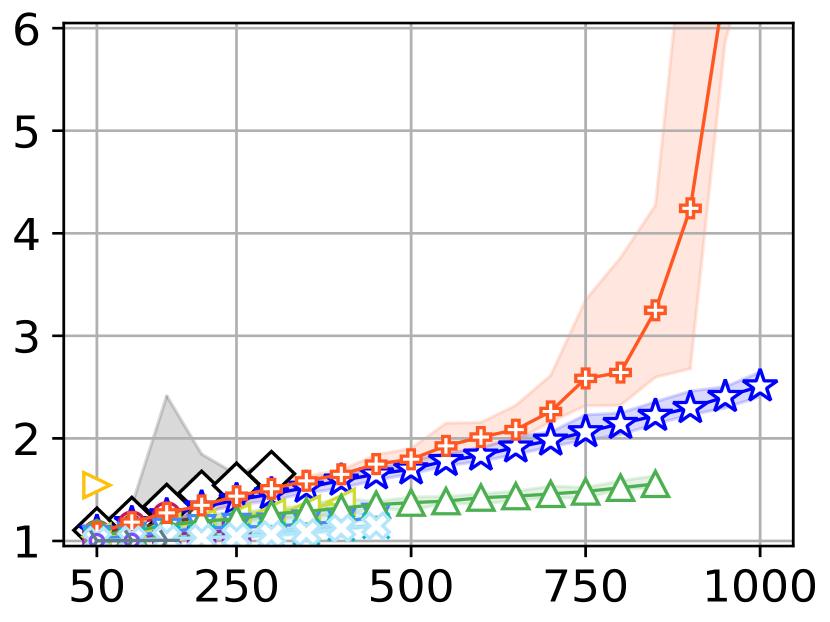
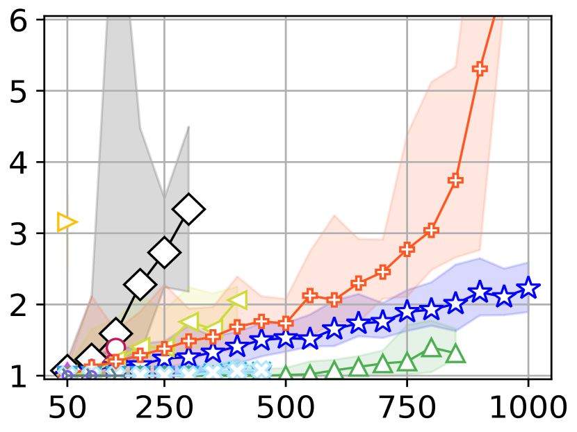
agents: $|A|$
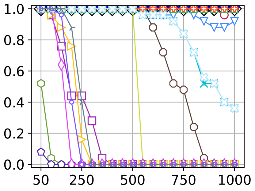
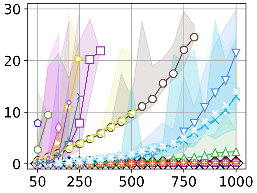
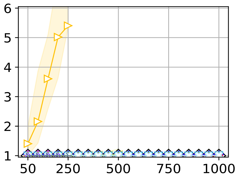
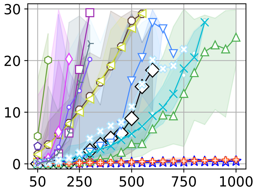
	warehouse-10-20-10-2-2 170x84 (9,776)	warehouse-20-40-10-2-1 321x123 (22,599)	warehouse-20-40-10-2-2 340x164 (38,756)
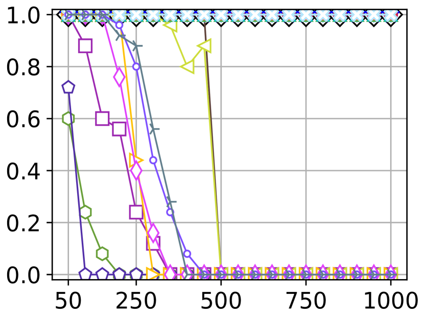
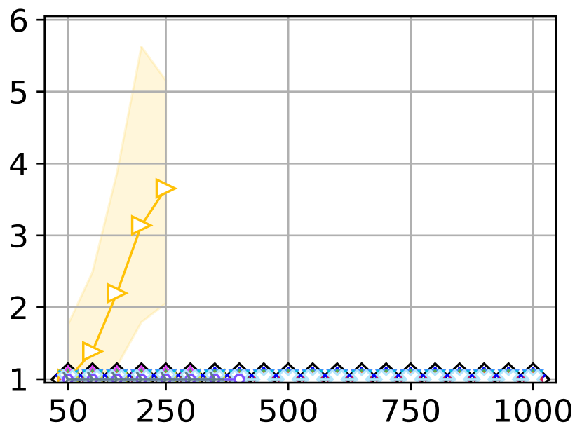
agents: $|A|$

Figure 12: Result of the MAPF benchmark (3/3). See also the caption of Fig. 8.

References

- Andreychuk and Yakovlev [2018] Anton Andreychuk and Konstantin Yakovlev. Two techniques that enhance the performance of multi-robot prioritized path planning. In Proc. Int. Joint Conf. on Autonomous Agents & Multiagent Systems (AAMAS), 2018.
- Cohen et al. [2018a] Liron Cohen, Matias Greco, Hang Ma, Carlos Hernández, Ariel Felner, TK Satish Kumar, and Sven Koenig. Anytime focal search with applications. In Proc Int. Joint Conf. on Artificial Intelligence (IJCAI), 2018.
- Cohen et al. [2018b] Liron Cohen, Glenn Wagner, David Chan, Howie Choset, Nathan Sturtevant, Sven Koenig, and TK Satish Kumar. Rapid randomized restarts for multi-agent path finding solvers. In Proc. Annu. Symp. on Combinatorial Search (SOCS), 2018.
- De Wilde et al. [2014] Boris De Wilde, Adriaan W Ter Mors, and Cees Witteveen. Push and rotate: a complete multi-agent pathfinding algorithm. Journal of Artificial Intelligence Research (JAIR), 2014.
- Erdmann and Lozano-Perez [1987] Michael Erdmann and Tomas Lozano-Perez. On multiple moving objects. Algorithmica, 1987.
- Goldenberg et al. [2014] Meir Goldenberg, Ariel Felner, Roni Stern, Guni Sharon, Nathan Sturtevant, Robert Holte, and Jonathan Schaeffer. Enhanced partial expansion A*. Journal of Artificial Intelligence Research (JAIR), 2014.
- Hart et al. [1968] Peter E Hart, Nils J Nilsson, and Bertram Raphael. A formal basis for the heuristic determination of minimum cost paths. IEEE transactions on Systems Science and Cybernetics, 1968.
- Karaman and Frazzoli [2011] Sertac Karaman and Emilio Frazzoli. Sampling-based algorithms for optimal motion planning. International Journal of Robotics Research (IJRR), 2011.
- Kautz et al. [2002] Henry Kautz, Eric Horvitz, Yongshao Ruan, Carla Gomes, and Bart Selman. Dynamic restart policies. In Proc. AAAI Conf. on Artificial Intelligence (AAAI), 2002.
- Lam et al. [2022] Edward Lam, Pierre Le Bodic, Daniel Harabor, and Peter J Stuckey. Branch-and-cut-and-price for multi-agent path finding. Computers & Operations Research (COR), 2022.
- Li et al. [2021a] Jiaoyang Li, Zhe Chen, Daniel Harabor, P Stuckey, and Sven Koenig. Anytime multi-agent path finding via large neighborhood search. In Proc Int. Joint Conf. on Artificial Intelligence (IJCAI), 2021.
- Li et al. [2021b] Jiaoyang Li, Daniel Harabor, Peter J Stuckey, and Sven Koenig. Pairwise symmetry reasoning for multi-agent path finding search. Artificial Intelligence (AIJ), 2021.
- Li et al. [2021c] Jiaoyang Li, Wheeler Ruml, and Sven Koenig. Eecbs: A bounded-suboptimal search for multi-agent path finding. In Proc. AAAI Conf. on Artificial Intelligence (AAAI), 2021.
- Li et al. [2022] Jiaoyang Li, Zhe Chen, Daniel Harabor, Peter J Stuckey, and Sven Koenig. Mapf-lns2: Fast repairing for multi-agent path finding via large neighborhood search. In Proc. AAAI Conf. on Artificial Intelligence (AAAI), 2022.
- Luna and Bekris [2011] Ryan Luna and Kostas E Bekris. Push and swap: Fast cooperative path-finding with completeness guarantees. In Proc Int. Joint Conf. on Artificial Intelligence (IJCAI), 2011.
- Okumura and Défago [2023] Keisuke Okumura and Xavier Défago. Quick multi-robot motion planning by combining sampling and search. In Proc Int. Joint Conf. on Artificial Intelligence (IJCAI), 2023.
- Okumura et al. [2021] Keisuke Okumura, Yasumasa Tamura, and Xavier Défago. Iterative refinement for real-time multi-robot path planning. In Proc. IEEE/RSJ Int. Conf. on Intelligent Robots and Systems (IROS), 2021.
- Okumura et al. [2022] Keisuke Okumura, Manao Machida, Xavier Défago, and Yasumasa Tamura. Priority inheritance with backtracking for iterative multi-agent path finding. Artificial Intelligence (AIJ), 2022.
- Okumura [2023] Keisuke Okumura. Lacam: Search-based algorithm for quick multi-agent pathfinding. In Proc. AAAI Conf. on Artificial Intelligence (AAAI), 2023.
- Sharon et al. [2015] Guni Sharon, Roni Stern, Ariel Felner, and Nathan R Sturtevant. Conflict-based search for optimal multi-agent pathfinding. Artificial Intelligence (AIJ), 2015.
- Shome et al. [2020] Rahul Shome, Kiril Solovey, Andrew Dobson, Dan Halperin, and Kostas E Bekris. drrt*: Scalable and informed asymptotically-optimal multi-robot motion planning. Autonomous Robots (AURO), 2020.
- Silver [2005] David Silver. Cooperative pathfinding. In Proc. AAAI Conf. on Artificial Intelligence and Interactive Digital Entertainment (AIIDE), 2005.
- Standley and Korf [2011] Trevor Standley and Richard Korf. Complete algorithms for cooperative pathfinding problems. In Proc Int. Joint Conf. on Artificial Intelligence (IJCAI), 2011.
- Standley [2010] Trevor Scott Standley. Finding optimal solutions to cooperative pathfinding problems. In Proc. AAAI Conf. on Artificial Intelligence (AAAI), 2010.
- Stern et al. [2019] Roni Stern, Nathan Sturtevant, Ariel Felner, Sven Koenig, Hang Ma, Thayne Walker, Jiaoyang Li, Dor Atzmon, Liron Cohen, TK Kumar, et al. Multi-agent pathfinding: Definitions, variants, and benchmarks. In Proc. Annu. Symp. on Combinatorial Search (SOCS), 2019.
- Surynek [2013] Pavel Surynek. Redundancy elimination in highly parallel solutions of motion coordination problems. International Journal on Artificial Intelligence Tools (IJAIT), 2013.
- Van Den Berg and Overmars [2005] Jur P Van Den Berg and Mark H Overmars. Prioritized motion planning for multiple robots. In Proc. IEEE/RSJ Int. Conf. on Intelligent Robots and Systems (IROS), 2005.
- Vedder and Biswas [2021] Kyle Vedder and Joydeep Biswas. X*: Anytime multi-agent path finding for sparse domains using window-based iterative repairs. Artificial Intelligence (AIJ), 2021.
- Wagner and Choset [2015] Glenn Wagner and Howie Choset. Subdimensional expansion for multirobot path planning. Artificial Intelligence (AIJ), 2015.
- Wurman et al. [2008] Peter R Wurman, Raffaello D’Andrea, and Mick Mountz. Coordinating hundreds of cooperative, autonomous vehicles in warehouses. AI magazine, 2008.
- Yu and LaValle [2013] Jingjin Yu and Steven M LaValle. Structure and intractability of optimal multi-robot path planning on graphs. In Proc. AAAI Conf. on Artificial Intelligence (AAAI), 2013.