Supervised Training of Neural-Network Quantum States for the Next-Nearest Neighbor Ising model

Abstract

Neural networks can be used to represent quantum states. Here we explore and compare different strategies for supervised learning of multilayer perceptrons. In particular, we consider two different loss functions which we refer to as mean-squared error and overlap, and we test their performance for the wave function in different phases of matter. For this, we consider the next-nearest neighbor Ising model because its ground state can be in various different phases. Of these phases, we focus on the paramagnetic, ferromagnetic, and pair-antiferromagnetic phases, while for the training we study the role of batch size, number of samples, and size of the neural network. We observe that the overlap loss function allows us to train the model better across all phases, provided one rescales the neural network.

I Introduction

The impact of machine learning models in the study of quantum physics is growing substantially [1, 2, 3, 4, 5]. Applications include use of neural networks for phase characterization [6, 7, 8], experimental guidance [9], state tomography [10, 11, 12, 13, 14, 15], process tomography [16, 17], control [18, 19, 20], learn Hamiltonians [21, 22, 23, 24, 25] and dissipators [26, 27], and to describe wave functions both for equilibrium and non-equilibrium cases, with supervised and unsupervised learning [28, 29, 30, 31, 32, 33, 34, 35, 36, 37, 38, 39, 40, 41, 42]. Regarding the description of a wave function, a current paradigm is that of the so-called neural-network quantum states (NNQS) in which the machine learning model, in physical terms the “ansatz”, takes as input a configuration of the quantum system, and returns the probability amplitude of the wave function. To ensure that the machine learning model parameters are optimized to describe the wave function, one can use either unsupervised or supervised learning. In an unsupervised search for the ground state, one optimizes the model parameters to decrease the total energy of the system [28]. For time evolution, one can estimate the equations of motion of the model parameters and integrate them [28, 33, 34]. Unsupervised optimization is frequently performed using stochastic reconfiguration [43], and it can be accelerated using transfer learning [39, 40], sequential local optimization [44] or computing the geometric tensor on the fly [45]. In supervised learning instead, one already has access to information about the probability amplitude of a (large) number of configurations and he/she can use this information to optimize the model parameters [7]. The training data can, for instance, come from other numerical simulations or, more importantly, from experiments. Supervised learning has two clear applications: (i) it can teach us whether a particular machine learning model is expressive enough and can be trained to represent a certain wave function. This information can be used to then select that model to describe similar systems, and/or to classify the types of physical systems and correlations that the machine learning model can describe. (ii) the representation of the wave function via the machine learning model can allow us to gather insights on the physical system which may be difficult to obtain from an experimental setup. For instance, not all observables (like long range correlations) or measurables (like entropy or out-of-time-ordered correlators [46]) are readily accessible on experimental platforms. One would thus train a neural network which represents the wave function of the system, and then interrogate the neural network to obtain the desired information about the state.

In this work, we study supervised learning using a multilayer perceptron (MLP) model applied to a physical system that has ferromagnetic, paramagnetic, antiferromagnetic and pair-antiferromagnetic phases (see discussion in Sec. III). We study the effectiveness and efficiency of training the MLP model as a function of the different phases, and of different model and learning parameters such as number of hidden nodes, loss function, number of training data, size of the batches of training data, and learning rates. Across the different phases examined, we show that the mean squared error (MSE) loss function generally produces less accurate wave functions than another loss function which we will refer to as “overlap loss function”, provided that, for the latter, we rescale the output of the neural network. We also see that sample sizes should be particularly large, especially when studying paramagnetic phases and using small batch sizes for the training samples is typically an effective regularization parameter.

The paper is structured in the following manner: In Sec. II we describe NNQS, the supervised training, and the two loss functions considered; In Sec. III we describe the physical system studied and its properties; In Sec. IV we present our results and their analysis and in Sec. V we draw our conclusions.

II Supervised Neural-Network Quantum States

Figure 1: Multilayer perceptron architecture. Inputs are $x_{m,i}$, the elements of a spin configuration ${\bm{x}_{m}}$, $L$ is the number of spins of the system, with one hidden layer of $\alpha L$ and output the $\ln(\Psi({\bm{x}_{m}}))$.

Neural-network quantum states belong to the family of variational Monte Carlo methods that use neural networks as the trial wave function. They were proposed by the authors of [28] with the aim to represent the amplitudes of a quantum state $\Psi(\bm{x_{m}})$ for a certain configuration $\bm{x_{m}}$ with a neural network. Here, our choice of the neural network is a multilayer perceptron, where each visible node represents one of the $L$ particles of the quantum many-body system. More specifically, here a visible node can take the values $-1$ or $1$ depending on whether the spin at that location is pointing down or up respectively. Fig. 1 shows a depiction of a multilayer perceptron with a single hidden layer. Note that the output layer returns the logarithm of the probability amplitude associated with one configuration, i.e. $\ln(\Psi({\bm{x}_{m}}))$, because the wave function typically takes values that vary over different orders of magnitude. One advantage of a multilayer perceptron is its flexible design and deeper structure, compared to restricted Boltzmann machines.

In the multilayer perceptron neural-network quantum state, we use a concatenation of linear and nonlinear functions given by

$$\ln\left[\Psi(\bm{x_{m}})\right]=\sigma^{(k)}(\bm{W}^{(k)}\dots\sigma^{(1)}(\bm{W}^{(1)}\bm{x_{m}}+\bm{b}^{(1)})\dots+\bm{b}^{(l)})$$ (1)

where $\bm{W}^{(k)}\bm{x_{m}}+\bm{b}^{(k)}$ is the linear part at layer $k$, while $\sigma^{(k)}$ is the nonlinear activation function at layer $k$. In our case, it is sufficient to consider a single hidden layer. The number of nodes in this layer is given by $\alpha L$ where we refer to $\alpha$ as the hidden ratio. For the activation function $\sigma^{(k)}$, for $k=1$ we use leaky ReLU [47], which is given by

$$\text{LeakyReLU}(x)=\begin{cases}x&\text{if }x\geq 0\\ \gamma x&\text{otherwise}\end{cases}$$

Where $\gamma$ is a constant we choose to fix it as 0.01 for our experiments. The use of this activation function can prevent saturation gradient, which could happen with ReLU.

The supervised training of neural-network quantum states is completely analogous to the regression problem in common machine learning settings. We used labeled data $(\bm{x_{m}},\ln[\Psi_{G}(\bm{x_{m}}))]$ pairs, where $\Psi_{G}(\bm{x_{m}})$ is the exact value of probability amplitude for the spin configuration $\bm{x_{m}}$. Here $m$ goes from $1$ to $M$, while $M_{u}$ is the number of unique samples, as sometimes many could be repeated. The samples should be representative of the probability distribution stemming from the wave function, and they could come from experimental data, although here we use numerically generated ones. In the following, we also use the notation $\ln(\tilde{\Psi}({\bm{x}}_{m}))$ for the rescaled output of the neural network, which is given by

$$\ln(\tilde{\Psi}({\bm{x}}_{m}))=\frac{\ln(\Psi({\bm{x}}_{m}))}{\max_{k}\ln(\Psi({\bm{x}}_{k}))}$$ (2)

which is the output of the neural network divided by the maximum occurring for the configurations considered. It follows that $\tilde{\Psi}({\bm{x}}_{m})=\exp[\ln(\tilde{\Psi}({\bm{x}}_{m}))]$.

To obtain $\Psi_{G}(\bm{x_{m}})$, we use a matrix product states algorithm with the zipper method to obtain the samples [48, 49]. While the total size of the possible labeled data is $2^{L}$, where $L$ is the size of the system under study, in general, we can only take a much smaller number of sample $M$ drawn from the distribution $|\Psi_{G}(\bm{x_{m}})|^{2}$ using the Metropolis-Hastings algorithm [50, 51].

To train the neural-network quantum state in a supervised manner, we need a loss function to be minimized. Between the variety of possible loss functions, we here consider the mean squared error (MSE)

$$\mathcal{L}_{\text{MSE}}(\Psi_{G},\Psi)=\frac{1}{M}\sum_{m}^{M}\Big{(}\ln{\Psi_{G}(\bm{x_{m}})}-\ln{\Psi(\bm{x_{m}})}\Big{)}^{2}$$ (3)

and the overlap

$$\begin{split}\mathcal{L}_{\text{Overlap}}(\tilde{\Psi}_{G},\tilde{\Psi})&=-\ln\left[\frac{\braket{\tilde{\Psi}_{G}\mid\tilde{\Psi}}\braket{\tilde{\Psi}\mid\tilde{\Psi}_{G}}}{\braket{\tilde{\Psi}_{G}\mid\tilde{\Psi}_{G}}\braket{\tilde{\Psi}\mid\tilde{\Psi}}}\right],\end{split}$$ (4)

where

$$\braket{\tilde{\Psi}_{A}\mid\tilde{\Psi}_{B}}=\sum_{m}^{M_{u}}\tilde{\Psi}_{A}^{*}(\bm{x_{m}})\tilde{\Psi}_{B}(\bm{x_{m}}),$$ (5)

also used in [52]. Here we used $\tilde{\Psi}_{\beta}(\bm{x_{m}})$, where $\beta=A,B\dots$, and not $\Psi_{\beta}(\bm{x_{m}})$, because we need to exponentiate the output of the neural network and this can lead to instabilities, see [45] and App. A. We note that in Eq. (4-5) we use the unique samples $M_{u}$ instead of all the samples. This is because otherwise the normalization will be skewed towards the more probable configurations [53] . We then compute the gradient of the loss functions and update the parameters using an initial learning rate $\gamma$ and Adam optimizer introduced in  [54, 55].

III The Next-nearest Neighbor Ising model

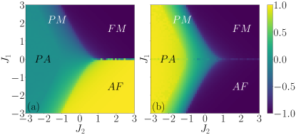
Figure 2: Phase diagram of the next-nearest neighbor Ising model, Eq. (6), in terms of tunneling $J_{1}$ and $J_{2}$ interactions. (a) Nearest-neighbor correlation $C_{NN}$ from Eq. (7); (b) Next-nearest neighbor correlation $C_{NNN}$ from Eq. (8). Parameters $h_{x}=1$, system size $L=128$. Paramagnetic region is labeled by $PM$, ferromagnetic by $PM$, antiferromagnetic by $AF$ and pair-antiferromagnetic by $PA$.

While supervised training can, in principle, be used to learn any type of state we here focus on training ground states with different properties. The main reason is that with the methods we use to generate data, i.e. matrix product states, ground states can be efficiently and effectively produced [56]. Hence, for our analysis, we choose the next-nearest neighbor Ising model whose ground state can be in four different phases. More specifically, the Hamiltonian is given by

$$H=-h_{x}\sum_{l=1}^{L}\sigma^{x}_{l}-J_{1}\sum_{l=1}^{L}\sigma^{z}_{l}\sigma^{z}_{l+1}-J_{2}\sum_{l=1}^{L}\sigma^{z}_{l}\sigma^{z}_{l+2}$$ (6)

where $\sigma^{a}_{l}$ are the corresponding Pauli matrices (with $a=x,y,z$) at site $l$. $h_{x}$ is the magnetic field along the $x$ axis, and $J_{1}$ and $J_{2}$ are, respectively, nearest neighbor and next-nearest neighbor couplings. We note that the Hamiltonian has a “particle-hole” symmetry such that one can map an Hamiltonian with coupling $J_{1}$ to one with coupling $-J_{1}$ via the operator $S=\prod_{j}\sigma^{x}_{2j}$, i.e. $H(J_{1})=SH(-J_{1})S^{\dagger}$. This transformation, for instance, turns a ferromagnetic phase into an antiferromagnetic phase, and it is thus sufficient to study the system for positive values of $J_{1}$. The phase diagram, described in terms of $J_{1}$ and $J_{2}$, is depicted in Fig. 2 for $h_{x}=1$ which is the energy scale that we use throughout the paper. To compute the ground state we have used a matrix product states code built using ITensor libraries  [57]. To identify the phases we use the nearest-neighbor ferromagnetic correlator $C_{NN}$ given by

$$C_{NN}=-\dfrac{1}{L-1}\sum_{l=1}^{L-1}\sigma^{z}_{l}\sigma^{z}_{l+1}$$ (7)

depicted in Fig. 2(a), and the next-nearest neighbor antiferromagnetic correlator $C_{NNN}$ given by

$$C_{NNN}=\dfrac{1}{L-2}\sum_{l=1}^{L-2}\sigma^{z}_{l}\sigma^{z}_{l+2}$$ (8)

shown in Fig. 2(b). In the ferromagnetic phase $C_{NN}$ and $C_{NNN}$ are both large and negative. In the pair-antiferromagnetic phase, e.g. spin configurations of the type $\uparrow\uparrow\downarrow\downarrow\uparrow\uparrow\downarrow\downarrow$, only $C_{NNN}$ is large and positive while $C_{NN}$ approaches zero. Between these two phases, one encounters the paramagnetic phase, for which both order parameters are small. For negative $J_{1}$, we can obtain the possible phases by applying the operator $S$ and thus results in an antiferromagnetic phase and another pair-antiferromagnetic phase, separated by a paramagnetic phase. We also note that for $J_{1}>0$, the probability amplitude $\Psi({\bm{x}_{m}})$ can be written as a positive real number, and thus one can use a multilayer perceptron model with real weights and biases, without the need for complex numbers.

IV Results

In the following, we study the performance of training the multilayer perceptron with different loss functions and other training parameters for the system being in different phases of matter. We consider a large system with $L=128$. One important training parameter we consider is the number of training samples $M$, which if not stated otherwise we consider to be $10^{5}$. For $\mathcal{L}_{\rm Overlap}$, we first obtain the $M$ samples, then only use the corresponding $M_{u}$ unique ones to update the neural network. During the training, we typically only use a portion of these data to evaluate the loss function and optimize the parameters at each epoch. This portion of the data is called batch size and we refer to it with the symbol $B$. Another parameter we vary is the hidden ratio $\alpha$, which if not stated otherwise, we set to $\alpha=3$.

To evaluate how well our training works, we study the relative energy error $\mathcal{E}_{r}$ given by

$$\mathcal{E}_{r}=\left|\frac{E_{T}-E_{G}}{E_{G}}\right|,$$ (9)

where $E_{G}$ is the ground state energy computed from matrix product states computations, while $E_{T}$ is the energy of the trained wave function. For the trained wave function, we evaluate the energy by

$$E_{T}=\sum_{m=1}^{M}\frac{1}{M}E_{\rm loc}({\bm{x}_{m}}),$$ (10)

when using $\mathcal{L}_{\rm MSE}$, as we use all the $M$ samples, and

$$E_{T}=\sum_{m=1}^{M_{u}}|\Psi(\bm{x}_{m})|^{2}E_{\rm loc}({\bm{x}_{m}}),$$ (11)

when using $\mathcal{L}_{\rm Overlap}$ because it used only the unique samples $M_{u}$. In Eqs.(10, 11), the local energy $E_{\rm loc}$ is given by

$$E_{\rm loc}({\bm{x}_{m}})=\sum_{m^{\prime}}H_{m^{\prime},m}\frac{\Psi({\bm{x}_{m^{\prime}}})}{\Psi({\bm{x}_{m}})}.$$ (12)

Here $H_{m^{\prime},m}$ is the matrix element of the Hamiltonian which connects the two configurations ${\bm{x}_{m}}$ and ${\bm{x}_{m^{\prime}}}$. Naturally, if we knew already what the Hamiltonian was, we could have done the unsupervised training, but here we use the Hamiltonian to have a quantitative idea of how close we are to the state we try to represent.

IV.1 Training in the paramagnetic phase

Results for the paramagnetic phase are shown in Fig. 3. Here, the parameters are $J_{1}=2$ and $J_{2}=-1$, and we have used an initial learning rate $\gamma=10^{-5}$. The default parameters, unless stated otherwise, are the number of samples $M=10^{5}$, batch size $B=32$, and hidden ratio $\alpha=3$. In Fig. 3(a,c,e) we show results for the loss function $\mathcal{L}_{\rm Overlap}$, while in panels (b,d,f) we have considered $\mathcal{L}_{\rm MSE}$. In panels (a) and (b) we keep all parameters the same except for the batch size $B$, in panels (c) and (d) we vary the number of samples, and in panels (e) and (f) we consider different hidden ratios $\alpha$.

In all panels, we look at the relative error of the energy $\mathcal{E}_{r}$ versus the number of epochs $E$. We observe that both loss functions allow reaching low relative errors of the order of $10^{-2}$ [58]. In general, both a smaller batch size, see App. B, and a larger number of samples result in better performance, although the performance will be slower. Furthermore, for both loss functions, a larger hidden ratio can result in better performance.

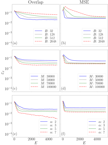
Figure 3: Relative error $\mathcal{E}_{r}$ for the paramagnetic ground state ($J_{1}=2$ and $J_{2}=-1$) versus number of epochs $E$. In panel (a, c, e) we use overlap loss function $\mathcal{L}_{\rm Overlap}$, while in panel (b, d, f) we use $\mathcal{L}_{\rm MSE}$. In panels (a,b) we vary the batch size, in panels (c,d) we vary the number of samples, and in panels (e,f) we vary the hidden ratio $\alpha$. If not stated otherwise, the number of training samples is $M=10^{5}$, the hidden ratio is $\alpha=3$, the batch size is $B=32$ and $\gamma=10^{-5}$ is the initial learning rate.

IV.2 Training in the ferromagnetic phase

We here consider the ferromagnetic phase, for parameters $J_{1}=1$ and $J_{2}=2$, initial learning rate $\gamma=10^{-5}$. The default values, unless otherwise stated, are $M=10^{5}$ for the number of samples, $\alpha=3$ for the hidden ratio, $B=32$ for the batch size, and $\gamma=10^{-5}$ for the initial learning rate. The results are shown in Fig. 4, in a similar structure as in Fig. 3.

In Fig. 4 we observe that in some cases the error becomes very small and then it increases. This is due to the fact that in those cases the energy starts from below the ground state value, then goes above it, and then may decrease again approaching the exact value from above. Overall, in the ferromagnetic phase, we observe a similar behavior as with the paramagnetic phase, although we are able to reach more accurate predictions of the energy, with an error of the order of $10^{-3}$ or even smaller. Smaller batch sizes are generally helpful for both loss functions, and so are more number of samples, while a larger number of hidden nodes seems to lead to overfitting for $\mathcal{L}_{\rm Overlap}$, Fig. 4(e), while it still allows (marginal) improvements for $\mathcal{L}_{\rm MSE}$, Fig. 4(f). In general, we still observe that $\mathcal{L}_{\rm Overlap}$ allows us to reach energies closer to the ground state energy.

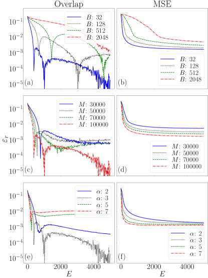
Figure 4: Relative error $\mathcal{E}_{r}$ for the ferromagnetic ground state ($J_{1}=1$ and $J_{2}=2$) versus number of epochs $E$. In panel (a, c, e) we use overlap loss function $\mathcal{L}_{\rm Overlap}$, while in panel (b, d, f) we use $\mathcal{L}_{\rm MSE}$. In panels (a,b) we vary the batch size, in panels (c,d) we vary the number of samples, and in panels (e,f) we vary the hidden ratio $\alpha$. If not stated otherwise, the number of training samples is $M=10^{5}$, the hidden ratio is $\alpha=3$, the batch size is $B=32$ and $\gamma=10^{-5}$ is the initial learning rate.

IV.3 Training in the pair-antiferromagnetic phase

In the pair-antiferromagnetic phase, the shown results are significantly affected by the fact that the initial energy of the state is below the ground state energy, and it requires a larger number of epochs to approach the ground state. Note that here we computed $10^{4}$ epochs as the model has slower optimization dynamics. In general, we still observe some form of overfitting for $\mathcal{L}_{\rm Overlap}$, Fig. 5(e), and a general improvement of performance with an increasing number of samples $M$, Fig. 5(c,d). As for the batch size, a smaller batch size optimizes in a smaller number of epochs as shown by an earlier crossing of the ground state energy, Fig. 5(a,b).

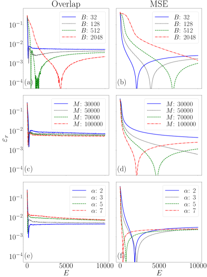
Figure 5: Relative error $\mathcal{E}_{r}$ for the pair-antiferromagnetic ground state ($J_{1}=1$ and $J_{2}=-2$) versus number of epochs $E$. In panel (a, c, e) we use overlap loss function $\mathcal{L}_{\rm Overlap}$, while in panel (b, d, f) we use $\mathcal{L}_{\rm MSE}$. In panels (a,b) we vary the batch size, in panels (c,d) we vary the number of samples, and in panels (e,f) we vary the hidden ratio $\alpha$. If not stated otherwise, the number of training samples is $M=10^{5}$, the hidden ratio is $\alpha=3$, the batch size is $B=32$ and $\gamma=10^{-5}$ is the initial learning rate.

IV.4 Convergence of loss function and relative energy error

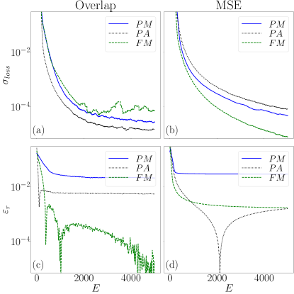
Figure 6: (a,b) Variance of the loss function value $\sigma_{loss}$ verus number of epochs $E$. (c,d) Relative energy error $\mathcal{E}_{r}$ versus the number of epochs $E$. Panels (a,c) are for $\mathcal{L}_{\rm Overlap}$, and panels (b,d) are for $\mathcal{L}_{\rm MSE}$. The blue continuous line is for the paramagnetic regime $J_{1}=2$ and $J_{2}=-1$, the grey dotted line for the pair-antiferromagnetic regime $J_{1}=1$ and $J_{2}=-2$, and the green dashed line for the ferromagnetic regime $J_{1}=1$ and $J_{2}=2$. In all panels we have used $B=32$, $M=10^{5}$, $\alpha=3$ and $\gamma=10^{-5}$.

In supervised training one typically only has access to data such as configurations and their corresponding probability amplitude, and not to the Hamiltonian of the system. During the training, we can monitor the evolution of the loss function, but this does not directly imply that other properties of the system, such as the energy, are better represented. We thus study the convergence of a loss function and compare that to the relative energy error $\mathcal{E}_{r}$. For the loss function, we evaluate the variance of the loss function $\sigma_{loss}$ over the past 200 epochs and we plot it against the epoch number. This is because a natural stopping criterion for the optimization is indeed that the variation of the loss function over the epochs is below a certain threshold.

In Fig. 6 we show this comparison between the standard deviation of the loss function $\sigma_{loss}$ over the past 200 epochs, panels (a,b), and the relative energy error $\mathcal{E}_{r}$ panels (c,d), both versus the number of epochs $E$. In panels (a,c) we consider the training with the loss function $\mathcal{L}_{\rm Overlap}$, while in panels (b,d) we used the loss function $\mathcal{L}_{\rm MSE}$. In each panel the blue continuous line corresponds to the paramagnetic regime ($J_{1}=2$ and $J_{2}=-1$), the grey dotted line to the pair-antiferromagnetic regime ($J_{1}=1$ and $J_{2}=-2$), and the green dashed line to the ferromagnetic regime ($J_{1}=1$ and $J_{2}=2$). We observe that, generally, a decrease in the loss function indeed results in a wave function with energy closer to the ground state energy, however, a quantitative correspondence between the two is not guaranteed.

V Conclusion

We have studied the supervised training of a neural network to represent the ground states of a Hamiltonian. We considered a Hamiltonian which presents various phases of matter, a paramagnetic phase, a ferromagnetic phase, and a pair-antiferromagnetic phase. For the training, we focused on two types of loss functions, one that tries to maximize the overlap between the trained data and the neural network wave function, $\mathcal{L}_{\rm Overlap}$, and one that tries to reduce the difference between the logarithm of the probability amplitudes and the output of the neural network $\mathcal{L}_{\rm MSE}$. We observed that in general the loss function $\mathcal{L}_{\rm Overlap}$ results in wave functions with better ground state energy in all phases considered. We note that it is important that for overlap the neural network output is rescaled to increase the stability of the algorithm, see App. A. Smaller batch sizes also tend to result in better performance, but this is also at the expense of computation time, see App. B. Furthermore, in general, larger sample sizes help obtain better results, but larger hidden dimensions can result, especially when using $\mathcal{L}_{\rm Overlap}$, in overfitting.

Future works could focus on the supervised learning for wave functions that cannot be described by real positive numbers, for example for a more complex ground state, an excited state (but still an eigenstate of the system), or even non-equilibrium states which behave like steady states [59, 60].

Appendix A Not rescaled wave function for overlap KL divergence loss functions

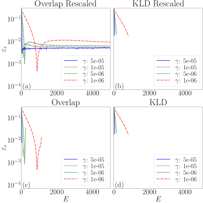
Figure A1: Relative error $\mathcal{E}_{r}$ for the pair-antiferromagnetic ground state ($J_{1}=1$ and $J_{2}=-2$) versus number of epochs $E$. (a) is the rescaled version of overlap. (b) is the rescaled version of KL divergence. (c) is the original overlap and (d) is the original KL divergence We vary to different learning rates compared to our control/default $10^{-5}$ in the paper. the number of training sample is $M=10^{5}$, batch size $B=32$, and the hidden ratio is $\alpha=3$.

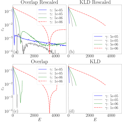
Figure A2: Relative error $\mathcal{E}_{r}$ for the ferromagnetic ground state ($J_{1}=1$ and $J_{2}=2$) versus number of epochs $E$. (a) is the rescaled version of overlap. (b) is the rescaled version of KL divergence. (c) is the original overlap and (d) is the original KL divergence We vary to different learning rates compared to our control/default $10^{-5}$ in the paper. the number of training sample is $M=10^{5}$, batch size $B=32$, and the hidden ratio is $\alpha=3$.

In the main portion of the article, we rescale the scalar product shown in Eq. (5). Here we show that if we were not to do this, the training would be more unstable and it could lead to the network parameters becoming ${\rm NaN}$. This is a general result, as we show by discussing two loss functions, the overlap loss function $\mathcal{L}_{\rm Overlap}$ and the Kullback–Leibler (KL) divergence. In this work, the loss function for KL divergence is given by

$$\mathcal{L}_{\rm KLD}(\Psi_{G},\Psi)=\sum_{m=1}^{M_{u}}{|\Psi_{G}({\bm{x}}_{m})|^{2}}\ln\left(\frac{|\Psi_{G}({\bm{x}}_{m})|^{2}}{|\Psi({\bm{x}}_{m})|^{2}}\right).$$ (13)

where the wave functions could be rescaled, i.e. each one is divided by the maximum value obtained over the $M_{u}$ unique samples, or not. Our results are shown in Fig. A1 and Fig. A2, respectively for parameters such that the ground state is in the pair-antiferromagnetic and in the ferromagnetic phase (the paramagnetic phase is more stable). In the figures, an interrupted line before 5000 epochs signifies that the training leads to ${\rm NaN}$ for the network parameters. Importantly, we note that even using a rescaled neural network for the KL divergence loss function can result in instability of the learning dynamics, as shown by the interruption of the lines.

In general, however, we note that using a smaller initial learning rate $\gamma$ results in a delayed instability of the neural network parameters’ dynamics.

Appendix B Smaller batch size for training

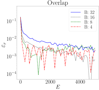
Figure A3: Relative error $\mathcal{E}_{r}$ for the paramagnetic ground state ($J_{1}=2$ and $J_{2}=-1$) versus number of epochs $E$. we use overlap loss function $\mathcal{L}_{\rm Overlap}$ and vary to smaller batch size compared to our control/default 32 in the paper. The number of the training samples is $M=10^{5}$, the learning rate is $10^{-4}$ and the hidden ratio is $\alpha=3$.

In the main portion of the article, we have observed that the smaller the batch size the better the wave function approaches the ground state energy. Here we explore this further with even smaller batch sizes using $\mathcal{L}_{\rm Overlap}$ as a loss function. In Fig. A3 we show results for 128 spins in the paramagnetic phase versus the number of epochs. We observe that smaller batch sizes can result in larger oscillations and not significant improvements while, not shown, requiring more time. For these reasons, we kept $B=32$ as a standard minimum value for the computations in the main portion of the article. We highlight here that for Fig. A3 we have used an initial learning rate $\gamma=10^{-4}$ which, for $\mathcal{L}_{\rm Overlap}$ and in the paramagnetic regime, allows us to reach energies closer to the ground state than $\gamma=10^{-5}$. The overall dependence on the batch size $B$ is qualitatively similar for the two values of $\gamma$.