Finite-size analysis in neural network classification of critical phenomena

Abstract

We analyze the problem of supervised learning of ferromagnetic phase transitions from the statistical physics perspective. We consider two systems in two universality classes, the two-dimensional Ising model and two-dimensional Baxter-Wu model, and perform careful finite-size analysis of the results of the supervised learning of the phases of each model. We find that the variance of the neural network (NN) output function (VOF) as a function of temperature has a peak in the critical region. Qualitatively, the VOF is related to the classification rate of the NN. We find that the width of the VOF peak displays the finite-size scaling governed by the correlation length exponent, $\nu$, of the universality class of the model. We check this conclusion using several NN architectures—a fully connected NN, a convolutional NN and several members of the ResNet family—and discuss the accuracy of the extracted critical exponents $\nu$.

Introduction.— Deep learning is since recently emerging as a promising tool for studying phase transitions and critical phenomena. The pioneering observation of Ref. Carrasquilla and Melko (2017) is that training a neural network (NN) to perform a binary classification of microscopic spin states of a two-dimensional (2D) Ising model reproduces the critical temperature of the ferromagnetic phase transition, known from the exact solution Onsager (1944). Following the seminal work, a variety of approaches are being explored to test deep learning techniques in application to several models, including the Ising and $q$-state Potts models, percolation, XY- and clock models Morningstar and Melko (2018); Suchsland and Wessel (2018); Zhang et al. (2019); Walker and Tam (2020); Fukushima and Sakai (2021); Miyajima et al. (2021); Shiina et al. (2020).

It is becoming clear that a neural network (NN) trained on an equilibrium ensemble of microscopic states can learn and predict phase transitions between macroscopic states, in many situations. This gives rise to a series of fundamental questions: How to interpret NN results from the physics perspective—specifically, does a NN learn the critical behavior of a universality class of a transition? What are relevant NN observables? How general is the NN approach and what are its failure modes? What limits the reliability and accuracy of these predictions? What is the role of the NN architecture?

In this Letter, we address these questions by considering two exactly solvable models in 2D, the Ising model Onsager (1944) and the Baxter-Wu (BW) model Baxter and Wu (1973, 1974). We train NNs to perform binary classification of microscopic spin configurations, and perform a careful finite-size scaling analysis of the classification results. We show that the second moment of the NN output displays finite-size scaling governed by the correlation length exponent, $\nu$, of the universality class of the model. We compare predictions of several network architectures—fully connected networks (FCNN), shallow convolutional networks (CNN) and several members of the ResNet family.

We note that using the BW model turns out to be essential to be able to distinguish between the critical scaling, $\sim 1/L^{\nu}$, from regular, analytic corrections, $\sim 1/L$, to thermodynamic limit behavior of systems with finite linear size $L$. While for the Ising model the correlation length exponent $\nu=1$, the BW model belongs to the 4-state Potts universality class with $\nu=2/3$—thus making the critical scaling clearly distinguishable from analytic corrections. We note that the BW model, unlike other models in the same universality class, does not show any logarithmic corrections Baxter and Wu (1973), which allows us to simplify the finite-size analysis.

Models and methods.— We consider two classical, exactly solved models, formulated in terms of Ising spins, $\sigma_{i}=\pm 1$ on an $L\times L$ lattices. The Ising model Onsager (1944) is defined by the Hamiltonian $H_{\mathrm{Is}}=-J\sum_{\langle ij\rangle}\sigma_{i}\sigma_{i}$, where $J$ is the coupling constant, and the summation runs over the pairs of nearest neighbors of the square lattice with periodic boundary conditions. The BW model Baxter and Wu (1973, 1974) is defined on a triangular lattice, and contains three-spin interactions $H_{\mathrm{BW}}=-J\sum_{\langle ijk\rangle}\sigma_{i}\sigma_{j}\sigma_{k}$, where the summation runs over triplets of spins which form triangular plaquettes of a triangular lattice with periodic boundary conditions. We consider the ferromagnetic case for both models and set $J=1$ for simplicity.

To generate data sets for NN training and validation, we use the standard Monte Carlo (MC) simulations with Metropolis single spin flip updates Metropolis et al. (1953). We use the Metropolis algorithm because we choose one modeling approach for two models: the Ising model and the Baxter-Wu model. It is known that the cluster algorithm Novotny and Evertz (1993) can lead to a shift of the cluster percolation from the critical point and thereby distort the critical behavior. At the same time, the Metropolis algorithm correctly reproduces the critical behavior of both models when taking into account the correlation time Shchur and Janke (2010).

We perform simulations for system sizes with $L=48,72,96,144,\text{ and }216$ for the Ising model, and $L=48,72,96,144,\text{ and }243$ for the BW model. For each system size, we perform simulations for $N_{t}=114$ values of the temperatures between [$T_{c}-0.4;T_{c}+0.4$], using the value of the critical temperature $T_{c}$ from the exact solution of the corresponding model. For each system size and for each value of the temperature, we collect $N_{s}=1500$ “snapshots” of spin configurations generated by the MC process (here by a “snapshot” we mean a collection of $L^{2}$ spin values, $\pm 1$). To make sure that snapshots are uncorrelated, we skip at least $2\,\tau_{\mathrm{corr}}$ Monte Carlo steps between snapshots, where $\tau_{\mathrm{corr}}$ is the integrated autocorrelation time for the magnetization Sokal (1997). For each simulation, we allow at least $20\,\tau_{\mathrm{corr}}$ MC steps for equilibration (see Ref. Chertenkov et al. (2022) for a detailed discussion of our MC simulations).

NN training.— We train a NN to perform binary classification of snapshots for a given system size $L$ into two classes, ferromagnetic, FM, ($T<T_{c}$) or paramagnetic, PM, ($T>T_{c}$) separately for the Ising model and the BW model.

A NN takes as input a “snapshot” of size $L\times L$, and outputs the class scores for the FM and PM classes. We interpret the class scores as probabilities, since their sum equal unity.

We use three different network architectures: Convolutional neural network (CNN) O’Shea and Nash (2015), Fully-connected neural network (FCNN) Schwing and Urtasun (2015), and Deep convolutional residual networks (ResNet) He et al. (2016). In the ResNet family we use networks with 10, 18, 34, and 50 layers. Detailed parameters of the networks and our training protocol can be found in Supplemental Materials .

Analysis of NN outputs.— Once a NN is trained, we feed it with $N$ snapshots from the testing dataset to perform the classification. In what follows we denote by $f_{i}^{T}$ the FM class prediction for the $i$-th snapshot at temperature $T$.

Averaging over the testing dataset, we define the average prediction, $F^{T}$,

$$F^{T}=\frac{1}{N}\sum_{i=1}^{N}f_{i}^{T}\\$$ (1)

and its variance, $V^{T}$,

$$V^{T}=\frac{1}{N}\sum_{i=1}^{N}\left(f_{i}^{T}\right)^{2}-\left(\frac{1}{N}\sum_{i=1}^{N}f_{i}^{T}\right)^{2}.$$ (2)

Fig. 1 shows the dependence of the FM class prediction of (left image) the Ising model and (right image) the BW model with the CNN architecture. Other NN architectures give similar results. Here we only show the FM class prediction, because the PM class prediction is given by $1-F^{T}$.

The network output, $F^{T}$, for both models, is clearly similar to the observation of Ref. Carrasquilla and Melko (2017): for low temperatures, $F^{T}\approx 1$, for high temperatures, $F^{T}\approx 0$, and the transition region clearly shrinks on increasing the system size $L$, thus developing a step function for $L\gg 1$. This behavior is qualitatively similar for all network architectures we considered.

According to Ref. Carrasquilla and Melko (2017)—for the Ising model, the FM prediction, $F^{T}$, approaches the value of 0.5 for all values of the system size $L$ at the exact value of the critical temperature, $T_{c}=2/\ln(1+\sqrt{2})$ Onsager (1944). Since the PM prediction is simply $1-F^{T}$, a straightforward interpretation would be that at $T=T_{c}$, NNs are equally likely to classify a snapshot as either ferromagnetic or paramagnetic for finite system sizes, $L$.

However, our simulations of the Ising model and the BW model, Fig. 1, show that this interpretation is not entirely correct. For some lattice sizes for Ising model and for the BW model, the “equal prediction” point, $F^{T}=1/2$ is shifted away from the value of $T_{c}=2/\ln(1+\sqrt{2})$ known from the exact solution Baxter and Wu (1973). For FCNN architecture, the point $F^{T}=1/2$ is shifted away to the paramagnetic phase for all lattice sizes both for the Ising and the BW models (see Fig. 2 of Supplemental Materials). Non-systematic shifts can be observed for the Ising and the BW models for different system sizes in the networks of the ResNet family. For the ResNet-50 (Fig. 6 of Supplemental Materials) for the Ising model large system sizes (96, 144, 216) are shifted to the ferromagnetic phase, while small sizes (48, 72) are shifted to the opposite side, to the paramagnetic phase. We thus conclude that $F^{T}=1/2$ is not a reliable finite-size estimate of the critical temperature $T_{c}$, in general.

The average prediction $F^{T}=1/2$ is correct for CNN applying the CNN to the Ising model data, which is the case in Ref. Carrasquilla and Melko (2017). We have found that this is generally not true for other networks, the ResNet family and FCNN. It probably depends on the technical parameters of the networks. Moreover, what we found that it does not apply in general to other models of statistical mechanics. This is probably due to the symmetry of the ground state of the models. It is well known 2D Ising model have many hidden symmetries, and care should be taken to transfer knowledge from the Ising model and apply it the other models.

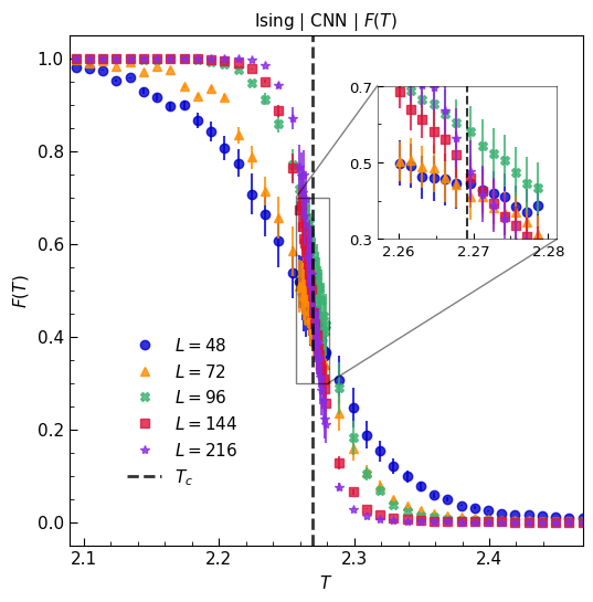
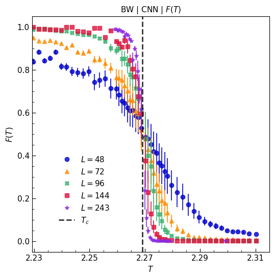
Figure 1: $F^{T}$ ferromagnetic phase predictions for the Ising model (left) and the Baxter-Wu model (right) with FCNN for various lattice sizes. The error bars correspond to the variance $V^{T}$ of the NN prediction. The black vertical dashed line is the position of the critical temperature $T_{c}=2/\ln(1+\sqrt{2})$, which by chance the same for both two models.

For the Ising model, Ref. Carrasquilla and Melko (2017), considered system sizes of up to $L=60$ and observed that the $F^{T}$ curves display data collapse with respect to the “scaling variable”, $tL^{1/\nu}$, where the reduced temperature $t=(T-T_{c})/T$ is scaled by the critical exponent $\nu$. The data collapse estimate of Ref. Carrasquilla and Melko (2017) for $L$ up to $L=60$, produces the values $T_{c}=2.266\pm 0.002$ and $\nu=1.0\pm 0.2$, consistent with the exact values of the critical temperature and the correlation length exponent for the 2D Ising universality class, $\nu{=}1$, Baxter and Wu (1973). Our numerical experiments show that data collapse is visually observed in a wide range of values of the critical exponent $\nu\in[0.75,1.5]$, depending on the network architecture (see Figs 12-23 of Supplemental Materials for details). We stress that simply including larger system sizes does not improve correlation length exponent and critical temperature estimates due to increasing errorbars of the NN output in the critical region, cf Fig.1.

We note however, that the increase of the errobars of $F^{T}$, Eq. (1)—equivalently, the variance $V^{T}$, Eq. (2)—around $T=T_{c}$ is similar to the expected behavior of thermodynamic functions in the critical region, where second moments of observables are related to temperature derivatives of corresponding thermodynamic functions. In this spirit, we consider the second moment of the NN prediction of the FM class, Eq. (2), and hypothesize that the variance of the NN output, Eq. (2) is singular in the thermodynamic limit. This way, the observed increase of the errorbars of $F^{T}$ around $T\approx T_{c}$ is in fact nothing but a finite-size rounding of this divergence, governed by the correlation length exponent $\nu$. Incremental cutoff values are applied to low values of $V(T)$ and $T$ range until the Gaussian fit parameters become stable. The optimal parameters $p_{opt}$ are obtained by minimizing the square deviation $V^{T}_{fit}-V^{T}$ of the non-linear least squares method. With the parameters $p_{opt}$, we estimate the standard deviation $p_{sd}$, which is obtained as a linear approximation of the model function around the optimum Vugrin et al. (2007). We used the built-in functions of the scipy package Virtanen et al. (2020) to get $p_{opt}$, $p_{sd}$.

Fig. 2 displays the temperature dependence of $V^{T}$, which indeed shows a drastic increase around $T=T_{c}$, and a characteristic Gaussian-like bell shape for both Ising and BW models and all network architectures. Furthermore, the widths of the bell-shaped curves decrease with increasing the system size, which is consistent with scaling behavior.

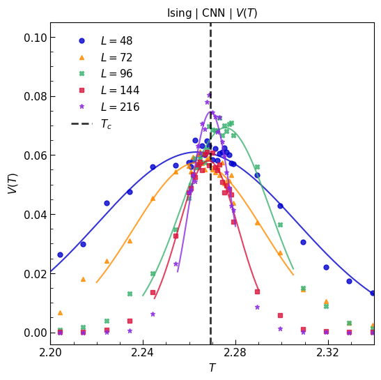
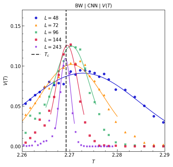
Figure 2: $V^{T}$ variance for the Ising model (left) and the Baxter-Wu model (right) with FCNN for different lattice sizes. The black vertical dahed line is the position of the critical temperature. The solid lines are limited to the area where the Gaussian approximation was applied to extract the width $\sigma$ for each lattice size $L$.

To test this hypothesis, we study the $L$ dependence of the width of the peak of $V^{T}$, Eq. (2). Specifically, for each value of $L$, we fit $V^{T}$ vs T with an unnormalized Gaussian-like Ansatz, $V^{T}\sim\exp\left(-(T-T_{*})^{2}/2\sigma^{2}\right)$, with $\sigma$ and $T_{*}$ being fit parameters, and extract the dependence of the width of $\sigma$ on $L$. Since there is no a priori requirement that the profile is strictly Gaussian, we also perform a separate single-parameter fits the left-hand ($T<T_{*}$) and the right-hand ($T>T_{*}$) parts of the $V^{T}$ curves. In this procedure, $T_{*}$ is simply the location of the maximum of $V^{T}$, and $\sigma$ is the (only) fit parameter. For both fitting protocols, we then fit the resulting widths, $\sigma(L)$, to a power-law Ansatz, $\sigma(L)\sim 1/L^{1/\nu_{\sigma}}$. Similarly to the Gaussian fitting, we obtain the optimal value of $1/\nu_{\sigma}$ and its standard deviation from the power-law fitting. We perform this procedure for the Ising and the BW models and for all network architectures, and results are summarized in Tables 1 and 2.

For the Ising model, Table 1, the first observation is that the resulting values of the scaling exponent (both one-sided $1/\nu_{\sigma}$ and two-sided $1/\nu_{\sigma^{\pm}}$) are consistent with the correlation length exponent for the Ising universality class, $\nu=1$. One notable exception is the ResNet 10- and 34-layer architectures, which shows vastly different values for exponents $1/\nu_{\sigma^{\pm}}$ and $1/\nu_{\sigma}$, and the resulting values are barely within the 4 standard deviations from the exact result, $\nu=1$.

For the BW model, Table 2, the striking observation is that the scaling exponents, $1/\nu_{\sigma}$, estimated from the width of $V^{T}$, are consistent with the exact value of the correlation length exponent for universality class of the BW model, $\nu=2/3$. The accuracy of fit results, Table 2, allows to conclusively distinguish this value from regular, non-singular corrections, $\sim L^{-1}$. This is the major advantage of considering the BW model in addition to the Ising model where $\nu=1$.

We also note that the shape of $V^{T}$ is in fact not symmetric around the maximum—for both Ising and BW models. Allowing for different widths, $\sigma^{+}$ and $\sigma^{-}$ for $T>T_{*}$ and $T<T_{*}$, respectively, produces closer fits of $V^{T}$. Moreover, scaling exponents, $1/\nu_{\sigma^{+}}$ and $1/\nu_{\sigma^{-}}$ are different—the low-temperature exponent, $1/\nu_{\sigma^{-}}$, is consistently larger than the high-temperature exponent, $1/\nu_{\sigma^{+}}$ — again, for both Ising and BW models.

It is clear from Tables 1 and 2 that the values of the critical exponents, extracted from NN data are largely independent of the NN architecture, and that increasing the depth of an NN does not bring drastic improvements in exponent accuracy estimation. For networks of the ResNet family, both for the Ising model and for the BW model, some of the scaling exponents have larger errors than similar ones for simpler architectures FCNN and CNN.

We thus conclude that the width of the $V^{T}$ peak displays finite-size scaling consistent with the universality class of a model, and that simple convolutional networks, CNN, or fully-connected, FCNN, are more appropriate for studying this class of problems, and that increasing the network depth does not automatically translate into better reliability or accuracy of the estimates—this is consistent with the conclusion of Ref. Morningstar and Melko (2018).

Given that the width of the $V^{T}$ peak displays finite size scaling with the correlation length exponent, it is natural to study $L$-dependence of other properties of the peak: its maximum value, $V_{\mathrm{max}}^{T}$, and the shift of the maximum from the thermodynamic limit value of $T_{c}$. Our numerical experiments show that both maximum height and the peak shift are NN architecture dependent and do not display meaningful convergence with $L\to\infty$.

This behavior must be contrasted with the behavior of more traditional thermodynamic observables. It is well known Ferdinand and Fisher (1969) that the position of the specific heat maximum $T^{*}$ shifts from the critical point $T_{C}$ with the correlation length index $T^{*}-T_{C}\propto 1/L^{1/\nu}$, and the same behavior is found for other thermodynamic quantities due to fluctuation cutoff, when the correlation length becomes comparable with the dimensions of the system, similar to i.e. to the rounding of the magnetic susceptibility at a temperature close to the critical one Landau and Binder (2014).

We tested the deviation of the maximum VOT for both models and six networks, and the results are placed in Table 3 for the Ising model and Table 4 for the Baxter-Wu model. Note that the critical temperature values are coincidentally the same for the two models, but $1/\nu$ is different – it is 1 for the Ising model and 1.5 for the Baxter-Wu model, and we use these values when analyzing the VOT data. A demonstration of fits can be found in Supplemental Materials. The results of the fitting are in most cases consistent within no more than five standard deviations and follow the assumption that the shift of the VOT function follows the Ferdinand-Fischer law with an exactly known exponent. The testing of the Ising model with the ResNet-50 network is the worst, and at the same time the $T*$ estimates for the largest systems are very close to the critical temperature $T_{C}$, as can be seen from the Fig. 23 in Supplemental materials. Surprisingly, the values of $T*$ change more regularly with $L^{-1/\nu}$ for the Baxter-Wu model than for the Ising model. This may be due to weaker corrections to scaling for the Baxter-Wu model (see, for discussion Ref. Shchur and Janke (2010)).

NN	$1/\nu_{\sigma}$	$1/\nu_{\sigma^{-}}$	$1/\nu_{\sigma^{+}}$
FCNN	1.01(1)	1.02(13)	0.98(4)
CNN	1.06(3)	1.11(5)	1.07(2)
ResNet-10	1.25(3)	1.24(7)	1.24(3)
ResNet-18	1.17(11)	1.41(6)	1.08(10)
ResNet-34	1.15(16)	1.26(7)	1.12(24)
ResNet-50	1.20(5)	1.21(5)	1.31(6)

Table 1: Peak widths for the Ising model. Here $\nu_{\sigma}$ is the estimate from fitting the Gaussian profile to the $V^{T}$. $\nu_{\sigma}^{+}$ and $\nu_{\sigma}^{-}$ are similar estimates where we only fit the right-hand side (resp., left-hand-side) of the $V^{T}$ curves. See the text for discussion.

NN	$1/\nu_{\sigma}$	$1/\nu_{\sigma^{-}}$	$1/\nu_{\sigma^{+}}$
FCNN	1.49(3)	1.57(2)	1.38(8)
CNN	1.45(5)	1.55(6)	1.49(5)
ResNet-10	1.48(5)	1.65(13)	1.47(4)
ResNet-18	1.32(11)	1.36(14)	1.40(7)
ResNet-34	1.54(6)	1.76(5)	1.47(3)
ResNet-50	1.43(9)	1.69(16)	1.47(5)

Table 2: Peak widths for the Baxter-Wu model. Here $\nu_{\sigma}$, $\nu_{\sigma}^{+}$, and $\nu_{\sigma}^{-}$ are the same as in Table 1.

NN	$T*$	$\Delta/\sigma_{T}$
FCNN	2.2699(5)	1
CNN	2.2727(6)	5
ResNet-10	2.2667(6)	4.2
ResNet-18	2.2688(6)	0.7
ResNet-34	2.2659(6)	5.5
ResNet-50	-	-

Table 3: Ising model: estimation of the critical temperature from the VOT width using Ferdinand-Fisher law. The last column is the difference between the estimated critical temperature and the exact critical temperature $\Delta=|T^{*}-T_{c}|$ divided by the statistical error $\sigma_{T}$ of the weighted linear fit.

NN	$T*$	$\Delta/\sigma_{T}$
FCNN	2.2691(4)	0
CNN	2.2687(4)	1.25
ResNet-10	2.2690(4)	0.25
ResNet-18	2.2684(4)	2
ResNet-34	2.2694(4)	0.5
ResNet-50	2.2688(4)	1

Table 4: Baxter-Wu model: estimation of the critical temperature from the VOT width using Ferdinand-Fisher law. The last column is the difference between the estimated critical temperature and the exact critical temperature $\Delta=|T^{*}-T_{c}|$ divided by the statistical error $\sigma_{T}$ of the weighted linear fit.

Conclusion.— The main result of the presented analysis is that the most reliable information on the classification of snapshots of the spin configuration of statistical mechanics systems experiencing phase transitions of the second kind is contained in the output variation (VOT) of neural networks. Namely, VOT contains information about the critical temperature and the correlation length exponent. We present a VOT analysis method and extract estimates for the critical temperature and correlation length exponent of two systems in two universality classes. The results are stable when using three different architectures in the NN deep pool - CNN, FCNN and Resnet with four configurations.

We do not have theory for the network output function as the thermodynamic function in the same ensemble as the statistical mechanics model which we tested with the neural network. At the same time we found evidence that the VOT width scales with the critical length exponent $\nu$ and demonstrated that clearly for two universality classes. This means that output function $F(T)$ somehow connected to the fluctuation of the physical quantities of the model although the clear connection is not directly found .

We find no evidence that the network output function $F(T)$ should be equal to 1/2 at the critical point, as stated in the pioneering work Carrasquilla and Melko (2017) — our claim is based on careful analysis using different network architecture. Instead, we show that the variation bias of the VOT output function does not contradict the Ferdinand-Fischer picture and can be used to estimate the critical temperature. This estimate is still not under control of the desired accuracy and more work needs to be done on a sound methodology.

We would like to emphasize that the width dependence of VOT on the system size is a good candidate for extracting the exponent $\nu$ of the critical length and gives better accuracy than the approach proposed in Ref. Carrasquilla and Melko (2017) using $F(T)$ collapse data. We should note again that more research is needed to find a reliable way to estimate $\nu$ from the VOT width, since not all network architectures produce $\nu$ with the desired precision.