A Catalog of Distance Determinations for the LAMOST DR8 K Giants in the Galactic Halo

Abstract

We present a catalog of distances for 19, 544 K giants drawn from LAMOST DR8. Most of them are located in the halo of the Milky Way up to $\sim 120$ kpc. There are 15% K giants without SDSS photometry, for which we supplements with Pan-STARRS1 (PS1) photometry calibrated to SDSS photometric system. The possible contamination of the red clumps/horizontal branch are removed according to metallicities and colors before the distance determination. Combining the LAMOST spectroscopic metallicities with the SDSS/PS1 photometry, we estimate the absolute magnitudes in SDSS $r-$band, the distance moduli, and the corresponding uncertainties through an Bayesian approach devised by Xue et al. (2014) for the SEGUE halo K-giants. The typical distance precision is about 11%. The stars in the catalog lie in a region of $4-126$ kpc from the Galactic center, of which with 6, 320 stars beyond 20 kpc and 273 stars beyond 50 kpc, forming the largest spectroscopic sample of distant tracers in the Milky Way halo so far.

1 Introduction

K giants, a kind of luminous stars with typical absolute magnitudes of $-3<M_{r}<1$, are ideal tracers to map the Milky Way halo far beyond the solar neighborhood. For instance, exploring the formation of the Milky Way by quantifying the substructures in the Galactic halo (Starkenburg et al., 2009; Xue et al., 2011; Yang et al., 2019), estimating the total mass of the Milky Way by kinematics of the tracers (Xue et al., 2008), or probing the Milky Way stellar halo profile (Xue et al., 2015; Xu et al., 2018; Thomas et al., 2018), and so on. Good distances and corresponding errors are fundamental to address such interesting and important questions of our Galaxy,

Xue et al. (2014, hereafter X14) devised a Bayesian approach to estimate the distances of the Galactic halo K giant, and applied to SEGUE (the Sloan Extension for Galactic understanding and exploration, Yanny et al., 2009). In X14, three priors are considered, which are the stellar number density profile in the galactic halo, the giant-branch luminosity function, and the different metallicity distributions of the SEGUE K-giant target subclass. Among them, the prior of the luminosity function plays the biggest role in the distance estimates. Neglecting it could cause a systematic bias up to 0.25 mag in distance modulus ($\mathcal{DM}$). Therefore, the Bayesian approach is optimal to get unbiased distance estimates for stars.

Thanks to the huge number of spectra observed in the Large Sky Area Multi-Object Fiber Spectroscopic Telescope (LAMOST, also called the Guo Shou Jing Telescope, Zhao et al., 2006; Cui et al., 2012) and the fact that giants occupy a larger fraction of bright stars, generating a large sample of the halo K giants has been made possible. In this work, adopting the photometry from SDSS and PS1 (defined in Section 2), we estimate the distances and the uncertainties for a large sample of K giants observed in the LAMOST survey by following the Bayesian procedure of X14. Our goal is to present a more complete halo K-giant catalog, including the intrinsic absolute magnitude $M$, heliocentric distance $D$, Galactocentric distance $r_{\rm gc}$ and their corresponding errors as well.

This paper is organized as follows. The data used in this work are introduced in Section 2. The photometry calibration and distance estimation are described in Section 3. The results are shown in Section 4, with a summary in Section 5.

2 Data

K giants which mainly distributed in the Galactic anti-center direction (Yao et al., 2012) is covered by the LAMSOT. LAMOST is a quasi-meridian reflecting Schmidt telescope with an effective aperture of 4 meters and 4000 optical fibers (Cui et al., 2012), from which numerous low-resolution ($R\sim 1800$) spectra covering a wavelength range of $3700<\lambda<9000$ Å of stars with $r<19$ can be obtained simultaneously at one exposure (Zhao et al., 2006, 2012).

We aim to derive distance moduli following the procedure of X14 for K-giant halo stars selected from the LAMOST DR8. With this method, the absolute magnitude of each star is estimated from the empirically calibrated color-magnitude fiducials with metallicities in the range of $-2.38<{\rm[Fe/H]<+0.39}$. The main observables adopted are [Fe/H], $\log g$ and $T_{\rm eff}$ derived from LAMOST stellar spectra, the $g$ and $r$ band magnitudes from the Sloan Digital Sky Survey (SDSS, York et al., 2000) or the Pan-STARRS1 survey (PS1, Chambers & Pan-STARRS Team, 2016). In addition, to eliminate possible red clump stars, 2MASS (Skrutskie et al., 2006) $J$ and $K_{\rm s}$ band magnitudes are also used. Details of the observables are described below.

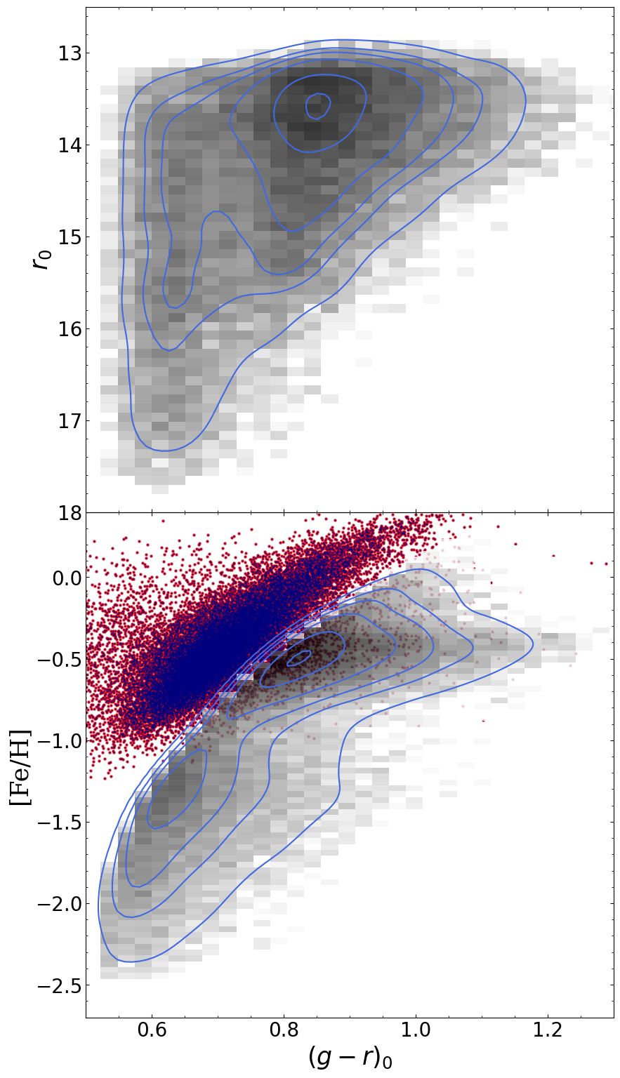
Figure 3: Number density distributions of K-giant sample in the color-magnitude and color-metallicity plane. In the bottom panel, red and dark blue points represent possible RC and HB stars, respectively.

Stellar atmospheric parameters are derived by the official LAMOST Stellar Parameter pipeline (LASP; Wu et al., 2011; Luo et al., 2015), in which the stellar parameters are determined iteratively by minimizing the $\chi^{2}$ between the observed spectrum and the model spectrum from ELODIE stellar library (Prugniel et al., 2007). From all the survey spectra, the K giants used in the study were identified by the selection criteria presented in Liu et al. (2014, Figure 3), that is, $4000<T_{\rm eff}<5600$ K, and $\log g<3.5$ for stars whose $T_{\rm eff}<4600$ K, while $\log g<4.0$ for stars with $4600\leq T_{\rm eff}<5600$ K. It returns $\sim 0.98$ million K giants in LAMOST DR8, including $\sim 16\%$ red clump (RC) giant by using the criterion of Huang et al. (2015), that is,

$$1.8\leq\log g\leq 0.0009\,{\rm dex\,K^{-1}}\{T_{\rm eff}-T^{\rm Ref}_{\rm eff}({\rm[Fe/H]})\}+2.5,$$ (1)

where

$$T^{\rm Ref}_{\rm eff}({\rm[Fe/H]})=-876.8\,{\rm K\,dex^{-1}\,[Fe/H]}+4431\,{\rm K},$$ (2)

and

$$1.21[(J-K_{\rm s})_{0}-0.085]^{9}+0.0011<Z_{\rm metal}<2.58[(J-K_{\rm s})_{0}-0.400]^{3}+0.0034,$$ (3)

where $Z_{\rm metal}$ is converted from [Fe/H] using Eq. 10 of Bertelli et al. (1994), and $(J-K_{\rm s})_{0}$ are photometries taken from 2MASS.

Photometries are firstly adopted from SDSS which use the 2.5 m Sloan Foundation Telescope (Gunn et al., 2006) at Apache Point Observatory (APO). The 16th public data release (DR16; Ahumada et al., 2020) was from the SDSS-IV (Blanton et al., 2017), which contains all prior SDSS $ugriz$ imaging data. (Fukugita et al., 1996; Gunn et al., 1998; York et al., 2000; Stoughton et al., 2002; Pier et al., 2003; Eisenstein et al., 2011; Blanton et al., 2017). For K giants without SDSS photometry, we took the broadband data $grizy_{\rm P1}$ from the second data release (DR2; Flewelling, 2016; Magnier et al., 2020a, b, c; Waters et al., 2020) of PS1 instead, while the Panoramic Survey Telescope and Rapid Response System (Pan-STARRS) is an innovative wide-field astronomical imaging and data processing facility developed at the University of Hawaii’s Institute for Astronomy (Kaiser et al., 2002, 2010). The DR2 of PS1 data used in the present work can be found in MAST: https://doi.org/10.17909/s0zg-jx37 (catalog 10.17909/s0zg-jx37). Finally, there are 45% and 83% stars with SDSS and PS1 photometric data, respectively. Moreover, to select halo K giants with good data quality, only stars whose $E(B-V)$ estimated from Schlegel et al. (1998) and less than 0.25 mag. are adopted. Hence, there are 57% stars left. Then the extinctions in different bandpass were calculated by Fitzpatrick (1999) reddening law with measurements of Schlafly & Finkbeiner (2011).

3 Photometry Calibration and Distance Estimates

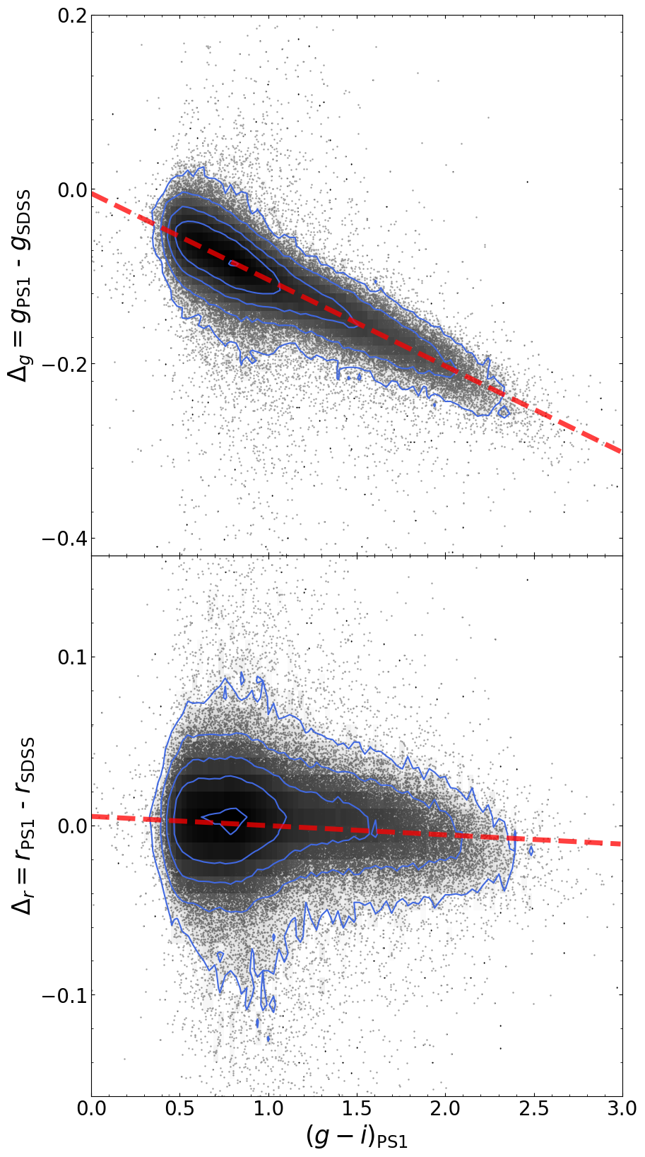
Figure 1: Apparent magnitude difference between PS1 and SDSS as functions of PS1 color $(g-i)_{\rm PS1}$ for the mags of $g$ and $r$. Density distributions in $\Delta$ – color spaces are shown. Red dashed lines represent the best fit to the data.

For stars without SDSS photometry, the PS1 data is taken as a complement. From common stars both observed by SDSS and PS1, trends in the difference between the PS1 and SDSS photometry $\Delta_{m}=m_{\rm PS1}-m_{\rm SDSS}$ with PS1 colors $(g-i)_{\rm PS1}$ can be found (see Figure 1). Thus, we need to remove the trends by calibrating the PS1 photometry to match the SDSS one before distance estimates.

Here we perform the calibration by fitting an empirical curve to $\Delta_{m}$, where $m$ represents apparent magnitudes $g$ and $r$, as a function of PS1 color $(g-i)$, and thus adjusting the PS1 photometry. To model $\Delta_{m}-(g-i)$ precisely, we chose stars both observed by SDSS and PS1 in the apparent magnitude ranges of $13.<g_{\rm SDSS}<22.2$, $13.<r_{\rm SDSS}<22.2$, $13.<i_{\rm SDSS}<21.3$, $13.<g_{\rm PS1}<22$, $13.<r_{\rm PS1}<21.8$, and $13.<i_{\rm PS1}<21.5$, with small observation uncertainties, that is, $\sigma_{m}<0.05$ ($m=g,r,i$). It results 168, 887 common stars used for the present calibration.

We find the best fit slopes of lines in $\Delta_{m}$ vs. $(g-i)_{\rm PS1}$ space with least absolute deviation line fitting, which minimizes the absolute value of the residuals,

$$\sum_{j}|\Delta_{m,j}-F_{m}((g-i)_{{\rm PS1},j})|,$$ (4)

to exclude outliers. The standard errors of the fitted slopes are estimated via bootstrapping. Figure 1 shows the best fits in $\Delta_{m}-(g-i)_{\rm PS1}$ space, the fittings are:

$$\Delta_{g}= \,\,(-0.0050\pm 1.0\times 10^{-4})\,+\,$$ (5)

$$\,\,(-0.0099\pm 7.1\times 10^{-5})\times(g-i)_{\rm PS1},$$

and

$$\Delta_{r}= \,\,(0.0054\pm 2.1\times 10^{-4})\,+\,$$ (6)

$$\,\,(-0.0055\pm 1.5\times 10^{-4})\times(g-i)_{\rm PS1}.$$

The calibrated results are shown in Figure 2. The upper panels present that the calibrated $g_{\rm PS1}$ and $r_{\rm PS1}$ show very good consistency with the SDSS photometry. In the lower panels, it can be seen that the mean values of adjusted $\Delta_{m}$ are 0.0 with standard errors of 0.025 and 0.023 for $g$ and $r$ mags, respectively, which proves the validity of the calibration in this work.

With the calibrated results, we converted PS1 photometries to SDSS ones for stars without SDSS observation. Finally, we obtains 375, 585 stars with $g_{0}$, $r_{0}$, $i_{0}$, and $E(B-V)<0.25$. The present distance measurement is for halo stars only. Therefore, we selected halo K giants preliminarily before the distance measurements. Considering the colors and metallicities of used giant-branch fiducials of clusters, only K giants whose ${\rm[Fe/H]<+0.39}$ and $0.5\leq(g-r)_{0}\leq 1.4$ are taken. We further excluded stars labeled as RC and stars below the level of the horizontal branch (BH) by using a quadratic polynomial of $(g-r)_{0}^{\rm HB}={\rm 0.087[Fe/H]^{2}+0.39[Fe/H]+0.96}$, which is fitted by X14, since the red HB as well as the RC in a cluster have the same color as K giants, but quite different absolute magnitudes, which in the end leaves 42, 713 stars. Figure 3 shows the number density distribution of K giants in $r_{0}$ vs. $(g-r)_{0}$ and [Fe/H] vs. $(g-r)_{0}$ spaces. It can be notice that partial RC stars overlap with K giants, since the Galactic halo contains metal-rich substructures(Yang et al., 2019).

We then implemented a Bayesian approach to derive the posterior PDF of $\mathcal{DM}$ for each K giant, and hence to provide both a distance estimate and its uncertainty. According to X14, the relative probability of different $\mathcal{DM}$ is defined as

$$P(\mathcal{DM}|\{m,c,{\rm[Fe/H]}\})= \frac{P(\{m,c,{\rm[Fe/H]}\}|\mathcal{DM})}{P(\{m,c,{\rm[Fe/H]}\})}$$ (7)

$$\times p_{\rm prior}(\mathcal{DM}),$$

where $P(\{m,c,{\rm[Fe/H]}\})$ is a non-zero constant of normalization, $p_{\rm prior}(\mathcal{DM})$ is the prior probability for the $\mathcal{DM}$. It reflects any information on the stellar number density which follows a power law $\nu(r)=r^{\alpha}$ in the Galactic halo, where $\alpha\in(-4,-2)$ (Bell et al., 2008). With mock data, X14 has proved that the variances in the final estimated $\mathcal{DM}$ caused by $p_{\rm prior}(\mathcal{DM})$ can be neglected if $\alpha$ values are in $(-4,-2)$. $P(\{m,c,{\rm[Fe/H]}\}|\mathcal{DM})$ is the likelihood of $\mathcal{DM}$, e.g., $\mathscr{L}(\mathcal{DM})$, in which prior information of the giant-branch luminosity function $p_{\rm prior}(M)$ and the metallicity distribution of halo giants $p_{\rm prior}({\rm[Fe/H]})$ are involved, that is,

$$\mathscr{L}(\mathcal{DM})= \int\int p(\{m,c,{\rm[Fe/H]}|\mathcal{DM},M,{\rm[Fe/H]}\})$$ (8)

$$\times p_{\rm prior}(M)p_{\rm prior}({\rm[Fe/H]})dMd{\rm[Fe/H]}.$$

$p_{\rm prior}(M)\propto 10^{0.32M}$ is derived from the observed luminosity functions of the giant branch of global clusters M 5 (${\rm[Fe/H]}=-1.4$, Sandquist et al., 1996) and M 30 (${\rm[Fe/H]}=-2.13$, Sandquist et al., 1999), and the Basti theoretical ones with ${\rm[Fe/H]}=-2.4$ and ${\rm[Fe/H]}=0.0$ (Pietrinferni et al., 2004). $p_{\rm prior}({\rm[Fe/H]})$ is from metallicity distribution of the K-giants.

To calculate $\mathscr{L}(\mathcal{DM})$, the colors at a given $M$ and [Fe/H], $c(M,{\rm[Fe/H]})$, need to be predicted first. The value is interpolated from a set of empirical giant-branch fiducials of $(g-r)_{0}$ - $M_{r}$, which adopted from the globular clusters M 92, M 13, and M 71, the open cluster NGC 6791, and the Basti $\alpha-$enhanced isochrones (Pietrinferni et al., 2006). $\alpha$ abundance also plays an important role in $c(M,{\rm[Fe/H]})$ determination, e.g., at the same [Fe/H] values, the difference of $r$-band absolute magnitude can be as large as 0.5 mag at the tip of the giant branch between an $\alpha$-enhanced giant and a solar-scaled $\alpha$-abundance one (X14). However, in the Galactic halo, a few K giants are metal-rich with poor [$\alpha$/Fe], such as K giants which are belong to Sagittarius Stream (Yang et al., 2019). In this situation, for the K giants with $0.<{\rm[Fe/H]}<+0.39$, the $\alpha$ abundances are assumed to be gradually weakening between solar and the NGC 6791 value, while for normal $\alpha$-enhanced metal-poor halo stars, the cluster fiducial and one isochrone are used.

For more details of the distance calculation procedure, we refer the readers to X14, and reference therein. Finally, the best estimates of the distance moduli and their errors are given by the median and central 68% interval of $\mathscr{L}(\mathcal{DM})$.

4 Results

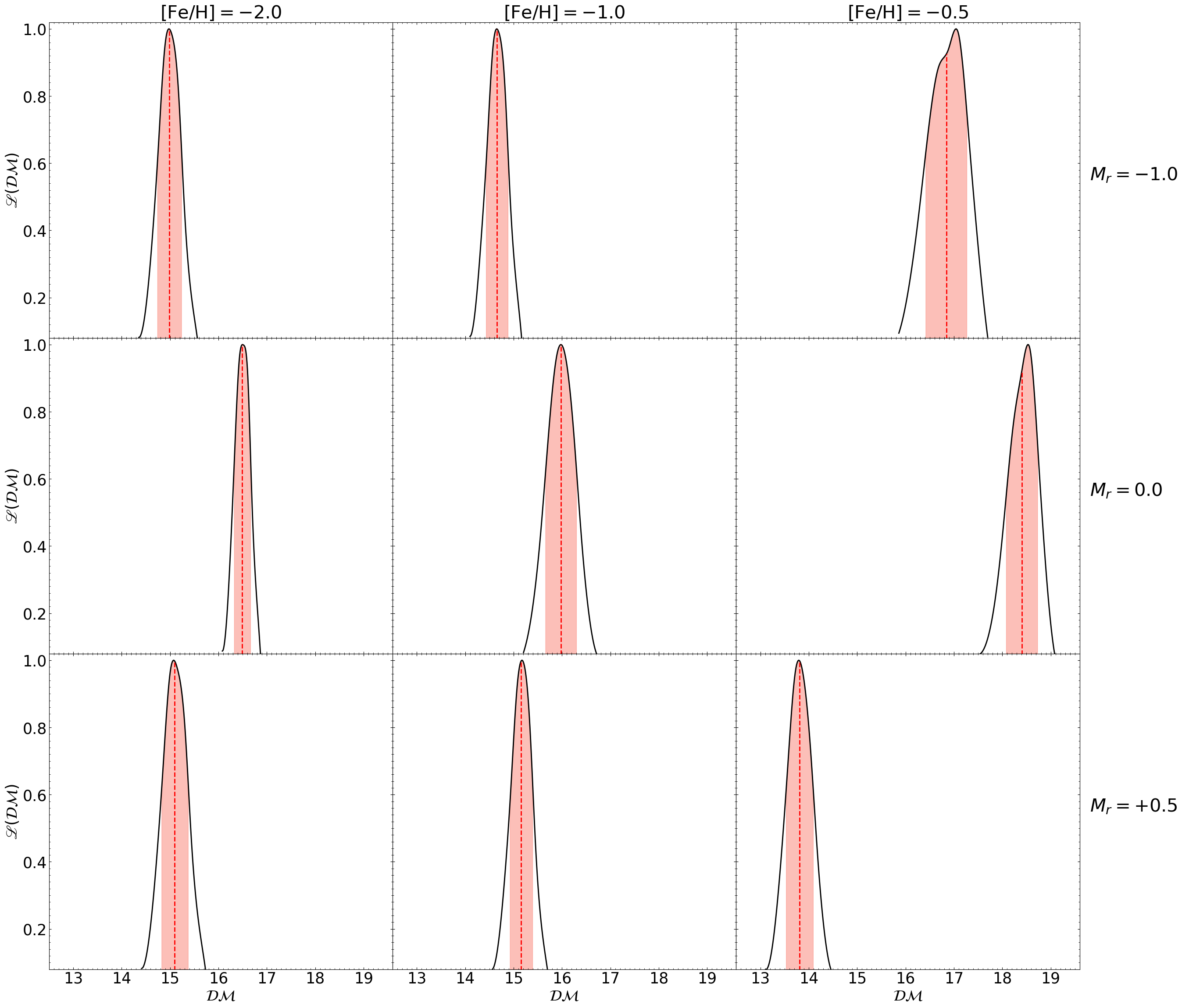
Figure 4: Typical $\mathscr{L}(\mathcal{DM})$ for stars with different [Fe/H] and $M_{r}$. In each plot, the black thick line represents the most likely $\mathcal{DM}$. The red dashed line and the shade indicate the median value and 68% interval, respectively.

Figure 4 shows examples of the $\mathcal{DM}$ estimates and corresponding uncertainties from $P(\mathcal{DM}|\{m,c,{\rm[Fe/H]}\})$. Meanwhile, the absolute magnitudes, $M_{r}(=r_{0}-\mathcal{DM}_{\rm median})$, distances ($D$) from the Sun, Galactocentric distances ($r_{\rm gc}$), positions ($[x,y,z]$) in the Galacticcentric Cartesian coordinate system by adopting $R_{\odot}=8.34$ kpc (Reid et al., 2014) are obtained. To generate reliable catalog for the Galactic halo K giants, we first exclude disk stars and the K giants with bad distance estimates through the criteria of $|z|>5.$ kpc, ${\rm[Fe/H]}<-1.0$ if $2.~{}{\rm kpc}<|z|<5.$ kpc, and $\sigma_{\rm D}/{\rm D}<0.3$. Then we calculate the kinematic parameters by combining proper motions from Gaia Early Data Release 3 (EDR3; Gaia Collaboration et al., 2016, 2021), and hence the total energy for the rest stars to make sure the given K giants are bound to the Milky Way, which weeds out 665 stars. Finally, It results a catalog of 19, 544 halo K giants. The main entries in the catalog are the best estimates of the distance moduli and their uncertainties ($\mathcal{DM}_{\rm median}$, $\sigma_{\mathcal{DM}}$), the heliocentric distances and their errors (${\rm D}$, $\sigma_{\rm D}$), the Galactocentric distances and their errors ($r_{\rm gc}$, $\sigma_{r_{\rm gc}}$), the absolute magnitudes in $r-$band and the corresponding errors ($M_{r}$, $\sigma_{M_{r}}$), and the $\mathcal{DM}$ at (5%, 16%, 50%, 84%, 95%) confidence of $\mathscr{L}(\mathcal{DM})$. These values and other parameters are all included in Table 1. The complete version of this table is available in the online version.

The overall properties of the ensemble of distance estimates are shown in Figure 5. It can be seen that the average precisions in both of $M_{r}$ and $\mathcal{DM}$ are 0.32 mags, and the faint giants have less precise in $M_{r}$ estimates. The mean relative error in distance, $\sigma_{\rm D}/{\rm D}$, is 0.145, and the present K giants can reach as far as 120 kpc with very good precisions (e.g., $\sigma_{\rm D}/{\rm D}<0.15$). The distance results of fractional nearby stars are less precise because they tend to be on the steep part of the giant branch in the CMD, especially for stars in low metallicity range. Figure 6 shows the number density and $\sigma_{M_{r}}$ distribution of halo K giants in the CMD. More stars gather in the lower part of the giant branch, which is consistent with the prediction of the luminosity function. The precision of the distance is increasing along with the red-giant branch, that is, stars in the upper part of the RGB have more precise distances than those in the lower part because the fiducials are much steeper near the sub-giant branch. This characters is consistent with the distance estimates of SEGUE K giants in X14. Moreover, we compare the present estimates with ones in X14 for 795 common stars in Figure 7. In this figure, both peak values ($\mathcal{DM}_{\rm peak}$) and $\mathcal{DM}$ at 50% of $\mathscr{L}(\mathcal{DM})$ are shown. The standard deviations are 0.29 and 0.28 for $\Delta_{\mathcal{DM}_{\rm peak}}$ and $\Delta_{\mathcal{DM}_{50}}$, respectively. It can be seen that the two estimates show good consistency and the $\Delta_{\mathcal{DM}}$ values are independent of the estimated $\mathcal{DM}$, which proves the applicability of this approach to the LAMOST data. The scatter is mainly caused by different input [Fe/H] values used in the distance estimates.

Figure 8 presents the number density and $\sigma_{\rm D}/{\rm D}$ in $R_{\rm GC}-|z|$ plane. Our sample of K giants lies in the region of $4-126$ kpc from the Galactic center. In the sample, 6, 320 stars are in the region of $r_{\rm gc}>20$ kpc, including 221 stars in $52<r_{\rm gc}<80$ kpc and 68 stars whose $r_{\rm gc}$ are larger than 80 kpc. The sample size is as double as SEGUE K giants in X14. The large sample can help us to trace the mass density for both of the Galactic inner and outer halos in the following works.

To check the validation of our distance estimates in this work, we also compare our results with the parallaxes adopted from Gaia EDR3. Only stars in $\sigma_{\varpi}/\varpi<0.1$ and $\sigma_{\rm D}/{\rm D}<0.15$ are taken, which results 5, 497 K giants. The comparison result is shown in Figure 9, in which our distance estimates show very good consistency with parallaxes from Gaia EDR3 catalog for stars with precise parallax measurements.

5 Summary

We have selected the K giants from LAMSOT DR8, excluding red clumps and stars below the horizontal branch carefully. After calibrating the PS1 photometry $gi_{\rm PS1}$ to the $gr_{\rm SDSS}$ of SDSS DR16, we combined the $gr$ with the [Fe/H] from LAMOST LASP, to estimate intrinsic absolute magnitudes in $r-$band, $\mathcal{DM}$, the distances, and the corresponding uncertainties through an Bayesian approach for the K giants. The priors adopted in this work are the giant-branch luminosity function derived from globular clusters, and the metallicity distributions from the present K-giant sample. The predicted colors $c(M_{r},{\rm[Fe/H]})$, are obtained from empirical color-magnitude fiducials from old stellar clusters, the best estimates of the distance moduli and their errors can be estimated using the median value and central 68% interval of $\mathscr{L}(\mathcal{DM})$. The mean relative distance error is 0.145, and the distance errors of stars which lie on the lower part of the giant branch in the CMD are relative larger. With the estimated distances and their errors, we selected halo K giants in the ranges of $|z|>5.$ kpc, ${\rm[Fe/H]}<-1.0$ if $2.~{}{\rm kpc}<|z|<5.$ kpc, and $\sigma_{\rm D}/{\rm D}<0.3$. After excluding stars are not bound by the Galactic potential, it results 19, 544 halo K giants, which is three times larger than the number of X14 from SEGUE K giants. In the catalog, 6, 320 stars are in the region of $r_{\rm gc}>20$ kpc, including 221 stars in $50<r_{\rm gc}<80$ kpc and 52 stars whose $r_{\rm gc}$ are larger than 80 kpc. Furthermore, we compared the distances with parallaxes from Gaia EDR3 catalog for stars with precise parallax measurements. The result presents a very good consistency, which proves the validation of the estimates in this work.

We finally present an online catalog containing the $\mathcal{DM}$, and LASP atmospheric parameters for the 19, 544 halo K giants. For each object in the catalog, we also list the basic observables such as (R.A., Dec.), extinction corrected apparent magnitudes and de-reddened colors, and heliocentric radial velocities from LAMOST. The Bayesian estimates of the $\mathcal{DM}$, heliocentric distance, Galactocentric distances, the absolute magnitudes and their uncertainties, along with the $\mathcal{DM}$ at [5%, 16%, 50%, 84%, 95%] confidence of $\mathscr{L}(\mathcal{DM})$.

.

Figure 2: Calibration results. The upper panels show adjusted PS1 photometry. Red dashed lines are diagonals. The lower panels present PDFs of $\Delta_{m}$ after calibration. The mean values and 68% intervals are shown in red lines and shades, respectively.

Figure 5: Distance results for 19, 544 halo K giants. The density distribution maps of the absolute magnitudes in $r-$band, $\mathcal{DM}$, and distance vs. their corresponding uncertainties are presented from upper to bottom panels, respectively.

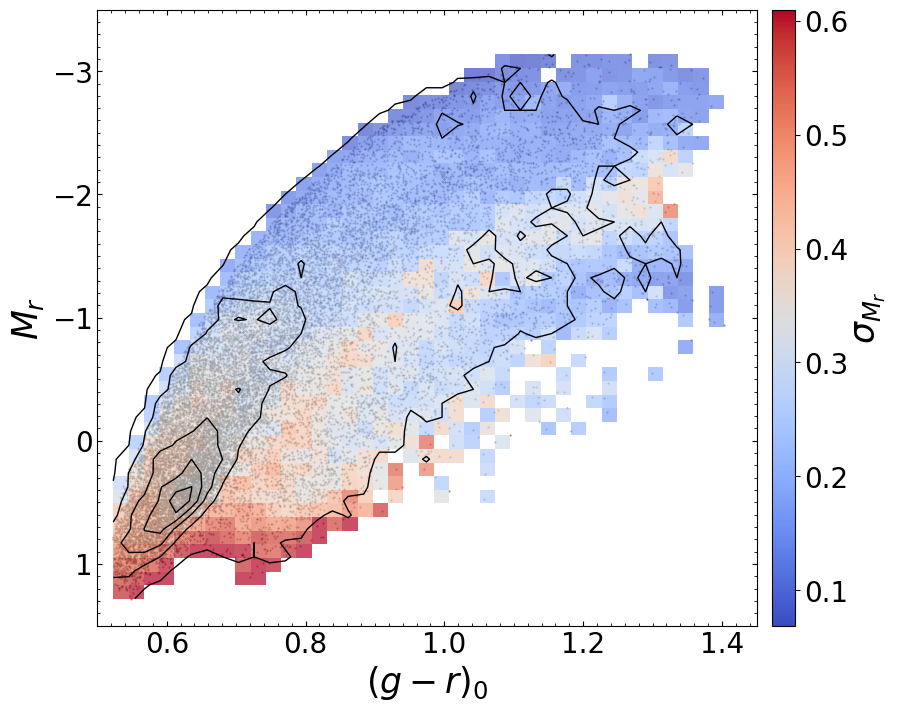
Figure 6: The errors of the absolute magnitude of $r-$band, $\sigma_{M_{r}}$ as a function of $M_{r}$ and $(g-r)_{0}$. Black contours are the density distribution of $M_{r}-(g-r)_{0}$ plane.

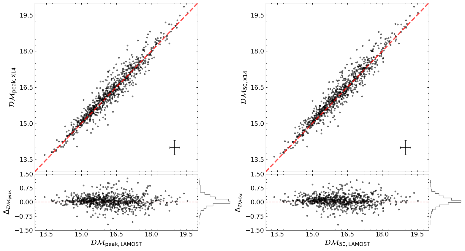
Figure 7: Distance comparison for 795 common stars between the present catalogue and the one in X14. The peak values, and $\mathcal{DM}$ at 50% of $\mathscr{L}(\mathcal{DM})$ are shown in the left and right panels, respectively. Diagonals and values of $\Delta_{\mathcal{DM}}=0.$ are shown in red dashed lines. Note that $\Delta_{\mathcal{DM}}=\mathcal{DM}_{\rm X14}-\mathcal{DM}_{\rm LAMOST}$ for both of the lower panels.

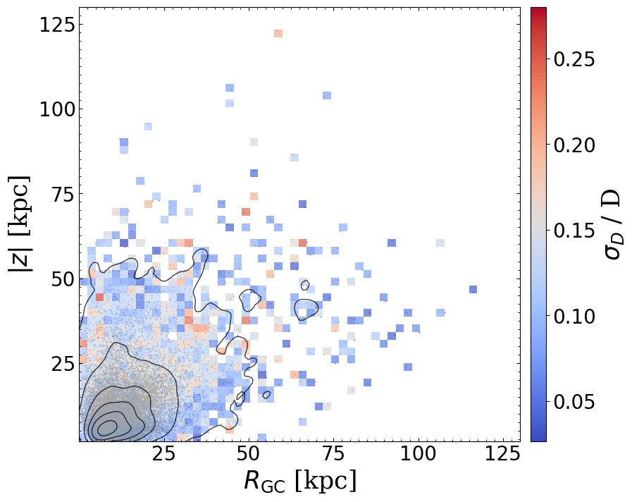
Figure 8: The number and $\sigma_{\rm D}$ / D distributions in $R_{\rm GC}-|z|$ plane for the halo K giants. The stars can trace as far as $R_{\rm GC}=125$ kpc with good precisions.

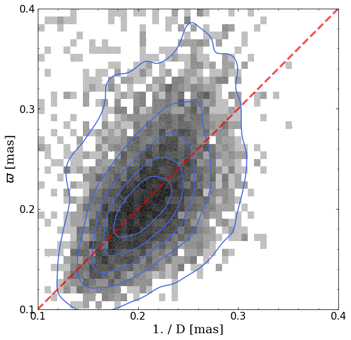
Figure 9: Our distances of good estimates ($\sigma_{\rm D}/{\rm D}<0.15$) compare with parallaxes whose relative errors $\sigma_{\varpi}/\varpi<0.1$ from Gaia EDR3. Red dashed lines are diagonals.

Table 1: Catalog of 19, 544 K Giants Selected from LAMOST DR8

R.A. (J2000)	Dec. (J2000)	$r_{0}$	$\sigma_{r_{0}}$	$(g-r)_{0}$	$\sigma_{(g-r)_{0}}$	RV	$\sigma_{\rm RV}$	$T_{\rm eff}$	$\sigma_{T_{\rm eff}}$	$\log g$	$\sigma_{\log g}$	[Fe/H]	$\sigma_{\rm[Fe/H]}$	$\mathcal{DM}_{5\%}$	$\mathcal{DM}_{16\%}$	$\mathcal{DM}_{50\%}$	$\mathcal{DM}_{84\%}$	$\mathcal{DM}_{95\%}$	$\sigma_{\mathcal{DM}}$	$M_{r}$	$\sigma_{M_{r}}$	$D$	$\sigma_{D}$	$r_{\rm gc}$	$\sigma_{r_{\rm gc}}$
$M_{r}$	$\sigma_{M_{r}}$	$D$	$\sigma_{D}$	$r_{\rm gc}$	$\sigma_{r_{\rm gc}}$
[deg]	[deg]	[mag]	[mag]	[mag]	[mag]	[${\rm km\,s^{-1}}$]	[${\rm km\,s^{-1}}$]	[K]	[K]	[dex]	[dex]	[dex]	[dex]	[mag]	[mag]	[mag]	[mag]	[mag]	[mag]	[mag]	[mag]	[kpc]	[kpc]	[kpc]	[kpc]
272.152	38.854	14.853	0.037	1.071	0.018	-111.2	3.8	4137.0	41.0	1.90	0.07		0.04	15.48	15.61	15.79	15.97	16.08	0.18	-0.94	0.19	14.38	1.21	13.59	1.01
232.282	41.214	13.324	0.037	1.161	0.017	-161.6	3.9	4027.0	51.0	1.80	0.09		0.05	14.27	14.38	14.53	14.68	14.80	0.15	-1.21	0.16	8.06	0.56	9.99	0.35
187.613	29.159	14.306	0.040	0.827	0.035	-99.9	4.8	4476.0	47.0	2.61	0.08		0.04	13.87	14.07	14.37	14.66	14.84	0.30	-0.06	0.30	7.45	1.02	11.40	0.73
214.504	14.421	13.593	0.040	1.227	0.032	45.3	3.7	3851.0	59.0	1.77	0.10		0.06	14.44	14.57	14.74	14.88	14.97	0.15	-1.13	0.16	8.82	0.63	9.22	0.38
222.955	19.915	14.372	0.039	1.059	0.028	-115.0	3.9	4119.0	42.0	1.87	0.07		0.04	14.91	15.04	15.25	15.45	15.57	0.20	-0.87	0.20	11.20	1.04	10.58	0.76

References

- Ahumada et al. (2020) Ahumada, R., Prieto, C. A., Almeida, A., et al. 2020, ApJS, 249, 3, doi: 10.3847/1538-4365/ab929e
- Bell et al. (2008) Bell, E. F., Zucker, D. B., Belokurov, V., et al. 2008, ApJ, 680, 295, doi: 10.1086/588032
- Bertelli et al. (1994) Bertelli, G., Bressan, A., Chiosi, C., Fagotto, F., & Nasi, E. 1994, A&AS, 106, 275
- Blanton et al. (2017) Blanton, M. R., Bershady, M. A., Abolfathi, B., et al. 2017, AJ, 154, 28, doi: 10.3847/1538-3881/aa7567
- Chambers & Pan-STARRS Team (2016) Chambers, K. C., & Pan-STARRS Team. 2016, in American Astronomical Society Meeting Abstracts, Vol. 227, American Astronomical Society Meeting Abstracts #227, 324.07
- Cui et al. (2012) Cui, X.-Q., Zhao, Y.-H., Chu, Y.-Q., et al. 2012, Research in Astronomy and Astrophysics, 12, 1197, doi: 10.1088/1674-4527/12/9/003
- Eisenstein et al. (2011) Eisenstein, D. J., Weinberg, D. H., Agol, E., et al. 2011, AJ, 142, 72, doi: 10.1088/0004-6256/142/3/72
- Fitzpatrick (1999) Fitzpatrick, E. L. 1999, PASP, 111, 63, doi: 10.1086/316293
- Flewelling (2016) Flewelling, H. 2016, in American Astronomical Society Meeting Abstracts, Vol. 227, American Astronomical Society Meeting Abstracts #227, 144.25
- Fukugita et al. (1996) Fukugita, M., Ichikawa, T., Gunn, J. E., et al. 1996, AJ, 111, 1748, doi: 10.1086/117915
- Gaia Collaboration et al. (2016) Gaia Collaboration, Prusti, T., de Bruijne, J. H. J., et al. 2016, A&A, 595, A1, doi: 10.1051/0004-6361/201629272
- Gaia Collaboration et al. (2021) Gaia Collaboration, Brown, A. G. A., Vallenari, A., et al. 2021, A&A, 649, A1, doi: 10.1051/0004-6361/202039657
- Gunn et al. (1998) Gunn, J. E., Carr, M., Rockosi, C., et al. 1998, AJ, 116, 3040, doi: 10.1086/300645
- Gunn et al. (2006) Gunn, J. E., Siegmund, W. A., Mannery, E. J., et al. 2006, AJ, 131, 2332, doi: 10.1086/500975
- Huang et al. (2015) Huang, Y., Liu, X.-W., Zhang, H.-W., et al. 2015, Research in Astronomy and Astrophysics, 15, 1240, doi: 10.1088/1674-4527/15/8/010
- Kaiser et al. (2002) Kaiser, N., Aussel, H., Burke, B. E., et al. 2002, in Society of Photo-Optical Instrumentation Engineers (SPIE) Conference Series, Vol. 4836, Survey and Other Telescope Technologies and Discoveries, ed. J. A. Tyson & S. Wolff, 154–164, doi: 10.1117/12.457365
- Kaiser et al. (2010) Kaiser, N., Burgett, W., Chambers, K., et al. 2010, in Society of Photo-Optical Instrumentation Engineers (SPIE) Conference Series, Vol. 7733, Ground-based and Airborne Telescopes III, ed. L. M. Stepp, R. Gilmozzi, & H. J. Hall, 77330E, doi: 10.1117/12.859188
- Liu et al. (2014) Liu, C., Deng, L.-C., Carlin, J. L., et al. 2014, ApJ, 790, 110, doi: 10.1088/0004-637X/790/2/110
- Luo et al. (2015) Luo, A. L., Zhao, Y.-H., Zhao, G., et al. 2015, Research in Astronomy and Astrophysics, 15, 1095, doi: 10.1088/1674-4527/15/8/002
- Magnier et al. (2020a) Magnier, E. A., Schlafly, E. F., Finkbeiner, D. P., et al. 2020a, ApJS, 251, 6, doi: 10.3847/1538-4365/abb82a
- Magnier et al. (2020b) Magnier, E. A., Sweeney, W. E., Chambers, K. C., et al. 2020b, ApJS, 251, 5, doi: 10.3847/1538-4365/abb82c
- Magnier et al. (2020c) Magnier, E. A., Chambers, K. C., Flewelling, H. A., et al. 2020c, ApJS, 251, 3, doi: 10.3847/1538-4365/abb829
- Pier et al. (2003) Pier, J. R., Munn, J. A., Hindsley, R. B., et al. 2003, AJ, 125, 1559, doi: 10.1086/346138
- Pietrinferni et al. (2004) Pietrinferni, A., Cassisi, S., Salaris, M., & Castelli, F. 2004, ApJ, 612, 168, doi: 10.1086/422498
- Pietrinferni et al. (2006) —. 2006, ApJ, 642, 797, doi: 10.1086/501344
- Prugniel et al. (2007) Prugniel, P., Koleva, M., Ocvirk, P., Le Borgne, D., & Soubiran, C. 2007, in Stellar Populations as Building Blocks of Galaxies, ed. A. Vazdekis & R. Peletier, Vol. 241, 68–72, doi: 10.1017/S1743921307007454
- Reid et al. (2014) Reid, M. J., Menten, K. M., Brunthaler, A., et al. 2014, ApJ, 783, 130, doi: 10.1088/0004-637X/783/2/130
- Sandquist et al. (1999) Sandquist, E. L., Bolte, M., Langer, G. E., Hesser, J. E., & de Oliveira, C. M. 1999, ApJ, 518, 262, doi: 10.1086/307268
- Sandquist et al. (1996) Sandquist, E. L., Bolte, M., Stetson, P. B., & Hesser, J. E. 1996, ApJ, 470, 910, doi: 10.1086/177920
- Schlafly & Finkbeiner (2011) Schlafly, E. F., & Finkbeiner, D. P. 2011, ApJ, 737, 103, doi: 10.1088/0004-637X/737/2/103
- Schlegel et al. (1998) Schlegel, D. J., Finkbeiner, D. P., & Davis, M. 1998, ApJ, 500, 525, doi: 10.1086/305772
- Skrutskie et al. (2006) Skrutskie, M. F., Cutri, R. M., Stiening, R., et al. 2006, AJ, 131, 1163, doi: 10.1086/498708
- Starkenburg et al. (2009) Starkenburg, E., Helmi, A., Morrison, H. L., et al. 2009, ApJ, 698, 567, doi: 10.1088/0004-637X/698/1/567
- Stoughton et al. (2002) Stoughton, C., Lupton, R. H., Bernardi, M., et al. 2002, AJ, 123, 485, doi: 10.1086/324741
- Thomas et al. (2018) Thomas, G. F., McConnachie, A. W., Ibata, R. A., et al. 2018, MNRAS, 481, 5223, doi: 10.1093/mnras/sty2604
- Waters et al. (2020) Waters, C. Z., Magnier, E. A., Price, P. A., et al. 2020, ApJS, 251, 4, doi: 10.3847/1538-4365/abb82b
- Wu et al. (2011) Wu, Y., Luo, A. L., Li, H.-N., et al. 2011, Research in Astronomy and Astrophysics, 11, 924, doi: 10.1088/1674-4527/11/8/006
- Xu et al. (2018) Xu, Y., Liu, C., Xue, X.-X., et al. 2018, MNRAS, 473, 1244, doi: 10.1093/mnras/stx2361
- Xue et al. (2015) Xue, X.-X., Rix, H.-W., Ma, Z., et al. 2015, ApJ, 809, 144, doi: 10.1088/0004-637X/809/2/144
- Xue et al. (2008) Xue, X. X., Rix, H. W., Zhao, G., et al. 2008, ApJ, 684, 1143, doi: 10.1086/589500
- Xue et al. (2011) Xue, X.-X., Rix, H.-W., Yanny, B., et al. 2011, ApJ, 738, 79, doi: 10.1088/0004-637X/738/1/79
- Xue et al. (2014) Xue, X.-X., Ma, Z., Rix, H.-W., et al. 2014, ApJ, 784, 170, doi: 10.1088/0004-637X/784/2/170
- Yang et al. (2019) Yang, C., Xue, X.-X., Li, J., et al. 2019, ApJ, 886, 154, doi: 10.3847/1538-4357/ab48e2
- Yanny et al. (2009) Yanny, B., Rockosi, C., Newberg, H. J., et al. 2009, AJ, 137, 4377, doi: 10.1088/0004-6256/137/5/4377
- Yao et al. (2012) Yao, S., Liu, C., Zhang, H.-T., et al. 2012, Research in Astronomy and Astrophysics, 12, 772, doi: 10.1088/1674-4527/12/7/005
- York et al. (2000) York, D. G., Adelman, J., Anderson, John E., J., et al. 2000, AJ, 120, 1579, doi: 10.1086/301513
- Zhao et al. (2006) Zhao, G., Chen, Y.-Q., Shi, J.-R., et al. 2006, Chinese J. Astron. Astrophys., 6, 265, doi: 10.1088/1009-9271/6/3/01
- Zhao et al. (2012) Zhao, G., Zhao, Y.-H., Chu, Y.-Q., Jing, Y.-P., & Deng, L.-C. 2012, Research in Astronomy and Astrophysics, 12, 723, doi: 10.1088/1674-4527/12/7/002
.