Bayesian Reinforcement Learning with Limited Cognitive Load
Abstract
All biological and artificial agents must learn and make decisions given limits on their ability to process information. As such, a general theory of adaptive behavior should be able to account for the complex interactions between an agent’s learning history, decisions, and capacity constraints. Recent work in computer science has begun to clarify the principles that shape these dynamics by bridging ideas from reinforcement learning, Bayesian decision-making, and rate-distortion theory. This body of work provides an account of capacity-limited Bayesian reinforcement learning, a unifying normative framework for modeling the effect of processing constraints on learning and action selection. Here, we provide an accessible review of recent algorithms and theoretical results in this setting, paying special attention to how these ideas can be applied to studying questions in the cognitive and behavioral sciences.
Keywords: Bayesian decision making, Efficient exploration, Reinforcement learning, Multi-armed bandits, Information theory, Rate-distortion theory
1 Introduction
Cognitive science aims to identify the principles and mechanisms that underlie adaptive behavior. An important part of this endeavor is the development of unifying, normative theories that specify “design principles” that guide or constrain how intelligent systems respond to their environment (Marr, 1982; Anderson, 1990; Lewis et al., 2014; Griffiths et al., 2015; Gershman et al., 2015). For example, accounts of learning, cognition, and decision-making often posit a function that an organism is optimizing—e.g., maximizing long-term reward or minimizing prediction error—and test plausible algorithms that achieve this—e.g., a particular learning rule or inference process. Historically, normative theories in cognitive science have been developed in tandem with new formal approaches in computer science and statistics. This partnership has been fruitful even given differences in scientific goals (e.g., engineering artificial intelligence versus reverse-engineering biological intelligence). Normative theories play a key role in facilitating cross-talk between different disciplines by providing a shared set of mathematical, analytical, and conceptual tools for describing computational problems and how to solve them (Ho and Griffiths, 2022).
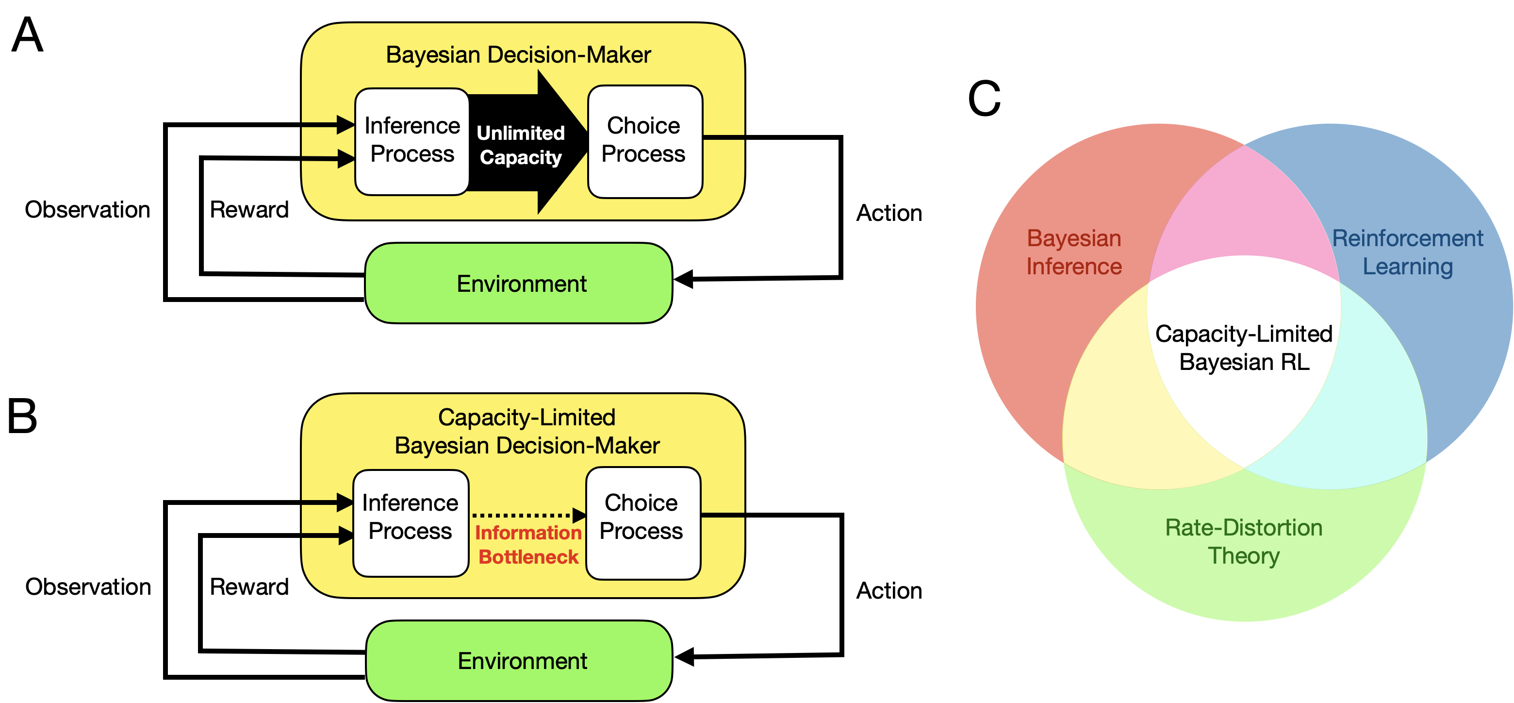
This paper is written in the spirit of such cross-disciplinary fertilization. Here, we review recent work in computer science (Arumugam and Van Roy, 2021a, 2022) that develops a novel approach for unifying three distinct mathematical frameworks that will be familiar to many cognitive scientists (Figure 1). The first is Bayesian inference, which has been used to study a variety of perceptual and higher-order cognitive processes such as categorization, causal reasoning, and social reasoning in terms of inference over probabilistic representations (Yuille and Kersten, 2006; Baker et al., 2009; Tenenbaum et al., 2011; Battaglia et al., 2013; Collins and Frank, 2013). The second is reinforcement learning (Sutton and Barto, 1998), which has been used to model key phenomena in learning and decision-making including habitual versus goal-directed choice as well as trade-offs between exploring and exploiting (Daw et al., 2012; Dayan and Niv, 2008; Radulescu et al., 2019; Wilson et al., 2014). The third is rate-distortion theory (Shannon, 1959; Berger, 1971), a subfield of information theory (Shannon, 1948; Cover and Thomas, 2012), which in recent years has been used to model the influence of capacity-limitations in perceptual and choice processes (Sims, 2016; Lai and Gershman, 2021; Zenon et al., 2019; Zaslavsky et al., 2021). All three of these formalisms have been used as normative frameworks in the sense discussed above: They provide general design principles (e.g., rational inference, reward-maximization, efficient coding) that explain the function of observed behavior and constrain the investigation of underlying mechanisms.
Although these formalisms have been applied to analyzing individual psychological processes, less work has used them to study learning, decision-making, and capacity limitations holistically. One reason is the lack of principled modeling tools that comprehensively integrate these multiple normative considerations. The framework of capacity-limited Bayesian reinforcement learning, originally developed by Arumugam and Van Roy (2021a, 2022) in the context of machine learning, directly addresses the question of how to combine these perspectives. Our goal is to review this work and present its key developments in a way that will be accessible to the broader research community and can pave the way for future cross-disciplinary investigations.
We present the framework in two parts. First, we discuss a formalization of capacity-limited Bayesian decision-making that introduces an information bottleneck between an agent’s beliefs about the world and its actions. This motivates a novel family of algorithms for identifying decision-rules that optimally trade off reward and information. Through a series of simple toy simulations, we analyze a specific algorithm: a variant of Thompson Sampling (Thompson, 1933) that incorporates such an information bottleneck. Afterwards, we turn more fully to capacity-limited Bayesian reinforcement learning, in which a decision-maker is continuously interacting with and adapting to their environment. We report both novel simulations and previously-established theoretical results in several learning settings, including multi-armed bandits as well as continual and episodic reinforcement learning. One feature of this framework is that it provides tools for analyzing how the interaction between capacity-limitations and learning dynamics can influence learning outcomes. In the discussion, we explore how such analyses and our framework can be applied to questions in cognitive science. We also discuss similarities and differences between capacity-limited Bayesian reinforcement learning and existing proposals, including information-theoretic bounded rationality (Ortega and Braun, 2011; Gottwald and Braun, 2019), policy compression (Lai and Gershman, 2021), and resource-rational models based on principles separate from information theory (Lieder et al., 2014; Callaway et al., 2022; Ho et al., 2022).
2 Capacity-Limited Bayesian Decision-Making
This section provides a review of Bayesian models before introducing a general account of capacity-limited Bayesian decision-making. We then discuss and analyze a practical algorithm for computing capacity-limited Bayesian decision procedures based on Thompson Sampling.
2.1 Bayesian Inference and Decision-Making
Bayesian or probabilistic models have been used to characterize a range of psychological phenomena, including perception, categorization, feature learning, causal reasoning, social interaction, and motor control (Körding and Wolpert, 2004; Itti and Baldi, 2009; Ma, 2012; Goodman and Frank, 2016). One distinguishing feature of Bayesian models is that they separate learning and decision-making into two stages: inferring a parameter of the environment and choosing an action based on those inferences (Figure 1A).
Inference is formalized in terms of an environment-estimator, a probability distribution over the unknown environment that is updated based on the experiences of the agent. Formally, given a history of experiences up to time , an environment-estimator is updated according to Bayes rule:
| (1) |
where is the likelihood and is the prior probability assigned to . Note that the environment-estimator takes the form of a probability mass function over environments.
Choice is formalized as a decision-rule, which bases the selection of actions on the results of the inference process (e.g., Bayesian inference). Concretely, a decision-rule lies internal to the agent and is a probability mass function over actions given the identity of the environment . That is, if at timestep , the agent samples a plausible environment , then is the probability that any action is a desirable decision for the environment . Given an environment-estimator and decision-rule , we can then define the joint distribution
| (2) |
Finally, suppose we have a real-valued utility function that defines the utility of an action for a particular version of the environment (later we discuss reinforcement learning and will consider specific utility functions that represent reward and/or value). Then the utility of an environment-estimator and decision-rule pair is the expected utility of the joint distribution they induce: .
This separation of inference and choice into an independent Bayesian estimator and decision-rule is commonly assumed throughout psychology, economics, and computer science (von Neumann and Morgenstern, 1944; Kaelbling et al., 1998; Ma, 2019). However, even if inference about the environment is exact, discerning what decisions are desirable from it incurs some non-trivial degree of cognitive load and the associated cost or limit on how much those inferences can inform choices remains unaccounted for. To remedy this, Arumugam and Van Roy (2021a, 2022) developed a framework for Bayesian learning and decision-making given an information bottleneck between inference and choice (Figure 1B). We now turn to how to extend the standard Bayesian framework to incorporate such capacity limitations.
2.2 Choice with Capacity Limitations
In capacity-limited Bayesian decision-making, we make two modifications to the standard formulation. First, rather than pre-specifying a fixed decision-rule, we allow for the decision-rule to be chosen based on the current environment-estimator ; intuitively, this allows for a valuation of which decisions are desirable based on the agent’s current knowledge of the world, . Second, rather than allowing arbitrarily complex dependencies between environment estimates and actions, we can view the decision-rule as an estimate-to-action channel that has limited capacity. We can formulate capacity limitations in a general way by considering the mutual information or rate of the estimate-to-action channel£££ For a joint distribution the mutual information between random variables and is: where and are the marginal distributions for and , respectively. Intuitively, the mutual information captures the degree to which two random variables are “coupled”. For example, if one random variable is a bijective function of the other (i.e., there is a deterministic, one-to-one correspondence between realizations of and ) then the mutual information will be a large positive number; conversely, if and are completely independent of one another, then the mutual information is 0. (Cover and Thomas, 2012). The notion of rate comes from rate-distortion theory, a sub-field of information theory that studies how to design efficient but lossy coding schemes (Shannon, 1959; Berger, 1971). In particular, the rate of any channel quantifies the number of bits transmitted or communicated on average per data sample; in our context, this gives a precise mathematical form for how much decisions (channel outputs) are impacted by environment beliefs (channel inputs). Intuitively, the rate resulting from a decision rule captures the amount of coupling between a decision-maker’s estimates of the environment and actions taken. The central assumption of this framework is that greater estimate-to-action coupling is more cognitively costly.
Thus, formally, an optimal agent would use a decision-rule (estimate-to-action channel) that both maximizes utility and minimizes rate. If we additionally assume that the environment-estimator is fixed and exact as Equation 1 (in Section 4, we consider relaxing this assumption), then the optimal capacity-limited decision-rule at time is given by:
| (3) |
where is the is the expected utility of the estimate-to-action channel induced by and , the cost is the rate of the channel, and is a parameter that trades off utility and rate.
Equation 3 defines an optimization target for a capacity-limited Bayesian decision-rule. However, having an optimization target does not tell us how difficult it is to find or approximate a solution, or what the solution is for a specific problem. In the next section, we discuss and analyze one illustrative procedure for finding which then tethers the decision-rule to agent learning via Thompson Sampling (Thompson, 1933; Russo et al., 2018).
2.3 Thompson Sampling with Capacity-Limitations
Different decision-rules are distinguished by the type of representation they use and the algorithms that operate over those representations. For example, some decision-rules only use a point-estimate of each action’s expected reward, such as reward maximization, -greedy reward maximization (Cesa-Bianchi and Fischer, 1998; Vermorel and Mohri, 2005; Kuleshov and Precup, 2014), Boltzmann/softmax action selection (Littman, 1996; Kuleshov and Precup, 2014; Asadi and Littman, 2017), or upper-confidence bound (UCB) action selection (Auer et al., 2002; Auer, 2002; Kocsis and Szepesvári, 2006). Some of these rules also provide parameterized levels of “noisiness” that facilitate random exploration—e.g., the probability of selecting an action at random in -greedy, the temperature in a Boltzmann distribution, and the bias factor in UCB.
In the Bayesian setting, decision-rules can take advantage of distributional information which captures epistemic uncertainty (Der Kiureghian and Ditlevsen, 2009) reflected by the agent’s knowledge, rather than the aleatoric uncertainty present due to random noise. For example, Thompson Sampling (Thompson, 1933; Russo et al., 2018) makes explicit use of distributional information by first sampling an environment and then selecting the best action under the premise that the sampled version of the environment reflects reality. This specific mapping from the sampled candidate environment and the corresponding best action(s) constitutes a particular decision-rule. Selecting actions to execute within the environment by sampling from this decision rule constitutes a coherent procedure (formally outlined in Algorithm 1) that implicitly determines an action distribution given the current history of interaction ; sampling and executing actions in this manner is often characterized as probability matching (Agrawal and Goyal, 2012, 2013; Russo and Van Roy, 2016) where an action is only ever executed according to its probability of being optimal. Because Thompson Sampling is straightforward to implement and has good theoretical learning guarantees, it is frequently used in machine learning applications (Chapelle and Li, 2011). Additionally, humans often display key signatures of selecting actions via Thompson Sampling (Vulkan, 2000; Wozny et al., 2010; Gershman, 2018). In short, Thompson Sampling is a simple, robust, and well-studied Bayesian algorithm that is, by design, tailored to a particular decision-rule. However, this decision-rule and, by extension, the standard version of Thompson Sampling as a whole, assumes that the estimate-to-action channel has unlimited capacity. What if, instead, we consider a version in which the rate is penalized and the decision-rule is optimized as in Equation 3?
This consideration motivates Blahut-Arimoto Satisficing Thompson Sampling (BLASTS), an algorithm first proposed by Arumugam and Van Roy (2021a). In order to approximate an optimal decision-rule given an environment-estimator and rate parameter , BLASTS (whose pseudocode appears as Algorithm 2) performs three high-level procedures. First, it approximates the environment distribution by drawing Monte-Carlo samples from and proceeding with the resulting empirical distribution. Second, it uses Blahut-Arimoto—a classic algorithm from the rate-distortion theory literature (Blahut, 1972; Arimoto, 1972)—to iteratively compute the (globally) optimal decision-rule, , whose support is a finite action space . Finally, it uniformly samples one of the initially drawn environment configurations and then samples an action from the computed decision-rule conditioned on that realization of the environment. This last step allows for a generalized retention of the probability matching principle seen in Thompson Sampling; that is, actions are only ever executed according to their probability of striking the right balance in Equation 3. One can observe that a BLASTS agent with no regard for respecting capacity limitations () will recover the Thompson Sampling decision-rule as a special case.
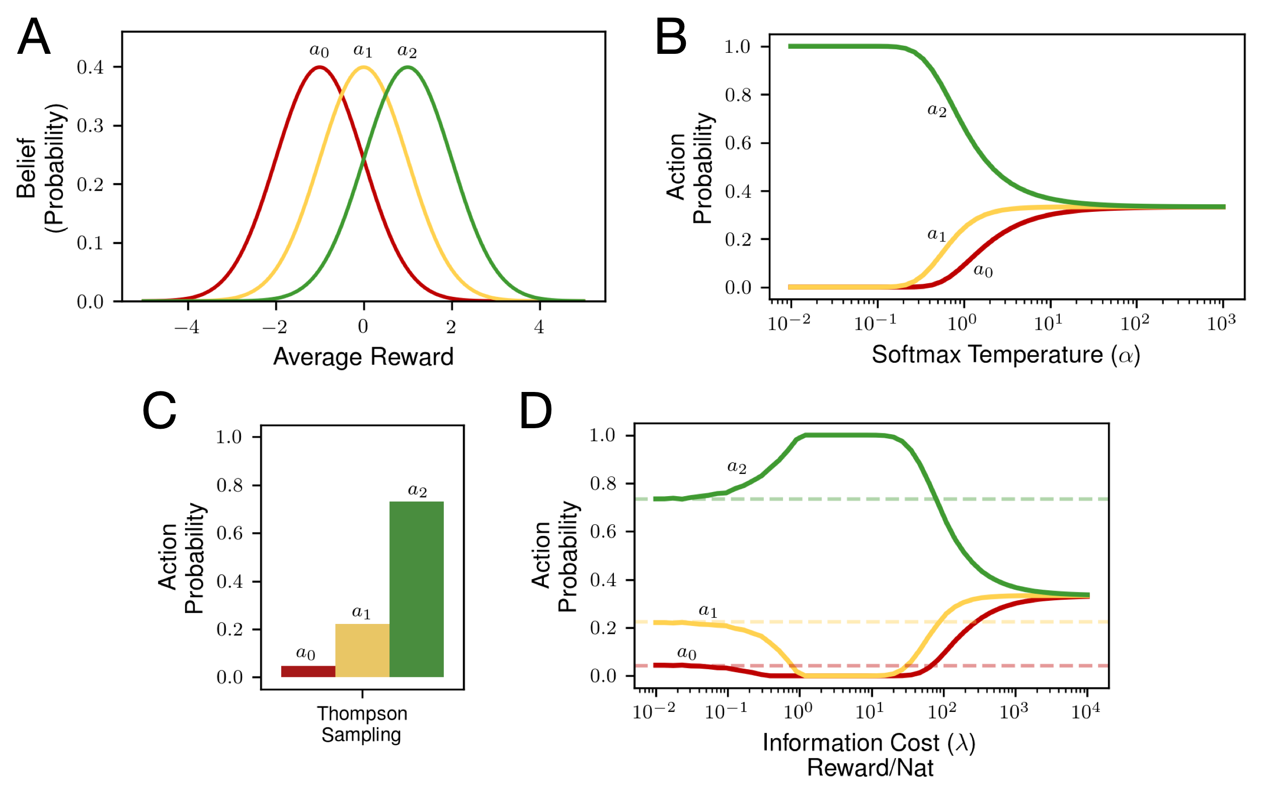
Since BLASTS constructs the estimate-to-action channel that optimally trades off utility and rate, the action distribution it generates is primarily sensitive to the rate parameter, , and the environment-estimator, . To illustrate the behavior of the optimal decision-rule, we conducted two sets of simulations that manipulated these factors in simple three-armed bandit tasks. Our first set of simulations examined the effect of different values of the rate parameter , which intuitively corresponds to the cost of information measured in units of utils per nat. We calculated the marginal action distribution, , where the belief distribution over average rewards for the three arms was represented by three independent Gaussian distributions respectively centered at , , and ; all three distributions had a standard deviation of (Figure 2A).
Remarkably, even on this simple problem, BLASTS displays three qualitatively different regimes of action selection when varying the rate parameter, , from to . When information is inexpensive (), the action distribution mimics the exploratory behavior of Thompson Sampling (consistent with theoretical predictions (Arumugam and Van Roy, 2021a)). As information becomes moderately expensive (), BLASTS focuses channel capacity on the actions with higher expected utility by first reducing its selection of the worst action in expectation () followed by the second-worst/second-best action in expectation (), which results in it purely exploiting the best action in expectation (). Finally, as the util per nat becomes even greater () BLASTS produces actions that are uninformed by its beliefs about the environment. This occurs in a manner that resembles a Boltzmann distribution with increasing temperature, eventually saturating at a uniform distribution over actions. These patterns are visualized in Figure 2B-D, which compare action probabilities for Boltzmann, Thompson Sampling, and BLASTS.
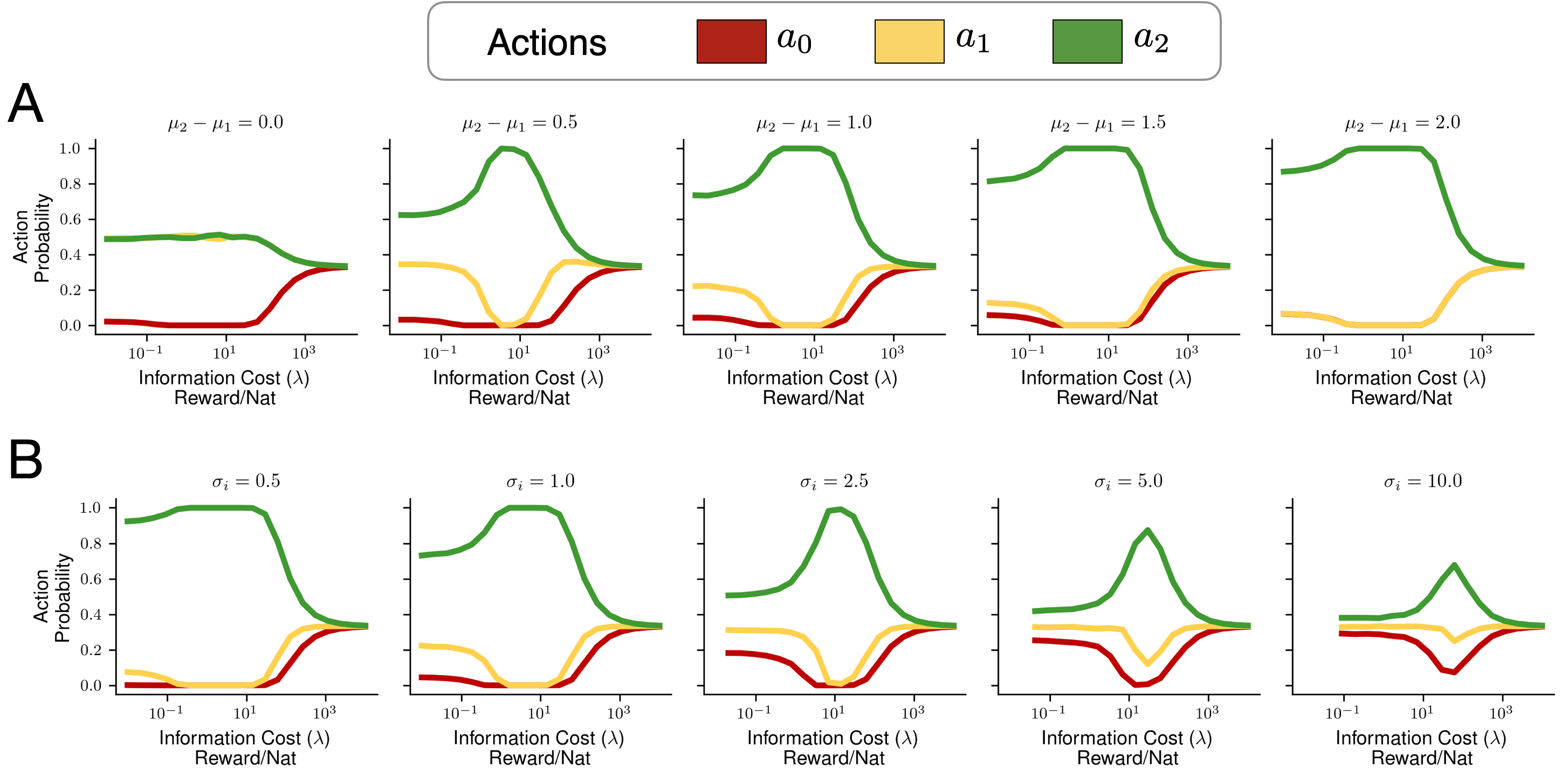
Our second set of simulations examine the relationship between the cost of information and BLASTS action probabilities for different environment-estimates. Specifically, we first examined the effect of changing beliefs about the action gap, the difference between the best and second-best action in expectation (Auer et al., 2002; Agrawal and Goyal, 2012, 2013; Farahmand, 2011; Bellemare et al., 2016). As shown in Figure 3A, when the action gap is lower (corresponding to a more difficult decision-making task), BLASTS chooses the optimal action with lower probability for all values of . In addition, we examined the effect of changing uncertainty in the average rewards by setting different standard deviations for beliefs about the arms. Figure 3B shows that as uncertainty increases, BLASTS is less likely to differentially select an arm even in the “exploitation” regime for moderate values of . Sensitivity to the action gap and uncertainty are key features of BLASTS that derive from the fact that it uses distributional information to guide decision-making, unlike decision-rules such as -greedy or Boltzmann softmax.
2.4 Summary
In the standard formulation of Bayesian decision-making, we assume an environment-estimator and decision-rule that are specified independently. By extending ideas from rate-distortion theory, Arumugam and Van Roy (2021a) defined a notion of capacity-limitations applicable to decision-rules as well as an efficient algorithm for finding an optimal capacity-limited variant of Thompson Sampling (BLASTS). In this section, we analyzed how choice distributions change as a function of the cost of information and current environment estimates, which provides some intuition for how capacity-limitations affect choice from the agent’s subjective point of view. In the next section, we take a more objective point of view by studying the learning dynamics that arise when capacity-limited agents interact with an environment over time.
3 Capacity-Limited Bayesian Reinforcement Learning
The preceding section provides a cursory overview of how rate-distortion theory accommodates capacity-limited learning within a Bayesian decision-making agent. In this section, we aim to provide mathematically-precise instantiations of the earlier concepts for three distinct problem classes: (1) continual or lifelong learning, (2) multi-armed bandits, and (3) episodic Markov decision processes. Of these three types of environments, the capacity-limited learning framework we provide for continual learning is a novel contribution of this work whereas the remaining two classes (which emerge as special cases of continual learning) have been examined in prior work (Arumugam and Van Roy, 2021a, b, 2022).
3.1 Preliminaries
In this section, we provide brief details on our notation and information-theoretic quantities used throughout the remainder of the paper. We encourage readers to consult (Cover and Thomas, 2012; Gray, 2011; Duchi, 2021; Polyanskiy and Wu, 2022) for more background on information theory. We define all random variables with respect to a probability space . For any two random variables and , we use the shorthand notation to denote the law or distribution of the random variable and, analogously, as well as for the associated conditional distributions given and a realization of , respectively. For the ease of exposition, we will assume throughout this work that all random variables are discrete; aside from there being essentially no loss of generality by assuming this (see Equation 2.2.1 of (Duchi, 2021) or Theorem 4.5 of (Polyanskiy and Wu, 2022) for the Gelfand-Yaglom-Perez definition of divergence (Gelfand and Yaglom, 1959; Perez, 1959)), extensions to arbitrary random variables taking values on abstract spaces are straightforward and any theoretical results presented follow through naturally to these settings. In the case of any mentioned real-valued or vector-valued random variables, one should think of these as discrete with support obtained from some suitably fine quantization such that the resulting discretization error is negligible. For any natural number , we denote the index set as . For any arbitrary set , denotes the set of all probability distributions with support on . For any two arbitrary sets and , we denote the class of all functions mapping from to as .
We define the mutual information between any two random variables through the Kullback-Leibler (KL) divergence:
where are both probability distributions. An analogous definition of conditional mutual information holds through the expected KL-divergence for any three random variables :
With these definitions in hand, we may define the entropy and conditional entropy for any two random variables as
This yields the following identities for mutual information and conditional mutual information for any three arbitrary random variables , , and :
Finally, for any three random variables , , and which form the Markov chain , we have the following data-processing inequality: .
In subsequent sections, the random variable will often appear denoting the current history of an agent’s interaction with the environment. We will use as shorthand notation for the conditional distribution of any random variable given a random realization of an agent’s history , at any timestep . Similarly, we denote the entropy and conditional entropy conditioned upon a specific realization of an agent’s history , for some timestep , as and , for two arbitrary random variables and . This notation will also apply analogously to the mutual information as well as the conditional mutual information given an arbitrary third random variable, . A reader should interpret this as recognizing that, while standard information-theoretic quantities average over all associated random variables, an agent attempting to quantify information for the purposes of exploration does so not by averaging over all possible histories that it could potentially experience, but rather by conditioning based on the particular random history that it has currently observed thus far. This dependence on the random realization of history makes all of the aforementioned quantities random variables themselves. The traditional notions of conditional entropy and conditional mutual information given the random variable arise by taking an expectation over histories:
Additionally, we will also adopt a similar notation to express a conditional expectation given the random history :
3.2 Continual Learning
At the most abstract level, we may think of a decision-making agent faced with a continual or lifelong learning setting (Thrun and Schwartz, 1994; Konidaris and Barto, 2006; Wilson et al., 2007; Lazaric and Restelli, 2011; Brunskill and Li, 2013, 2015; Isele et al., 2016; Abel et al., 2018) within a single, stationary environment, which makes no further assumptions about Markovity or episodicity; such a problem formulation aligns with those of Lu et al. (2021); Foster et al. (2021); Dong et al. (2022), spanning multi-armed bandits and reinforcement-learning problems (Lattimore and Szepesvári, 2020; Sutton and Barto, 1998). More concretely, we adopt a generic agent-environment interface where, at each time period , the agent executes an action within an environment that results in an associated next observation . This sequential interaction between agent and environment yields an associated history£££At the very first timestep, the initial history only consists of an initial observation . at each timestep , , representing the action-observation sequence available to the agent upon making its selection of its current action . We may characterize the overall environment as containing the action set , observation set , and observation function , prescribing the distribution over next observations given the current history and action selection: .
An agent’s policy encapsulates the relationship between the history encountered in each timestep and the executed action such that assigns a probability to each action given the history. Preferences across histories are expressed via a known reward function so that an agent enjoys a reward on each timestep. Given any finite time horizon , the accumulation of rewards provide a notion of return . To develop preferences over behaviors and to help facilitate action selection, it is often natural to associate with each policy a corresponding expected return or action-value function across the horizon as where the expectation integrates over the randomness in the policy as well as the observation function . Traditionally, an agent designer focuses on agents that strive to achieve the optimal value within the confines of some policy class , , . The optimal policy then follows by acting greedily with respect to this optimal value function: .
Observe that when rewards and the distribution of the next observation depend only on the current observation-action pair , rather than the full history , we recover the traditional Markov Decision Process (Bellman, 1957; Puterman, 1994) studied throughout the reinforcement-learning literature (Sutton and Barto, 1998). Alternatively, when these quantities rely solely upon the most recent action , we recover the traditional multi-armed bandit (Lai and Robbins, 1985; Bubeck and Cesa-Bianchi, 2012; Lattimore and Szepesvári, 2020). Regardless of precisely which of these two problem settings one encounters, a default presumption throughout both literatures is that an agent should always act in pursuit of learning an optimal policy . Bayesian decision-making agents (Bellman and Kalaba, 1959; Duff, 2002; Ghavamzadeh et al., 2015) aim to achieve this by explicitly representing and maintaining the agent’s current knowledge of the environment, recognizing that it is the uncertainty in the underlying environment that drives uncertainty in optimal behavior . A Bayesian learner reflects this uncertainty through conditional probabilities , aimed at estimating the underlying environment. Under the prior distribution , the entropy of this random variable implies that a total of bits quantify all of the information needed for identifying the environment and, as a result, synthesizing optimal behavior. For sufficiently rich and complex environments, however, can become prohibitively large or even infinite, making the pursuit of an optimal policy entirely intractable.
The core insight of this work is recognizing that a delicate balance between the amount of information processing that goes into a decision (cognitive load) and the quality of that decision (utility) can be aptly characterized through rate-distortion theory, providing a formal framework for capacity-limited decision making. At each time period , the agent’s current knowledge about the underlying environment is fully specified by the distribution . Whereas the standard Thompson Sampling (TS) agent will attempt to use this knowledge for identifying an optimal action by default, a capacity-limited agent may not be capable of operationalizing all bits of information from its beliefs about the world to discern a current action .
Rate-distortion theory (Shannon, 1959; Berger, 1971) is a branch of information theory (Shannon, 1948; Cover and Thomas, 2012) dedicated to the study of lossy compression problems which necessarily must optimize for a balance between the raw amount of information retained in the compression and the utility of those bits for some downstream task; a classic example of this from the information-theory literature is a particular image that must be compressed down to a smaller resolution (fewer bits of information) without overly compromising the visual acuity of the content (bounded distortion). A capacity-limited agent will take its current knowledge as the information source to be compressed in each time period . The lossy compression mechanism or channel itself is simply a conditional probability distribution that maps a potential realization of the unknown environment to a corresponding distribution over actions for the current time period. Naturally, the amount of information used from the environment to identify this action is precisely quantified by the mutual information between these two random variables, , where the subscript capture the dependence of the agent’s beliefs on the current random history .
Aside from identifying the data to be compressed, a lossy compression problem also requires the specification of a distortion function which helps distinguish between useful and irrelevant bits of information contained in the environment. Intuitively, environment-action pairs yielding high distortion are commensurate with achieving high loss and, naturally, a good lossy compression mechanism is one that can avoid large expected distortion, Putting these two pieces together, the fundamental limit of lossy compression is given by the rate-distortion function
| (4) |
where we denote the conditional distribution that achieves this infimum as where is the random variable representing this target action that achieves the rate-distortion limit. A bounded decision maker with limited information processing can only hope to make near-optimal decisions. Thus, a natural way to quantify distortion is given by the expected performance shortfall between an optimal decision and the chosen one.
The distortion threshold input to the rate-distortion function is a free parameter specified by an agent designer that communicates a preferences for the minimization of rate versus the minimization of distortion. This aligns with a perspective that a decision-making agent has a certain degree of tolerance for sub-optimal behavior and, with that degree of error in mind, chooses among the viable near-optimal solutions that incur the least cognitive load to compute actions from beliefs about the world. If one is willing to tolerate significant errors and large amounts of regret, than decision-making should be far simpler in the sense that very few bits of information from beliefs about the environment are needed to select an action. Conversely, as prioritizing near-optimal behavior becomes more important, each decision requires greater cognitive effort as measure by the amount of information utilized to compute actions from current beliefs. The power of rate-distortion theory, in part, lies in the ability to give precise mathematical form to this intuitive narrative, as demonstrated by Fact 1.
Fact 1 (Lemma 10.4.1 (Cover and Thomas, 2012)).
For all and any , the rate-distortion function is a non-negative, convex, and non-increasing function in its argument.
In particular, Fact 1 establishes the following relationship for any ,
confirming that the amount of information used to determine is less than what would be needed to identify an optimal action .
Alternatively, in lieu of presuming that an agent is cognizant of what constitutes a “good enough” solution, one may instead adopt the perspective that an agent is made aware of its capacity limitations. In this context, agent capacity refers to a bound on the number of bits an agent may operationalize from its beliefs about the world in order to discern its current action selection . Conveniently, the information-theoretic optimal solution is characterized by the Shannon distortion-rate function:
| (5) |
Natural limitations on a decision-making agent’s time or computational resources can be translated and expressed as limitations on the sheer amount of information that can possibly be leveraged from beliefs about the environment to execute actions; the distortion-rate function quantifies the fundamental limit on minimum expected distortion that an agent should expect under such a capacity constraint. It is oftentimes convenient that the rate-distortion function and distortion-rate function are inverses of one another such that .
In this section, we have provided a mathematical formulation for how a capacity-limited agent might go about action selections in each time period that limit overall cognitive load in an information-theoretically optimal fashion while also leveraging as much of its environmental knowledge as possible to behave with limited sub-optimality. To elucidate the value of this formulation, we dedicate the following sections to simpler and more tractable problem settings which allow for theoretical and as well as empirical analysis.
3.3 Multi-Armed Bandit
In this section, we begin with the formal specification of a multi-armed bandit problem (Lai and Robbins, 1985; Bubeck and Cesa-Bianchi, 2012; Lattimore and Szepesvári, 2020) before presenting Thompson Sampling as a quintessential algorithm for identifying optimal actions. We then present a corresponding generalization of Thompson Sampling that takes an agent’s capacity limitations into account.
3.3.1 Problem Formulation
We obtain a bandit environment as a special case of the problem formulation given in Section 3.2 by treating the initial observation as null while each subsequent observation denotes a reward signal drawn from an observation function that only depends on the most recent action selection and not the current history . While the actions and total time periods are known to the agent, the underlying reward function is unknown and, consequently, the environment is itself a random variable such that We let denote the mean reward function , , and define an optimal action as achieving the maximal mean reward denoted as , both of which are random variables due to their dependence on .
Observe that, if the agent knew the underlying environment exactly, there would be no uncertainty in the optimal action ; consequently, it is the agent’s epistemic uncertainty (Der Kiureghian and Ditlevsen, 2009) in that drives uncertainty in and, since learning is the process of acquiring information, an agent explores to learn about the environment and reduce this uncertainty. As there is only a null history at the start , initial uncertainty in the environment is given by the prior probabilities while, as time unfolds, updated knowledge of the environment is reflected by posterior probabilities .
For a fixed choice of environment , the performance of an agent is assessed through the regret of its policies over time periods
Since the environment is itself a random quantity, we integrate over this randomness with respect to the prior to arrive at the Bayesian regret:
The customary goal within a multi-armed bandit problem is to identify an optimal action and provably-efficient bandit learning emerges from algorithms whose Bayesian regret can be bounded from above. In the next section, we review one such algorithm that is widely used in practice before motivating consideration of satisficing solutions for bandit problems.
3.3.2 Thompson Sampling & Satisficing
A standard choice of algorithm for addressing multi-armed bandit problems is Thompson Sampling (TS) (Thompson, 1933; Russo et al., 2018), which has been well-studied both theoretically (Auer et al., 2002; Agrawal and Goyal, 2012, 2013; Bubeck and Liu, 2013; Russo and Van Roy, 2016) and empirically (Granmo, 2010; Scott, 2010; Chapelle and Li, 2011; Gopalan et al., 2014). For convenience, we provide generic pseudocode for TS as Algorithm 3, whereas more granular classes of bandit problems (Bernoulli bandits or Gaussian bandits, for example) can often lead to more computationally explicit versions of TS that leverage special structure like conjugate priors (see (Russo et al., 2018) for more detailed implementations). In each time period , a TS agent proceeds by drawing one sample , representing a statistically-plausible hypothesis about the underlying environment based on the agent’s current posterior beliefs from observing the history ; the agent then proceeds as if this sample dictates reality and acts optimally with respect to it, drawing an action to execute this time period uniformly at random among the optimal actions for this realization of of the environment. Executing actions in this manner recovers the hallmark probability-matching principle (Scott, 2010; Russo and Van Roy, 2016) of TS whereby, in each time period , the agent selects actions according to their (posterior) probability of being optimal given everything observed up to this point in or, more formally, , .
Aside from admitting a simple, computationally-efficient procedure for learning optimal actions over time, TS also boasts rigorous theoretical guarantees. While the classic Gittins’ indices (Gittins, 1979; Gittins et al., 2011) yield the Bayes-optimal policy, they are extremely limited to problems of modest size such that, for our finite-horizon setting, they are computationally intractable. Nevertheless, Russo and Van Roy (2016) offer a rigorous corroborating analysis of TS that, for our setting, yields an information-theoretic Bayesian regret bound:
This result communicates that the overall Bayesian regret of TS is governed by the entropy over the optimal arm under the prior . When an agent designer has strong prior knowledge about the optimal arm, initializing TS accordingly results in a very small upper bound on Bayesian regret; conversely, in the case of an uninformative prior, the worst-case entropy over the optimal arm is equal to and the second inequality is tight, which still matches the best-known regret lower bound for multi-armed bandit problems up to logarithmic factors (Bubeck and Liu, 2013).
Naturally, a core premise of this work is to consider decision-making problems where an agent’s inherent and unavoidable capacity limitations drastically impact the tractability of learning optimal actions. While there are other classes of algorithms for handling multi-armed bandit problems (Auer et al., 2002; Ryzhov et al., 2012; Powell and Ryzhov, 2012; Russo and Van Roy, 2014, 2018a), TS serves an exemplary representative among them as it relentlessly pursues the optimal action , by design. Consider a human decision maker faced with a bandit problem containing (one trillion) arms – does one genuinely expect any individual to successfully identify ? Similarly, the final inequality in the Bayesian regret bound above informs us that the performance shortfall of TS will increase as the number of actions tends to , quantifying the folly of pursuing as the agent continuously experiments with untested but potentially optimal actions.
Satisficing is a longstanding, well-studied idea about how to understand resource-limited cognition (Simon, 1955, 1956; Newell et al., 1958; Newell and Simon, 1972; Simon, 1982) in which an agent settles for the first recovered solution that is deemed to be “good enough,” for some suitable notion of goodness. Inspired by this idea, Russo and Van Roy (2018b, 2022) present the Satisficing Thompson Sampling (STS) algorithm, which we present as Algorithm 4, to address the shortcomings of algorithms like TS that relentlessly pursue . STS employs a minimal adjustment to the original TS algorithm through a threshold parameter , which an agent designer may use to communicate that identifying a -optimal action would be sufficient for their needs. The use of a minimum over all such -optimal actions instead of a uniform distribution reflects the idea of settling for the first solution deemed to be “good enough” according to . Naturally, the intuition follows that as increases and the STS agent becomes more permissive, such -optimal actions can be found in potentially far fewer time periods than what is needed to obtain through TS. If we define an analogous random variable to as then STS simply employs probability matching as , and, as , recovers TS as a special case. Russo and Van Roy (2022) go on to prove a complementary information-theoretic regret bound for STS, which depends on , rather than the entropy of , .
While it is clear that STS does embody the principle of satisficing for a capacity-limited decision maker, the action targeted by a STS agent instead of only achieves some arbitrary and unspecified trade-off between the simplicity of what the agent set out to learn and the utility of the resulting solution, as varies. This is in contrast to a resource-rational approach (Anderson, 1990; Griffiths et al., 2015) which aims to instead strike the best trade-off between these two competing interests. One interpretation of the next section is that we provide a mathematically-precise characterization of such resource-rational solutions through rate-distortion theory.
3.3.3 Rate-Distortion Theory for Target Actions
To see how the rate-distortion function (Equation 4) fits into the preceding discussion of Thompson Sampling and STS, Arumugam and Van Roy (2021a) replace the of Equation 4 with a target action . This notion of a target action based on the observation is that is merely a statistic of the environment whose computation is determined by some abstract function . It follows that an alternative surrogate action an agent may prioritize during learning will be some other computable statistic of the environment that embodies a kind of trade-off between two key properties: (1) ease of learnability and (2) bounded sub-optimality or performance shortfall relative to .
The previous section already gives two concrete examples of potential target actions, and , where the former represents an extreme point on the spectrum of potential learning targets as one that demands a potentially intractable amount of information to identify but comes with no sub-optimality. At the other end of the spectrum, there is simply the uniform random action which requires no learning or sampling on the part of the agent to learn it but, in general, will likely lead to considerably large performance shortfall relative to an optimal solution. While, for any fixed , lives in between these extremes, it also suffers from two shortcomings of its own. Firstly, by virtue of satisficing and a willingness to settle for anything that is “good enough,” it is unclear how well balances between the two aforementioned desiderata. In particular, the parameterization of around as an upper bound to the expected regret suggests that there could exist an even simpler target action than that is also -optimal but easier to learn insofar as it requires the agent obtain fewer bits of information from the environment. Secondly, from a computational perspective, a STS agent striving to learn (just as a TS agent does for learning ) computes the same statistic repeatedly across all time periods. Meanwhile, with every step of interaction, the agent’s knowledge of the environment is further refined, potentially changing the outlook on what can be tractably learned in subsequent time periods. This suggests that one stands to have considerable gains by designing agents that adapt their learning target as knowledge of the environment accumulates, rather than iterating on the same static computation.
Recall that from Equation 4, a target action following distribution achieves the rate-distortion limit given by
| (6) |
In order to satisfy the second desideratum of bounded performance shortfall for learning targets and to facilitate a regret analysis, Arumugam and Van Roy (2021a) define the distortion function as
While having bounded expected distortion satisfies our second criterion for a learning target, the fact that requires fewer bits of information to learn is immediately given by properties of the rate-distortion function itself, through Fact 1.
Abstractly, one could consider a procedure like Algorithm 5 that, for an input distortion threshold , identifies the corresponding target action of Equation 6 and then performs probability matching with respect to it. The following theorem provides an information-theoretic Bayesian regret bound that generalizes the performance guarantee of traditional TS by Russo and Van Roy (2016) while also providing a more direct connection to the rate-distortion function than Theorem 3 of Arumugam and Van Roy (2021a) using proof techniques developed by Arumugam and Van Roy (2022).
Theorem 1.
For any ,
When and the agent designer is not willing to tolerate any sub-optimality relative to , Fact 1 allows this bound to recover the guarantee of TS exactly. At the other extreme, increasing to 1 (recall that mean reward are bounded in ) allows and the agent has nothing to learn from the environment but also suffers the linear regret of . Naturally, the “sweet spot” is to entertain intermediate values of where smaller values will lead to larger amounts of information needed to identify the corresponding target action, but not as many bits as what learning necessarily entails.
Just as in the previous subsection, it may often be sensible to also consider a scenario where an agent designer is unable to precisely specify a reasonable threshold on expected distortion and can, instead, only characterize a limit on the amount of information an agent may acquire from the environment . One might interpret this as a notion of capacity which differs quite fundamentally from other notions examined in prior work (Lai and Gershman, 2021; Gershman, 2021) (see Section 4 for a more in-depth comparison). For this, we may consider the distortion-rate function
| (7) |
which quantifies the fundamental limit of lossy compression subject to a rate constraint, rather than the distortion threshold of . Similar to the rate-distortion function, however, the distortion rate function also adheres to the three properties outlined in Fact 1. More importantly, it is the inverse of the rate-distortion function such that for any and . Consequently, by selecting as input to Algorithm 5, we immediately recover the following corollary to Theorem 1 that provides an information-theoretic Bayesian regret bound in terms of agent capacity, rather than a threshold on expected distortion.
Corollary 1.
For any ,
The semantics of this performance guarantee are identical to those of Theorem 1, only now expressed explicitly through the agent’s capacity . Namely, when the agent has no capacity for learning , and the agent incurs linear regret of . Conversely, with sufficient capacity , and we recover the regret bound of Thompson Sampling. Intermediate values of agent capacity will result in an agent that fully utilizes its capacity to acquire no more than bits of information from the environment, resulting in the minimum possible expected distortion quantified by .
While a non-technical reader of this section should remain unencumbered by the mathematical minutia of these theoretical results, the salient takeaway is an affirmation that rate-distortion theory not only provides an intuitive and mathematically-precise articulation of capacity-limited Bayesian decision-making in multi-armed bandits, but also facilitates the design of a complementary algorithm for statistically-efficient learning. The next section proceeds to illustrate how these theoretical results hold up in practice.
3.3.4 Experiments
In order to make the algorithm of the previous section (Algorithm 5) amenable to practical implementation, Arumugam and Van Roy (2021a) look to the classic Blahut-Arimoto algorithm (Blahut, 1972; Arimoto, 1972). Just as TS and STS perform probability matching with respect to and in each time period, respectively, the Blahut-Arimoto STS (BLASTS) algorithm (presented as Algorithm 2 where one should recall that reward maximization and regret minimization are equivalent) conducts probability matching with respect to in each time period to determine the policy: , . For two discrete random variables representing an uncompressed information source and the resulting lossy compression, the Blahut-Arimoto algorithm computes the channel that achieves the rate-distortion limit (that is, achieve the infimum in Equation 6) by iterating alternating update equations until convergence. More concretely, the algorithm is derived by optimizing the Lagrangian of the constrained optimization (Boyd and Vandenberghe, 2004) that is the rate-distortion function, which is itself known to be a convex optimization problem (Chiang and Boyd, 2004). We refer readers to (Arumugam and Van Roy, 2021a) for precise computational details of the Blahut-Arimoto algorithm for solving the rate-distortion function that yields as well as (Arumugam and Van Roy, 2021b) for details on the exact theoretical derivation.
One salient detail that emerges from using the Blahut-Arimoto algorithm in this manner is that it an agent designer’s no longer specifies a distortion threshold as input but, instead, provides a value of the Lagrange multiplier ; lower values of communicate a preferences for rate minimization whereas larger values of prioritize distortion minimization. To each value of , there is an associate distortion threshold as represents the desired slope achieved along the corresponding rate-distortion curve (Blahut, 1972; Csiszár, 1974a, b). As, in practice, tends to be a continuous distribution, Arumugam and Van Roy (2021a) induce a discrete information source by drawing a sufficiently large number of Monte-Carlo samples and leveraging the resulting empirical distribution, which turns out to be a theoretically sound estimator of the true rate-distortion function (Harrison and Kontoyiannis, 2008; Palaiyanur and Sahai, 2008).
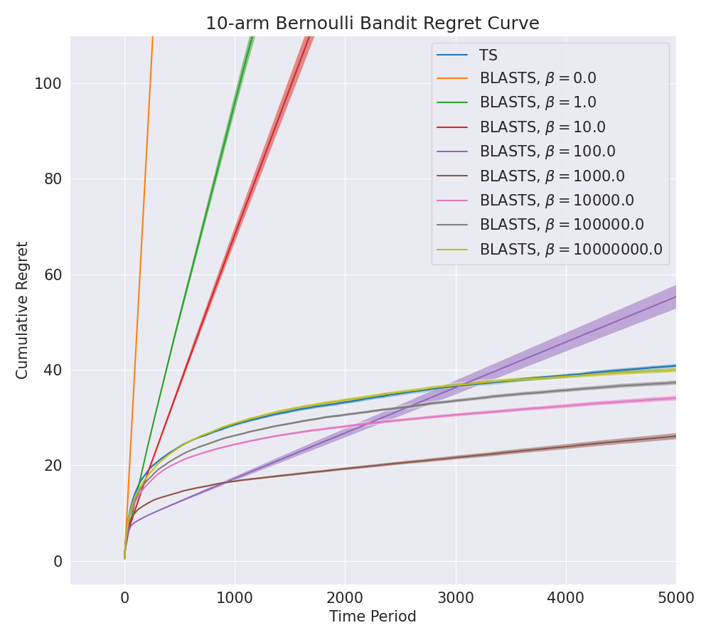
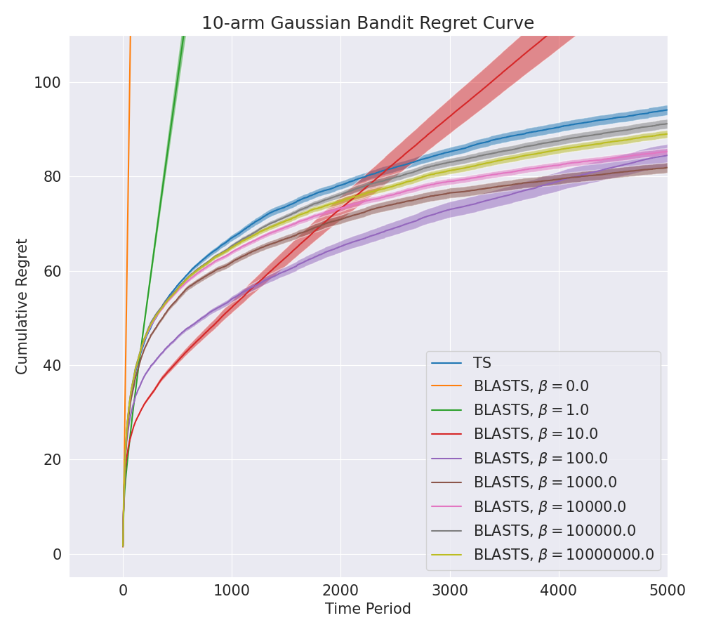
As these target actions are born out of a need to balance the simplicity and utility of what an agent aims to learn from its interactions within the environment, we can decompose empirical results into those that affirm these two criteria are satisfied in isolation. Since assessing utility or, equivalently, performance shortfall is a standard evaluation metric used throughout the literature, we begin there and offer regret curves in Figure 4 for Bernoulli and Gaussian bandits with 10 independent arms (matching, for example, the empirical evaluation of Russo and Van Roy (2018a)); recall that the former implies Bernoulli rewards while the latter yields Gaussian rewards with unit variance . We evaluate TS and BLASTS agents where, for the latter, the Lagrange multiplier hyperparameter is fixed and tested over a broad range of values. All agents begin with a prior for each action of the Bernoulli bandit and a prior for the Gaussian bandit. For each individual agent, the cumulative regret incurred by the agent is plotted over each time period .
Recalling that our distortion function is directly connected to the expected regret of the BLASTS agent, we observe that smaller values of so aggressively prioritize rate minimization that the resulting agents incur linear regret; in both bandit environments, this trend persists for all values . Notably, as , we observe the resulting agents yield performance more similar to regular TS. This observation aligns with expectations since, for a sufficiently large value of , the Blahut-Arimoto algorithm will proceed to return a channel that only places probability mass on the distortion-minimizing actions, which are indeed, the optimal actions for each realization of the environment. A notable auxiliary finding in these results, also seen in the original experiments of Arumugam and Van Roy (2021a), is that intermediate values of manage to yield regret curves converging towards the optimal policy more efficiently that TS; this is, of course, only possible when the distortion threshold implied by a particular setting of falls below the smallest action gap of the bandit problem.
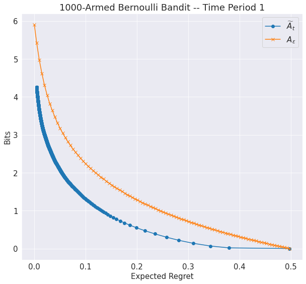
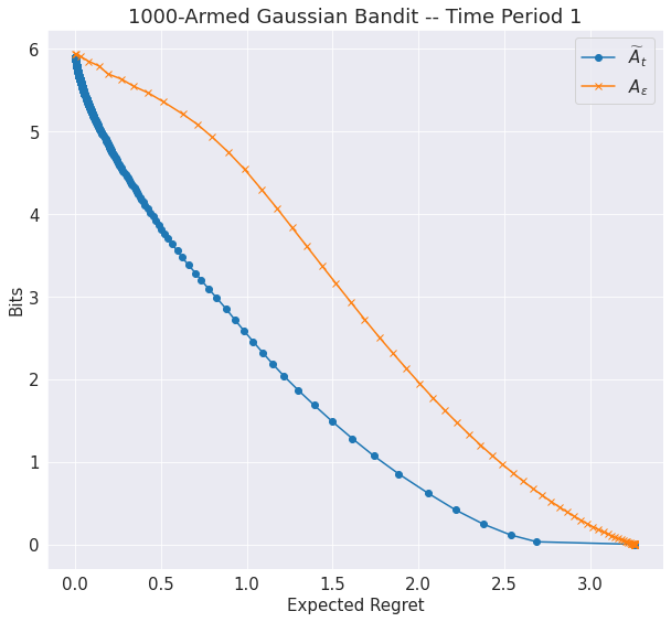
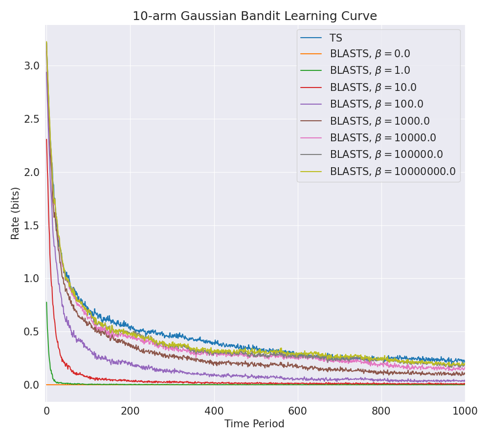
While the previous experiments confirm that BLASTS can be used to instantiate a broad spectrum of agents that target actions of varying utilities, it is difficult to assess the simplicity of these targets and discern whether or not less-performant target actions can in fact be identified more quickly than near-optimal ones. As a starting point, one might begin with the agent’s prior over the environment and compute to quantify how much information each agent’s initial learning target requires from the environment a priori. In Figure 5, we compare this to and sweep over the respective and values to generate the result rate-distortion curves for Bernoulli and Gaussian bandits with 1000 independent arms. The results corroborate earlier discussion of how a STS agent engages with a learning target that yields some trade-off between ease of learnability and performance, but not necessarily the best trade-off. In contrast, since (where the approximation is due to sampling), we expect and do indeed recover a better trade-off between rate and performance using the Blahut-Arimoto algorithm. To verify that target actions at the lower end of the spectrum (lower rate and higher distortion) can indeed by learned more quickly, we can plot the rate of the channel computed by BLASTS across time periods, as shown in Figure 6; for TS, we additionally plot the entropy over the optimal action as time passes and observe that smaller values of lead to learning targets with smaller initial rates that decay much more quickly than their counterparts at larger values of . Again, as , these rate curves concentrate around that of regular TS.
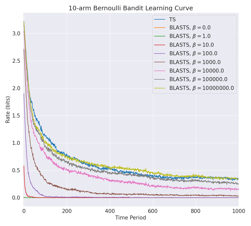
Overall, this section has provided an overview of prior work that moves past the standard goal of finding optimal actions in multi-armed bandit problems and towards capacity-limited decision-making agents. Extending beyond the empirical findings observed in these prior works, we provide additional experiments (see Figure 6) that show how the minimization of rate leads to target actions that are simpler to learn, allowing for an agent to curtail its interactions with the environment in fewer time periods and respect limitations on time and computational resources. Crucially, rate-distortion theory emerges as a natural conduit for identifying target actions that balance between respecting an agent’s limits while still being sufficiently useful for the task at hand. In the next section, we extend this line of thinking to the episodic reinforcement-learning problem and survey recent theoretical results in this space that, analogous to Theorem 1 and Corollary 1, set the stage for subsequent empirical investigations into their practical veracity for both biological and artificial decision-making agents.
3.4 Episodic Reinforcement Learning
In this section, we again specialize the general problem formulation of Section 3.2, this time by introducing the assumption of episodicity commonly made throughout the reinforcement-learning literature. Just as in the preceding section, Thompson Sampling will again reappear as a quintessential algorithm for addressing exploration under an additional assumption that planning across any world model is always computationally feasible. Under this caveat, we survey existing theoretical results which accommodate capacity-limited agents via rate-distortion theory.
3.4.1 Problem Formulation
We formulate a sequential decision-making problem as an episodic, finite-horizon Markov Decision Process (MDP) (Bellman, 1957; Puterman, 1994) defined by . Here denotes a set of states, is a set of actions, is a deterministic reward or utility function providing evaluative feedback signals, is a transition function prescribing distributions over next states, is an initial state distribution, and is the maximum length or horizon. Within each one of episodes, the agent acts for exactly steps beginning with an initial state . For each timestep , the agent observes the current state , selects action , enjoys a reward , and transitions to the next state .
A stationary, stochastic policy for timestep , , encodes behavior as a mapping from states to distributions over actions. Letting denote the class of all stationary, stochastic policies, a non-stationary policy is a collection of exactly stationary, stochastic policies whose overall performance in any MDP at timestep when starting at state and taking action is assessed by its associated action-value function , where the expectation integrates over randomness in the action selections and transition dynamics. Taking the corresponding value function as , we define the optimal policy as achieving supremal value for all , . We let be the random variable denoting the trajectory experienced by the agent in the th episode. Meanwhile, is the random variable representing the entire history of the agent’s interaction within the environment at the start of the th episode.
As is standard in Bayesian reinforcement learning (Bellman and Kalaba, 1959; Duff, 2002; Ghavamzadeh et al., 2015), neither the transition function nor the reward function are known to the agent and, consequently, both are treated as random variables. An agent’s initial uncertainty in the (unknown) true MDP is reflected by a prior distribution . As the agent’s history of interaction within the environment unfolds, updated knowledge of the underlying MDP is reflected by posterior probabilities . Since the regret is a random variable due to our uncertainty in , we integrate over this randomness to arrive at the Bayesian regret over episodes:
Just as in the previous section but with a slight abuse of notation, we will use as shorthand notation for the conditional distribution of any random variable given a random realization of an agent’s history , at any episode . Furthermore, we will denote the entropy and conditional entropy conditioned upon a specific realization of an agent’s history , for some episode , as and , for two arbitrary random variables and . This notation will also apply analogously to mutual information: We reiterate that a reader should interpret this as recognizing that, while standard information-theoretic quantities average over all associated random variables, an agent attempting to quantify information for the purposes of exploration does so not by averaging over all possible histories that it could potentially experience, but rather by conditioning based on the particular random history that it has currently observed thus far. The dependence on the realization of a random history makes a random variable and the usual conditional mutual information arises by integrating over this randomness: Additionally, we will also adopt a similar notation to express a conditional expectation given the random history :
3.4.2 Posterior Sampling for Reinforcement Learning
A natural starting point for addressing the exploration challenge in a principled manner is via Thompson Sampling (Thompson, 1933; Russo et al., 2018). The Posterior Sampling for Reinforcement Learning (PSRL) (Strens, 2000; Osband et al., 2013; Osband and Van Roy, 2014; Abbasi-Yadkori and Szepesvari, 2014; Agrawal and Jia, 2017; Osband and Van Roy, 2017; Lu and Van Roy, 2019) algorithm (given as Algorithm 6) does this by, in each episode , sampling a candidate MDP and executing its optimal policy in the environment ; notably, such posterior sampling guarantees the hallmark probability-matching principle of Thompson Sampling: , . The resulting trajectory leads to a new history and an updated posterior over the true MDP .
Unfortunately, for complex environments, pursuit of the exact MDP may be an entirely infeasible goal, akin to pursuing an optimal action within a multi-armed bandit problem. A MDP representing control of a real-world, physical system, for example, suggests that learning the associated transition function requires the agent internalize laws of physics and motion with near-perfect accuracy. More formally, identifying demands the agent obtain exactly bits of information from the environment which, under an uninformative prior, may either be prohibitively large by far exceeding the agent’s capacity constraints or be simply impractical under time and resource constraints (Lu et al., 2021).
3.4.3 Rate-Distortion Theory for Target MDPs
To remedy the intractabilities imposed by PSRL when an agent must contend with an overwhelmingly-complex environment, we once again turn to rate-distortion theory as a tool for defining an information-theoretic surrogate than an agent may use to prioritize its information acquisition strategy in lieu of . If one were to follow the rate-distortion optimization of Equation 4, this would suggest identifying a channel that directly maps a bounded agent’s beliefs about to a behavior policy for use in the current episode . For the purposes of analysis, Arumugam and Van Roy (2022) instead perform lossy MDP compression with the interpretation that various facets of the true MDP must be discarded by a capacity-limited agent who can only hope identify a simplified world model that strives to retain as many salient details as possible. Implicit to such an approach is an assumption that the act of planning (that is, mapping any MDP to its optimal policy ) can always be done in a computationally-efficient manner irrespective of the agent’s capacity limitations. From a mechanistic perspective, this is likely implausible for both artificial agents in large-scale, high-dimensional environments of interest as well as biological agents (Ho et al., 2022). On the other hand, this construction induces a Markov chain , where denotes the compressed world model; by the data-processing inequality, we have for all that , such that minimizing the rate of the lossy MDP compression must also limit the amount of information that flows from the agent’s beliefs about the world to the executed behavior policy.
For the precise details of this MDP compression, we first require (just as with any lossy compression problem) the specification of an information source to be compressed as well as a distortion function that quantifies the loss of fidelity between uncompressed and compressed values. Akin to the multi-armed bandit setting, we will take the agent’s current beliefs as the information source to be compressed in each episode. Unlike in the bandit setting, however, the choice of distortion function presents an opportunity for the agent designer to be judicious in specifying which aspects of the environment are preserved in the agent’s compressed view of the world.
It is fairly well accepted that human beings do not model all facets of the environment when making decisions (Simon, 1956; Gigerenzer and Goldstein, 1996) and the choice of which details are deemed salient enough to warrant retention in the mind of an agent is precisely governed by the choice of distortion function. In the computational reinforcement-learning literature, this reality has called into question longstanding approaches to model-based reinforcement learning (Sutton, 1991; Sutton and Barto, 1998; Littman, 2015) which use standard maximum-likelihood estimation techniques that endeavor to learn the exact model that governs the underlying MDP. The end result has been a flurry of recent work (Silver et al., 2017; Farahmand et al., 2017; Oh et al., 2017; Asadi et al., 2018; Farahmand, 2018; Grimm et al., 2020; D’Oro et al., 2020; Abachi et al., 2020; Cui et al., 2020; Ayoub et al., 2020; Schrittwieser et al., 2020; Nair et al., 2020; Grimm et al., 2021; Nikishin et al., 2022; Voelcker et al., 2022; Grimm et al., 2022) which eschews the traditional maximum-likelihood objective in favor of various surrogate objectives which restrict the focus of the agent’s modeling towards specific aspects of the environment. As the core goal of endowing a decision-making agent with its own internal model of the world is to facilitate model-based planning (Bertsekas, 1995), central among these recent approaches is the value-equivalence principle (Grimm et al., 2020, 2021, 2022) which provides mathematical clarity on how surrogate models can still enable lossless planning relative to the true model of the environment.
For any arbitrary MDP with model and any stationary, stochastic policy , define the Bellman operator as follows:
The Bellman operator is a foundational tool in dynamic-programming approaches to reinforcement learning (Bertsekas, 1995) and gives rise to the classic Bellman equation: for any MDP and any non-stationary policy , the value functions induced by satisfy for all and with , . For any two MDPs and , Grimm et al. (2020) define a notion of equivalence between them despite their differing models. For any policy class and value function class , and are value equivalent with respect to and if and only if , In words, two different models are deemed value equivalent if they induce identical Bellman updates under any pair of policy and value function from . Grimm et al. (2020) prove that when and , the set of all exactly value-equivalent models is a singleton set containing only the true model of the environment. By recognizing that the ability to plan over all arbitrary behaviors is not necessarily in the agent’s best interest and restricting focus to decreasing subsets of policies and value functions , the space of exactly value-equivalent models is monotonically increasing.
Still, however, exact value equivalence still presumes that an agent has the capacity for planning with complete fidelity to the true environment; more plausibly, an agent may only have the resources to plan in an approximately-value-equivalent manner (Grimm et al., 2022). For brevity, let and denote the classes of all reward functions and transition functions, respectively. Recall that, with all known, the uncertainty in a random MDP is entirely driven by its model such that we may think of the support of as . We define a distortion function on pairs of MDPs for any , as
In words, is the supremal squared Bellman error between MDPs and across all states with respect to the policy class and value function class . With an information source and distortion function defined, Arumugam and Van Roy (2022) employ the following rate-distortion function that articulates the lossy MDP compression a capacity-limited decision agent performs to identify a simplified MDP to pursue instead of :
| (8) |
By definition, the target MDP that achieves this rate-distortion limit will demand that the agent acquire fewer bits of information than what is needed to identify . Once again, by virtue of Fact 1, this claim is guaranteed for all and any : . Crucially, however, the use of the value-equivalence principle in the distortion function ensures that agent capacity is allocated towards preserving the regions of the world model needed to plan over behaviors as defined through . Arumugam and Van Roy (2022) establish an information-theoretic Bayesian regret bound for a posterior-sampling algorithm (given as Algorithm 7) that performs probability matching with respect to in each episode , instead of : , where is an uniform upper bound to the information ratio (Russo and Van Roy, 2016, 2014, 2018a) that emerges as a technical assumption for the analysis; a reader should interpret this as a sort of conversion factor communicating the worst case number of units of squared regret incurred by the agent per bit of information acquired from the environment.
Just as with the BLASTS algorithm for the multi-armed bandit setting, this VSRL algorithm directly couples an agent’s exploratory choices in each episode to the epistemic uncertainty it maintains over the resource-rational learning target which it aspires to learn. The bound communicates that an agent with limited capacity must tolerate a higher distortion threshold and pursue the resulting compressed MDP that bears less fidelity to the original MDP; in exchange, the resulting number of bits needed from the environment to identify such a simplified model of the world is given as and guaranteed to be less than the entropy of . Additionally, just as with the regret bound for BLASTS, one can express a near-identical result through the associated distortion-rate function. In particular, this encourages a particular notion of agent capacity as a limit on the number of bits an agent may obtain from its interactions with the environment. Subject to this constraint, the fundamental limit on the amount of expected distortion incurred is given by
| (9) |
Embracing this distortion-rate function and taking the VSRL distortion threshold as allows for a performance guarantee that explicitly accounts for the agent capacity limits:
In summary, under a technical assumption of episodicity for the purposes of analysis, the theoretical results surveyed in this section parallel those of the preceding section for multi-armed bandits. While computational experiments for this episodic reinforcement learning setting have not yet been established due to the computational efficiency of running the Blahut-Arimoto algorithm for such a lossy MDP compression problem, the core takeaway of this section is that there is strong theoretical justification for using these tools from rate-distortion theory to empirically study capacity-limited sequential decision-making agents.
4 Discussion
In this paper, we have introduced capacity-limited Bayesian reinforcement learning, capturing a novel perspective on lifelong learning under a limited cognitive load while also surveying existing theoretical and algorithmic advances specific to multi-armed bandits (Arumugam and Van Roy, 2021a) and reinforcement learning (Arumugam and Van Roy, 2022). Taking a step back, we now situate our contributions in a broader context by reviewing related work on capacity-limited cognition as well as information-theoretic reinforcement learning. As our framework sits at the intersection of Bayesian inference, reinforcement learning, and rate-distortion theory, we use this opportunity to highlight particularly salient pieces of prior work that sit at the intersection Bayesian inference and rate-distortion theory as well as the intersection of reinforcement learning and rate-distortion theory, respectively. Furthermore, while the algorithms discussed in this work all operationalize the Blahut-Arimoto algorithm and Thompson Sampling as the primary mechanisms for handling rate-distortion optimization and exploration respectively, we also discuss opportunities to expand to more sophisticated strategies for computing target actions and exploring once a target action has been determined. Lastly, we conclude our discussion by returning to a key assumption used throughout this work that an agent consistently maintains idealized beliefs about the environment through perfect Bayesian inference.
4.1 Related Work on Learning, Decision-Making, and Rate-Distortion Theory
There is a long, rich literature exploring the natural limitations on time, knowledge, and cognitive capacity faced by human (and animal) decision makers (Simon, 1956; Newell et al., 1958; Newell and Simon, 1972; Shugan, 1980; Simon, 1982; Gigerenzer and Goldstein, 1996; Vul et al., 2014; Griffiths et al., 2015; Gershman et al., 2015; Icard and Goodman, 2015; Lieder and Griffiths, 2020; Amir et al., 2020; Bhui et al., 2021; Brown et al., 2022; Ho et al., 2022; Prystawski et al., 2022; Binz and Schulz, 2022). Crucially, our focus is on a recurring theme throughout this literature of modeling these limitations on cognitive capabilities as being information-theoretic in nature (Sims, 2003; Peng, 2005; Parush et al., 2011; Botvinick et al., 2015; Sims, 2016, 2018; Zenon et al., 2019; Ho et al., 2020; Gershman and Lai, 2020; Gershman, 2020; Mikhael et al., 2021; Lai and Gershman, 2021; Gershman, 2021; Jakob and Gershman, 2022; Bari and Gershman, 2022).
Broadly speaking and under the episodic reinforcement learning formulation of the previous section, these approaches all center around the perspective that a policy should be modeled as a communication channel that, like a human decision-maker with limited information processing capability, is subject to a constraint on the maximal number of bits that may be sent across it. Consequently, an agent aspiring to maximize returns must do so subject to this constraint on policy complexity; conversely, an agent ought to transmit the minimum amount of information possible while it endeavors to reach a desired level of performance (Polani, 2009, 2011; Tishby and Polani, 2011; Rubin et al., 2012). Paralleling the distortion-rate function , the resulting policy-optimization objective follows as It is important to acknowledge that such a formulation sits directly at the intersection of reinforcement learning and rate-distortion theory without invoking any principles of Bayesian inference. Depending on the precise work, subtle variations on this optimization problem exist from choosing a fixed state distribution for the random variable (Polani, 2009, 2011), incorporating the state visitation distribution of the policy being optimized (Still and Precup, 2012; Gershman, 2020; Lai and Gershman, 2021), or assuming access to the generative model of the MDP and decomposing the objective across a finite state space (Tishby and Polani, 2011; Rubin et al., 2012). In all of these cases, the end empirical result tends to converge by also making use of variations on the classic Blahut-Arimoto algorithm to solve the Lagrangian associated with the constrained optimization (Boyd and Vandenberghe, 2004) and produce policies that exhibit higher entropy across states under an excessively limited rate , with a gradual convergence towards the greedy optimal policy as increases.
The alignment between this optimization problem and that of the distortion-rate function is slightly wrinkled by the non-stationarity of the distortion function (here, is used as an analogue to distortion which changes as the policy or channel does) and, when using the policy visitation distribution for , the non-stationarity of the information source. Despite these slight, subtle mismatches with the core rate-distortion problem, the natural synergy between cognitive and computational decision making (Tenenbaum et al., 2011; Lake et al., 2017) has led to various reinforcement-learning approaches that draw direct inspiration from this line of thinking (Klyubin et al., 2005; Ortega and Braun, 2011; Still and Precup, 2012; Ortega and Braun, 2013; Shafieepoorfard et al., 2016; Tiomkin and Tishby, 2017; Goyal et al., 2018; Lerch and Sims, 2018, 2019; Abel et al., 2019; Goyal et al., 2020a, b), most notably including parallel connections to work on “control as inference” or KL-regularized reinforcement learning (Todorov, 2007; Toussaint, 2009; Kappen et al., 2012; Levine, 2018; Ziebart, 2010; Fox et al., 2016; Haarnoja et al., 2017, 2018; Galashov et al., 2019; Tirumala et al., 2019). Nevertheless, despite their empirical successes, such approaches lack principled mechanisms for addressing the exploration challenge (O’Donoghue et al., 2020). In short, the key reason behind this is that the incorporation of Bayesian inference allows for a separation of reducible or epistemic uncertainty that exists due to an agent’s lack of knowledge versus irreducible or aleatoric uncertainty that exists due to the natural stochasticity that may exist within a random outcome (Der Kiureghian and Ditlevsen, 2009). Without leveraging a Bayesian setting, a random variable denoting an agent’s belief about the environment or underlying MDP no longer exists and a channel like the ones explored throughout this work from beliefs to action cease to exist. That said, the notion of rate preserved by these methods has been shown to constitute a reasonable notion of policy complexity (Lai and Gershman, 2021) and future work may benefit from combining the two approaches.
Similar to human decision making (Gershman, 2018; Schulz and Gershman, 2019; Gershman, 2019), provably-efficient reinforcement-learning algorithms have historically relied upon one of two possible exploration strategies: optimism in the face of uncertainty (Kearns and Singh, 2002; Brafman and Tennenholtz, 2002; Kakade, 2003; Auer et al., 2009; Bartlett and Tewari, 2009; Strehl et al., 2009; Jaksch et al., 2010; Dann and Brunskill, 2015; Azar et al., 2017; Dann et al., 2017; Jin et al., 2018; Zanette and Brunskill, 2019; Dong et al., 2022) or posterior sampling (Osband et al., 2013; Osband and Van Roy, 2017; Agrawal and Jia, 2017; Lu and Van Roy, 2019; Lu et al., 2021). While both paradigms have laid down solid theoretical foundations, a line of work has demonstrated how posterior-sampling methods can be more favorable both in theory and in practice (Osband et al., 2013, 2016a, 2016b; Osband and Van Roy, 2017; Osband et al., 2019; Dwaracherla et al., 2020). The theoretical results discussed in this work advance and further generalize this line of thinking through the concept of learning targets (referred to in this work as target actions for clarity of exposition), introduced by Lu et al. (2021), which opens up new avenues for entertaining solutions beyond optimal policies and conditioning an agent’s exploration based on what it endeavors to learn from its environment, not unlike preschool children (Cook et al., 2011). While this literature traditionally centers on consideration of a single agent interacting within its environment, generalizations to multiple agents acting concurrently while coupled through shared beliefs have been formalized and examined in theory as well as in practice (Dimakopoulou and Van Roy, 2018; Dimakopoulou et al., 2018; Chen et al., 2022); translating the ideas discussed here to further account for capacity limitations in that setting constitutes a promising direction for future work.
Finally, we note while the work cited thus far was developed in the reinforcement learning community, the coupling of rate-distortion theory and Bayesian inference to strike a balance between the simplicity and utility of what an agent learns has been studied extensively by Gottwald and Braun (2019), who come from an information-theoretic background studying bounded rationality (Ortega and Braun, 2011, 2013). Perhaps the key distinction between the work surveyed here and theirs is the further incorporation of reinforcement learning, which then provides a slightly more precise foundation upon which existing machinery can be repurposed to derive theoretical results like regret bounds. In contrast, the formulation of Gottwald and Braun (2019) follows more abstract utility-theoretic decision making while also leveraging ideas from microeconomics and generalized beyond from standard Shannon information-theoretic quantities; we refer readers to their excellent, rigorous treatment of this topic.
4.2 Generalizations to Other Families of Decision Rules
The previous sections demonstrated several concrete implementations of capacity-limited Bayesian decision-making. We focused on BLASTS, an algorithm that generalizes Thompson Sampling, which itself is already a quintessential algorithm for navigating the explore-exploit tradeoff in a principled manner in multi-armed bandit and sequential decision-making problems. That said, however, we emphasize that BLASTS is only one particular instantiation of the framework espoused by the rate-distortion function of Equation 4. Here, we briefly sketch other directions in which the framework has been or could be applied.
First, the general framework of capacity-limited Bayesian decision-making can, in principle, be applied to any algorithm that, when supplied with beliefs about the environment and a particular target for learning, induces a policy to execute in the environment. For example, in information-directed sampling, choices are made not only based on current beliefs about immediate rewards but also based on how actions produce informative consequences that can guide future behavior (Russo and Van Roy, 2014, 2018a; Lu et al., 2021; Hao et al., 2022; Hao and Lattimore, 2022). This strategy motivates a decision-maker to engage in direct exploration as opposed to random exploration (Thompson Sampling being one example) (Wilson et al., 2014) and better resolve the explore-exploit dilemma. Work by Arumugam and Van Roy (2021b) has extended the BLASTS algorithm to develop variants of information-directed sampling that similarly minimize the rate between environment estimates and actions. Future work could explore even richer families of decision-rules such as those based on Bayes-optimal solutions over longer time horizons (Duff, 2002) and even ones that look past the KL-divergence as the core quantifier of information (Lattimore and Szepesvári, 2019; Zimmert and Lattimore, 2019; Lattimore and Gyorgy, 2021).
Additionally, BLASTS itself uses a seminal algorithm from the information-theory literature to ultimately address the rate-distortion optimization problem and find the decision-rule that optimally trades off reward and information—namely, the Blahut-Arimoto algorithm (Blahut, 1972; Arimoto, 1972). However, this standard algorithm, while mathematically sound for random variables taking values on abstract spaces (Csiszár, 1974b), can only be made computationally tractable in the face of discrete random variables. Extending to general input distributions (e.g., distributions with continuous or countable support) occurs through the use of an estimator with elegant theoretical properties such as asymptotic consistency (Harrison and Kontoyiannis, 2008; Palaiyanur and Sahai, 2008). Despite this, it is still limited to output distributions that have finite support. This limits its applicability to problems where the action space is finite and relatively small (even if the environment space is complex). Thus, an important direction for future research will be to develop algorithms for finding capacity-limited decision-rules based on versions of Blahut-Arimoto designed for general output distributions (e.g., particle filter-based algorithms (Dauwels, 2005)).
4.3 Capacity-Limited Estimation and Alternative Information Bottlenecks
Throughout this paper, we have assumed that environment estimation is not directly subject to capacity-limitations and that decision-makers perform perfect Bayesian inference. Naturally, however, this idealized scenario isn’t guaranteed to hold for biological or artificial decision making agents. One high-level perspective on the core agent design problem addressed in this work is that decision-making agents cannot acquire unbounded quantities of information from the environment – this reality motivates the need to prioritize information and rate-distortion theory emerges as a natural tool for facilitating such a prioritization scheme.
By the same token, capacity-limited decision-making agents should also seldom find themselves capable of retaining all bits of information uncovered about the underlying environment . If this were possible, then maintaining perfect belief estimates about the environment via would be a reasonable supposition. In reality, however, an agent must also be judicious in what pieces of environment information are actually retained. Lu et al. (2021) introduce terminology for discussing this limited corpus of world knowledge as an environment proxy, . The lack of fidelity between this surrogate and true environment translates to the approximate nature of an agent’s Bayesian inference when maintaining beliefs about in lieu of . For biological decision-making agents, the concept of a proxy seems intuitive as “we are not interested in describing some physically objective world in its totality, but only those aspects of the totality that have relevance as the ‘life space’ of the organism considered. Hence, what we call the ‘environment’ will depend upon the ‘needs,’ ‘drives,’ or ‘goals’ of the organism,” as noted by Herbert Simon many decades ago (Simon, 1956).
Curiously, the relationship between the original environment and this proxy can also be seen as a lossy compression problem where only a salient subset of the cumulative environment information need by retained by the agent for competent decision-making. Consequently, the associated rate-distortion function and the question of what suitable candidate notions of distortion apply may likely be an interesting object of study for future work. Practical optimization of such a rate-distortion function would likely benefit from recent statistical advances in empirical distribution compression (Dwivedi and Mackey, 2022) to get away with representing the information source via a limited number of Monte-Carlo samples.
Finally, although consideration of capacity-limits on inference would extend the scope of the current framework, it is worth noting that recent findings in neuroscience support the possibility of a bottleneck on choice processes even if the bottleneck on inference is minimal. For example, when trained on stimuli presented at different angles, mice have been shown to discriminate orientations as low as - based on behavioral measures (Abdolrahmani et al., 2019). However, direct neural measurements from visual processing regions reveal sensitivity to orientations as low as (Stringer et al., 2021). The higher precision (nearly higher) of sensory versus behavioral discrimination is consistent with a greater information bandwidth on inference compared to choice, as assumed in the current version of the model. Similarly, work tracking the development of decision-making strategies in children provides evidence of capacity limits on choice processes even in the absence of limits on inference. For example, Decker et al. (2016) report that on a task designed to dissociate model-free versus model-based learning mechanisms, 8-12 year olds show signs of encoding changes in transition structure (longer reaction times) but do not appear to use this information to make better decisions, unlike 13-17 year olds and adults. This result is consistent with a distinct bottleneck between inference and action that may have a developmental trajectory. In short, the analyses developed in this paper may shed light on the general computational principles that underlie cases in which decision-makers display optimal inference but suboptimal choice.
4.4 Conclusion
Our goal in this paper has been to review key insights from work on capacity-limited Bayesian decision-making by Arumugam and Van Roy (2021a, 2022) and situate it within existing work on resource-rational cognition and decision-making (Griffiths et al., 2015; Lieder and Griffiths, 2020; Gershman et al., 2015). This discussion naturally leads to a number of questions, in particular, how the general framework presented can be applied to a wider range of algorithms, how other kinds of information bottlenecks could affect learning, and whether humans and other animals are capacity-limited Bayesian decision-makers. We hope that by formally outlining the different components of capacity-limited inference and choice, the current work can facilitate future cross-disciplinary investigations to address such topics.
References
- Abachi et al. [2020] Romina Abachi, Mohammad Ghavamzadeh, and Amir-massoud Farahmand. Policy-aware model learning for policy gradient methods. ArXiv preprint arXiv:2003.00030, 2020.
- Abbasi-Yadkori and Szepesvari [2014] Yasin Abbasi-Yadkori and Csaba Szepesvari. Bayesian optimal control of smoothly parameterized systems: The lazy posterior sampling algorithm. ArXiv preprint arXiv:1406.3926, 2014.
- Abdolrahmani et al. [2019] Mohammad Abdolrahmani, Dmitry R Lyamzin, Ryo Aoki, and Andrea Benucci. Cognitive modulation of interacting corollary discharges in the visual cortex. bioRxiv, page 615229, 2019.
- Abel et al. [2018] David Abel, Yuu Jinnai, Sophie Yue Guo, George Konidaris, and Michael Littman. Policy and value transfer in lifelong reinforcement learning. In International Conference on Machine Learning, pages 20–29. PMLR, 2018.
- Abel et al. [2019] David Abel, Dilip Arumugam, Kavosh Asadi, Yuu Jinnai, Michael L Littman, and Lawson LS Wong. State abstraction as compression in apprenticeship learning. In Proceedings of the AAAI Conference on Artificial Intelligence, volume 33, pages 3134–3142, 2019.
- Agrawal and Goyal [2012] Shipra Agrawal and Navin Goyal. Analysis of Thompson sampling for the multi-armed bandit problem. In Conference on Learning Theory, pages 39–1, 2012.
- Agrawal and Goyal [2013] Shipra Agrawal and Navin Goyal. Further optimal regret bounds for Thompson sampling. In Artificial Intelligence and Statistics, pages 99–107, 2013.
- Agrawal and Jia [2017] Shipra Agrawal and Randy Jia. Optimistic posterior sampling for reinforcement learning: Worst-case regret bounds. In Advances in Neural Information Processing Systems, pages 1184–1194, 2017.
- Amir et al. [2020] Nadav Amir, Reut Suliman-Lavie, Maayan Tal, Sagiv Shifman, Naftali Tishby, and Israel Nelken. Value-complexity tradeoff explains mouse navigational learning. PLOS Computational Biology, 16(12):e1008497, 2020.
- Anderson [1990] John R Anderson. The Adaptive Character of Thought. Lawrence Erlbaum Associates, Inc, 1990.
- Arimoto [1972] Suguru Arimoto. An algorithm for computing the capacity of arbitrary discrete memoryless channels. IEEE Transactions on Information Theory, 18(1):14–20, 1972.
- Arumugam and Van Roy [2021a] Dilip Arumugam and Benjamin Van Roy. Deciding What to Learn: A Rate-Distortion Approach. In International Conference on Machine Learning, pages 373–382. PMLR, 2021a.
- Arumugam and Van Roy [2021b] Dilip Arumugam and Benjamin Van Roy. The Value of Information When Deciding What to Learn. Advances in Neural Information Processing Systems, 34:9816–9827, 2021b.
- Arumugam and Van Roy [2022] Dilip Arumugam and Benjamin Van Roy. Deciding What to Model: Value-Equivalent Sampling for Reinforcement Learning. In Advances in Neural Information Processing Systems, volume 35, 2022.
- Asadi and Littman [2017] Kavosh Asadi and Michael L Littman. An Alternative Softmax Operator for Reinforcement Learning. In International Conference on Machine Learning, pages 243–252. PMLR, 2017.
- Asadi et al. [2018] Kavosh Asadi, Dipendra Misra, and Michael Littman. Lipschitz continuity in model-based reinforcement learning. In International Conference on Machine Learning, pages 264–273. PMLR, 2018.
- Auer [2002] Peter Auer. Using confidence bounds for exploitation-exploration trade-offs. Journal of Machine Learning Research, 3(Nov):397–422, 2002.
- Auer et al. [2002] Peter Auer, Nicolo Cesa-Bianchi, and Paul Fischer. Finite-time Analysis of the Multiarmed Bandit Problem. Machine Learning, 47:235–256, 2002.
- Auer et al. [2009] Peter Auer, Thomas Jaksch, and Ronald Ortner. Near-optimal regret bounds for reinforcement learning. In Advances in Neural Information Processing Systems, pages 89–96, 2009.
- Ayoub et al. [2020] Alex Ayoub, Zeyu Jia, Csaba Szepesvari, Mengdi Wang, and Lin Yang. Model-based reinforcement learning with value-targeted regression. In International Conference on Machine Learning, pages 463–474. PMLR, 2020.
- Azar et al. [2017] Mohammad Gheshlaghi Azar, Ian Osband, and Rémi Munos. Minimax regret bounds for reinforcement learning. In International Conference on Machine Learning, pages 263–272. PMLR, 2017.
- Baker et al. [2009] Chris L Baker, Rebecca Saxe, and Joshua B Tenenbaum. Action understanding as inverse planning. Cognition, 113(3):329–349, 2009.
- Bari and Gershman [2022] Bilal A Bari and Samuel J Gershman. Undermatching is a consequence of policy compression. BioRxiv, 2022.
- Bartlett and Tewari [2009] Peter L Bartlett and Ambuj Tewari. REGAL: A regularization based algorithm for reinforcement learning in weakly communicating MDPs. In Proceedings of the Twenty-Fifth Conference on Uncertainty in Artificial Intelligence, pages 35–42, 2009.
- Battaglia et al. [2013] Peter W Battaglia, Jessica B Hamrick, and Joshua B Tenenbaum. Simulation as an engine of physical scene understanding. Proceedings of the National Academy of Sciences, 110(45):18327–18332, 2013.
- Bellemare et al. [2016] Marc G Bellemare, Georg Ostrovski, Arthur Guez, Philip Thomas, and Rémi Munos. Increasing the action gap: New operators for reinforcement learning. In Proceedings of the AAAI Conference on Artificial Intelligence, volume 30, 2016.
- Bellman [1957] Richard Bellman. A Markovian Decision Process. Journal of Mathematics and Mechanics, pages 679–684, 1957.
- Bellman and Kalaba [1959] Richard Bellman and Robert Kalaba. On Adaptive Control Processes. IRE Transactions on Automatic Control, 4(2):1–9, 1959.
- Berger [1971] Toby Berger. Rate Distortion Theory: A Mathematical Basis for Data Compression. Prentice-Hall, 1971.
- Bertsekas [1995] Dimitri P. Bertsekas. Dynamic Programming and Optimal Control. Athena Scientific, 1995.
- Bhui et al. [2021] Rahul Bhui, Lucy Lai, and Samuel J Gershman. Resource-rational decision making. Current Opinion in Behavioral Sciences, 41:15–21, 2021.
- Binz and Schulz [2022] Marcel Binz and Eric Schulz. Modeling Human Exploration Through Resource-Rational Reinforcement Learning. In Advances in Neural Information Processing Systems, 2022.
- Blahut [1972] Richard Blahut. Computation of channel capacity and rate-distortion functions. IEEE Transactions on Information Theory, 18(4):460–473, 1972.
- Botvinick et al. [2015] Matthew Botvinick, Ari Weinstein, Alec Solway, and Andrew Barto. Reinforcement learning, efficient coding, and the statistics of natural tasks. Current Opinion in Behavioral Sciences, 5:71–77, 2015.
- Boyd and Vandenberghe [2004] Stephen P. Boyd and Lieven Vandenberghe. Convex Optimization. Cambridge University Press, 2004.
- Brafman and Tennenholtz [2002] Ronen I Brafman and Moshe Tennenholtz. R-MAX - A general polynomial time algorithm for near-optimal reinforcement learning. Journal of Machine Learning Research, 3(Oct):213–231, 2002.
- Brown et al. [2022] Vanessa M Brown, Michael N Hallquist, Michael J Frank, and Alexandre Y Dombrovski. Humans adaptively resolve the explore-exploit dilemma under cognitive constraints: Evidence from a multi-armed bandit task. Cognition, 229:105233, 2022.
- Brunskill and Li [2013] Emma Brunskill and Lihong Li. Sample Complexity of Multi-Task Reinforcement Learning. In Proceedings of the Twenty-Ninth Conference on Uncertainty in Artificial Intelligence, pages 122–131, 2013.
- Brunskill and Li [2015] Emma Brunskill and Lihong Li. The online coupon-collector problem and its application to lifelong reinforcement learning. ArXiv preprint arXiv:1506.03379, 2015.
- Bubeck and Cesa-Bianchi [2012] Sébastien Bubeck and Nicolò Cesa-Bianchi. Regret Analysis of Stochastic and Nonstochastic Multi-armed Bandit Problems. Foundations and Trends® in Machine Learning, 5(1):1–122, 2012.
- Bubeck and Liu [2013] Sébastien Bubeck and Che-Yu Liu. Prior-free and prior-dependent regret bounds for Thompson sampling. Advances in Neural Information Processing Systems, 26, 2013.
- Callaway et al. [2022] Frederick Callaway, Bas van Opheusden, Sayan Gul, Priyam Das, Paul M Krueger, Thomas L Griffiths, and Falk Lieder. Rational use of cognitive resources in human planning. Nature Human Behaviour, 6(8):1112–1125, 2022.
- Cesa-Bianchi and Fischer [1998] Nicolo Cesa-Bianchi and Paul Fischer. Finite-Time Regret Bounds for the Multiarmed Bandit Problem. In ICML, volume 98, pages 100–108. Citeseer, 1998.
- Chapelle and Li [2011] Olivier Chapelle and Lihong Li. An empirical evaluation of Thompson sampling. In Advances in Neural Information Processing Systems, pages 2249–2257, 2011.
- Chen et al. [2022] Yan Chen, Perry Dong, Qinxun Bai, Maria Dimakopoulou, Wei Xu, and Zhengyuan Zhou. Society of Agents: Regrets Bounds of Concurrent Thompson Sampling. In Alice H. Oh, Alekh Agarwal, Danielle Belgrave, and Kyunghyun Cho, editors, Advances in Neural Information Processing Systems, 2022.
- Chiang and Boyd [2004] Mung Chiang and Stephen Boyd. Geometric programming duals of channel capacity and rate distortion. IEEE Transactions on Information Theory, 50(2):245–258, 2004.
- Collins and Frank [2013] Anne GE Collins and Michael J Frank. Cognitive control over learning: Creating, clustering, and generalizing task-set structure. Psychological review, 120(1):190, 2013.
- Cook et al. [2011] Claire Cook, Noah D Goodman, and Laura E Schulz. Where science starts: Spontaneous experiments in preschoolers’ exploratory play. Cognition, 120(3):341–349, 2011.
- Cover and Thomas [2012] Thomas M Cover and Joy A Thomas. Elements of Information Theory. John Wiley & Sons, 2012.
- Csiszár [1974a] Imre Csiszár. On the computation of rate-distortion functions (corresp.). IEEE Transactions on Information Theory, 20(1):122–124, 1974a.
- Csiszár [1974b] Imre Csiszár. On an extremum problem of information theory. Studia Scientiarum Mathematicarum Hungarica, 9, 1974b.
- Cui et al. [2020] Brandon Cui, Yinlam Chow, and Mohammad Ghavamzadeh. Control-aware representations for model-based reinforcement learning. In International Conference on Learning Representations, 2020.
- Dann and Brunskill [2015] Christoph Dann and Emma Brunskill. Sample complexity of episodic fixed-horizon reinforcement learning. In Proceedings of the 28th International Conference on Neural Information Processing Systems-Volume 2, pages 2818–2826, 2015.
- Dann et al. [2017] Christoph Dann, Tor Lattimore, and Emma Brunskill. Unifying PAC and regret: Uniform PAC bounds for episodic reinforcement learning. In Proceedings of the 31st International Conference on Neural Information Processing Systems, pages 5717–5727, 2017.
- Dauwels [2005] Justin Dauwels. Numerical computation of the capacity of continuous memoryless channels. In Proceedings of the 26th Symposium on Information Theory in the BENELUX, pages 221–228. Citeseer, 2005.
- Daw et al. [2012] Nathaniel D Daw, Samuel J Gershman, Ben Seymour, Peter Dayan, and J Raymond. Model-based influences on humans’ choices and striatal prediction errors. Neuron, 69(6):1204–1215, 2012. ISSN 2041-1723.
- Dayan and Niv [2008] Peter Dayan and Yael Niv. Reinforcement learning: The good, the bad and the ugly. Current Opinion in Neurobiology, 18(2):185–196, 2008.
- Decker et al. [2016] Johannes H Decker, A Ross Otto, Nathaniel D Daw, and Catherine A Hartley. From creatures of habit to goal-directed learners: Tracking the developmental emergence of model-based reinforcement learning. Psychological Science, 27(6):848–858, 2016.
- Der Kiureghian and Ditlevsen [2009] Armen Der Kiureghian and Ove Ditlevsen. Aleatory or epistemic? Does it matter? Structural Safety, 31(2):105–112, 2009.
- Dimakopoulou and Van Roy [2018] Maria Dimakopoulou and Benjamin Van Roy. Coordinated exploration in concurrent reinforcement learning. In International Conference on Machine Learning, pages 1271–1279. PMLR, 2018.
- Dimakopoulou et al. [2018] Maria Dimakopoulou, Ian Osband, and Benjamin Van Roy. Scalable coordinated exploration in concurrent reinforcement learning. Advances in Neural Information Processing Systems, 31, 2018.
- Dong et al. [2022] Shi Dong, Benjamin Van Roy, and Zhengyuan Zhou. Simple Agent, Complex Environment: Efficient Reinforcement Learning with Agent States. Journal of Machine Learning Research, 23(255):1–54, 2022. URL http://jmlr.org/papers/v23/21-0773.html.
- D’Oro et al. [2020] Pierluca D’Oro, Alberto Maria Metelli, Andrea Tirinzoni, Matteo Papini, and Marcello Restelli. Gradient-aware model-based policy search. In Proceedings of the AAAI Conference on Artificial Intelligence, volume 34, pages 3801–3808, 2020.
- Duchi [2021] John C. Duchi. Lecture Notes for Statistics 311/Electrical Engineering 377. Stanford University, 2021.
- Duff [2002] Michael O’Gordon Duff. Optimal Learning: Computational Procedures for Bayes-Adaptive Markov Decision Processes. University of Massachusetts Amherst, 2002.
- Dwaracherla et al. [2020] Vikranth Dwaracherla, Xiuyuan Lu, Morteza Ibrahimi, Ian Osband, Zheng Wen, and Benjamin Van Roy. Hypermodels for exploration. In International Conference on Learning Representations, 2020.
- Dwivedi and Mackey [2022] Raaz Dwivedi and Lester Mackey. Generalized Kernel Thinning. In Tenth International Conference on Learning Representations (ICLR 2022), 2022.
- Farahmand [2011] Amir-massoud Farahmand. Action-gap phenomenon in reinforcement learning. Advances in Neural Information Processing Systems, 24, 2011.
- Farahmand [2018] Amir-massoud Farahmand. Iterative value-aware model learning. In Proceedings of the 32nd International Conference on Neural Information Processing Systems, pages 9090–9101, 2018.
- Farahmand et al. [2017] Amir-massoud Farahmand, Andre Barreto, and Daniel Nikovski. Value-aware loss function for model-based reinforcement learning. In Artificial Intelligence and Statistics, pages 1486–1494. PMLR, 2017.
- Foster et al. [2021] Dylan J Foster, Sham M Kakade, Jian Qian, and Alexander Rakhlin. The Statistical Complexity of Interactive Decision Making. arXiv preprint arXiv:2112.13487, 2021.
- Fox et al. [2016] Roy Fox, Ari Pakman, and Naftali Tishby. Taming the noise in reinforcement learning via soft updates. In Proceedings of the Thirty-Second Conference on Uncertainty in Artificial Intelligence, pages 202–211, 2016.
- Galashov et al. [2019] Alexandre Galashov, Siddhant M Jayakumar, Leonard Hasenclever, Dhruva Tirumala, Jonathan Schwarz, Guillaume Desjardins, Wojciech M Czarnecki, Yee Whye Teh, Razvan Pascanu, and Nicolas Heess. Information asymmetry in KL-regularized RL. In International Conference on Learning Representations, 2019.
- Gelfand and Yaglom [1959] Izrail Moiseevich Gelfand and A. M. Yaglom. Calculation of the amount of information about a random function contained in another such function. Providence: American Mathematical Society, 1959.
- Gershman [2018] Samuel J Gershman. Deconstructing the human algorithms for exploration. Cognition, 173:34–42, 2018.
- Gershman [2019] Samuel J Gershman. Uncertainty and exploration. Decision, 6(3):277, 2019.
- Gershman [2020] Samuel J Gershman. Origin of perseveration in the trade-off between reward and complexity. Cognition, 204:104394, 2020.
- Gershman [2021] Samuel J Gershman. The rational analysis of memory. Oxford Handbook of Human Memory., 2021.
- Gershman and Lai [2020] Samuel J Gershman and Lucy Lai. The reward-complexity trade-off in schizophrenia. BioRxiv, 2020.
- Gershman et al. [2015] Samuel J Gershman, Eric J Horvitz, and Joshua B Tenenbaum. Computational rationality: A converging paradigm for intelligence in brains, minds, and machines. Science, 349(6245):273–278, 2015.
- Ghavamzadeh et al. [2015] Mohammad Ghavamzadeh, Shie Mannor, Joelle Pineau, and Aviv Tamar. Bayesian reinforcement learning: A survey. Foundations and Trends® in Machine Learning, 8(5-6):359–483, 2015.
- Gigerenzer and Goldstein [1996] Gerd Gigerenzer and Daniel G Goldstein. Reasoning the fast and frugal way: Models of bounded rationality. Psychological Review, 103(4):650, 1996.
- Gittins et al. [2011] John Gittins, Kevin Glazebrook, and Richard Weber. Multi-armed bandit allocation indices. John Wiley & Sons, 2011.
- Gittins [1979] John C Gittins. Bandit processes and dynamic allocation indices. Journal of the Royal Statistical Society: Series B (Methodological), 41(2):148–164, 1979.
- Goodman and Frank [2016] Noah D Goodman and Michael C Frank. Pragmatic language interpretation as probabilistic inference. Trends in Cognitive Sciences, 20(11):818–829, 2016.
- Gopalan et al. [2014] Aditya Gopalan, Shie Mannor, and Yishay Mansour. Thompson sampling for complex online problems. In International Conference on Machine Learning, pages 100–108. PMLR, 2014.
- Gottwald and Braun [2019] Sebastian Gottwald and Daniel A Braun. Bounded rational decision-making from elementary computations that reduce uncertainty. Entropy, 21(4):375, 2019.
- Goyal et al. [2018] Anirudh Goyal, Riashat Islam, DJ Strouse, Zafarali Ahmed, Hugo Larochelle, Matthew Botvinick, Yoshua Bengio, and Sergey Levine. InfoBot: Transfer and Exploration via the Information Bottleneck. In International Conference on Learning Representations, 2018.
- Goyal et al. [2020a] Anirudh Goyal, Yoshua Bengio, Matthew Botvinick, and Sergey Levine. The Variational Bandwidth Bottleneck: Stochastic Evaluation on an Information Budget. In International Conference on Learning Representations, 2020a.
- Goyal et al. [2020b] Anirudh Goyal, Shagun Sodhani, Jonathan Binas, Xue Bin Peng, Sergey Levine, and Yoshua Bengio. Reinforcement Learning with Competitive Ensembles of Information-Constrained Primitives. In International Conference on Learning Representations, 2020b.
- Granmo [2010] Ole-Christoffer Granmo. Solving two-armed Bernoulli bandit problems using a Bayesian learning automaton. International Journal of Intelligent Computing and Cybernetics, 3(2):207–234, 2010.
- Gray [2011] Robert M. Gray. Entropy and Information Theory. Springer Science & Business Media, 2011.
- Griffiths et al. [2015] Thomas L Griffiths, Falk Lieder, and Noah D Goodman. Rational use of cognitive resources: Levels of analysis between the computational and the algorithmic. Topics in Cognitive Science, 7(2):217–229, 2015.
- Grimm et al. [2020] Christopher Grimm, Andre Barreto, Satinder Singh, and David Silver. The value equivalence principle for model-based reinforcement learning. Advances in Neural Information Processing Systems, 33, 2020.
- Grimm et al. [2021] Christopher Grimm, André Barreto, Greg Farquhar, David Silver, and Satinder Singh. Proper value equivalence. Advances in Neural Information Processing Systems, 34, 2021.
- Grimm et al. [2022] Christopher Grimm, Andre Barreto, and Satinder Singh. Approximate Value Equivalence. In Advances in Neural Information Processing Systems, volume 35, 2022.
- Haarnoja et al. [2017] Tuomas Haarnoja, Haoran Tang, Pieter Abbeel, and Sergey Levine. Reinforcement learning with deep energy-based policies. In Proceedings of the 34th International Conference on Machine Learning-Volume 70, pages 1352–1361. JMLR. org, 2017.
- Haarnoja et al. [2018] Tuomas Haarnoja, Aurick Zhou, Pieter Abbeel, and Sergey Levine. Soft actor-critic: Off-policy maximum entropy deep reinforcement learning with a stochastic actor. In International Conference on Machine Learning, pages 1861–1870, 2018.
- Hao and Lattimore [2022] Botao Hao and Tor Lattimore. Regret bounds for information-directed reinforcement learning. In Advances in Neural Information Processing Systems, volume 35, 2022.
- Hao et al. [2022] Botao Hao, Tor Lattimore, and Chao Qin. Contextual Information-Directed Sampling. In International Conference on Machine Learning, pages 8446–8464. PMLR, 2022.
- Harrison and Kontoyiannis [2008] Matthew T Harrison and Ioannis Kontoyiannis. Estimation of the rate–distortion function. IEEE Transactions on Information Theory, 54(8):3757–3762, 2008.
- Ho and Griffiths [2022] Mark K Ho and Thomas L Griffiths. Cognitive science as a source of forward and inverse models of human decisions for robotics and control. Annual Review of Control, Robotics, and Autonomous Systems, 5:33–53, 2022.
- Ho et al. [2020] Mark K Ho, David Abel, Jonathan D Cohen, Michael L Littman, and Thomas L Griffiths. The efficiency of human cognition reflects planned information processing. In 34th AAAI Conference on Artificial Intelligence, AAAI 2020, pages 1300–1307. AAAI press, 2020.
- Ho et al. [2022] Mark K Ho, David Abel, Carlos G Correa, Michael L Littman, Jonathan D Cohen, and Thomas L Griffiths. People construct simplified mental representations to plan. Nature, 606(7912):129–136, 2022.
- Icard and Goodman [2015] Thomas Icard and Noah D Goodman. A resource-rational approach to the causal frame problem. In CogSci, 2015.
- Isele et al. [2016] David Isele, Mohammad Rostami, and Eric Eaton. Using Task Features for Zero-Shot Knowledge Transfer in Lifelong Learning. In IJCAI, volume 16, pages 1620–1626, 2016.
- Itti and Baldi [2009] Laurent Itti and Pierre Baldi. Bayesian surprise attracts human attention. Vision Research, 49(10):1295–1306, 2009.
- Jakob and Gershman [2022] Anthony MV Jakob and Samuel J Gershman. Rate-distortion theory of neural coding and its implications for working memory. BioRxiv, 2022.
- Jaksch et al. [2010] Thomas Jaksch, Ronald Ortner, and Peter Auer. Near-optimal regret bounds for reinforcement learning. Journal of Machine Learning Research, 11(4), 2010.
- Jaynes [2003] Edwin T Jaynes. Probability Theory: The Logic of Science. Cambridge university press, 2003.
- Jin et al. [2018] Chi Jin, Zeyuan Allen-Zhu, Sebastien Bubeck, and Michael I Jordan. Is -learning provably efficient? In Proceedings of the 32nd International Conference on Neural Information Processing Systems, pages 4868–4878, 2018.
- Kaelbling et al. [1996] Leslie Pack Kaelbling, Michael L Littman, and Andrew W Moore. Reinforcement learning: A survey. Journal of Artificial Intelligence Research, 4:237–285, 1996.
- Kaelbling et al. [1998] Leslie Pack Kaelbling, Michael L Littman, and Anthony R Cassandra. Planning and acting in partially observable stochastic domains. Artificial Intelligence, 101(1-2):99–134, 1998.
- Kakade [2003] Sham Machandranath Kakade. On the Sample Complexity of Reinforcement Learning. PhD thesis, Gatsby Computational Neuroscience Unit, University College London, 2003.
- Kappen et al. [2012] Hilbert J Kappen, Vicenç Gómez, and Manfred Opper. Optimal control as a graphical model inference problem. Machine Learning, 87(2):159–182, 2012.
- Kearns and Singh [2002] Michael Kearns and Satinder Singh. Near-optimal reinforcement learning in polynomial time. Machine Learning, 49(2-3):209–232, 2002.
- Klyubin et al. [2005] Alexander S Klyubin, Daniel Polani, and Chrystopher L Nehaniv. Empowerment: A universal agent-centric measure of control. In 2005 IEEE Congress on Evolutionary Computation, volume 1, pages 128–135. IEEE, 2005.
- Kocsis and Szepesvári [2006] Levente Kocsis and Csaba Szepesvári. Bandit based Monte-Carlo planning. In Machine Learning: ECML 2006: 17th European Conference on Machine Learning Berlin, Germany, September 18-22, 2006 Proceedings 17, pages 282–293. Springer, 2006.
- Konidaris and Barto [2006] George Konidaris and Andrew Barto. Autonomous shaping: Knowledge transfer in reinforcement learning. In Proceedings of the 23rd International Conference on Machine Learning, pages 489–496, 2006.
- Körding and Wolpert [2004] Konrad P Körding and Daniel M Wolpert. Bayesian integration in sensorimotor learning. Nature, 427(6971):244–247, 2004.
- Kuleshov and Precup [2014] Volodymyr Kuleshov and Doina Precup. Algorithms for multi-armed bandit problems. ArXiv preprint arXiv:1402.6028, 2014.
- Lai and Gershman [2021] Lucy Lai and Samuel J Gershman. Policy compression: An information bottleneck in action selection. In Psychology of Learning and Motivation, volume 74, pages 195–232. Elsevier, 2021.
- Lai and Robbins [1985] Tze Leung Lai and Herbert Robbins. Asymptotically Efficient Adaptive Allocation Rules. Advances in Applied Mathematics, 6(1):4–22, 1985.
- Lake et al. [2017] Brenden M Lake, Tomer D Ullman, Joshua B Tenenbaum, and Samuel J Gershman. Building machines that learn and think like people. Behavioral and Brain Sciences, 40, 2017.
- Lattimore and Gyorgy [2021] Tor Lattimore and Andras Gyorgy. Mirror descent and the information ratio. In Conference on Learning Theory, pages 2965–2992. PMLR, 2021.
- Lattimore and Szepesvári [2019] Tor Lattimore and Csaba Szepesvári. An information-theoretic approach to minimax regret in partial monitoring. In Conference on Learning Theory, pages 2111–2139. PMLR, 2019.
- Lattimore and Szepesvári [2020] Tor Lattimore and Csaba Szepesvári. Bandit Algorithms. Cambridge University Press, 2020.
- Lazaric and Restelli [2011] Alessandro Lazaric and Marcello Restelli. Transfer from Multiple MDPs. Advances in Neural Information Processing Systems, 24, 2011.
- Lerch and Sims [2018] Rachel A. Lerch and Chris R. Sims. Policy generalization in capacity-limited reinforcement learning. OpenReview, 2018.
- Lerch and Sims [2019] Rachel A. Lerch and Chris R. Sims. Rate-distortion theory and computationally rational reinforcement learning. Proceedings of Reinforcement Learning and Decision Making (RLDM), pages 7–10, 2019.
- Levine [2018] Sergey Levine. Reinforcement learning and control as probabilistic inference: Tutorial and review. ArXiv preprint arXiv:1805.00909, 2018.
- Lewis et al. [2014] Richard L. Lewis, Andrew Howes, and Satinder Singh. Computational rationality: Linking mechanism and behavior through bounded utility maximization. Topics in Cognitive Science, 6(2):279–311, 2014.
- Lieder and Griffiths [2020] Falk Lieder and Thomas L Griffiths. Resource-rational analysis: Understanding human cognition as the optimal use of limited computational resources. Behavioral and Brain Sciences, 43, 2020.
- Lieder et al. [2014] Falk Lieder, Dillon Plunkett, Jessica B Hamrick, Stuart J Russell, Nicholas Hay, and Tom Griffiths. Algorithm selection by rational metareasoning as a model of human strategy selection. In Advances in Neural Information Processing Systems, 2014.
- Littman [2015] Michael L Littman. Reinforcement learning improves behaviour from evaluative feedback. Nature, 521(7553):445–451, 2015.
- Littman [1996] Michael Lederman Littman. Algorithms for Sequential Decision-Making. PhD thesis, Brown University, 1996.
- Lu and Van Roy [2019] Xiuyuan Lu and Benjamin Van Roy. Information-Theoretic Confidence Bounds for Reinforcement Learning. Advances in Neural Information Processing Systems, 32:2461–2470, 2019.
- Lu et al. [2021] Xiuyuan Lu, Benjamin Van Roy, Vikranth Dwaracherla, Morteza Ibrahimi, Ian Osband, and Zheng Wen. Reinforcement Learning, Bit by Bit. ArXiv preprint arXiv:2103.04047, 2021.
- Ma [2012] Wei Ji Ma. Organizing probabilistic models of perception. Trends in Cognitive Sciences, 16(10):511–518, 2012.
- Ma [2019] Wei Ji Ma. Bayesian decision models: A primer. Neuron, 104(1):164–175, 2019.
- Marr [1982] David Marr. Vision: A computational investigation into the human representation and processing of visual information. San Francisco: W. H. Freeman and Company, 1982.
- Mikhael et al. [2021] John G Mikhael, Lucy Lai, and Samuel J Gershman. Rational inattention and tonic dopamine. PLoS Computational Biology, 17(3):e1008659, 2021.
- Nair et al. [2020] Suraj Nair, Silvio Savarese, and Chelsea Finn. Goal-aware prediction: Learning to model what matters. In International Conference on Machine Learning, pages 7207–7219. PMLR, 2020.
- Newell and Simon [1972] Allen Newell and Herbert Alexander Simon. Human Problem Solving, volume 104. Prentice-hall Englewood Cliffs, NJ, 1972.
- Newell et al. [1958] Allen Newell, John Calman Shaw, and Herbert A Simon. Elements of a theory of human problem solving. Psychological Review, 65(3):151, 1958.
- Nikishin et al. [2022] Evgenii Nikishin, Romina Abachi, Rishabh Agarwal, and Pierre-Luc Bacon. Control-oriented model-based reinforcement learning with implicit differentiation. In Proceedings of the AAAI Conference on Artificial Intelligence, 2022.
- O’Donoghue et al. [2020] Brendan O’Donoghue, Ian Osband, and Catalin Ionescu. Making sense of reinforcement learning and probabilistic inference. In International Conference on Learning Representations, 2020.
- Oh et al. [2017] Junhyuk Oh, Satinder Singh, and Honglak Lee. Value prediction network. In Proceedings of the 31st International Conference on Neural Information Processing Systems, pages 6120–6130, 2017.
- Ortega and Braun [2013] Pedro A Ortega and Daniel A Braun. Thermodynamics as a theory of decision-making with information-processing costs. Proceedings of the Royal Society A: Mathematical, Physical and Engineering Sciences, 469(2153):20120683, 2013.
- Ortega and Braun [2011] Pedro Alejandro Ortega and Daniel Alexander Braun. Information, utility and bounded rationality. In International Conference on Artificial General Intelligence, pages 269–274. Springer, 2011.
- Osband and Van Roy [2014] Ian Osband and Benjamin Van Roy. Model-based reinforcement learning and the Eluder dimension. Advances in Neural Information Processing Systems, 27, 2014.
- Osband and Van Roy [2017] Ian Osband and Benjamin Van Roy. Why is posterior sampling better than optimism for reinforcement learning? In International Conference on Machine Learning, pages 2701–2710. PMLR, 2017.
- Osband et al. [2013] Ian Osband, Daniel Russo, and Benjamin Van Roy. (More) efficient reinforcement learning via posterior sampling. Advances in Neural Information Processing Systems, 26:3003–3011, 2013.
- Osband et al. [2016a] Ian Osband, Charles Blundell, Alexander Pritzel, and Benjamin Van Roy. Deep exploration via Bootstrapped DQN. In Advances in Neural Information Processing Systems, pages 4026–4034, 2016a.
- Osband et al. [2016b] Ian Osband, Benjamin Van Roy, and Zheng Wen. Generalization and exploration via randomized value functions. In International Conference on Machine Learning, pages 2377–2386, 2016b.
- Osband et al. [2019] Ian Osband, Benjamin Van Roy, Daniel J Russo, and Zheng Wen. Deep exploration via randomized value functions. Journal of Machine Learning Research, 20(124):1–62, 2019.
- Palaiyanur and Sahai [2008] Hari Palaiyanur and Anant Sahai. On the uniform continuity of the rate-distortion function. In 2008 IEEE International Symposium on Information Theory, pages 857–861. IEEE, 2008.
- Parush et al. [2011] Naama Parush, Naftali Tishby, and Hagai Bergman. Dopaminergic balance between reward maximization and policy complexity. Frontiers in Systems Neuroscience, 5:22, 2011.
- Peng [2005] Lin Peng. Learning with information capacity constraints. Journal of Financial and Quantitative Analysis, 40(2):307–329, 2005.
- Perez [1959] Albert Perez. Information Theory with an Abstract Alphabet (Generalized Forms of McMillan’s Limit Theorem for the Case of Discrete and Continuous Times. Theory of Probability & Its Applications, 4(1):99–102, 1959.
- Polani [2009] Daniel Polani. Information: Currency of life? HFSP Journal, 3(5):307–316, 2009.
- Polani [2011] Daniel Polani. An informational perspective on how the embodiment can relieve cognitive burden. In 2011 IEEE Symposium on Artificial Life (ALIFE), pages 78–85. IEEE, 2011.
- Polyanskiy and Wu [2022] Yury Polyanskiy and Yihong Wu. Information Theory: From Learning to Coding. Cambridge University Press, 2022.
- Powell and Ryzhov [2012] Warren B Powell and Ilya O Ryzhov. Optimal Learning, volume 841. John Wiley & Sons, 2012.
- Prystawski et al. [2022] Ben Prystawski, Florian Mohnert, Mateo Tošić, and Falk Lieder. Resource-rational models of human goal pursuit. Topics in Cognitive Science, 14(3):528–549, 2022.
- Puterman [1994] Martin L. Puterman. Markov Decision Processes—Discrete Stochastic Dynamic Programming. John Wiley & Sons, Inc., New York, NY, 1994.
- Radulescu et al. [2019] Angela Radulescu, Yael Niv, and Ian Ballard. Holistic reinforcement learning: the role of structure and attention. Trends in Cognitive Sciences, 23(4):278–292, 2019.
- Rubin et al. [2012] Jonathan Rubin, Ohad Shamir, and Naftali Tishby. Trading value and information in MDPs. In Decision Making with Imperfect Decision Makers, pages 57–74. Springer, 2012.
- Russo and Van Roy [2014] Daniel Russo and Benjamin Van Roy. Learning to optimize via information-directed sampling. Advances in Neural Information Processing Systems, 27:1583–1591, 2014.
- Russo and Van Roy [2016] Daniel Russo and Benjamin Van Roy. An information-theoretic analysis of Thompson sampling. The Journal of Machine Learning Research, 17(1):2442–2471, 2016.
- Russo and Van Roy [2018a] Daniel Russo and Benjamin Van Roy. Learning to optimize via information-directed sampling. Operations Research, 66(1):230–252, 2018a.
- Russo and Van Roy [2018b] Daniel Russo and Benjamin Van Roy. Satisficing in time-sensitive bandit learning. ArXiv preprint arXiv:1803.02855, 2018b.
- Russo and Van Roy [2022] Daniel Russo and Benjamin Van Roy. Satisficing in time-sensitive bandit learning. Mathematics of Operations Research, 2022.
- Russo et al. [2018] Daniel J Russo, Benjamin Van Roy, Abbas Kazerouni, Ian Osband, and Zheng Wen. A Tutorial on Thompson Sampling. Foundations and Trends® in Machine Learning, 11(1):1–96, 2018.
- Ryzhov et al. [2012] Ilya O Ryzhov, Warren B Powell, and Peter I Frazier. The knowledge gradient algorithm for a general class of online learning problems. Operations Research, 60(1):180–195, 2012.
- Schrittwieser et al. [2020] Julian Schrittwieser, Ioannis Antonoglou, Thomas Hubert, Karen Simonyan, Laurent Sifre, Simon Schmitt, Arthur Guez, Edward Lockhart, Demis Hassabis, Thore Graepel, et al. Mastering Atari, Go, Chess and Shogi by planning with a learned model. Nature, 588(7839):604–609, 2020.
- Schulz and Gershman [2019] Eric Schulz and Samuel J Gershman. The algorithmic architecture of exploration in the human brain. Current Opinion in Neurobiology, 55:7–14, 2019.
- Scott [2010] Steven L Scott. A modern Bayesian look at the multi-armed bandit. Applied Stochastic Models in Business and Industry, 26(6):639–658, 2010.
- Shafieepoorfard et al. [2016] Ehsan Shafieepoorfard, Maxim Raginsky, and Sean P Meyn. Rationally inattentive control of Markov processes. SIAM Journal on Control and Optimization, 54(2):987–1016, 2016.
- Shannon [1948] Claude E Shannon. A mathematical theory of communication. The Bell System Technical Journal, 27(3):379–423, 1948.
- Shannon [1959] Claude E. Shannon. Coding theorems for a discrete source with a fidelity criterion. IRE Nat. Conv. Rec., March 1959, 4:142–163, 1959.
- Shugan [1980] Steven M Shugan. The Cost of Thinking. Journal of Consumer Research, 7(2):99–111, 1980.
- Silver et al. [2017] David Silver, Hado Hasselt, Matteo Hessel, Tom Schaul, Arthur Guez, Tim Harley, Gabriel Dulac-Arnold, David Reichert, Neil Rabinowitz, Andre Barreto, et al. The Predictron: End-to-end learning and planning. In International Conference on Machine Learning, pages 3191–3199. PMLR, 2017.
- Simon [1955] Herbert A Simon. A behavioral model of rational choice. The Quarterly Journal of Economics, 69(1):99–118, 1955.
- Simon [1956] Herbert A Simon. Rational choice and the structure of the environment. Psychological Review, 63(2):129, 1956.
- Simon [1982] Herbert A. Simon. Models of bounded rationality. Economic Analysis and Public Policy, MIT Press, Cambridge, Mass, 1982.
- Sims [2016] Chris R Sims. Rate–distortion theory and human perception. Cognition, 152:181–198, 2016.
- Sims [2018] Chris R Sims. Efficient coding explains the universal law of generalization in human perception. Science, 360(6389):652–656, 2018.
- Sims [2003] Christopher A Sims. Implications of rational inattention. Journal of Monetary Economics, 50(3):665–690, 2003.
- Still and Precup [2012] Susanne Still and Doina Precup. An information-theoretic approach to curiosity-driven reinforcement learning. Theory in Biosciences, 131(3):139–148, 2012.
- Strehl et al. [2009] Alexander L Strehl, Lihong Li, and Michael L Littman. Reinforcement learning in finite MDPs: PAC analysis. Journal of Machine Learning Research, 10(Nov):2413–2444, 2009.
- Strens [2000] Malcolm JA Strens. A Bayesian Framework for Reinforcement Learning. In Proceedings of the Seventeenth International Conference on Machine Learning, pages 943–950, 2000.
- Stringer et al. [2021] Carsen Stringer, Michalis Michaelos, Dmitri Tsyboulski, Sarah E Lindo, and Marius Pachitariu. High-precision coding in visual cortex. Cell, 184(10):2767–2778, 2021.
- Sutton [1991] Richard S Sutton. Dyna, an Integrated Architecture for Learning, Planning, and Reacting. ACM Sigart Bulletin, 2(4):160–163, 1991.
- Sutton and Barto [1998] Richard S Sutton and Andrew G Barto. Introduction to Reinforcement Learning. MIT Press, 1998.
- Tenenbaum et al. [2011] Joshua B Tenenbaum, Charles Kemp, Thomas L Griffiths, and Noah D Goodman. How to grow a mind: Statistics, structure, and abstraction. Science, 331(6022):1279–1285, 2011.
- Thompson [1933] William R Thompson. On the likelihood that one unknown probability exceeds another in view of the evidence of two samples. Biometrika, 25(3/4):285–294, 1933.
- Thrun and Schwartz [1994] Sebastian Thrun and Anton Schwartz. Finding structure in reinforcement learning. Advances in Neural Information Processing Systems, 7, 1994.
- Tiomkin and Tishby [2017] Stas Tiomkin and Naftali Tishby. A unified Bellman equation for causal information and value in Markov Decision Processes. ArXiv preprint arXiv:1703.01585, 2017.
- Tirumala et al. [2019] Dhruva Tirumala, Hyeonwoo Noh, Alexandre Galashov, Leonard Hasenclever, Arun Ahuja, Greg Wayne, Razvan Pascanu, Yee Whye Teh, and Nicolas Heess. Exploiting hierarchy for learning and transfer in KL-regularized RL. ArXiv preprint arXiv:1903.07438, 2019.
- Tishby and Polani [2011] Naftali Tishby and Daniel Polani. Information theory of decisions and actions. In Perception-action cycle, pages 601–636. Springer, 2011.
- Todorov [2007] Emanuel Todorov. Linearly-solvable Markov decision problems. In Advances in Neural Information Processing Systems, pages 1369–1376, 2007.
- Toussaint [2009] Marc Toussaint. Robot trajectory optimization using approximate inference. In Proceedings of the 26th Annual International Conference on Machine Learning, pages 1049–1056, 2009.
- Vermorel and Mohri [2005] Joannes Vermorel and Mehryar Mohri. Multi-armed bandit algorithms and empirical evaluation. In Machine Learning: ECML 2005: 16th European Conference on Machine Learning, Porto, Portugal, October 3-7, 2005. Proceedings 16, pages 437–448. Springer, 2005.
- Voelcker et al. [2022] Claas A Voelcker, Victor Liao, Animesh Garg, and Amir-massoud Farahmand. Value gradient weighted model-based reinforcement learning. In International Conference on Learning Representations, 2022.
- von Neumann and Morgenstern [1944] John von Neumann and Oskar Morgenstern. The Theory of Games and Economic Behavior. Princeton University Press, Princeton, NJ, 1944.
- Vul et al. [2014] Edward Vul, Noah Goodman, Thomas L Griffiths, and Joshua B Tenenbaum. One and done? Optimal decisions from very few samples. Cognitive Science, 38(4):599–637, 2014.
- Vulkan [2000] Nir Vulkan. An Economist’s Perspective on Probability Matching. Journal of Economic Surveys, 14(1):101–118, 2000.
- Wilson et al. [2007] Aaron Wilson, Alan Fern, Soumya Ray, and Prasad Tadepalli. Multi-Task Reinforcement Learning: A Hierarchical Bayesian Approach. In Proceedings of the 24th International Conference on Machine Llearning, pages 1015–1022, 2007.
- Wilson et al. [2014] Robert C Wilson, Andra Geana, John M White, Elliot A Ludvig, and Jonathan D Cohen. Humans use directed and random exploration to solve the explore–exploit dilemma. Journal of Experimental Psychology: General, 143(6):2074, 2014.
- Wozny et al. [2010] David R Wozny, Ulrik R Beierholm, and Ladan Shams. Probability matching as a computational strategy used in perception. PLoS Computational Biology, 6(8):e1000871, 2010.
- Yuille and Kersten [2006] Alan Yuille and Daniel Kersten. Vision as Bayesian inference: Analysis by synthesis? Trends in Cognitive Sciences, 10(7):301–308, 2006.
- Zanette and Brunskill [2019] Andrea Zanette and Emma Brunskill. Tighter problem-dependent regret bounds in reinforcement learning without domain knowledge using value function bounds. In International Conference on Machine Learning, pages 7304–7312. PMLR, 2019.
- Zaslavsky et al. [2021] Noga Zaslavsky, Jennifer Hu, and Roger Levy. A rate–distortion view of human pragmatic reasoning? In Proceedings of the Society for Computation in Linguistics 2021, pages 347–348, 2021.
- Zenon et al. [2019] Alexandre Zenon, Oleg Solopchuk, and Giovanni Pezzulo. An information-theoretic perspective on the costs of cognition. Neuropsychologia, 123:5–18, 2019.
- Ziebart [2010] Brian D Ziebart. Modeling Purposeful Adaptive Behavior with the Principle of Maximum Causal Entropy. PhD thesis, Carnegie Mellon University, 2010.
- Zimmert and Lattimore [2019] Julian Zimmert and Tor Lattimore. Connections between mirror descent, Thompson sampling and the information ratio. In Advances in Neural Information Processing Systems, pages 11973–11982, 2019.
Appendix A Proof of Theorem 1
We begin our analysis of Rate-Distortion Thompson Sampling by establishing the following fact, which also appears in the proof of Lemma 3 of [Arumugam and Van Roy, 2021a]:
Fact 2.
For any target action and any time period ,
Proof.
Recall that for any , . Moreover, no action-observation pair can offer more information about any target action than the environment itself. Thus, we have that , , which implies . By the chain rule of mutual information,
Applying the chain rule of mutual information a second time yields
Finally, simply re-arranging terms gives
as desired. ∎
Lemma 1.
For any and all ,
Proof.
By definition, achieves the rate-distortion limit such that Recall that, by Fact 1, the rate-distortion function is a non-increasing function in its argument. This implies that for any , . Applying this fact to the inequality above and taking expectations, we obtain
Observe by the tower property of expectation that
Moreover, from Fact 1, we recall that the rate-distortion function is a convex function. Consequently, by Jensen’s inequality, we have
Inspecting the definition of the rate-distortion in the expectation, we see that
which immediately implies
Substituting back into the earlier expression, we have
We now apply Fact 2 to arrive at
Since, by definition, achieves the rate-distortion limit at time period , we know that Applying this fact yields the desired inequality:
∎
Lemma 1 shows that the expected amount of information needed from the environment in each successive time period is non-increasing and further highlights two possible sources for this improvement: (1) a change in learning target from to and (2) information acquired about in the current time period, . With this in hand, we can obtain control over the cumulative information gain of an agent across all time periods using the learning target identified under our prior, following an identical argument as Arumugam and Van Roy [2022].
Lemma 2.
For any fixed and any ,
Proof.
Observe that we can apply Lemma 1 directly to each term of the sum and obtain
Applying linearity of expectation and breaking apart the sum, we have
We may complete the proof by applying the tower property of expectation and then re-indexing the last summation
∎
With all of these tools in hand, we may now establish an information-theoretic regret bound. For each time period , define the information ratio as
Theorem 2.
For any , if , then
Proof.
First, we establish a simple regret decomposition
where the first term captures our cumulative performance shortfall by pursuing a learning target in each time period, rather than , while the second term captures our regret with respect to each target. The latter term is also known as the satisficing regret [Russo and Van Roy, 2022]. Focusing on the first term, we may apply the tower property of expectation to leverage the fact that each target action achieves the rate-distortion limit and, therefore, has bounded expected distortion:
where the first inequality is due to Jensen’s inequality. So, in total, we have established that
The remainder of the proof follows as a standard information-ratio analysis [Russo and Van Roy, 2016], only now with the provision of Lemma 2. Namely, we have
where the first inequality follows from our uniform upper bound to the information ratios, the second inequality is the Cauchy-Scwharz inequality, and the final inequality is due to Lemma 2. Putting everything together, we have established that
Theorem 1 then follows by Proposition 3 of Russo and Van Roy [2016], which establishes that for a multi-armed bandit problem with rewards bounded in the unit interval and a finite action space. ∎